Uncertainty over Uncertainty in Environmental
Policy Adoption: Bayesian Learning of Unpredictable Socioeconomic Costs

Abstract.

The socioeconomic impact of pollution naturally comes with uncertainty due to, e.g., current new technological developments in emissions’ abatement or demographic changes. On top of that, the trend of the future costs of the environmental damage is unknown: Will global warming dominate or technological advancements prevail? The truth is that we do not know which scenario will be realised and the scientific debate is still open. This paper captures those two layers of uncertainty by developing a real-options-like model in which a decision maker aims at adopting a once-and-for-all costly reduction in the current emissions rate, when the stochastic dynamics of the socioeconomic costs of pollution are subject to Brownian shocks and the drift is an unobservable random variable. By keeping track of the actual evolution of the costs, the decision maker is able to learn the unknown drift and to form a posterior dynamic belief of its true value. The resulting decision maker’s timing problem boils down to a truly two-dimensional optimal stopping problem which we address via probabilistic free-boundary methods and a state-space transformation. We show that the optimal timing for implementing the emissions reduction policy is the first time that the learning process has become “decisive” enough; that is, when it exceeds a time-dependent percentage. This is given in terms of an endogenously determined threshold uniquely solving a nonlinear integral equation, which we can solve numerically. We discuss the implications of the optimal policy and also perform comparative statics to understand the role of the relevant model’s parameters in the optimal policy.

Keywords: environmental policy, partial observation, real options, optimal stopping, free boundaries.

OR/MS subject classification: Environment: Pollution; Probability: Stochastic model applications; Dynamic programming/optimal control: Applications, Markov, Models.

JEL subject classification: C61, D81, Q52, Q58.

Area of Review: Decision Analysis

1. Introduction

In 2006, the economist Nicholas Stern presented the famous report The Economics of Climate Change: The Stern Review that was commissioned by the British government. It called for immediate and strong actions to reduce greenhouse gas emissions to prevent significant losses in global gross domestic product (GDP) with considerably cheaper actions (see [41, Summary of Conclusions]). Even though many experts did not agree with all the assumptions and conclusions made in the report (see [31], [44] and [45] for an overview), the Stern Review has contributed considerably to raise awareness of global warming. Sustainability is nowadays one of the most important topics. State unions and governments are making bold policy statements, companies across a spectrum of industries are making their own policy moves, and this is only the beginning. The European Union’s climate target plan is at least a 55% reduction in greenhouse gas (GHG) emissions by 2030, the UK’s is 80% by 2050 (against 1990), and Germany’s is 38% by 2030 (against 2005), as set in the Effort Sharing Regulation (ESR). Industries (e.g. consumer packaged goods, etc.) will have to keep a check on emissions and meet the given standards, via their own policy moves towards net zero targets (e.g. Nestlé by 2050, Unilever by 2029, etc.). The public’s principles are also aligned towards this direction, as “today’s consumer asks even more than before for sustainability” (Mark Schneider, CEO Nestlé) and “sustainability is the top issue for investors” (Larry Fink, CEO BlackRock), which puts even more emphasis towards achieving these targets. However, more than 15 years after the Stern Review, many important political questions such as in what way, how much and when to reduce emissions, remain largely unanswered and the debate on climate policies is still convoluted, especially due to the uncertainty and the irreversibility inherently related to those actions. By using the words of [1], “Global efforts to mitigate climate change are guided by projections of future temperatures. But the eventual equilibrium global mean temperature associated with a given stabilization level of atmospheric GHG concentrations remains uncertain, complicating the setting of stabilization targets to avoid potentially dangerous levels of global warming”.

To begin with, the standard cost-benefit analysis used by businesses and policy makers for decision making is inappropriate for environmental policies, primarily due to the presence of uncertainty in the evolution of the ecosystem and its resulting social and economic impacts (see [25], [38] for an overview), as well as the involvement of two important kinds of irreversibility.

The socioeconomic uncertainty stems from the fact that the damages and costs of environmental pollution and GHG emissions (e.g. carbon dioxide (CO₂) – the main pollutant driving global warming) are barely foreseeable. This is due to e.g. the diverse and complex effects of an increase in the average global temperature, such as rising sea levels, increasing frequency and intensity of catastrophic events, storms, hurricanes, heat waves, as well as decreasing the cold stress, reducing energy demand for heating. Moreover, GHG emissions are fundamental for the energy system, food production, etc., and their sources are in fact every company and household.

In terms of irreversibilities, on one hand, environmental damage can be partially or even completely irreversible. Consider for example CO₂, which stays in the atmosphere for hundreds of years and its atmospheric concentration reduces very slowly, or the potentially permanent damages caused by an increased average temperature. Clearly, these kinds of irreversibilities imply a sunk benefit that is associated with early policy adoption. On the other hand, there are also always sunk costs associated with policy adoption. For example, the loss of employment, GDP reductions and significant investments in abatement equipment by companies to avoid pollution; opportunity costs that bias in favour of waiting for new information and delaying the policy adoption. The effects of uncertainty and these types of irreversibility are therefore ambiguous.

Nowadays, the literature on optimal pollution management is huge, so that any attempt of a review would necessarily lead to a non exhaustive list of contributions. We therefore focus solely on the branch of works dealing with optimal timing decisions in environmental economics, which is where our contribution lies. In this regard, an early influential contribution is [37], which also provides an overview of former studies. This work studies how uncertainty over future costs and benefits of reduced environmental degradation interact with the irreversibility of the sunk costs associated with an environmental regulation, and the sunk benefits of avoided environmental degradation. The ways in which various kinds of environmental and socioeconomic uncertainties can affect optimal policy design are then discussed in [38]. More recently, the optimal timing and size of pollution reduction in polluted areas is considered in [24] and the carbon emissions reduction is considered in [15] from the viewpoint of individual companies aiming for the minimisation of costs from carbon taxes and investment costs, while [28] focuses on the maximisation of production gains against investment costs. Furthermore, a model for the optimal switching decision from a fossil-fueled to an electric vehicle, from an individual’s perspective, is developed in [11]. In terms of applications of Bayesian learning methods from a real-options perspective, a model for evaluating energy assets and potential investment projects under dynamic energy transition scenario uncertainty is developed in [14]. This leads to irreversible investment problems (entry/exit problems) under Bayesian uncertainty, which are then solved numerically and for which empirical analysis is provided. An investment in a renewable energy project, when decision makers are uncertain about the timing of a subsidy revision and therefore update their belief in a Bayesian fashion is considered in [8]; a detailed numerical analysis provides insights about the role of policy uncertainty in the case of fixed feed-in tariffs. The interplay between the inspections performed by a regulator and noncompliance disclosure by a production firm are investigated in [20]. The model leads to a dynamic game where the regulator chooses the timing of inspections and the company whether it should disclose a random occurrence of noncompliance.

In this paper, we wish to introduce and analyse a model that captures the issues of uncertainty and irreversibilities in the timing problem faced by governments, regulatory bodies or unions of states, for adopting environmental policies, inspired by [37], while also introducing additional uncertainty around the future social and economic costs of pollution, which may be largely unpredictable. The main goal is to rigorously investigate how the considered increased economic uncertainty interacts with irreversibilities in the decision of when to optimally adopt the policy.

In the course of this, we take the point of view of a social planner that faces a real-options-like irreversible investment decision with sunk cost $I$ for the once-and-for-all reduction in the current emissions with rate $E>0$ to a smaller rate $\widehat{E}\geq 0$. This reflects the fact that major new environmental policies are unlikely to be revised often. We assume that the pollution stock (e.g. the average atmospheric concentration of CO₂), modelled in the spirit of [30] (see also [37]), generates damage that can be measured and put into monetary terms. Therefore, there exists a stochastic process $X=(X_{t})_{t\geq 0}$ modelling the random evolution of social and economic costs, associated to each unit of pollution stock $P=(P_{t})_{t\geq 0}$ (or $\widehat{P}=(\widehat{P}_{t})_{t\geq\tau}$ after the policy adoption at time $\tau$). The social planner’s aim is to choose an optimal (random) time $\tau$ to adopt the policy, so that the reduced future costs $(X_{t}\widehat{P}_{t})_{t\geq\tau}$ are closer to socially optimal levels, by incurring a sunk investment cost $I$ (e.g. pollution abatement equipment) associated to the adopted environmental policy (e.g. carbon tax). This sunk cost creates an incentive to wait for new information, contrary to the desire for policy adoption that would decrease future costs, leading to an interesting trade-off for the social planner who wishes to minimise the overall future expected costs.

As in existing literature, the first layer of economic uncertainty comes through the stochastic fluctuations in the dynamics of the socioeconomic impact of pollution $X$. The socioeconomic costs however could be increasing on average over time (e.g. African crop yields could be reduced by up to 50% due to climate change) if global warming dominates, or decreasing (e.g. more efficient agriculture due to high-developed farms with the same soil and climatic prerequisite, access to high-quality seeds, pesticides) if the yield gap is closed due to technological advancements [43]. The truth is that we do not know which scenario will be realised, but being aware of this kind of uncertainty, we introduce a second layer of economic uncertainty in our model by assuming that the social planner has only partial information about $X$. This reflects an uncertainty over the uncertainty (see [38] and also [3] for a general dynamic equilibrium model under Knightian uncertainty). The main purpose of this work is therefore to provide a new framework to deal with this extensive uncertainty over future social and economic costs of pollution in the optimal timing of environmental decisions.

To model the real-life exacerbation of these uncertainties in long time horizons, we firstly assume that $X$ is a geometric Brownian motion. The unpredictable nature of future costs of environmental pollution is modelled by an unpredictable drift $\mu$ (expected/average future impact) which is considered random and non-observable by the social planner in our novel modelling approach. To be more precise, we let $\mu$ be a discrete random variable that can take two values $\mu\in\{-\alpha,\alpha\}$ for some $\alpha>0$, a setup that represents the most crucial situation in a tractable way. If $\mu=\alpha$, then the cost per unit of pollution increases exponentially on average, incentivising a rather early policy adoption to reduce emissions. However, if $\mu=-\alpha$, then the cost per unit of pollution decreases exponentially on average, potentially due to inventions and technological advancements tackling future environmental pollution, incentivising the delay of policy adoption. This indeed reflects the contrary dynamic that is actually in line with recent contrasting opinions of experts.

The approach that we use to analyse the problem involves the introduction of Bayesian learning via the a posteriori belief process $\Pi_{t}=\mathbb{P}(\mu=\alpha|\mathcal{F}_{t}^{X})$. The idea is that given the social planner’s partial information on $X$, their belief about the true drift $\mu$ is updated continuously as new information arrives via the real-time observation of the evolution of socioeconomic impact of pollution $X$, given by its natural filtration $\mathcal{F}_{t}^{X}$ (this technique goes back to [40] in a different context). There are some very recent studies with a similar mathematical background, such as an investment timing project [7], an optimal dividend problem [6] and a Dynkin game [5], when the drift of an asset or firm’s revenues is random and unknown to the manager, and an inventory management problem with unknown demand trend [12]. The reason for this growing interest in such models is that often the drift term of the underlying random process is unknown to decision makers, and estimating this parameter is a challenging task. As we have stressed before, this uncertain nature appears also in the evaluation of adopting environmental policies. However, to the best of our knowledge, the complete rigorous treatment of such a novel feature has never appeared before in the literature of optimal timing problems in environmental economics.

Decision makers with partial observations thus need to decide an optimal strategy, while simultaneously learning (updating their beliefs about) the unknown uncertainty via $\Pi$. The resulting formulation under this framework of increased uncertainty leads to a three-dimensional optimal stopping problem with an underlying state space $(X,P,\Pi)$. We firstly show rigorously that the problem can be reduced to a two-dimensional optimal stopping problem. A similar dimensionality reduction from a two- to a one-dimensional setting was conjectured in [37] for the full information version of this problem. Such one-dimensional optimal stopping problems (as in [37]) can often be solved analytically via the traditional guess-and-verify-approach. This is non-feasible in the resulting two-dimensional setting in our paper though, since explicit solutions are typically not available due to the problem’s associated PDE variational formulation. The resulting novel problem is indeed considerably harder to analyse than its standard full information version. The methodology employed to deal with the resulting genuine two-dimensional problem with coupled diffusive coordinates, includes a combination of probabilistic techniques and a state-space transformation to achieve enough regularity of the value function and the complete characterisation of the optimal stopping strategy (see also [5], [7], [12], and [17]).

Our main result is the proof of a fine regularity of the problem’s value function, and, more importantly, of the complete and practically implementable characterisation of the optimal stopping time: It is optimal to reduce emissions when the estimate $\Pi$ of the unknown cost trend becomes “decisive” enough, i.e. exceeds the boundary $c(Z)\in(0,1)$, where $Z$ is a deterministic process (like a “time” coordinate, whose speed is however determined by the size of socioeconomic costs’ volatility). The continuous curve $c$ uniquely solves a nonlinear integral equation, which we can solve numerically. We would like to stress that, besides its theoretical importance, this is also a fundamental step in inferring application-driven conclusions. As a matter of fact, at any time $t\geq 0$, the optimal policy adoption depends solely on the decision maker’s degree of certainty $\Pi_{t}$ about increasing future costs, exceeding a deterministic $100c(Z_{t})\%$–confidence level (see Section 3 for detailed results). An interesting outcome is the fact that $t\mapsto c(Z_{t})$ turns out to be increasing, reflecting the fact that as time passes and more information is revealed about the a priori unknown socioeconomic cost trend, the decision maker becomes more reluctant to rush a policy adoption and is willing to wait until the certainty (based on the information gathering) for an increasing cost trend is higher. This provides a rigorous quantitative way to capture this important real-life phenomenon.

The outline of the rest of the paper is as follows. In Section 2 we introduce the decision maker’s optimal timing problem, where the two layers of economic uncertainty interact with the irreversibility of the emissions reduction choice. The main result and its implications are presented in Section 3, together with comparative statics analysis of how certain model parameters affect the optimal strategy. Section 4 then provides a constructive proof of the main theorem. This is distilled through a series of subsections and intermediate results. In particular, in Section 4.1, we derive the equivalent three-dimensional Markovian formulation of the problem via filtering techniques, which is then reduced to a truly two-dimensional one. In Section 4.2, we thus provide preliminary properties of the value function of the considered optimal stopping problem and of the boundary separating the action and waiting regions. The complete characterisation of the optimal policy adoption timing is then achieved in Section 4.4, via a state-space transformation developed in Section 4.3. Finally, we present our conclusions and future research directions in Section 5. Appendix A concludes this work by collecting the proofs of technical results.

2. The optimal timing problem with uncertainty over uncertainty

Let $(\Omega,\mathcal{F},\mathbb{P}_{\pi})$ be a complete probability space, rich enough to accommodate a one-dimensional Brownian motion $(B_{t})_{t\geq 0}$ and a discrete random variable $\mu$ taking values $-\alpha$ and $\alpha$, with probability $1-\pi$ and $\pi$, respectively.

Let $P=(P_{t})_{t\geq 0}$ be some pollutant stock, e.g. the average atmospheric concentration of CO₂, that evolves over time according to the ordinary differential equation (ODE)

(2.1) $$dP_{t}=(\beta E-\delta P_{t})dt,\qquad P_{0}=p>0,$$

where $E>0$ denotes the current level of emissions, $\beta>0$ is a scale parameter and $\delta>0$ is the dissipation rate of the pollutant. In particular, the ODE (2.1) admits a closed form solution for all $\delta>0$, given by

(2.2) $$P_{t}^{p} =\frac{\beta E}{\delta}\left(1-e^{-\delta t}\right)+pe^{-\delta t},\qquad\text{for all }t\geq 0.$$

Remark 2.1.

It is worth mentioning that, the dynamics of the pollution stock in (2.1) are in line with the one used by Nordhaus [30] to evaluate greenhouse gas reducing policies, in the context of climate change. Note that, [30] assumed that social costs come from higher temperatures driven by an increasing atmospheric concentration of greenhouse gases, while here we will allow social costs to be generated by the pollution stock $P$ directly.

In this framework, we assume that the instantaneous cost or society’s disutility from pollution does not only depend on the current level of pollution stock $P$, but also on the current level of social and economic costs $X=(X_{t})_{t\geq 0}$ generated by a unit of pollution. Given that there is uncertainty around $X$ and its real-life exacerbation in long time horizons, we model it as an Itô-diffusion evolving according to the stochastic differential equation (SDE)

(2.3) $$dX_{t}=\mu X_{t}dt+\sigma X_{t}dB_{t},\qquad X_{0}=x>0,$$

where $\mu\in\mathbb{R}$ denotes the average rate of increase/decrease of future costs, the process $(B_{t})_{t\geq 0}$ models all the exogenous shocks affecting the environmental sustainability (e.g. related technological achievements and new scientific discoveries in related fields, or the lack of means to tackle global warming) and the volatility $\sigma>0$ denotes their extend.

The main novelty of our model is that future social and economic costs of pollution are considered unpredictable, which plays a crucial role in the debate on environmental policies. Hence, we assume that the social planner has only partial information about the level $X$ of socioeconomic impact of pollution and cannot observe (estimate) the random rate $\mu$ of expected (average) future costs. This reflects the additional uncertainty around the instantaneous trend of technological advances and socioeconomic impacts of pollution (for the importance of uncertainty over existing uncertainty, see e.g. [38]). Moreover, the discrete random variable $\mu\in\{-\alpha,\alpha\}$, for some $\alpha>0$, represents in a tractable way the most crucial situation, which is in line with recent contrasting opinions of experts.

The social planner has a prior belief on that $\mu=\alpha$, given by some fixed $\pi\in(0,1)$, and can only observe the evolution of the overall socioeconomic impact of pollution $X$. The process $X^{x}=(X_{t}^{x})_{t\geq 0}$ satisfying the dynamics in (2.3) is therefore a geometric Brownian motion whose drift depends on the unobservable random variable $\mu$ and it is such that

$$\mathbb{E}^{\mathbb{P}_{\pi}}\left[X_{t}^{x}\right] =\mathbb{E}^{\mathbb{P}_{\pi}}\Big{[}xe^{\sigma B_{t}-\frac{\sigma^{2}}{2}t}\left(\text{$\mathbbm{1}$}_{\{\mu=\alpha\}}e^{\alpha t}+\text{$\mathbbm{1}$}_{\{\mu=-\alpha\}}e^{-\alpha t}\right)\Big{]}$$

(2.4) $$=\mathbb{E}^{\mathbb{W}}\Big{[}xe^{\sigma B_{t}-\frac{\sigma^{2}}{2}t}\Big{]}\,\mathbb{E}^{\Lambda(\pi)}\left[\left(\text{$\mathbbm{1}$}_{\{\mu=\alpha\}}e^{\alpha t}+\text{$\mathbbm{1}$}_{\{\mu=-\alpha\}}e^{-\alpha t}\right)\right]=x\left(\pi e^{\alpha t}+(1-\pi)e^{-\alpha t}\right),$$

where $\mathbb{E}^{\mathbb{P}_{\pi}}\left[\,\cdot\,\right],\mathbb{E}^{\mathbb{W}}\left[\,\cdot\,\right],\mathbb{E}^{\Lambda_{\pi}}\left[\,\cdot\,\right]$ denote the expectations under the probability measures $\mathbb{P}_{\pi},\mathbb{W}$, $\Lambda(\pi)$, respectively. Notice that the second equality follows due to the independence of the process $(B_{t})_{t\geq 0}$ and the random variable $\mu$.

Remark 2.2 (Full information).

The case of a known constant rate $\mu$ (in practice, estimateable), such that the economic uncertainty is fully observable and derived solely from the diffusion term has been considered in [37]. In this case, the process $X$ defined by (2.3) is a geometric Brownian motion and its closed form solution is given by

$$X_{t}^{x}=x\exp\Big{\{}\Big{(}\mu-\frac{1}{2}\sigma^{2}\Big{)}t+\sigma B_{t}\Big{\}},\qquad\text{for all }t\geq 0.$$

Overall, if at time $t\geq 0$, the level of pollution is $p$ and the marginal social and economic cost is $x$, then the cost generated by the environmental pollutant is $xp$. Taking this into account, we consider a social planner whose target is to choose a (random) time $\tau$ at which an environmental policy should be adopted in order to reduce emissions rate from $E$ to $\widehat{E}=0$ (without loss of generality). Hence, the pollutant stock after the policy adoption, denoted by $(\widehat{P}_{t})_{t\geq\tau}$, will follow the dynamics

(2.5) $$d\widehat{P}_{t}=(\beta\widehat{E}-\delta\widehat{P}_{t})dt=-\delta\widehat{P}_{t}dt,\qquad\text{for all }t>\tau,\qquad\widehat{P}_{\tau}=P_{\tau}.$$

In particular, the ODE (2.5) admits a closed form solution given by

(2.6) $$\widehat{P}^{p}_{t} =P^{p}_{\tau}\,e^{-\delta(t-\tau)},\qquad\text{for all }t\geq\tau.$$

Finally, it is natural to assume that any environmental policy adoption yields other societal and economic costs, e.g. due to loss of employment, reductions in the GDP, costly investments in abatement equipment. We assume that this investment cost is completely sunk and given by the constant $I>0$.

Given a constant discount rate $r>0$ and any initial values $x,p>0$, the social planner’s objective is to find a stopping time $\tau$ of the filtration ${\mathcal{F}}_{t}^{X}$ generated by $X$ (representing the information flow generated by observing the actual evolution of the socioeconomic costs of pollution), at which it is optimal to spend the investment costs $I$ in order to permanently reduce the emissions from rate $E$ to $\widehat{E}$. This target can be formulated via a (non-Markovian) optimal stopping problem over an infinite time horizon given by

(2.7) $$\inf_{\tau\geq 0}\,\mathbb{E}^{\mathbb{P}_{\pi}}\left[\int_{0}^{\tau}e^{-rt}X_{t}^{x}P_{t}^{p}dt+e^{-r\tau}I+\int_{\tau}^{\infty}e^{-rt}X_{t}^{x}\widehat{P}^{p}_{t}dt\right],$$

where the infimum is taken over all stopping times $\tau$ of the process $(X_{t}^{x})_{t\geq 0}$. Notice that, the first integral in the expectation in (2.7) represents the cumulative costs until the policy is adopted, while the second one the cumulative costs after the policy adoption.

3. The main result and its implications

Our main result provides a complete characterisation of the optimal policy adoption time and it is provided in the theorem below. In order to consider the potential optimality of the immediate emissions reduction policy or its perpetual postponement, which are certainly plausible choices in environmental economics (especially in environmental policy adoption discussions), we make the only standard assumption that $r>\alpha$. The rest of this paper is then devoted to develop a constructive proof of such a theorem.

Theorem 3.1.

Assume $r>\alpha$, define the Bayesian learning process

$$\Pi^{\pi}_{t} :=\mathbb{P}_{\pi}\big{(}\mu=\alpha\,\big{|}\,{\mathcal{F}}_{t}^{X}\big{)},\quad t\geq 0,\quad\text{such that}\quad\Pi^{\pi}_{0}=\pi\in(0,1),$$

and denote its transition density by $p_{t}(\pi,\pi^{\prime})$, for $(\pi,\pi^{\prime})\in(0,1)^{2}$, define the auxiliary “time-coordinate” process

$$Z^{z}_{t} :=z+\frac{1}{2}\sigma^{2}t,\quad t\geq 0,\quad\text{with}\quad z=z(x,\pi):=\frac{\sigma^{2}}{2\alpha}\ln(\frac{\pi}{1-\pi})-\ln(x),$$

and introduce the continuous, nondecreasing function

$$m(z):=\inf\{\pi\in(0,1)\,|\,q(z,\pi)<0\},\quad z\in\mathbb{R},$$

where

$$q(z,\pi):=\beta Ee^{-z}\Bigl{(}\frac{\pi}{1-\pi}\Bigr{)}^{\frac{\sigma^{2}}{2\alpha}}\Big{(}\big{(}(\alpha-r)\theta+2\alpha\rho\big{)}\pi-(\alpha+r)\rho\Big{)}+rI,\quad(z,\pi)\in\mathbb{R}\times(0,1).$$

Then, for any $(z,\pi)\in\mathbb{R}\times(0,1)$, it is optimal to adopt the emissions reduction policy at the stopping time

$$\tau^{*}=\tau^{*}(z,\pi):=\inf\{t\geq 0:\,\Pi^{\pi}_{t}\geq c(Z^{z}_{t})\},$$

where $c:\mathbb{R}\to[0,1]$ is the unique continuous nondecreasing solution to the integral equation

(3.1) $$0=\int_{0}^{\infty}e^{-rt}\left(\int_{0}^{c(z+\frac{1}{2}\sigma^{2}t)}q\big{(}z+\tfrac{1}{2}\sigma^{2}t,\pi^{\prime}\big{)}p_{t}(c(z),\pi^{\prime})d\pi^{\prime}\right)dt,$$

such that $c(z)\geq m(z)$, for all $z\in\mathbb{R}$.

Besides the theoretical interest of proving Theorem 3.1 and completing the analysis of our problem, this result provides a way to numerically implement our theoretical findings and therefore to understand the role of various model parameters in the optimal strategy.

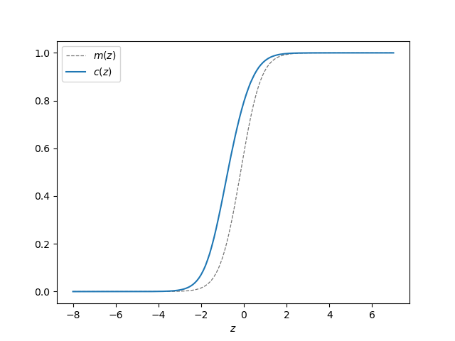
Figure 1. A numerical calculation of the boundary function $z\mapsto c(z)$ solving (3.1) and dominating the threshold $z\mapsto m(z)$ defined in Theorem 3.1.

The first main conclusion one can draw from Figure 1 is that, based on the configuration of model parameters defining the initial value $z=z(x,\pi):=\frac{\sigma^{2}}{2\alpha}\ln(\frac{\pi}{1-\pi})-\ln(x)$ of the process $Z$, introduced in Theorem 3.1, we may start our observations of the state space process $(Z,\Pi)$ from either one of three types of regions (e.g. for $z<-3.5$, $-3.5<z<2$, $z>2$ in Fig. 1).

In particular, the optimal timing problem for adopting an emissions reduction policy can experience the following three Phases:

• Immediate adoption. If $z$ is “relatively small” – that is, if the initial socioeconomic cost of pollution $x$ is relatively large with respect to the adjusted likelihood ratio $(\frac{\pi}{1-\pi})^{{\sigma^{2}}/({2\alpha})}$ – the initial belief $\pi$ of an increasing trend of future costs would be above $c(z)$, which would most likely require the optimal immediate adoption of the policy – unless we are absolutely certain of a decreasing future cost trend, i.e. $\pi\approx 0$.

• Dynamic decision making. If $z$ takes a “relatively intermediate” value, we are in a dynamic decision making phase, where we decide to adopt the policy – while learning the unknown future cost trend – when the stochastically-evolving learning process $\Pi^{\pi}_{\tau}$ exceeds the critical deterministically-evolving threshold $c(Z^{z}_{\tau})$ at some time $\tau\geq 0$.

• Never adopt. If $z$ is “relatively large” – that is, if the initial socioeconomic cost of pollution $x$ is relatively small compared to the adjusted likelihood ratio $(\frac{\pi}{1-\pi})^{{\sigma^{2}}/({2\alpha})}$ – or if we start from Phase (II) and $\Pi^{\pi}_{t}$ remains below the increasing (in time) threshold $c(Z^{z}_{t})$, we end up in this third phase, where we most likely never adopt the policy – unless we are absolutely certain of an increasing future cost trend, i.e. $\Pi_{\tau}\approx 1$ at some time $\tau\geq 0$.

In order to explore further the most interesting Phase (II) appearing in Figure 1, we can make two more observations: (a) While learning in Phase (II), i.e. as time passes and $Z_{\cdot}$ increases, implying that $c(Z_{\cdot})$ increases (see also properties of $c$ in Theorem 3.1), the decision maker requires a higher certainty about increasing future costs, in order to optimally adopt the policy; (b) The duration of time for which the observation process $(Z,\Pi)$ could stay in Phase (II), before adopting the policy or moving to Phase (III) and becoming “too late” for adopting the policy, is driven strongly by the value of the socioeconomic costs’ volatility $\sigma$, since it determines the speed of the time-coordinate process $Z$ (see Theorem 3.1).

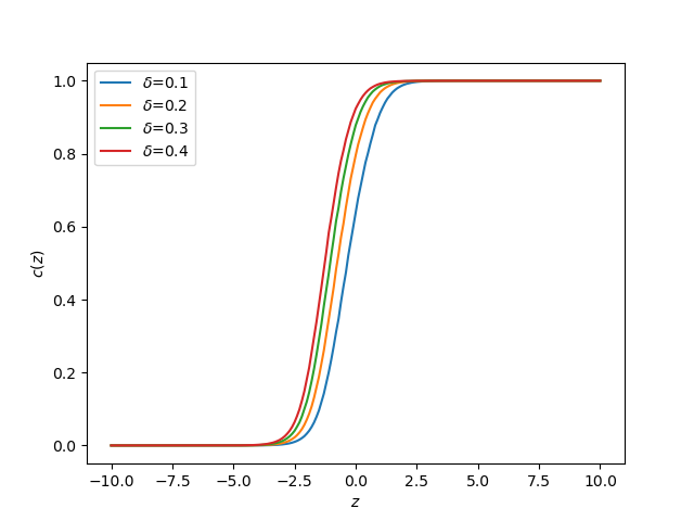
Figure 2. A numerical calculation of the boundary function $z\mapsto c(z)$ solving (3.1) with respect to different dissipation rates $\delta$ of the pollutant stock from the atmosphere.

Next, we aim at obtaining further results in terms of the sensitivity of the optimal policy adoption strategy with respect to several important model parameters.

We see from Figure 2 that the critical belief threshold $c(z)$ is increasing with higher dissipation rates $\delta$ of the pollutant stock from the atmosphere. That is, decision makers become more reluctant to adopt the policy if the pollutant emitted will dissipate at a faster rate, irrespective of their actions. Hence, they require their belief of an increasing future cost trend to reach a higher certainty level in order to be optimal to adopt an emission reduction policy. However, if the dissipation rate of pollutants is slow, then the importance of their actions increases, making the policy adoption optimal even for lower confidence levels about the future evolution of socioeconomic costs.

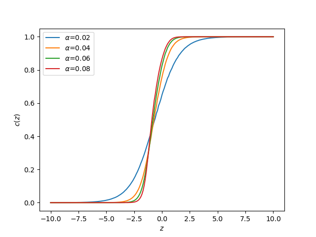
Figure 3. A numerical calculation of the boundary function $z\mapsto c(z)$ solving (3.1) with respect to different sizes $\alpha$ (resp. $-\alpha$) of the average rate of increase (resp. decrease) of future socioeconomic costs of pollution.

In Figure 3, we observe an interesting phenomenon. There is no clear monotonicity of the critical belief threshold $c(z)$ with respect to changes in the absolute value $\alpha$ of the average rate of increase/decrease of future socioeconomic costs of pollution. It seems though that, if we have more extreme alternative scenarios for the trend of future socioeconomic costs, i.e. higher $\alpha$-values, then the dynamic decision making phase (see Phase (II) above) shrinks in terms of time, and makes it more likely for the decision maker to end up in either an immediate policy adoption or never adopting the policy (both Phase (I) and Phase (III) extend). Essentially, this provides a quantitative way to capture the fact that, as the alternatives diverge from each other, the decision maker can learn sooner, i.e. after a relatively shorter time period $t$, whether it is optimal to adopt the policy or not. Contrary, when $\alpha$ decreases and the two alternatives come closer to each other, the dynamic decision making phase is extended. Hence, learning the unknown costs while examining whether a policy adoption would be optimal becomes increasingly more critical.

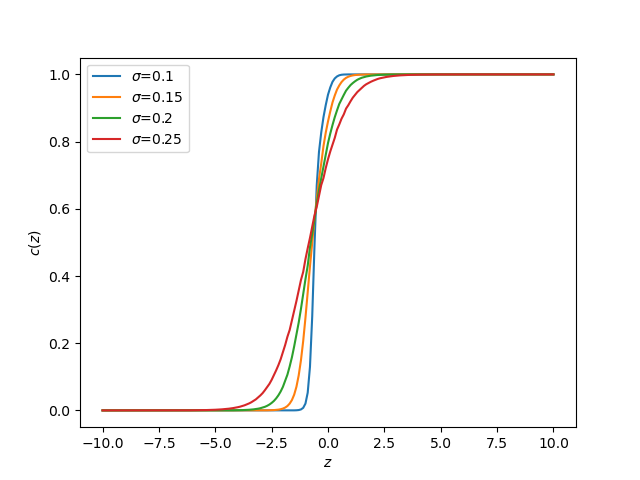
Figure 4. A numerical calculation of the boundary function $z\mapsto c(z)$ solving (3.1) with respect to different extends of volatility $\sigma$ in the socioeconomic costs of pollution.

We also observe in Figure 4 that the critical belief threshold $c(z)$ is clearly non-monotonic with respect to the volatility $\sigma$ of the socioeconomic costs of pollution. It seems that as the economic uncertainty around socioeconomic costs increases, i.e. higher $\sigma$-values, we get a larger dynamic decision making phase (see Phase (II) above). Therefore, learning the unknown costs becomes increasingly more critical in the decision making towards an optimal policy adoption. On the contrary, in times of low uncertainty the dynamic decision making phase shrinks in terms of time, and makes it more likely for the decision maker to end up in either an immediate policy adoption or never adopting the policy (both Phase (I) and Phase (III) extend). That is, with low volatility in socioeconomic costs, the future costs become less unpredictable and the current knowledge of decision makers would suffice to make an optimal decision to immediately or never adopt the policy. Interestingly, this phenomenon is contrary to the philosophy of the “value of waiting” (cf. [9] and [27], among others), where an increase in volatility usually results in less proactive decision makers, who are willing to postpone their actions in times of increased uncertainty.

4. On the proof of Theorem 3.1: Characterising the optimal emissions reduction time

In this section we develop a constructive proof of Theorem 3.1, leading to the characterisation of the optimal emissions reduction time. This will be distilled through a series of subsections and intermediate results.

4.1. Markovian formulation of Problem (2.7)

In order to solve the problem (2.7), and thus prove Theorem 3.1, we first observe that a Markovian reformulation is needed, since the unpredictable and non-observable nature of $\mu$ implies that $X$ is not a Markov process. The first step of our forthcoming analysis is thus to express the optimal stopping problem (2.7) in a Markovian framework.

The social planner’s information is modelled by the filtration $\mathcal{F}^{X}=(\mathcal{F}_{t}^{X})_{t\geq 0}$ generated by $X$ and augmented with $\mathbb{P}_{\pi}$-null sets, which is right-continuous (cf. [2, Theorem 2.35]). The social planner can then update their belief on the true value of $\mu$ according to new information as it gets revealed. In other words, by relying on filtering techniques (see, e.g. [26]), we can define the social planner’s Bayesian learning process $\Pi=(\Pi_{t})_{t\geq 0}$ on $(\Omega,\mathcal{F},\mathbb{P}_{\pi})$ as the ${\mathcal{F}}^{X}$-càdlàg martingale

(4.1) $$\Pi_{t}:=\mathbb{P}_{\pi}\big{(}\mu=\alpha\,\big{|}\,{\mathcal{F}}_{t}^{X}\big{)},\qquad\Pi_{0}=\pi\in(0,1).$$

Then, by [39, Section 4.2], the process $(X^{x},\Pi^{\pi})$ uniquely solves the SDE

(4.2) $$\begin{cases}dX_{t}^{x,\pi}=\left(\alpha\Pi_{t}^{\pi}-\alpha(1-\Pi_{t}^{\pi})\right)X_{t}^{x}dt+\sigma X_{t}^{x}d{W}_{t},&\quad X_{0}^{x,\pi}=x>0,\\ d\Pi_{t}^{\pi}=\frac{2\alpha}{{\sigma}}\Pi_{t}^{\pi}(1-\Pi_{t}^{\pi})d{W}_{t},&\quad\Pi_{0}^{\pi}=\pi\in(0,1),\end{cases}$$

where $W=(W_{t})_{t\geq 0}$ is the so-called innovation process, which is defined by

$$W_{t}:=\int_{0}^{t}\frac{\mu+\alpha-2\alpha\Pi^{\pi}_{s}}{\sigma}\,ds+B_{t},$$

and it is an ${\mathcal{F}}^{X}$-adapted Brownian motion under the probability measure $\mathbb{P}_{\pi}$. We note that the process $(X^{x,\pi},\Pi^{\pi})$ is also ${\mathcal{F}}^{{W}}$-adapted and, thus, we have ${\mathcal{F}}^{X}={\mathcal{F}}^{{W}}$. It is clear that $(X^{x,\pi},\Pi^{\pi})$ is now a Markov process under this new formulation.

Consider now a new probability space $(\widetilde{\Omega},\widetilde{\mathcal{F}},\widetilde{\mathbb{P}})$, on which we define a Brownian motion $\widetilde{W}$, adapted to its natural filtration ${\mathcal{F}}^{\widetilde{W}}$, augmented by $\widetilde{\mathbb{P}}$-null sets of $\widetilde{\mathcal{F}}$. On such a space, let $(\widetilde{X},\widetilde{\Pi})$ evolve as in (4.2), but with $W$ replaced by $\widetilde{W}$. Since (4.2) admits a unique strong solution, then

$$\text{Law}_{\mathbb{P}_{\pi}}(X,\Pi,\tau)=\text{Law}_{\widetilde{\mathbb{P}}}(\widetilde{X},\widetilde{\Pi},\widetilde{\tau}),$$

where $\widetilde{\tau}$ is an ${\mathcal{F}}^{\widetilde{W}}$-stopping time. Then, by means of the tower property in the expectation of (2.7), and using (4.1)–(4.2) and the aforementioned equality in law, the optimal stopping problem (2.7) becomes

(4.3) $$\inf_{\widetilde{\tau}\geq 0}\,\widetilde{\mathbb{E}}\Big{[}\int_{0}^{\widetilde{\tau}}e^{-rt}\widetilde{X}_{t}^{x,\pi}{P}_{t}^{p}dt+e^{-r\widetilde{\tau}}I+\int_{\widetilde{\tau}}^{\infty}e^{-rt}\widetilde{X}_{t}^{x,\pi}\widehat{P}_{t}^{p}dt\Big{]}.$$

From now on, with a slight abuse of notation, we shall write $(X,\Pi,\tau)$ as well as $(\Omega,\mathcal{F},\mathbb{P},\mathbb{E})$ instead of $(\widetilde{X},\widetilde{\Pi},\widetilde{\tau})$ and $(\widetilde{\Omega},\widetilde{\mathcal{F}},\widetilde{\mathbb{P}},\widetilde{\mathbb{E}})$, respectively.

Then, with regards to the Markovian nature of (4.3), given any initial values $(x,p,\pi)\in\mathbb{R}_{+}\times\mathbb{R}_{+}\times(0,1)$, we consider the optimal stopping problem

(4.4) $$V(x,p,\pi):=\inf_{\tau\geq 0}\,\mathbb{E}_{x,p,\pi}\Big{[}\int_{0}^{\tau}e^{-rt}{X}_{t}P_{t}dt+e^{-r\tau}I+\int_{\tau}^{\infty}e^{-rt}{X}_{t}\widehat{P}_{t}dt\Big{]},$$

where $\mathbb{E}_{x,p,\pi}[\,\cdot\,]:=\mathbb{E}[\,\cdot\,\big{|}\,X_{0}=x,P_{0}=p,\Pi_{0}=\pi]$ and the infimum is taken over all ${\mathcal{F}}^{X}$-stopping times $\tau$.

The next couple of Sections 4.1.1–4.1.2 concern some benchmark problems involving the two most extreme strategies of the social planner, i.e. never adopt or immediately adopt the environmental policy, which will be helpful in the dimensionality reduction of our problem in Section 4.1.3.

4.1.1. Never adopt the policy

Suppose that the social planner decides to postpone the policy forever, i.e. chooses $\tau=\infty$ in (4.4). Then, in view of (2.4), using the explicit expression (2.2) of $P^{p}$, invoking Fubini’s theorem, the total value $V_{\infty}$ of this strategy is

(4.5) $$\begin{split}V_{\infty}(x,p,\pi)&:=\mathbb{E}_{x,p,\pi}\left[\int_{0}^{\infty}e^{-rt}X_{t}P_{t}dt\right]\\ &=\mathbb{E}_{\pi}\left[\int_{0}^{\infty}e^{-rt}X_{t}^{x}\left(\frac{\beta E}{\delta}\left(1-e^{-\delta t}\right)+pe^{-\delta t}\right)dt\right]\\ &=\int_{0}^{\infty}e^{-rt}\,\mathbb{E}_{\pi}\left[X_{t}^{x}\right]\left(\frac{\beta E}{\delta}\left(1-e^{-\delta t}\right)+pe^{-\delta t}\right)dt\\ &=\int_{0}^{\infty}e^{-rt}x\left(\pi e^{\alpha t}+(1-\pi)e^{-\alpha t}\right)\left(\frac{\beta E}{\delta}\left(1-e^{-\delta t}\right)+pe^{-\delta t}\right)dt\\ &=\begin{cases}\beta Ex(\theta\pi+\rho)+xp(\theta_{0}\pi+\rho_{0}),&\text{if}\,\,r>\alpha,\\ +\infty&\text{if}\,\,r\leq\alpha,\end{cases}\end{split}$$

where $\mathbb{E}_{\pi}$ denotes the expectation conditioned on $\Pi_{0}=\pi$, and where we define, under the assumption that $r>\alpha$, the constants

(4.6) $$\begin{split}\theta&:=\frac{2\alpha(2r+\delta)}{(r-\alpha)(r+\alpha)(r+\delta-\alpha)(r+\delta+\alpha)}>0,\qquad\theta_{0}:=\frac{2\alpha}{(r+\delta-\alpha)(r+\delta+\alpha)}>0,\\ \rho&:=\frac{1}{(r+\delta+\alpha)(r+\alpha)}>0,\qquad\qquad\qquad\qquad\qquad\rho_{0}:=\frac{1}{r+\delta+\alpha}>0.\end{split}$$

4.1.2. Adopt the policy immediately

Suppose now that the social planner decides to adopt the policy immediately, i.e. chooses $\tau=0$ in (4.4). Then, in view of (2.4), using the explicit expression (2.6) of $\widehat{P}^{p}$ and invoking Fubini’s theorem, the resulting value $V_{0}$ is

(4.7) $$\begin{split}V_{0}(x,p,\pi):=I+\mathbb{E}_{x,p,\pi}\left[\int_{0}^{\infty}e^{-rt}X_{t}\widehat{P}_{t}dt\right]&=I+\int_{0}^{\infty}e^{-rt}x\left(\pi e^{\alpha t}+(1-\pi)e^{-\alpha t}\right)pe^{-\delta t}dt\\ &=\begin{cases}xp(\theta_{0}\pi+\rho_{0})+I,&\text{if}\,\,r+\delta>\alpha,\\ +\infty&\text{if}\,\,r+\delta\leq\alpha,\end{cases}\end{split}$$

for the previously defined positive constants $\theta_{0}$ and $\rho_{0}$ in (4.6).

4.1.3. Reformulation of Problem (4.4): Dimensionality reduction

Given that in environmental economics, especially in environmental policy adoption discussions, the aforementioned two strategies in Sections 4.1.1–4.1.2 are clearly plausible, we require that they are also admissible. Hence, we make the following assumption on the problem’s parameters, essentially ruling out the possibility of these strategies having value $+\infty$, i.e. yielding an infinite expected cost.

Assumption 4.1.

We assume that the discount rate $r$ and the highest average rate of environmental pollution costs $\alpha$ satisfy $r>\alpha$.

After rewriting the problem in the Markovian framework (4.4), it is obvious that the value function depends on all initial values $p,x>0$ and $\pi\in(0,1)$. Therefore, (4.4) seems to be a three-dimensional optimal stopping problem. However, thanks to the linearity of the running cost function, we will show that it reduces to a truly two-dimensional one, involving the process $(X^{x,\pi},\Pi^{\pi})$, while the deterministic evolution of the pollution stock $P^{p}$ will eventually affect the optimal timing of adopting the environmental policy only indirectly. A similar dimensionality reduction was conjectured in [37] for the full information case (from a two- to a one-dimensional problem); here we rigorously prove that such a reduction is possible, while extending it to our setting of the three-dimensional problem (4.4).

To see this, fix some initial values $(x,p,\pi)\in\mathbb{R}_{+}\times\mathbb{R}_{+}\times(0,1)$, and consider first the expectation

$$\mathbb{E}_{x,p,\pi}\left[\int_{0}^{\tau}e^{-rt}X_{t}P_{t}dt\right] =\mathbb{E}_{x,p,\pi}\left[\int_{0}^{\infty}e^{-rt}X_{t}P_{t}dt\right]-\mathbb{E}_{x,p,\pi}\left[\int_{\tau}^{\infty}e^{-rt}X_{t}P_{t}dt\right]$$

(4.8) $$=V_{\infty}(x,p,\pi)-\mathbb{E}_{x,p,\pi}\left[\int_{\tau}^{\infty}e^{-rt}X_{t}P_{t}dt\right],$$

where the latter equality follows from the definition (4.5) of $V_{\infty}$. By invoking the tower property, it follows again from (4.5) under Assumption 4.1 that

$$\mathbb{E}_{x,p,\pi}\left[\int_{\tau}^{\infty}e^{-rt}X_{t}P_{t}dt\right] =\mathbb{E}_{x,p,\pi}\left[e^{-r\tau}\left(\,\mathbb{E}_{x,p,\pi}\left[\int_{\tau}^{\infty}e^{-r(t-\tau)}X_{t}P_{t}dt\,\bigg{|}\,\mathcal{F}_{\tau}\right]\right)\right]$$

(4.9) $$=\mathbb{E}_{x,p,\pi}\Big{[}e^{-r\tau}V_{\infty}(X_{\tau},P_{\tau},\Pi_{\tau})\Big{]},$$

where the last equality is due to the strong Markov property of the process $(X,P,\Pi)$.

Using similar arguments as above, together with (4.7) under Assumption 4.1, we further obtain that

(4.10) $$\mathbb{E}_{x,p,\pi}\left[\int_{\tau}^{\infty}e^{-rt}X_{t}\widehat{P}_{t}dt\right]=\mathbb{E}_{x,p,\pi}\left[e^{-r\tau}\big{(}V_{0}(X_{\tau},\widehat{P}_{\tau},\Pi_{\tau})-I\big{)}\right].$$

Then, combining (4.1.3)–(4.10) and recalling from (2.5)–(2.6) that $\widehat{P}_{\tau}={P}_{\tau}$, we conclude that the value function (4.4) can be rewritten as

(4.11) $$\begin{split}V(x,p,\pi)&=\inf_{\tau\geq 0}\,\mathbb{E}_{x,p,\pi}\left[\int_{0}^{\tau}e^{-rt}X_{t}P_{t}dt+e^{-r\tau}I+\int_{\tau}^{\infty}e^{-rt}X_{t}\widehat{P}_{t}dt\right]\\ &=V_{\infty}(x,p,\pi)+\inf_{\tau\geq 0}\,\mathbb{E}_{x,\pi}\left[e^{-r\tau}\big{(}V_{0}(X_{\tau},{P}_{\tau},\Pi_{\tau})-V_{\infty}(X_{\tau},P_{\tau},\Pi_{\tau})\big{)}\right]\\ &=V_{\infty}(x,p,\pi)+\inf_{\tau\geq 0}\,\mathbb{E}_{x,\pi}\left[e^{-r\tau}\big{(}I-\beta E{X}_{\tau}(\theta\Pi_{\tau}+\rho)\big{)}\right]\\ &=V_{\infty}(x,p,\pi)-\sup_{\tau\geq 0}\,\mathbb{E}_{x,\pi}\left[e^{-r\tau}\big{(}\beta E{X}_{\tau}(\theta\Pi_{\tau}+\rho)-I\big{)}\right],\end{split}$$

where $\mathbb{E}_{x,\pi}[\,\cdot\,]:=\mathbb{E}[\,\cdot\,\big{|}\,X_{0}=x,\Pi_{0}=\pi]$.

Hence, the solution to the three-dimensional problem $V$ in (4.4) is given in terms of the solution to the two-dimensional optimal stopping problem with value function $U$ given by

(4.12) $$U(x,\pi) :=\sup_{\tau\geq 0}\,\mathbb{E}_{x,\pi}\left[e^{-r\tau}G(X_{\tau},\Pi_{\tau})\right],$$

where the supremum is taken over all ${\mathcal{F}}^{X}$-stopping times and the function

(4.13) $$G:\mathbb{R}_{+}\times(0,1)\mapsto\mathbb{R}\qquad\text{is defined by}\qquad G(x,\pi):=\beta Ex(\theta\pi+\rho)-I.$$

Therefore, the main aim in the remaining of this paper is to solve (4.12) and achieve the complete characterisation of the optimal strategy.

It is well known in optimal stopping theory that multi-dimensional optimal stopping problems cannot be solved in general via the standard guess-and-verify approach. On one hand, this solution method involves solving a partial differential equation (PDE) associated with the Hamilton-Jacobi-Bellman equation, but closed form solutions to PDEs can rarely be found. On the other hand, it is uncertain whether the usually (a priori) assumed smooth-fit condition of the value function (in two-dimensional stopping problems) holds along the free boundary function which defines the optimal stopping strategy. In the sequel, we employ a methodology to solve the problem consisting of a direct probabilistic approach and a transformation of the state-space.

Remark 4.2.

In contrast to the standard full information case [37], it will be shown in the forthcoming analysis that the optimal timing for the policy adoption is not given by a simple constant threshold strategy for the socioeconomic cost process $X$ any more. Instead, we will show in Section 4.2 that such a threshold will now be a function of the Bayesian learning process $\Pi$. What is even more interesting is that, in the process of completely characterising the optimal emissions reduction policy adoption, we will eventually express the optimal timing solely in terms of the learning process crossing a time- and model parameters-dependent boundary (see Sections 4.3–4.4 and Theorem 3.1).

4.2. Solution to the two-dimensional optimal stopping problem (4.12)

We are now ready to begin the analysis of Problem (4.12). To that end, by relying on optimal stopping theory [36], we firstly introduce the continuation region $\mathcal{C}$ and stopping region $\mathcal{S}$ defined by

(4.14) $$\begin{split}\mathcal{C}&:=\{(x,\pi)\in\mathbb{R}_{+}\times(0,1):\,U(x,\pi)>G(x,\pi)\},\\ \mathcal{S}&:=\{(x,\pi)\in\mathbb{R}_{+}\times(0,1):\,U(x,\pi)=G(x,\pi)\},\end{split}$$

as well as the stopping time

(4.15) $$\tau^{*}:=\inf\{t\geq 0:\,({X}^{x,\pi}_{t},\Pi^{\pi}_{t})\in\mathcal{S}\},$$

with the usual convention $\inf\emptyset=+\infty$. Later, we will show the optimality of $\tau^{*}$, as expected.

Before we proceed with addressing the problem, we notice that the boundary points $0$ and $1$ are entrance-not-exit for the diffusion $\Pi^{\pi}$, that is, $\Pi^{\pi}$ never atttains $0$ or $1$ in finite time whenever its initial value satisfies $\pi\in(0,1)$ (cf. [4, p.12]). The proof of the following result is omitted as it follows similar arguments to the one of [7, Lemma 3.1].

Lemma 4.3.

For all $\pi\in(0,1)$, we have

$$\mathbb{P}(\Pi_{t}^{\pi}\in(0,1)\,\,\forall\,\,t\geq 0)=1,$$

while, for $\pi\in\{0,1\}$, we have

$$\mathbb{P}(\Pi^{1}_{t}=1,\,\,\forall\,\,t\geq 0)=\mathbb{P}(\Pi^{0}_{t}=0,\,\,\forall\,\,t\geq 0)=1.$$

Also, we observe from (4.2) that

(4.16) $${X}_{t}^{x,\pi}=x\exp\left\{\int_{0}^{t}\Big{(}2\alpha\Pi_{s}^{\pi}-\alpha-\frac{\sigma^{2}}{2}\Big{)}ds+\sigma W_{t}\right\},\,\,\,\mathbb{P}_{x,\pi}\text{-a.s.}$$

In light of Assumption 4.1, we can prove that

$$\bigl{(}e^{-rt}{X}_{t}^{x,\pi}\bigr{)}_{t\geq 0}\quad\text{is a continuous super-martingale with last element}\quad\lim_{t\rightarrow\infty}e^{-rt}{X}_{t}^{x,\pi}=0.$$

This further implies, in view of $\Pi_{t}^{\pi}\in(0,1)$ for $\pi\in(0,1)$ due to Lemma 4.3, that we can adopt the convention

(4.17) $$e^{-r\tau}G({X}^{x,\pi}_{\tau},\Pi^{\pi}_{\tau})=0\qquad\text{on}\qquad\{\tau=\infty\}.$$

4.2.1. Well-posedness and initial properties of the value function $U$ defined in (4.12)

The next standard result ensures the well-posedness of the optimal stopping problem under study and its proof can be found in Appendix A.

Lemma 4.4.

The problem (4.12) is well-posed, the stopping time $\tau^{*}$ in (4.15) is optimal and

(4.18) $$\begin{cases}t\mapsto e^{-rt}U({X}^{x,\pi}_{t},\Pi_{t}^{\pi})&\text{is a supermartingale,}\\ t\mapsto e^{-r(t\wedge\tau^{*})}U({X}^{x,\pi}_{t\wedge\tau^{*}},\Pi^{\pi}_{t\wedge\tau^{*}})&\text{is a martingale.}\end{cases}$$

Next we obtain some further properties of the value function $U(x,\pi)$ and its proof can also be found in Appendix A.

Proposition 4.5.

Consider the value function $U$ in (4.12). Then, we have:

1. $U(\cdot,\cdot)$ is non-negative on $\mathbb{R}_{+}\times(0,1)$;

2. $x\mapsto U(x,\pi)$ is non-decreasing on $\mathbb{R}_{+}$;

3. $\pi\mapsto U(x,\pi)$ is non-decreasing on $(0,1)$;

4. $x\mapsto U(x,\pi)$ is Lipschitz continuous on $\mathbb{R}_{+}$;

5. $(x,\pi)\mapsto U(x,\pi)$ is continuous on $\mathbb{R}_{+}\times(0,1)$.

4.2.2. The structure of the state-space and the optimal strategy.

In this section, we aim at giving a rigorous geometric description of the continuation and stopping regions defined in (4.14). The following lemma is a direct consequence of the continuity of the value function of the optimal stopping problem (4.12) in Proposition 4.5.(v).

Lemma 4.6.

The continuation (resp., stopping) region $\mathcal{C}$ (resp., $\mathcal{S}$) defined in (4.14) is open (resp., closed).

The next proposition shows that the stopping region $\mathcal{S}$ is up-connected in both arguments $x$ and $\pi$; consequently the continuation region $\mathcal{C}$ is down-connected in both $x$ and $\pi$ (see Appendix A for the proof).

Proposition 4.7.

Let $(x_{0},\pi_{0})\in\mathbb{R}_{+}\times(0,1)$. The following properties hold:

1. $(x_{0},\pi_{0})\in\mathcal{S}\quad\Rightarrow\quad(x,\pi_{0})\in\mathcal{S}\quad\text{for all}\quad x\in[x_{0},\infty)$,

2. $(x_{0},\pi_{0})\in\mathcal{S}\quad\Rightarrow\quad(x_{0},\pi)\in\mathcal{S}\quad\text{for all}\quad\pi\in[\pi_{0},1)$.

In light of Proposition 4.7, we can define the boundary function $b:(0,1)\rightarrow\mathbb{R}_{+}$ by

(4.19) $$b(\pi):=\sup\{x>0:\,U(x,\pi)>G(x,\pi)\},\qquad\text{for all }\pi\in(0,1),$$

under the convention $\sup\emptyset=0$. Then, using Proposition 4.7.(i), we can obtain the shape of the continuation and stopping regions from (4.14) in the form

(4.20) $$\begin{split}\mathcal{C}=\{(x,\pi)\in\mathbb{R}_{+}\times(0,1)\,|\,x<b(\pi)\},\\ \mathcal{S}=\{(x,\pi)\in\mathbb{R}_{+}\times(0,1)\,|\,x\geq b(\pi)\},\end{split}$$

and the optimal stopping time from (4.15) takes the form of

(4.21) $$\tau^{*}:=\inf\{t\geq 0:\,{X}^{x,\pi}_{t}\geq b(\Pi^{\pi}_{t})\}.$$

Given all aforementioned results, we can also prove the following (see Appendix A).

Corollary 4.8.

The boundary function $b$ defined by (4.19) satisfies the properties:

1. $\pi\mapsto b(\pi)$ is non-increasing on $(0,1)$;

2. $\pi\mapsto b(\pi)$ is right-continuous on $(0,1)$.

4.3. A Parabolic Formulation of the two-dimensional optimal stopping problem (4.12)

In order to proceed further with our analysis and provide the complete characterisation of the optimal policy adoption timing, it is useful to make a transformation of the state-space. Notice that the process $({X},\Pi)$ defined in (4.2) is degenerate, in the sense that both components are driven by the same Brownian motion $W$. Therefore, we aim at maintaining the diffusive part in only one of the component processes, while transforming the other component to a completely deterministic bounded variation process, leading to a parabolic formulation. Similar transformations were employed in the literature [5, 6, 12, 17].

4.3.1. The transformed state-space process $(Z,\Pi)$.

We first define the process

(4.22) $${Z}_{t}^{z}:=\frac{\sigma^{2}}{2\alpha}\ln\Big{(}\frac{\Pi_{t}^{\pi}}{1-\Pi_{t}^{\pi}}\Big{)}-\ln({X}_{t}^{x,\pi}),\qquad Z_{0}=z:=\frac{\sigma^{2}}{2\alpha}\ln\Big{(}\frac{\pi}{1-\pi}\Big{)}-\ln(x),$$

which evolves deterministically (proof follows via Itô’s formula) according to

$$d{Z}_{t}=\frac{1}{2}\sigma^{2}dt,\quad Z_{0}=z,\qquad\text{or, equivalently}\qquad{Z}_{t}^{z}=z+\frac{1}{2}\sigma^{2}t,\quad t\geq 0.$$

Overall, the new state-space process $(Z,\Pi)$ is given by

(4.23) $$\begin{cases}dZ_{t}=\frac{1}{2}\sigma^{2}dt,&\quad Z_{0}=z:=\frac{\sigma^{2}}{2\alpha}\ln\big{(}\frac{\pi}{1-\pi}\big{)}-\ln(x)\in\mathbb{R},\\ d\Pi_{t}=\frac{2\alpha}{{\sigma}}\Pi_{t}(1-\Pi_{t})d{W}_{t},&\quad\Pi_{0}=\pi\in(0,1),\end{cases}$$

and its infinitesimal generator is defined for any $f\in C^{1,2}(\mathbb{R}\times(0,1))$ by

(4.24) $$(\mathcal{G}f)(z,\pi):=\frac{1}{2}\sigma^{2}\frac{\partial f}{\partial z}(z,\pi)+\frac{1}{2}\Big{(}\frac{2\alpha}{\sigma}\Big{)}^{2}\pi^{2}(1-\pi)^{2}\frac{\partial^{2}f}{\partial\pi^{2}}(z,\pi).$$

4.3.2. The transformed value function $W(z,\pi)$.

For any $(x,\pi)\in\mathbb{R}_{+}\times(0,1)$, define the transformation

(4.25) $$T:=(T_{1},T_{2}):\mathbb{R}_{+}\times(0,1)\to\mathbb{R}\times(0,1),\qquad(T_{1}(x,\pi),T_{2}(x,\pi))=\Big{(}\frac{\sigma^{2}}{2\alpha}\ln\Big{(}\frac{\pi}{1-\pi}\Big{)}-\ln(x),\pi\Big{)},$$

which is invertible and its inverse is given by

(4.26) $$T^{-1}(z,\pi)=\Big{(}e^{-z}\Big{(}\frac{\pi}{1-\pi}\Big{)}^{\frac{\sigma^{2}}{2\alpha}},\pi\Big{)},\quad(z,\pi)\in\mathbb{R}\times(0,1).$$

Using the latter inverse transformation, we firstly introduce the transformed version $W(z,\pi)$ of the value function $U(x,\pi)$ defined in (4.12) by

(4.27) $$W(z,\pi) :=U\Big{(}e^{-z}\Big{(}\frac{\pi}{1-\pi}\Big{)}^{\frac{\sigma^{2}}{2\alpha}},\pi\Big{)},$$

and secondly express the process $X$ as a function of the new state-space process $(Z,\Pi)$; namely,

(4.28) $${X}_{t}^{x,\pi}=e^{-{Z}_{t}^{z}}\Big{(}\frac{\Pi_{t}^{\pi}}{1-\Pi_{t}^{\pi}}\Big{)}^{\frac{\sigma^{2}}{2\alpha}},\qquad t\geq 0.$$

In view of these, the optimal stopping problem (4.12) can be rewritten in terms of the process $(Z,\Pi)$ defined in (4.23) as

(4.29) $$W(z,\pi) =\sup_{\tau\geq 0}\,\mathbb{E}_{z,\pi}\left[e^{-r\tau}F(Z_{\tau},\Pi_{\tau})\right],\qquad\text{where}\quad F(z,\pi):=\beta Ee^{-z}\Big{(}\frac{\pi}{1-\pi}\Big{)}^{\frac{\sigma^{2}}{2\alpha}}(\theta\pi+\rho)-I,$$

and $\mathbb{E}_{z,\pi}$ denotes the expectation under $\mathbb{P}$, conditional on $Z_{0}=z$ and $\Pi_{0}=\pi$.

In view of the relationship (4.27), the value function $W(\cdot,\cdot)$ inherits important properties which have already been proved for $U(\cdot,\cdot)$ in Section 4.2. In particular, we have directly from Proposition 4.5.(v) the following result.

Proposition 4.9.

The transformed value function $(z,\pi)\mapsto W(z,\pi)$ is continuous on $\mathbb{R}\times(0,1)$.

Similarly to Section 4.2, we can also define the corresponding continuation and stopping regions by

(4.30) $$\begin{split}\mathcal{C}^{\prime}&:=\{(z,\pi)\in\mathbb{R}\times(0,1)\,|\,W(z,\pi)>F(z,\pi)\},\\ \mathcal{S}^{\prime}&:=\{(z,\pi)\in\mathbb{R}\times(0,1)\,|\,W(z,\pi)=F(z,\pi)\}.\end{split}$$

Given Proposition 4.9, the continuation region $\mathcal{C}^{\prime}$ is open and the stopping region $\mathcal{S}^{\prime}$ is closed and given that $T$ from (4.25) is a global diffeomorphism, we actually have

$${\mathcal{C}^{\prime}}=T({\mathcal{C}})\quad\text{and}\quad{\mathcal{S}^{\prime}}=T({\mathcal{S}}),$$

where $\mathcal{C}$ and $\mathcal{S}$ are the continuation and stopping regions from (4.14) under $(x,\pi)$-coordinates. Hence, the corresponding optimal stopping time $\tau^{*}$ from (4.15) becomes

(4.31) $$\tau^{*}:=\inf\{t\geq 0\,|\,(Z^{z}_{t},\Pi^{\pi}_{t})\in\mathcal{S}^{\prime}\}.$$

4.3.3. The transformed optimal stopping boundary.

In order to obtain the explicit structure of the regions ${\mathcal{C}^{\prime}}$ and $\mathcal{S}^{\prime}$ from (4.30), we recall the inverse transformation $T^{-1}$ in (4.26), the expression of $\mathcal{C}$ in (4.20) and the positivity of $b$, to obtain

$$(z,\pi)\in{\mathcal{C}^{\prime}} \Leftrightarrow \Big{(}e^{-z}\Big{(}\frac{\pi}{1-\pi}\Big{)}^{\frac{\sigma^{2}}{2\alpha}},\pi\Big{)}\in{\mathcal{C}}\quad\Leftrightarrow\quad e^{-z}\Big{(}\frac{\pi}{1-\pi}\Big{)}^{\frac{\sigma^{2}}{2\alpha}}<b(\pi)\quad\Leftrightarrow\quad z>\ln\bigg{(}\frac{1}{b(\pi)}\Big{(}\frac{\pi}{1-\pi}\Big{)}^{\frac{\sigma^{2}}{2\alpha}}\bigg{)}.$$

Then, by defining

(4.32) $$c^{-1}(\pi):=\ln\bigg{(}\frac{1}{b(\pi)}\Big{(}\frac{\pi}{1-\pi}\Big{)}^{\frac{\sigma^{2}}{2\alpha}}\bigg{)}=\ln\bigg{(}\Big{(}\frac{\pi}{1-\pi}\Big{)}^{\frac{\sigma^{2}}{2\alpha}}\bigg{)}-\ln\big{(}b(\pi)\big{)},$$

we can obtain the structure of the continuation and stopping regions of $W$, which take the form

(4.33) $$\begin{split}\mathcal{C}^{\prime}&:=\{(z,\pi)\in\mathbb{R}\times(0,1)\,|\,z>c^{-1}(\pi)\},\\ \mathcal{S}^{\prime}&:=\{(z,\pi)\in\mathbb{R}\times(0,1)\,|\,z\leq c^{-1}(\pi)\}.\end{split}$$

By using the expression (4.32) of the function $c^{-1}(\cdot)$ and taking into account the fact that $b(\cdot)$ is non-increasing due to Corollary 4.8.(i), we obtain for any $\varepsilon>0$, that

$$c^{-1}(\pi+\varepsilon)-c^{-1}(\pi)=\int_{\pi}^{\pi+\varepsilon}\frac{\sigma^{2}}{2\alpha u(1-u)}du-\big{(}\ln b(\pi+\varepsilon)-\ln b(\pi)\big{)}\geq\int_{\pi}^{\pi+\varepsilon}\frac{\sigma^{2}}{2\alpha u(1-u)}du>0.$$

That is, $c^{-1}(\cdot)$ is strictly increasing. Moreover, the definition (4.32) of $c^{-1}(\cdot)$ and the right-continuity of $b(\cdot)$ on $(0,1)$ due to Corollary 4.8.(i), imply that $c^{-1}(\cdot)$ is right-continuous. These properties are summarised below.

Lemma 4.10.

The function $c^{-1}(\cdot)$ defined in (4.34) is strictly increasing and right-continuous on $(0,1)$.

In light of Lemma 4.10, we may now define the function

(4.34) $$c(z):=\inf\{\pi\in(0,1)\,|\,z\leq c^{-1}(\pi)\}.$$

In the following result, we prove some properties of $z\mapsto c(z)$ and that it identifies with the optimal stopping boundary of Problem (4.29). The proof can be found in Appendix A.

Proposition 4.11.

The free boundary $c$ defined in (4.34) satisfies the following properties:

1. $c(\cdot)$ is non-decreasing on $\mathbb{R}$;

2. We have $0\leq c(z)\leq 1$ for all $z\in\mathbb{R}$ with $\lim_{z\downarrow-\infty}c(z)=0$ and $\lim_{z\uparrow\infty}c(z)=1$;

3. $c(\cdot)$ is continuous on $\mathbb{R}$.

4. The structure of the continuation and stopping regions for (4.29) take the form

   (4.35) $$\begin{split}\mathcal{C}^{\prime}&:=\{(z,\pi)\in\mathbb{R}\times(0,1)\,|\,\pi<c(z)\},\\ \mathcal{S}^{\prime}&:=\{(z,\pi)\in\mathbb{R}\times(0,1)\,|\,\pi\geq c(z)\}.\end{split}$$

4.4. Smooth-fit property and integral equation for the transformed stopping boundary

We firstly define (using Dynkin’s formula and standard localisation arguments) the distance of the transformed value function $W$ from its intrinsic value $F$ by

(4.36) $$w(z,\pi) :=W(z,\pi)-F(z,\pi)=\sup_{\tau\geq 0}\,\mathbb{E}_{z,\pi}\bigg{[}\int_{0}^{\tau}e^{-rt}q(Z_{t},\Pi_{t})dt\bigg{]},$$

where the function $q(\cdot,\cdot)$ is defined by

(4.37) $$q(z,\pi):=\beta Ee^{-z}\Bigl{(}\frac{\pi}{1-\pi}\Bigr{)}^{\frac{\sigma^{2}}{2\alpha}}\Big{(}\big{(}(\alpha-r)\theta+2\alpha\rho\big{)}\pi-(\alpha+r)\rho\Big{)}+rI\qquad\text{for all }(z,\pi)\in\mathbb{R}\times(0,1).$$

In the following result, we provide properties of $w$ (see Appendix A for their proofs) that will be later used in order to derive its smooth-fit property.

Proposition 4.12.

The function $w$ defined by (4.36) satisfies the following properties:

1. $z\mapsto w(z,\pi)$ is non-decreasing on $\mathbb{R}$;

2. $\pi\mapsto w(z,\pi)$ is non-increasing on $(0,1)$.

3. $w\in C^{1,2}(\mathcal{C}^{\prime})$ and uniquely solves on any open set $\mathcal{R}$, whose closure is a subset of $\mathcal{C}^{\prime}$, the PDE

   (4.38) $$(\mathcal{G}-r)m(z,\pi)=-q(z,\pi),\quad\text{for}\quad(z,\pi)\in\mathcal{R},\qquad\text{with}\quad\left.m\right|_{\partial\mathcal{R}}=\left.w\right|_{\partial\mathcal{R}}.$$

Since the transformed boundary function $c(\cdot)$ is non-decreasing on $\mathbb{R}$ due to Proposition 4.11.(i), we observe that the process $(Z^{z},\Pi^{\pi})$ does not necessarily enter immediately into the stopping region $\mathcal{S}^{\prime}$ expressed by (4.35), when started from a point $(z,\pi)\in\partial\mathcal{C}$. Hence, a classical proof of the continuity of $\pi\mapsto\frac{\partial w}{\partial\pi}(z,\pi)$, for all $z\in\mathbb{R}$, (see [36] for examples) is not feasible. In order to prove the latter result we follow arguments as those in the proof of [6, Lemma 5.5]; see Appendix A for the detailed technical proof.

Proposition 4.13.

Consider the function $w$ defined by (4.36). For each $z\in\mathbb{R}$, we have that $\pi\mapsto\frac{\partial w}{\partial\pi}(z,\pi)$ is continuous on $(0,1)$.

In the sequel, we employ the continuity of $c$ from Proposition 4.11.(iii), the regularity and monotonicity of $w$ from Proposition 4.12, the smooth-fit property from Proposition 4.13 and the fact that the component process $(Z_{t})_{t\geq 0}$ is actually a time-variable, to use the local-time-space formula from [33, Theorem 3.1, Remark 3.2.(2)] on $(e^{-rt}w(Z_{t},\Pi_{t}))_{t\geq 0}$ and obtain the following result. This technical proof can also be found in Appendix A.

Theorem 4.14.

For any $(z,\pi)\in\mathbb{R}\times(0,1)$, the function $w$ defined in (4.36) can be represented by

$$w(z,\pi)=\mathbb{E}_{z,\pi}\bigg{[}\int_{0}^{\infty}e^{-rt}q(Z_{t},\Pi_{t}){\bf 1}_{\{\Pi_{t}\leq c(Z_{t})\}}dt\bigg{]}=\int_{0}^{\infty}e^{-rt}\left(\int_{0}^{c(z+\frac{1}{2}\sigma^{2}t)}q\big{(}z+\tfrac{1}{2}\sigma^{2}t,\pi^{\prime}\big{)}p_{t}(\pi,\pi^{\prime})d\pi^{\prime}\right)dt,$$

where $p_{t}(\pi,\pi^{\prime})=\frac{d\mathbb{P}_{\pi}(\Pi^{\pi}_{t}\leq\pi^{\prime})}{d\pi^{\prime}}$ denotes the transition density of $(\Pi^{\pi}_{t})_{t\geq 0}$.

In light of the above integral representation of $w$, we are now finally ready to completely characterise the boundary function $c$, and therefore complete the proof of our main Theorem 3.1. To that end, we define, for each $z\in\mathbb{R}$,

(4.39) $$m(z):=\inf\{\pi\in(0,1)\,|\,q(z,\pi)<0\},$$

which uniquely exists since $q(z,0+)=rI>0$, $q(z,1-)=-\infty$ and $\pi\mapsto q(z,\pi)$ is continuous and decreasing.

By evaluating the integral representation of $w$ in Theorem 4.14 at $\pi=c(z)$ for each $z\in\mathbb{R}$ and using the fact that $w(z,c(z))=0$, we obtain that $c$ solves the integral equation (cf. (3.1))

$$0=\int_{0}^{\infty}e^{-rt}\left(\int_{0}^{c(z+\frac{1}{2}\sigma^{2}t)}q\big{(}z+\tfrac{1}{2}\sigma^{2}t,\pi^{\prime}\big{)}p_{t}(c(z),\pi^{\prime})d\pi^{\prime}\right)dt.$$

Moreover, by letting

$$\mathcal{M}:=\{f:\mathbb{R}\mapsto\mathbb{R}\,|\,\text{f is non-decreasing, continuous and satisfies $f(z)\geq m(z)$ for all $z\in\mathbb{R}$}\},$$

the four-step procedure (without additional challenges) developed in [34] via the exploitation of the superharmonic property of $W$, can be employed to conclude that the boundary function $c$ defined by (4.34) is the unique solution in $\mathcal{M}$.

Upon collecting all the results developed in this section, the constructive proof of Theorem 3.1 is therefore complete.

5. Conclusions

This paper focuses on the social planner’s option to adopt an environmental policy implying a once-and-for-all reduction in the current emissions. In the course of this, we allow for two layers of uncertainty about the future social and economic consequences of the environmental damage, by letting the associated process $X$ fluctuate stochastically and allowing the decision maker to have only partial information about the trend of $X$. Introducing partial information about key parameters in the stochastic dynamics of socioeconomic costs of pollution reflects better the current real-life debate on the actions required to contrast climate change. The rigorous and complete treatment of this nontrivial novel problem represents the main contribution of our work. We suitably tackle this increased uncertainty on the after-effects of pollution and show that it plays a considerably important role in the optimal timing of policy adoption. A first important effect of additional uncertainty is indeed that the optimal policy adoption is no longer triggered by constant thresholds, as in the full information case [37].

As a matter of fact, without relying on the traditional guess-and-verify-approach (non-feasible in our multi-dimensional case), we show via probabilistic means and state-space transformation techniques that it is optimal to abate emissions when the stochastic socioeconomic costs $X$ hits or exceeds an upper tolerance level $b(\Pi)$, depending on the filtering estimate process $\Pi$ of the unknown drift of $X$. Such a stopping rule can be equivalently expressed in terms of a boundary $c$, depending on a scaled time coordinate $Z$: It is optimal to reduce the stock of pollutants when the belief process $\Pi$ – likelihood of having on average increasing socioeconomic costs – becomes “decisive enough” and exceeds the time-dependent percentage $c(Z)$. Sensitivity of the optimal policy adoption with respect to the model’s parameters is studied by solving numerically the nonlinear integral equation which is uniquely solved by the boundary $c$.

Our work provides a first tractable example of a stylised model aiming at describing the role of different sources of uncertainty in the typically irreversible social decisions related to climate policy. Clearly, there are various direction towards our analysis can be generalised. First of all, it would be interesting to account for Knightian uncertainty in the dynamics of the cost process (see, e.g., [13], [29], [42] for examples of real-options/irreversible investment problems under Knightian uncertainty). This would in turn allow to comparatively study how the different specifications of uncertainty (no uncertainty, Bayesian uncertainty, Knightian uncertainty) affect the optimal emissions reduction policy. Second of all, it would be important to allow for the transboundary effect of pollution and thus incorporate strategic interaction between different decision makers. How the free-riding effect will depend on the specification of uncertainty would represent a key question in that context (see [21], [22] for recent works on public good contribution games under uncertainty).

Appendix A Technical Proofs

Proof of Lemma 4.4. We show below that the process $({X}_{t},\Pi_{t})$ from (4.2) satisfies the condition

(A.1) $$\mathbb{E}_{x,\pi}\left[\sup_{t\geq 0}e^{-rt}G({X}_{t},\Pi_{t})\right]<+\infty,$$

which will then imply, according to [18, Theorem D.12], that the stopping time (4.15) is optimal for the well-posed problem (4.12), as well as ensures that (4.18) holds true.

To that end, notice that using the expression of $G$ in (4.13), we obtain

$$\mathbb{E}_{x,\pi}\left[\sup_{t\geq 0}e^{-rt}\big{(}\beta E{X}_{t}(\theta\Pi_{t}+\rho)-I\big{)}\right] \leq\mathbb{E}_{x,\pi}\left[\sup_{t\geq 0}e^{-rt}\big{(}\beta E{X}_{t}(\theta\Pi_{t}+\rho)\big{)}\right]$$

$$\leq\mathbb{E}_{x,\pi}\left[\sup_{t\geq 0}e^{-rt}\beta E(\theta+\rho){X}_{t}\right],$$

where the latter inequality is due to the positivity of $e^{-rt}\beta E\theta{X}_{t}$ and the property $\Pi_{t}^{\pi}\in(0,1)$ for $\pi\in(0,1)$ (Cf. Lemma 4.3). Thus, using the explicit expression of $X$ in (4.16), the upper bound becomes

$$\mathbb{E}\left[\sup_{t\geq 0}e^{-rt}\beta E(\theta+\rho){X}_{t}^{x,\pi}\right] =\beta E(\theta+\rho)x\,\mathbb{E}\left[\sup_{t\geq 0}e^{-rt}\,e^{\int_{0}^{t}(2\alpha\Pi_{s}^{\pi}-\alpha-\frac{\sigma^{2}}{2})ds+\sigma W_{t}}\right]$$

$$\leq\beta E(\theta+\rho)x\,\mathbb{E}\left[\sup_{t\geq 0}e^{-bt+\sigma W_{t}}\right],$$

where we define the constant $b:=r-\alpha+\frac{\sigma^{2}}{2}>0$. Hence, using [19, Section 3.5.C], which implies that

$$\text{for $z>0$,}\qquad\mathbb{P}\Bigl{(}\sup_{t\geq 0}\big{\{}-bt+{\sigma}W_{t}\big{\}}\in dz\Bigr{)}=\tfrac{2b}{{\sigma}^{2}}e^{-\frac{2b}{{\sigma}^{2}}z}dz,$$

we can conclude that

$$\mathbb{E}\left[\sup_{t\geq 0}e^{-bt+{\sigma}W_{t}}\right]=\frac{2b}{{\sigma}^{2}}\int_{0}^{\infty}e^{z}e^{-\frac{2b}{{\sigma}^{2}}z}dz=\frac{2b}{{\sigma}^{2}}\int_{0}^{\infty}e^{-\big{(}\frac{2b}{{\sigma}^{2}}-1\big{)}}dz<+\infty,$$

where we used the fact that ${2b}>{{\sigma}^{2}}$ due to Assumption 4.1. Hence, we conclude that (A.1) holds. $\quad\Box$

Proof of Proposition 4.5. Proof of part (i). This is a trivial consequence of the definition (4.12) and the property (4.17), which imply the non-negativity of $U(x,\pi)$, since never stopping, i.e. choosing $\tau=\infty$, is an admissible strategy which results in a payoff of zero.

Proof of part (ii). By the definition (4.12) of $U$, the explicit expression (4.16) of ${X}^{x,\pi}$ which implies that $x\mapsto{X}^{x,\pi}_{\tau}$ is increasing for any stopping time $\tau$, and the definition (4.13) of $G$ which implies that $x\mapsto G(x,\pi)$ is increasing for any $\pi\in(0,1)$, we conclude that $x\mapsto U(x,\pi)$ is increasing as well.

Proof of part (iii). Using the above properties together with the fact that $\pi\mapsto\Pi^{\pi}_{\tau}$ is increasing for any stopping time $\tau$ (see the comparison theorem of Yamada and Watanabe, e.g. [19, Proposition 2.18]), the explicit expression (4.16) of ${X}^{x,\pi}$ which then implies that $\pi\mapsto{X}^{x,\pi}_{\tau}$ is also increasing for any stopping time $\tau$, and the definition (4.13) of $G$ which implies that $\pi\mapsto G(x,\pi)$ is increasing for any $\pi\in(0,1)$, we conclude by the definition (4.12) of $U$ that $\pi\mapsto U(x,\pi)$ is increasing as well.

Proof of part (iv). For any $0<x_{1}<x_{2}$ and $\pi\in(0,1)$, we define by $\tau^{*}:=\tau^{*}(x_{2},\pi)$ the optimal stopping time for the value function $U(x_{2},\pi)$ in (4.12). Then using the monotonicity of $U(\cdot,\pi)$ from part (ii) and the expression (4.12) of $U$, we obtain for a sufficiently large constant $C_{1}(x,\pi_{2})$ (cf. Lemma 4.4)

$$0 \leq U(x_{2},\pi)-U(x_{1},\pi)$$

$$\leq\mathbb{E}_{x_{2},\pi}\left[e^{-r\tau^{*}}\big{(}\beta E{X}_{\tau^{*}}(\theta\Pi_{\tau^{*}}+\rho)-I\big{)}\right]-\mathbb{E}_{x_{1},\pi}\left[e^{-r\tau^{*}}\big{(}\beta E{X}_{\tau^{*}}(\theta\Pi_{\tau^{*}}+\rho)-I\big{)}\right]$$

$$=(x_{2}-x_{1})\,\mathbb{E}\left[e^{-r\tau^{*}}\beta E{X}^{1,\pi}_{\tau^{*}}(\theta\Pi^{\pi}_{\tau^{*}}+\rho)\right]$$

(A.2) $$\leq(x_{2}-x_{1})\,\mathbb{E}\left[e^{-r\tau^{*}}\beta E{X}^{1,1}_{\tau^{*}}(\theta+\rho)\right]\leq C_{1}(x,\pi_{2})(x_{2}-x_{1}),$$

where the penultimate inequality follows from the positivity of coefficients, $\Pi_{t}\in(0,1)$ for all $t\geq 0$ due to Lemma 4.3, and ${X}^{1,\pi}_{\tau^{*}}\leq{X}^{1,1}_{\tau^{*}}$, since $\pi\mapsto{X}^{x,\pi}_{\tau^{*}}$ is increasing for the fixed $\tau^{*}$.

Proof of part (v). To show this, it is sufficient to use part (iv) and additionally prove that

$$\pi\mapsto U(x,\pi)\quad\text{is continuous.}$$

To that end, fix $x>0$, $0<\pi_{1}<\pi_{2}<1$ and define by $\overline{\tau}^{*}:=\tau^{*}(x,\pi_{2})$ the optimal stopping time for $U(x,\pi_{2})$ in (4.12). Using the monotonicity of $U(x,\cdot)$ from part (iii) and the expression in (4.12), we deduce that

$$0 \leq U(x,\pi_{2})-U(x,\pi_{1})$$

$$\leq\mathbb{E}_{x,\pi_{2}}\left[e^{-r\overline{\tau}^{*}}\big{(}\beta E{X}_{\overline{\tau}^{*}}(\theta\Pi_{\overline{\tau}^{*}}+\rho)-I\big{)}\right]-\mathbb{E}_{x,\pi_{1}}\left[e^{-r\overline{\tau}^{*}}\big{(}\beta E{X}_{\overline{\tau}^{*}}(\theta\Pi_{\overline{\tau}^{*}}+\rho)-I\big{)}\right]$$

(A.3) $$=\mathbb{E}\left[e^{-r\overline{\tau}^{*}}\beta E\big{(}{X}^{x,\pi_{2}}_{\overline{\tau}^{*}}(\theta\Pi^{\pi_{2}}_{\overline{\tau}^{*}}+\rho)-{X}^{x,\pi_{1}}_{\overline{\tau}^{*}}(\theta\Pi^{\pi_{1}}_{\overline{\tau}^{*}}+\rho)\big{)}\right].$$

We now aim at taking limits as $\pi_{1}\to\pi_{2}$. To that end, we notice that, due to the positivity of coefficients, $\Pi_{t}\in(0,1)$ for all $t\geq 0$ thanks to Lemma 4.3, and ${X}^{x,0}_{\overline{\tau}^{*}}\leq{X}^{x,\pi_{1}}_{\overline{\tau}^{*}}\leq{X}^{x,\pi_{2}}_{\overline{\tau}^{*}}\leq{X}^{x,1}_{\overline{\tau}^{*}}$ (since $\pi\mapsto{X}^{x,\pi}_{\overline{\tau}^{*}}$ is increasing for the fixed $\overline{\tau}^{*}$), we conclude that

$$e^{-r\overline{\tau}^{*}}\beta E\big{(}{X}^{x,\pi_{2}}_{\overline{\tau}^{*}}(\theta\Pi^{\pi_{2}}_{\overline{\tau}^{*}}+\rho)-{X}^{x,\pi_{1}}_{\overline{\tau}^{*}}(\theta\Pi^{\pi_{1}}_{\overline{\tau}^{*}}+\rho)\big{)}\leq e^{-r\overline{\tau}^{*}}\beta E\big{(}{X}^{x,1}_{\overline{\tau}^{*}}(\theta+\rho)-{X}^{x,0}_{\overline{\tau}^{*}}\rho\big{)},$$

such that

$$\mathbb{E}\left[e^{-r\overline{\tau}^{*}}\beta E\big{(}{X}^{x,\pi_{2}}_{\overline{\tau}^{*}}(\theta\Pi^{\pi_{2}}_{\overline{\tau}^{*}}+\rho)-{X}^{x,\pi_{1}}_{\overline{\tau}^{*}}(\theta\Pi^{\pi_{1}}_{\overline{\tau}^{*}}+\rho)\big{)}\right]\leq x\,C_{2}(x,\pi_{2}).$$

Here, $C_{2}(x,\pi_{2})>0$ is a sufficiently large constant (note that the calculations in the proof of Lemma 4.4 imply the finiteness of the expectation). It thus follows that the dominated convergence theorem can be applied when letting $\pi_{1}\to\pi_{2}$ in (A.3), so that that the upper bound in (A.3) tends to zero. This implies the continuity of $\pi\mapsto U(x,\pi)$ and completes the proof. $\quad\Box$

Proof of Proposition 4.7. In order to prove these results, we firstly define the distance $u$ of the value function from its intrinsic value, whose expression is obtained by an application of Dynkin’s formula:

$$\begin{split}u(x,\pi)&:=U(x,\pi)-G(x,\pi)=\sup_{\tau\geq 0}\,\mathbb{E}_{x,\pi}\left[\int_{0}^{\tau}e^{-rt}\Big{(}\beta E\bigl{(}\theta(\alpha-r)+2\alpha\rho\bigr{)}{X}_{t}\Pi_{t}-(\alpha+r)\beta E\rho{X}_{t}+rI\Big{)}dt\right].\end{split}$$

Proof of part (i). Thanks to Assumption 4.1, we can easily verify that $\theta(\alpha-r)+2\alpha\rho<0$. Then, from the explicit solution of ${X}^{x,\pi}$ given in (4.16), it is clear that $x\mapsto{X}^{x,\pi}$ is increasing. This implies that for any stopping time $\tau$, we have for any $\pi\in(0,1)$, that

$$x\mapsto\mathbb{E}_{x,\pi}\left[\int_{0}^{\tau}e^{-rt}\left(\beta E\bigl{(}\theta(\alpha-r)+2\alpha\rho\bigr{)}{X}_{t}\Pi_{t}-(\alpha+r)\beta E\rho{X}_{t}+rI\right)dt\right]\quad\text{is decreasing on }\mathbb{R},$$

which implies that $x\mapsto u(x,\pi)$ is also decreasing.

Suppose now that $(x_{0},\pi_{0})\in\mathcal{S}$ and consider $(x,\pi_{0})$ for some $x\geq x_{0}$. By the monotonicity of $u(\cdot,\pi)$, we have $u(x,\pi_{0})\leq u(x_{0},\pi_{0})=0.$ Since $u(x,\pi_{0})$ is non-negative by definition, we must have $u(x,\pi_{0})=0$, thus $U(x,\pi)=G(x,\pi)$, i.e. $(x,\pi_{0})\in\mathcal{S}$.

Proof of part (ii). Recall that $\pi\mapsto\Pi^{\pi}$ is increasing by the comparison theorem of Yamada and Watanabe (see, e.g., [19, Proposition 2.18]) and consequently that $\pi\mapsto{X}^{x,\pi}$ is also increasing in light of (4.16). Therefore, for any stopping time $\tau$, we clearly have for any $x>0$, that

$$\pi\mapsto\mathbb{E}_{x,\pi}\left[\int_{0}^{\tau}e^{-rt}\left(\beta E\bigl{(}\theta(\alpha-r)+2\alpha\rho\bigr{)}{X}_{t}\Pi_{t}-(\alpha+r)\beta E\rho{X}_{t}+rI\right)dt\right]\quad\text{is decreasing on }(0,1),$$

implying that $\pi\mapsto u(x,\pi)$ is also decreasing.

This in turn implies that for $(x_{0},\pi_{0})\in\mathcal{S}$ and $(x_{0},\pi)$ for some $\pi\geq\pi_{0}$, we have $u(x_{0},\pi)\leq u(x_{0},\pi_{0})=0$. We then conclude that $u(x_{0},\pi)=0$, i.e. $(x_{0},\pi)\in\mathcal{S}$, which completes the proof. $\quad\Box$

Proof of Corollary 4.8. Proof of part (i). This follows directly from the definition (4.19) of $b$, the shape of continuation and stopping regions in (4.20) and Proposition 4.7.(ii).

Proof of part (ii). Let $(\pi_{n})_{n\in\mathbb{N}}$ be a decreasing sequence in $(0,1)$ that converges to some $\pi_{0}\in(0,1)$. Since $b(\cdot)$ is non-increasing, we have that $b(\pi_{n})$ is non-decreasing in $n\in\mathbb{N}$ and bounded above by $b(\pi_{0})$. Thus, the limit $b(\pi_{0}+):=\lim_{n\rightarrow\infty}b(\pi_{n})$ exists.

Since $(b(\pi_{n}),\pi_{n})\in\mathcal{S}$ we have $U(b(\pi_{n}),\pi_{n})=G(b(\pi_{n}),\pi_{n})$ and by the continuity of the value function $U$ in Proposition 4.5.(iv) and $G$ by definition (4.13), we conclude that

$$U(b(\pi_{0}+),\pi_{0})=G(b(\pi_{0}+),\pi_{0}).$$

This implies that $b(\pi_{0}+)\geq b(\pi_{0})$ and due to the fact that $b(\cdot)$ is non-increasing, we obtain $b(\pi_{0}+)=b(\pi_{0})$ which completes the proof. $\quad\Box$

Proof of Proposition 4.11. Proof of part (i). This claim follows from Lemma 4.10, together with the definition (4.34) of $c$.

Proof of part (ii). We observe from the definition (4.32) of $c^{-1}(\cdot)$ that (since $b$ is bounded by the constant thresholds associated to the the full information case with trend $\pm\alpha$) we have

$$\lim_{\pi\downarrow 0}c^{-1}(\pi)=-\infty\qquad\text{and}\qquad\lim_{\pi\uparrow 1}c^{-1}(\pi)=\infty,$$

Taking these into account together with the definition (4.34) of $c(\cdot)$, we then conclude that

$$\lim_{z\downarrow-\infty}c(z)=0\qquad\text{and}\qquad\lim_{z\uparrow\infty}c(z)=1.$$

The non-decreasing property of $c(\cdot)$ from part (i) then completes the proof of this part.

Proof of part (iii). This follows from [10, Proposition 1.(7)], upon using the strictly increasing property of $c^{-1}(\cdot)$ (cf. Lemma 4.10) and (4.34).

Proof of part (iv). This claim again follows from the definition (4.34) of $c$ and its monotonicity from part (i), combined with the expressions of the sets in (4.33). $\quad\Box$

Proof of Proposition 4.12. In both parts, we use the fact that $\theta(\alpha-r)+2\alpha\rho<0$ thanks to Assumption 4.1.

Proof of part (i). This follows immediately due to the fact that

$$z\mapsto\exp\{-{Z}_{t}^{z}\}=\exp\Big{\{}-z-\frac{1}{2}\sigma^{2}t\Big{\}}\quad\text{is non-negative and decreasing on }\mathbb{R},$$

which implies that $z\mapsto w(z,\pi)$ is non-decreasing on $\mathbb{R}$.

Proof of part (ii). We firstly recall that $\pi\mapsto\Pi^{\pi}$ is increasing and observe that this yields

$$\pi\mapsto\Big{(}\frac{\Pi_{t}^{\pi}}{1-\Pi_{t}^{\pi}}\Big{)}^{\frac{\sigma^{2}}{2\alpha}}\quad\text{is increasing on }(0,1),\quad\mathbb{P}-\text{a.s.},$$

which implies that $\pi\mapsto w(z,\pi)$ is non-increasing on $(0,1)$.

Proof of part (iii). In view of (4.18) together with (4.27), we know that

$$t\mapsto e^{-r(t\wedge\tau^{*})}W({Z}_{t\wedge\tau^{*}},\Pi_{t\wedge\tau^{*}})\quad\text{is a martingale.}$$

Taking this into account together with the problem’s parabolic formulation (cf. (4.24)), we can make use of standard arguments in the general theory of optimal stopping (see, e.g. [36, Section 7.1], among others) and classical PDE results on the regularity for solutions of parabolic differential equations (cf. [23, Corollary 2.4.3]) to conclude that $W$ is the unique classical solution, on any open set $\mathcal{R}$ whose closure is contained in $\mathcal{C}^{\prime}$, of the PDE

$$\begin{split}&(\mathcal{G}-r)m(z,\pi)=0,\quad\text{for}\quad(z,\pi)\in\mathcal{R},\qquad\text{with}\quad\left.m\right|_{\partial\mathcal{R}}=\left.W\right|_{\partial\mathcal{R}}.\end{split}$$

In view of this result, the arbitrariness of $\mathcal{R}$, the definition (4.36) of $w$, and the smooth expression of $F$ in (4.29), we can conclude that ${w}\in C^{1,2}(\mathcal{C}^{\prime})$ and solves the claimed PDE. $\quad\Box$

Proof of Proposition 4.13. The fact that $\pi\mapsto\frac{\partial w}{\partial\pi}(z,\pi)$ is continuous separately in the continuation region $\mathcal{C}^{\prime}$ and in the stopping region $\mathcal{S}^{\prime}$ is due to Proposition 4.12.(iii) and to $w\equiv 0$ on $\mathcal{S}^{\prime}$, respectively. Hence, it remains only to prove the continuity of $\pi\mapsto\frac{\partial w}{\partial\pi}(z,\pi)$ for all $(z,\pi)\in\partial\mathcal{C}^{\prime}$. This is accomplished in the following steps.

Step 1: For any $(z,\pi)\in(\mathbb{R}\times(0,1))\setminus\partial\mathcal{C}^{\prime}$ and $\tau^{*}=\tau^{*}(z,\pi)$ given by (4.31), we have $\frac{\partial W}{\partial z}(z,\pi)=-W(z,\pi)-\mathbb{E}_{z,\pi}\left[e^{-r\tau^{*}}I\right]$. To prove this, we obtain the expression of $\frac{\partial W}{\partial z}$ in two separate parts of the state space:

For $(z,\pi)\in\mathcal{S}^{\prime}$, the definition (4.30) of $\mathcal{S}^{\prime}$ implies that $W(z,\pi)=F(z,\pi)$, (4.31) implies that $\tau^{*}=0$ and in view of the definition (4.29) of $F$, we have

$$\frac{\partial W}{\partial z}(z,\pi)=\frac{\partial F}{\partial z}(z,\pi)=-F(z,\pi)-I=-W(z,\pi)-\mathbb{E}_{z,\pi}\left[e^{-r\tau^{*}}I\right].$$

For $(z,\pi)\in\mathcal{C}^{\prime}$, we choose a sufficiently small $\varepsilon>0$ such that $(z-\varepsilon,\pi)\in\mathcal{C}^{\prime}$ and $(z+\varepsilon,\pi)\in\mathcal{C}^{\prime}$. Then, we have from (4.29) that

$$\frac{W(z+\varepsilon,\pi)-W(z,\pi)}{\varepsilon} \geq\frac{1}{\varepsilon}\mathbb{E}\left[e^{-r\tau^{*}}\big{(}F(Z_{\tau^{*}}^{z+\varepsilon},\Pi_{\tau^{*}}^{\pi})-F(Z_{\tau^{*}}^{z},\Pi_{\tau^{*}}^{\pi})\big{)}\right]$$

$$=\mathbb{E}\bigg{[}e^{-r\tau^{*}}\beta Ee^{-\frac{1}{2}\sigma^{2}\tau^{*}}\Big{(}\frac{\Pi_{\tau^{*}}^{\pi}}{1-\Pi_{\tau^{*}}^{\pi}}\Big{)}^{\frac{\sigma^{2}}{2\alpha}}(\theta\Pi_{\tau^{*}}^{\pi}+\rho)\Big{(}\frac{e^{-(z+\varepsilon)}-e^{-z}}{\varepsilon}\Big{)}\bigg{]}$$

Similarly, we also obtain

$$\frac{W(z,\pi)-W(z-\varepsilon,\pi)}{\varepsilon} \leq\mathbb{E}\bigg{[}e^{-r\tau^{*}}\beta Ee^{-\frac{1}{2}\sigma^{2}\tau^{*}}\Big{(}\frac{\Pi_{\tau^{*}}^{\pi}}{1-\Pi_{\tau^{*}}^{\pi}}\Big{)}^{\frac{\sigma^{2}}{2\alpha}}(\theta\Pi_{\tau^{*}}^{\pi}+\rho)\Big{(}\frac{e^{-z}-e^{-(z-\varepsilon)}}{\varepsilon}\Big{)}\bigg{]}.$$

Letting $\varepsilon\downarrow 0$ in both expressions and recalling that $W\in C^{1,2}(\mathcal{C}^{\prime})$, we find that

$$\frac{\partial W}{\partial z}(z,\pi)=-\mathbb{E}\bigg{[}e^{-r\tau^{*}}\beta Ee^{-Z_{\tau^{*}}^{z}}\Big{(}\frac{\Pi_{\tau^{*}}^{\pi}}{1-\Pi_{\tau^{*}}^{\pi}}\Big{)}^{\frac{\sigma^{2}}{2\alpha}}(\theta\Pi_{\tau^{*}}^{\pi}+\rho)\bigg{]}=-W(z,\pi)-\mathbb{E}_{z,\pi}\left[e^{-r\tau^{*}}I\right].$$

Step 2: $\frac{\partial W}{\partial z}$ is locally bounded. Notice from the expression of $\frac{\partial W}{\partial z}$ in step 1 and the continuity of $W(\cdot,\cdot)$ on $\mathbb{R}\times(0,1)$ from Proposition 4.9 that

$$\lim_{\mathcal{C}^{\prime}\ni(z,\pi)\to(z_{0},\pi_{0})\in\partial\mathcal{C}^{\prime}}\Big{|}\frac{\partial W}{\partial z}(z,\pi)\Big{|}<\infty\qquad\Leftrightarrow\qquad\frac{\partial W}{\partial z}\in L^{\infty}_{loc}(\mathbb{R}\times(0,1)).$$

Step 3: $\frac{\partial^{2}w}{\partial\pi^{2}}(\cdot,\cdot)$ is bounded on the closure of $\mathcal{B}\cap\mathcal{C}^{\prime}$, for all bounded sets $\mathcal{B}$. Recall from Proposition 4.12.(iii), that $w$ solves the PDE (4.38) on $\mathcal{C}^{\prime}$, which implies in view of the definition (4.24) that

$$\frac{1}{2}\Big{(}\frac{2\alpha}{\sigma}\Big{)}^{2}\pi^{2}(1-\pi)^{2}\frac{\partial^{2}w}{\partial\pi^{2}}(z,\pi)=rw(z,\pi)-\frac{1}{2}\sigma^{2}\frac{\partial w}{\partial z}(z,\pi)-q(z,\pi),\quad\text{for}\quad(z,\pi)\in\mathcal{C}^{\prime}.$$

Due to step 2 and the smooth expression (4.29) of $F$, we observe that the right-hand side of the above expression is bounded on the closure of $\mathcal{B}\cap\mathcal{C}^{\prime}$, for all bounded sets $\mathcal{B}$. Hence, $\frac{\partial^{2}w}{\partial\pi^{2}}(\cdot,\cdot)$ is bounded on the closure of $\mathcal{B}\cap\mathcal{C}^{\prime}$.

Step 4: $\frac{\partial w}{\partial\pi}(z_{0},\pi_{0})=0$, for all $(z_{0},\pi_{0})\in\partial\mathcal{C}^{\prime}$ such that $\pi_{0}=c(z_{0})$. Take now $(z_{0},\pi_{0})\in\partial\mathcal{C}^{\prime}$, so that $\pi_{0}=c(z_{0})$. Due to step 3 we know that the left-derivative $\frac{\partial w}{\partial\pi}(z,\pi-)$ exists. It thus follows from Proposition 4.12.(ii) that $\frac{\partial w}{\partial\pi}(z_{0},\pi_{0}-)\leq 0$, since $(z_{0},\pi_{0}-)\in\mathcal{C}^{\prime}$ thanks to (4.35), while we know from the definition (4.36) of $w$ that $\frac{\partial w}{\partial\pi}(z_{0},\pi_{0}+)=0$, since $(z_{0},\pi_{0}+)\in\mathcal{S}^{\prime}$. Aiming for a contradiction we assume that $\frac{\partial w}{\partial\pi}(z_{0},\pi_{0}-)<-\delta_{0}$, for some $\delta_{0}>0$.

Then, we take a rectangular domain $\mathcal{B}$ around $(z_{0},\pi_{0})$ and define the stopping time

$$\tau_{\mathcal{B}}:=\inf\{t\geq 0\,|\,(Z^{z_{0}}_{t},\Pi^{\pi_{0}}_{t})\not\in\mathcal{B}\}.$$

In view of (4.18) together with (4.27), we know that

$$t\mapsto e^{-rt}W({Z}_{t},\Pi_{t})\quad\text{is a supermartingale,}$$

which yields that

$$w(z_{0},\pi_{0})\geq\mathbb{E}_{z_{0},\pi_{0}}\bigg{[}e^{-r({t\wedge\tau_{\mathcal{B}}})}w(Z_{t\wedge\tau_{\mathcal{B}}},\Pi_{t\wedge\tau_{\mathcal{B}}})+\int_{0}^{t\wedge\tau_{\mathcal{B}}}e^{-rs}q(Z_{s},\Pi_{s})ds\bigg{]}.$$

Given that $t\mapsto Z_{t\wedge\tau_{\mathcal{B}}}$ is increasing, $z\mapsto w(z,\pi)$ is non-decreasing on $\mathbb{R}$ due to Proposition 4.12.(i) and $q(\cdot,\cdot)$ is bounded on $\mathcal{B}$ by a constant $c_{\mathcal{B}}:=\sup_{(z,\pi)\in\mathcal{B}}\left|q(z,\pi)\right|\geq 0,$ we have

$$w(z_{0},\pi_{0})\geq\mathbb{E}_{z_{0},\pi_{0}}\bigg{[}e^{-r({t\wedge\tau_{\mathcal{B}}})}w(z_{0},\Pi_{t\wedge\tau_{\mathcal{B}}})-c_{\mathcal{B}}(t\wedge\tau_{\mathcal{B}})\bigg{]}.$$

Then, we can use Tanaka’s formula on $(e^{-rs}w(z_{0},\Pi_{s}))_{s\in[0,t\wedge\tau_{\mathcal{B}}]}$ thanks to step 3 to get

$$0\geq\mathbb{E}_{z_{0},\pi_{0}}\bigg{[}\int_{0}^{t\wedge\tau_{\mathcal{B}}}e^{-rs}(\mathcal{G}-r)w(z_{0},\Pi_{s}){\bf 1}_{\{\Pi_{s}\not=\pi_{0}\}}ds+\int_{0}^{t\wedge\tau_{\mathcal{B}}}e^{-rs}\big{(}w(z_{0},\pi_{0}+)-w(z_{0},\pi_{0}-)\big{)}dL_{s}^{\pi_{0}}-c_{\mathcal{B}}(t\wedge\tau_{\mathcal{B}})\bigg{]},$$

where $L^{\pi_{0}}$ is the local time of $\Pi$ at $\pi_{0}$. However, given that $\frac{\partial w}{\partial\pi}(z_{0},\pi_{0}+)=0$ and the assumption $\frac{\partial w}{\partial\pi}(z_{0},\pi_{0}-)<-\delta_{0}$, as well as the boundedness of $(\mathcal{G}-r)w(\cdot,\cdot)$ on the closure of $\mathcal{B}\cap\mathcal{C}^{\prime}$, we obtain for another constant $\overline{c}_{\mathcal{B}}\geq 0$ that

$$0>\mathbb{E}_{z_{0},\pi_{0}}\bigg{[}\delta_{0}\int_{0}^{t\wedge\tau_{\mathcal{B}}}e^{-rs}dL_{s}^{\pi_{0}}-\overline{c}_{\mathcal{B}}(t\wedge\tau_{\mathcal{B}})\bigg{]}\geq\delta_{0}e^{-rt}\,\mathbb{E}_{z_{0},\pi_{0}}\left[L_{t\wedge\tau_{\mathcal{B}}}^{\pi_{0}}\right]-\overline{c}_{\mathcal{B}}\,\mathbb{E}_{z_{0},\pi_{0}}\left[t\wedge\tau_{\mathcal{B}}\right].$$

This implies that

$$\delta_{0}e^{-rt}\,\mathbb{E}_{z_{0},\pi_{0}}\left[L_{t\wedge\tau_{\mathcal{B}}}^{\pi_{0}}\right]<\overline{c}_{\mathcal{B}}\,\mathbb{E}_{z_{0},\pi_{0}}\left[t\wedge\tau_{\mathcal{B}}\right],$$

which leads to a contradiction for small enough $t$, since we can show that $\mathbb{E}_{z_{0},\pi_{0}}[L_{t\wedge\tau_{\mathcal{B}}}^{\pi_{0}}]\sim\sqrt{t\wedge\tau_{\mathcal{B}}}$ by arguments similar to those in Lemma 13 of [35]. $\quad\Box$

Proof of Theorem 4.14. We will prove the two equalities sequentially.

Proof of $1^{st}$ equality. Take $T>0$ and $(z,\pi)\in\mathbb{R}\times(0,1)$. Then, it follows from [33, Theorem 3.1] that

$$e^{-r({T\wedge\tau_{n}})}w(Z^{z}_{T\wedge\tau_{n}},\Pi^{\pi}_{T\wedge\tau_{n}}) =w(z,\pi)-\int_{0}^{T\wedge\tau_{n}}e^{-rs}q(Z^{z}_{s},\Pi^{\pi}_{s}){\bf 1}_{\{\Pi^{\pi}_{s}<c(Z^{z}_{s})\}}ds$$

$$\quad+\int_{0}^{T\wedge\tau_{n}}e^{-rs}\frac{\partial w}{\partial\pi}(Z^{z}_{s},\Pi^{\pi}_{s})\Pi^{\pi}_{s}(1-\Pi^{\pi}_{s})dW_{s},$$

where we define for all $n\in\mathbb{N}$, the stopping times

$$\tau_{n}:=\inf\Big{\{}t\geq 0\,\Big{|}\,\int_{0}^{t}e^{-rs}\Big{(}\frac{\partial w}{\partial\pi}(Z^{z}_{s},\Pi^{\pi}_{s})\Pi^{\pi}_{s}(1-\Pi^{\pi}_{s})\Big{)}^{2}ds\geq n\Big{\}}.$$

Then, by taking expectations, we have

$$w(z,\pi) =\mathbb{E}_{z,\pi}\bigg{[}e^{-r({T\wedge\tau_{n}})}w(Z^{z}_{T\wedge\tau_{n}},\Pi^{\pi}_{T\wedge\tau_{n}})+\int_{0}^{T\wedge\tau_{n}}e^{-rs}q(Z^{z}_{s},\Pi^{\pi}_{s}){\bf 1}_{\{\Pi^{\pi}_{s}<c(Z^{z}_{s})\}}ds\bigg{]}.$$

Then, taking limits as $n\uparrow\infty$ and $T\uparrow\infty$, it follows from the dominated convergence theorem that

(A.4) $$w(z,\pi) =\mathbb{E}_{z,\pi}\bigg{[}\int_{0}^{\infty}e^{-rs}q(Z^{z}_{s},\Pi^{\pi}_{s}){\bf 1}_{\{\Pi^{\pi}_{s}\leq c(Z^{z}_{s})\}}ds\bigg{]},$$

where the replacement of ${\bf 1}_{\{\Pi^{\pi}_{s}<c(Z^{z}_{s})\}}$ with ${\bf 1}_{\{\Pi^{\pi}_{s}\leq c(Z^{z}_{s})\}}$ is possible because $(\Pi_{t}^{\pi})_{t\geq 0}$ admits an absolutely continuous transition density $(p_{t}(\pi,\pi^{\prime}))_{t\geq 0,(\pi,\pi^{\prime})\in(0,1)^{2}}$ due to [32, Theorem 2.3.1] and $(Z_{t}^{z})_{t\geq 0}$ is a deterministic process.

Proof of $2^{nd}$ equality. This follows by expressing the expectation as an integral with respect to the transition density of $(\Pi_{t}^{\pi})_{t\geq 0}$. $\quad\Box$

References

• [1] Allen, M.R., Frame, D.J., Huntingford, C., Jones, C.D., Lowe, J.A., Meinshausen, M., Meinshausen, N. (2009). Warming caused by cumulative carbon emissions towards the trillionth tonne. Nature 458, 1163-1166.
• [2] Bain, A., Crisan D. (2009). Fundamentals of stochastic filtering. Stochastic modelling and applied probability, 60. Springer-Verlag, New-York.
• [3] Barnett, M. (2022). Climate change and uncertainty: An asset pricing perspective. Forthcoming on Management Science.
• [4] Borodin, A.N., Salminen, P. (2015). Handbook of Brownian motion - Facts and Formulae (2nd edition). Birkhäuser.
• [5] De Angelis, T., Gensbittel, F., Villeneuve, S. (2021). A Dynkin game on assets with incomplete information on the return. Mathematics of Operations Research 46(1), 28-60.
• [6] De Angelis, T. (2020). Optimal dividends with partial information and stopping of a degenerate reflecting diffusion. Finance and Stochastics 24(1), 71-123.
• [7] Décamps, J.P., Mariotti, T., Villeneuve, S. (2005). Investment timing under incomplete information. Mathematics of Operations Research 30(2), 472-500.
• [8] Dalby, P.A.O., Gillerhaugen, G.R., Hagspiel, V., Leth-Olsen, T., Thijssen, J.J.J. (2018). Green investment under policy uncertainty and Bayesian learning. Energy 161, 1262-1281.
• [9] Dixit, A.K., Pindyck, R.S. (1994). Investment under uncertainty. Princeton University Press (Princeton).
• [10] Embrechts, P., Hofert, M. (2013). A note on generalized inverses. Mathematical Methods of Operations Research 77, 423-432.
• [11] Falbo, P., Ferrari, G., Rizzini, G., Schmeck, M.D. (2021). Optimal switch from a fossil-fueled to an electric vehicle. Decisions in Economics and Finance 44, 1147-1178.
• [12] Federico, S., Ferrari, G., Rodosthenous, N. (2021). Two-sided singular control of an inventory with unknown demand trend. Preprint on arXiv:2102.11555.
• [13] Ferrari, G., Li, H., Riedel, F. (2022). A Knightian Irreversible Investment Problem. Journal of Mathematical Analysis and Applications 507(1), 125744.
• [14] Flora, M., Tankov, P. (2022). Green investment and asset stranding under transition scenario uncertainty. Preprint on SSRN: https://ssrn.com/abstract=4084302.
• [15] Huang, W., Liang, J., Guo, H. (2021). Optimal investment timing for carbon emission reduction technology with a jump-diffusion process. SIAM Journal on Control and Optimization 59(5), 4024-4050.
• [16] Jeanblanc, M., Yor, M., Chesney, M. (2009). Mathematical methods for financial markets. Springer.
• [17] Johnson, P., Peskir, G. (2017). Quickest detection problems for Bessel processes. Annals of Applied Probability 27, 1003-1056.
• [18] Karatzas, I., Shreve, S.E. (1998). Methods of mathematical finance. Applications of Mathematics (New York), 39. Springer-Verlag, New York.
• [19] Karatzas, I., Shreve, S.E. (1991). Brownian motion and stochastic calculus (Second Edition). Graduate Texts in Mathematics 113, Springer-Verlag, New York.
• [20] Kim, S.H. (2015). Time to come clean? Disclosure and inspection policies for green production. Operations Research 63(1), 1-20.
• [21] Kim, Y., Kwon, H.D. (2022). Investment in the common good: Free rider effect and the stability of mixed strategy equilibria. Article in Advance on Operations Research, https://doi.org/10.1287/opre.2022.2371
• [22] Kwon, H.D. (2022). Game of variable contributions to the common good under uncertainty. Operations Research 70(3), 1359–1370.
• [23] Krylov, N.V. (2008). Lectures on elliptic and parabolic equations in Sobolev spaces. Graduate studies in Mathematics, AMS Providence.
• [24] Lappi, P. (2018). Optimal clean-up of polluted sites. Resource and Energy Economics 54, 53-68.
• [25] La Riviere, J., Kling, D., Sanchirico, J.N., Sims, C., Springborn, M. (2018). The treatment of uncertainty and learning in the economics of natural resource and environmental management. Review of Environmental Economics and Policy 12(1).
• [26] Liptser, R., Shiryaev, A.N. (2001). Statistics of random processes I. General Theory. Springer-Verlag, Berlin Heidelberg.
• [27] McDonald, R. and Siegel, D. (1986). The value of waiting to invest. The Quarterly Journal of Economics 101(4), 707-728.
• [28] Murto, P. (2007). Timing of investment under technological and revenue-related uncertainties. Journal of Economic Dynamics and Control 31(5), 1473–1497. 668-
• [29] Nishimura, K.G, Ozaki, H. (2007). Irreversible investment and Knightian uncertainty. Journal of Economic Theory 136(1), 668-694.
• [30] Nordhaus, W.D. (1991). To slow or not to slow: The economics of the greenhouse effect. The Economic Journal, 101, 920-937.
• [31] Nordhaus, W.D. (2007). A review of the Stern review on the economics of climate Change. Journal of Economic Literature. XLV 686-702.
• [32] Nualart, D. (2006). The Malliavin calculus and related topics, Springer, $2^{nd}$ Edition.
• [33] Peskir, G. (2005). A change-of-variable formula with local time on curves. Journal of Theoretical Probability 18, 499-535.
• [34] Peskir, G. (2005). On the American option problem. Mathematical Finance 15, 169-181.
• [35] Peskir, G. (2019). Continuity of the optimal stopping boundary for two-dimensional diffusions. Annals of Applied Probability 29, 505-530.
• [36] Peskir, G., Shiryaev, A.N. (2006). Optimal stopping and free-boundary problems. Lectures in Mathematics ETH, Birkhauser.
• [37] Pindyck, R.S. (2000). Irreversibilities and the timing of environmental policy. Resource and Energy Economics 22, 233-259.
• [38] Pindyck, R.S. (2007). Uncertainty in environmental economics. Review of Environmental Economics and Policy 1, 45-65.
• [39] Shiryaev, A.N. (1978), Optimal stopping rules. Springer (New York–Heidelberg).
• [40] Shiryaev, A.N.(2010). Quickest detection problems: Fifty years later. Sequential Analysis 29(4), 345-385.
• [41] Stern, N. (2006). The Economics of climate change: The Stern review. Cambridge: Cambridge University Press.
• [42] Thijssen, J.J.J., Hellmann, T. (2018). Fear of the market or fear of the competitor? Ambiguity in a real options game. Operations Research 66(6), 1744-1759.
• [43] Tol, R.S.J. (2018). Economic impacts of climate change. Review of Environmental Economics and Policy 12, 4-25.
• [44] Tol, R.S.J. (2006). The Stern review of the economics of climate change: A comment. Energy & Environment 17, 977-981.
• [45] Weitzman, M.L. (2007). A review of the Stern review on the economics of climate change. Journal of Economic Literature XLV, 703-724.