Transmissions of gapped graphene in tilting and oscillating barriers

Abstract

We examine the transmissions in gapped graphene through a combination of double barriers tilting and time-oscillating potential. The latter introduces extra sidebands to the transmission probability, which occur at energy levels determined by the frequency and incident energy. The sidebands are generated as a result of the absorption or emission of photons yielded from the oscillating potential. Our results indicate that transmission probabilities in gapped graphene can be manipulated by regulating the incident energy, the oscillating potential, or the distance between two barriers and their heights. It has been observed that the transmissions may be impeded or prevented by tuning the gap.

I Introduction

Graphene [2, 1, 3] can be modified in different ways such as using a gate voltage, cutting it into nanoribbons, doping, or creating a magnetic barrier. The effects of various types of barriers on transmission and conductance in graphene have been studied, including electrostatic [4, 5], magnetic [6, 7], linear [8, 9, 10], and triangular [11, 12] barriers. As for the barrier oscillating in time with frequency $\omega$, it is shown that the tunneling effect exhibited transmissions of additional sidebands at energies $\epsilon+l\hbar\omega$ ($l=0,\pm 1,\cdots$). During this process, energy quanta are exchanged between electrons and photons in the oscillating field. The standard model that accounts for this phenomenon includes a scalar potential that is time-modulated and limited to a finite spatial region. Such results have been proven experimentally by considering photon-assisted tunneling in superconducting films subjected to microwave fields [13] and theoretically by supposing that a microwave field generates a time-harmonic potential difference between the two films [14]. Subsequently, numerous research groups conducted further theoretical studies on this topic and in particular the important case of traversal time of particles that interact with a barrier of time-oscillating [15]. It has been demonstrated that by employing the transfer matrix, photons can be exchanged between the oscillating potential and electrons, resulting in the transfer of electrons to the sidebands with a certain probability [16].

In light of the increasing interest in exploring the optical characteristics of electron transport in graphene under intense laser fields, there has been a notable upswing in theoretical investigations on how time-varying periodic electromagnetic fields influence the electronic properties [17]. According to [18], the electron density of states, as well as the associated electron transport characteristics, can be affected by laser fields. Laser irradiation-induced electron transport in graphene was found to result in subharmonic resonant enhancement [19]. In a recent study [20], an analogy was established between the energy spectra of Dirac fermions in laser fields and those observed in graphene superlattices that are generated from the application of a static one-dimensional periodic potential. It is found that a scalar potential barrier varying in space and time in graphene can enhance electron backscatterings and currents [21, 22]. Applying an oscillating field can lead to the emergence of an effective mass (dynamic gap) [23]. Also adiabatically pumped fermions in graphene subjected to two oscillating barriers studied in [24]. Furthermore, the transmission probabilities of Dirac fermions in graphene under the influence of a time-oscillating linear barrier potential were studied by us in [25].

In this study, we extend the outcomes achieved in our previous work [25] to encompass the case of double barrriers tilting. Specifically, we examine a monolayer graphene sheet placed on the $xy$-plane and exposed to double tilted potential barriers and a time-varying potential in the $x$-direction while the carriers are unrestricted in the $y$-direction. The height of the barrier undergoes sinusoidal oscillations around an average value with an oscillation amplitude and a frequency. We compute the transmission probabilities sidebands, which relies on incident energy, incident angle, and potential parameters. The constraint to near sidebands results from computational challenges in truncating the resulting coupled channel equations, which confines us to low quantum channels. This will allow us to analyze the behavior of the system under consideration and underline its basic features.

The paper is structured in the following manner. Sec. II introduces the mathematical background needed to achieve our goal, which includes the system Hamiltonian together with the applied potentials made of double tilting and time-oscillating barriers. These will be used to determine the energy spectrum for each of the five regions composing the system. Sec. III uses the boundary conditions and current density to precisely get the transmissions for all sidebands. Numerical analysis of our results and comparisons with previously published works are presented in Sec. IV. Finally, we conclude our work.

II Mathematical tools

We consider Dirac fermions in graphene through  symmetric double barriers tilting subjected to a gap and time-oscillating potential. We use the geometry, depicted in Fig. 1, made of five regions $j$ = $1,\cdots,5$: $(1,5)$ contain intrinsic graphene, $(2,4)$ exposed to a linear potential $V(x)$, and 3 subjected to an energy gap together with an oscillating potential around $V_{2}$ with amplitude $U$ and frequency $\omega$. At the interface $x=-L_{2}$, fermions are incident with energy $E$ and an angle $\phi_{0}$, which quiets the barrier with $E+m\hbar\omega$ $(m=0,\pm 1,\pm 2,\cdots)$, forming the angles $\pi-\phi_{m}$ after reflection and $\phi_{m}$ after transmission.

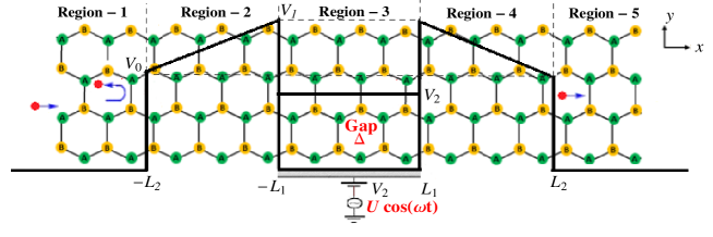
Figure 1: (color online) Representation of Dirac fermions in gapped graphene through double barriers tilting of widths $L_{2}-L_{1}$ and heights $(V_{0},V_{1})$, in the presence of a time-oscillating potential of width $2L_{1}$, amplitude $U$ and frequency $\omega$.

To provide a description of the present system, we use the Hamiltonian for one Dirac point, e.g., $K$,

$$H_{j}=v_{F}{\bm{\sigma}}\cdot\textbf{p}+V_{j}(x){\mathbb{I}}_{2}+\left[\Delta\sigma_{z}+U\cos(\omega t){\mathbb{I}}_{2}\right]\Theta\left(L_{1}^{2}-x^{2}\right)$$ (1)

where ${v_{F}\approx 10^{6}}$ m/s is the Fermi velocity, $\textbf{p}=-i\hbar(\partial_{x},\partial_{y})$, ${{\bm{\sigma}}=(\sigma_{x},\sigma_{y})}$ are the Pauli matrices, ${\mathbb{I}}_{2}$ the $2\times 2$ unit matrix, and $\Theta$ is the Heaviside step function. $\Delta=mv_{F}^{2}$ represents the energy gap that results from the sublattice symmetry breaking, or that arising from the spin-orbit interaction $\Delta=\Delta_{so}$. The electrostatic potential $V(x)=V_{j}$ in each region $j$ is expressed as follows:

$$V(x)=V_{j}=\left\{\begin{array}[]{ll}\gamma Fx+V_{L},&\hbox{$L_{1}\leq|x|\leq L_{2}$}\\ V_{2},&\hbox{$|x|\leq L_{1}$}\\ 0,&\hbox{otherwise}\\ \end{array}\right.$$ (2)

with $F=\frac{V_{1}-V_{0}}{L_{2}-L_{1}}$, $V_{L}=\frac{V_{1}L_{2}-V_{0}L_{1}}{L_{2}-L_{1}}$, $\gamma=1$ stands for $x\in[-L_{2},-L_{1}]$, and $\gamma=-1$ for $x\in[L_{1},L_{2}]$. The eigenvalue equation for the spinor $\psi_{\sf j}(x,y,t)$ at $E+l\hbar\omega$, in the unit system $\hbar=1$, reads as

$$\left[{\bm{\sigma}}\cdot\textbf{p}+v_{j}(x){\mathbb{I}}_{2}+\left(\Delta_{g}\sigma_{z}+u\cos(\omega t)\right)\Theta\left(L_{1}^{2}-x^{2}\right)\right]\psi_{\sf j}(x,y,t)=(\epsilon+l\varpi)\psi_{\sf j}(x,y,t),$$ (3)

and we have define the quantities $\epsilon=\frac{E}{\upsilon_{F}}$, $\varpi=\frac{\omega}{\upsilon_{F}}$, $v_{j}=\frac{V_{j}}{v_{F}}$, $u=\frac{U}{v_{F}}$, $\Delta_{g}=\frac{\Delta}{v_{F}}$ and $\alpha=\frac{u}{\varpi}$. The system is expected to exhibit finite width W and infinite mass boundary conditions at the boundaries $y=0$ and $y=W$ [26, 27], resulting in a quantized wave vector along the $k_{y}=k_{n}$

$$k_{n}=\frac{\pi}{W}\left(n+\frac{1}{2}\right),\quad n\in\mathbb{N}$$ (4)

By considering energy conservation, we can represent the wave packet of electrons in the $j$-th region using a linear combination of wave functions that have energies $\epsilon+m\omega$. Then, after solving the eigenvalue equation, we get the eigenspinor for incident and reflection waves in region $j$=1 ($x\leq-L_{2}$)

$$\psi_{\sf 1}(x,y,t)=e^{ik_{y}y}\sum^{+\infty}_{m,l=-\infty}\left[\delta_{l,0}\left(\begin{array}[]{c}1\\ z_{l}\end{array}\right)e^{ik_{l}x}+r_{l}\left(\begin{array}[]{c}1\\ -\frac{1}{z_{l}}\end{array}\right)e^{-ik_{l}x}\right]\delta_{m,l}e^{-iv_{F}(\epsilon+m\varpi)t}$$ (5)

where $z_{l}=s_{l}\frac{k_{l}+ik_{y}}{\sqrt{k^{2}_{l}+k_{y}^{2}}}$, $s_{l}=\mbox{sgn}(\epsilon+l\varpi)$, and

$$k_{l}=s_{l}\left(\left(\epsilon+l\varpi\right)^{2}-k^{2}_{y}\right)^{\frac{1}{2}}.$$ (6)

In the transmitted region $j$=5 ($x\geq L_{2}$), we obtain the solution

$$\psi_{\sf 5}(x,y,t)=e^{ik_{y}y}\sum^{+\infty}_{m,l=-\infty}\left[t_{l}\left(\begin{array}[]{c}1\\ z_{l}\end{array}\right)e^{ik_{l}x}+b_{l}\left(\begin{array}[]{c}1\\ -\frac{1}{z_{l}}\end{array}\right)e^{-ik_{l}x}\right]\delta_{m,l}e^{-iv_{F}(\epsilon+m\varpi)t}$$ (7)

where $\{b_{l}\}$ is the null vector. In region $j$=3 ($-L_{1}\leq x\leq L_{1}$), the solution is

$$\psi_{\sf 3}(x,y,t) = e^{ik_{y}y}\sum^{m,l=+\infty}_{m,l=-\infty}\left[a_{l}^{j}\left(\begin{array}[]{c}\lambda_{l}^{+}\\ \lambda_{l}^{-}z_{l}^{{}^{\prime}}\end{array}\right)e^{ik^{{}^{\prime}}_{l}x}+b_{l}^{j}\left(\begin{array}[]{c}\lambda_{l}^{+}\\ -\frac{\lambda_{l}^{-}}{z_{l}^{{}^{\prime}}}\end{array}\right)e^{-ik^{{}^{\prime}}_{l}x}\right]J_{m-l}\left(\alpha\right)e^{-iv_{F}(\epsilon+m\varpi)t}$$ (12)

where $\lambda_{l}^{\pm}=\left(1\pm\frac{\Delta_{g}}{\epsilon-v+l\varpi}\right)^{\frac{1}{2}}$, $z_{l}^{{}^{\prime}}=s_{l}^{{}^{\prime}}\frac{k_{l}^{{}^{\prime}}+ik_{y}}{\sqrt{k_{l}^{{}^{\prime}}+k_{y}^{2}}}$, $s_{l}^{{}^{\prime}}=\mbox{sgn}(\epsilon+l\varpi-v)$, $J_{m}\left(\frac{u}{\varpi}\right)$ is the Bessel function, and the wave vector is given by

$$k_{l}^{{}^{\prime}}=s_{l}^{{}^{\prime}}\left(\left(\epsilon-v_{2}+l\varpi\right)^{2}-\Delta_{g}^{2}-{k_{y}}^{2}\right)^{\frac{1}{2}}.$$ (13)

In regions $j$=1, 2, 4, 5 the modulation amplitude is null, $\alpha=0$, and therefore we have we have the function $J_{m-l}(0)=\delta_{m,l}$.

In regions 2 and 4 ($L_{1}<|x|<L_{2}$), the parabolic cylinder function can be used to represent the general solution [28, 29, 8]

$$\chi_{\gamma,l}^{+}=c_{n1}D_{\nu_{n}-1}\left(Q_{\gamma,l}\right)+c_{n2}D_{-\nu_{n}}\left(-Q^{*}_{\gamma,l}\right)$$ (14)

where $F=v_{F}\varrho$, $\nu_{n}=\frac{ik_{y}^{2}}{2\varrho}$, $\epsilon_{l}=\epsilon+l\varpi-v_{1}$ and $Q_{\gamma,l}(x)=\sqrt{\frac{2}{\varrho}}e^{i\pi/4}\left(\gamma\varrho x+\epsilon_{l}\right)$, $c_{n1}$ and $c_{n2}$ are constants. The second spinor component can be derived as

$$\chi_{\gamma,l}^{-}=-\frac{c_{n2}}{k_{y}}\left[2(\epsilon_{l}+\gamma\varrho x)D_{-\nu_{n}}\left(-Q^{*}_{\gamma,l}\right)+\sqrt{2\varrho}e^{i\pi/4}D_{-\nu_{n}+1}\left(-Q^{*}_{\gamma,l}\right)\right]-\frac{c_{n1}}{k_{y}}\sqrt{2\varrho}e^{-i\pi/4}D_{\nu_{n}-1}\left(Q_{\gamma,l}\right).$$ (15)

Now, by defining the components $\varphi_{\gamma,l}^{+}(x)=\chi_{\gamma,l}^{+}+i\chi_{\gamma,l}^{-}$ and $\varphi_{\gamma,l}^{-}(x)=\chi_{\gamma,l}^{+}-i\chi_{\gamma,l}^{-}$, yield the eigenspinors solution of (3) in the form provided below

$$\psi_{\sf j}(x,y,t) = e^{ik_{y}y}\sum^{m,l=+\infty}_{m,l=-\infty}\left[a_{l}^{j}\left(\begin{array}[]{c}\eta^{+}_{\gamma,l}(x)\\ \eta^{-}_{\gamma,l}(x)\\ \end{array}\right)e^{ik_{y}y}+b_{l}^{j}\left(\begin{array}[]{c}\xi^{+}_{\gamma,l}(x)\\ \xi^{-}_{\gamma,l}(x)\\ \end{array}\right)\right]J_{m-l}\left(\alpha\right)e^{-iv_{F}(\epsilon+m\varpi)t}$$ (20)

and we have set the functions

$$\eta^{\pm}_{\gamma,l}(x)=D_{\nu_{n}-1}\left(Q_{\gamma,l}\right)\mp\frac{1}{k_{y}}\sqrt{2\varrho}e^{i\pi/4}D_{\nu_{n}}\left(Q_{\gamma,l}\right)$$ (21)

$$\xi^{\pm}_{\gamma,l}(x)=\pm\frac{1}{k_{y}}\sqrt{2\varrho}e^{-i\pi/4}D_{-\nu_{n}+1}\left(-Q_{\gamma,l}^{*}\right)\pm\frac{1}{k_{y}}\left(-2i\epsilon_{0}\pm k_{y}-\gamma 2i\varrho x\right)D_{-\nu_{n}}\left(-Q_{\gamma,l}^{*}\right)$$ (22)

where $\gamma=\pm 1$. We will see in the forthcoming analysis how the above mathematical tools can be employed to achieve our goals.

III Transmissions for sidebands

It is important to remember that as Dirac electrons travel through a region with a time-varying potential, they can transfer energy quanta to the oscillating field. This results in transitions from the central band to sidebands (channels) at energies $\epsilon\pm m\varpi$ $(m=0,1,\cdots)$ and therefore generates transmission channels, which we have to determine. Indeed, if we recognize that ${e^{imv_{F}\varpi t}}$ are mutually perpendicular, we can derive a set of equations based on the boundary conditions at $x=-L_{2}$:

$$\delta_{m,0}e^{-\textbf{\emph{i}}k_{m}L_{2}}+r_{m}e^{\textbf{\emph{i}}k_{m}L_{2}}=\sum^{l=\infty}_{l=-\infty}\left(a^{2}_{l}\eta_{1,l}^{+}(-L_{2})+b^{2}_{l}\xi_{1,l}^{+}(-L_{2})\right)\delta_{m,l}$$ (23)

$$\delta_{m,0}z_{m}e^{-\textbf{\emph{i}}k_{m}L_{2}}-b_{m}^{1}\frac{1}{z_{m}}e^{\textbf{\emph{i}}k_{m}L_{2}}=\sum^{l=\infty}_{l=-\infty}\left(a^{2}_{l}\eta_{1,l}^{-}(-L_{2})+b^{2}_{l}\xi_{1,l}^{-}(-L_{2})\right)\delta_{m,l}$$ (24)

$x=-L_{1}$:

$$a^{2}_{l}\eta_{1,m}^{+}(-L_{1})+b^{2}_{l}\xi_{1,m}^{+}(-L_{1})=\sum^{l=\infty}_{l=-\infty}\left(a^{3}_{l}\lambda_{l}^{+}e^{-ik_{l}^{{}^{\prime}}L_{1}}+b^{3}_{l}\lambda_{l}^{+}e^{ik_{l}^{{}^{\prime}}L_{1}}\right)J_{m-l}\left(\alpha\right)$$ (25)

$$a^{2}_{l}\eta_{1,m}^{-}(-L_{1})-b^{2}_{l}\xi_{1,m}^{-}(-L_{1})=\sum^{l=\infty}_{l=-\infty}\left(a^{3}_{l}\lambda_{l}^{-}z_{l}^{{}^{\prime}}e^{-ik_{l}^{{}^{\prime}}L_{1}}-b^{3}_{l}\lambda_{l}^{-}\frac{1}{z_{l}^{{}^{\prime}}}e^{ik_{l}^{{}^{\prime}}L_{1}}\right)J_{m-l}\left(\alpha\right)$$ (26)

$x=L_{1}$:

$$a^{4}_{l}\eta_{-1,m}^{+}(L_{1})+b^{4}_{l}\xi_{-1,m}^{+}(L_{1})=\sum^{l=\infty}_{l=-\infty}\left(a^{3}_{l}\lambda_{l}^{+}e^{ik_{l}^{{}^{\prime}}L_{1}}+b^{3}_{l}\lambda_{l}^{+}e^{-ik_{l}^{{}^{\prime}}L_{1}}\right)J_{m-l}\left(\alpha\right)$$ (27)

$$a^{4}_{l}\eta_{-1,m}^{-}(L_{1})-b^{4}_{l}\xi_{-1,m}^{-}(L_{1})=\sum^{l=\infty}_{l=-\infty}\left(a^{3}_{l}\lambda_{l}^{-}z_{l}^{{}^{\prime}}e^{ik_{l}^{{}^{\prime}}L_{1}}-b^{3}_{l}\lambda_{l}^{-}\frac{1}{z_{l}^{{}^{\prime}}}e^{-ik_{l}^{{}^{\prime}}L_{1}}\right)J_{m-l}\left(\alpha\right)$$ (28)

and at $x=L_{2}$:

$$t_{m}e^{\textbf{\emph{i}}k_{m}L_{2}}+b_{m}^{5}e^{-\textbf{\emph{i}}k_{m}L_{2}}=\sum^{l=\infty}_{l=-\infty}\left(a^{4}_{l}\eta_{-1,l}^{+}(L_{2})+b^{4}_{l}\xi_{-1,l}^{+}(L_{2})\right)\delta_{m,l}$$ (29)

$$t_{m}z_{m}e^{\textbf{\emph{i}}k_{m}L_{2}}-b_{m}^{5}\frac{1}{z_{m}}e^{-\textbf{\emph{i}}k_{m}L_{2}}=\sum^{l=\infty}_{l=-\infty}\left(a^{4}_{l}\eta_{-1,l}^{-}(L_{2})+b^{4}_{l}\xi_{-1,l}^{-}(L_{2})\right)\delta_{m,l}.$$ (30)

We can write (29-30) in matrix form

$$\left(\begin{array}[]{c}\Xi_{1}\\ \Xi_{1}^{{}^{\prime}}\\ \end{array}\right)=\left(\begin{array}[]{cc}{\mathbb{M}_{11}}&{\mathbb{M}_{12}}\\ {\mathbb{M}_{21}}&{\mathbb{M}_{22}}\\ \end{array}\right)\left(\begin{array}[]{c}\Xi_{5}\\ \Xi_{5}^{{}^{\prime}}\\ \end{array}\right)={\mathbb{M}}\left(\begin{array}[]{c}\Xi_{5}\\ \Xi_{5}^{{}^{\prime}}\\ \end{array}\right)$$ (39)

where ${\mathbb{M}}={\mathbb{M}(1,2)}\cdot{\mathbb{M}(2,3)}\cdot{\mathbb{M}(3,4)}\cdot{\mathbb{M}(4,5)}$ is the transfer matrix such that ${\mathbb{M}(j,j+1)}$ connect the wave functions between the $j$-th and $(j+1)$-th regions

$${\mathbb{M}(1,2)}=\left(\begin{array}[]{cc}{\mathbb{N}_{1}^{+}}&{\mathbb{N}_{1}^{-}}\\ {\mathbb{L}_{1}^{+}}&{\mathbb{L}_{1}^{-}}\\ \end{array}\right)^{-1}\left(\begin{array}[]{cc}{\mathbb{C}_{1}^{+}}&{\mathbb{G}_{1}^{+}}\\ {\mathbb{C}_{1}^{-}}&{\mathbb{G}_{1}^{-}}\\ \end{array}\right),\quad{\mathbb{M}(2,3)}=\left(\begin{array}[]{cc}{\mathbb{Y}_{1}^{+}}&{\mathbb{Q}_{1}^{+}}\\ {\mathbb{Y}_{1}^{-}}&{\mathbb{Q}_{1}^{-}}\\ \end{array}\right)^{-1}\left(\begin{array}[]{cc}{\mathbb{D}_{1}^{+}}&{\mathbb{D}_{1}^{-}}\\ {\mathbb{F}_{1}^{+}}&{\mathbb{F}_{1}^{-}}\\ \end{array}\right)$$ (48)

$${\mathbb{M}(3,4)}=\left(\begin{array}[]{cc}{\mathbb{D}_{-1}^{+}}&{\mathbb{D}_{-1}^{-}}\\ {\mathbb{F}_{-1}^{+}}&{\mathbb{F}_{-1}^{-}}\\ \end{array}\right)^{-1}\left(\begin{array}[]{cc}{\mathbb{Y}_{-1}^{+}}&{\mathbb{Q}_{-1}^{+}}\\ {\mathbb{Y}_{-1}^{-}}&{\mathbb{Q}_{-1}^{-}}\\ \end{array}\right),\quad{\mathbb{M}(4,5)}=\left(\begin{array}[]{cc}{\mathbb{C}_{-1}^{+}}&{\mathbb{G}_{-1}^{+}}\\ {\mathbb{C}_{-1}^{-}}&{\mathbb{G}_{-1}^{-}}\\ \end{array}\right)^{-1}\left(\begin{array}[]{cc}{\mathbb{N}_{-1}^{+}}&{\mathbb{N}_{-1}^{-}}\\ {\mathbb{L}_{-1}^{+}}&{\mathbb{L}_{-1}^{-}}\\ \end{array}\right)$$ (57)

with the elements

$$\left({\mathbb{N}_{\gamma}^{\pm}}\right)_{m,l}=e^{\mp\gamma ik_{m}L_{2}}\delta_{m,l}$$ (58)

$$\left({\mathbb{L}_{\gamma}^{\pm}}\right)_{m,l}=\pm z_{m}^{\pm 1}e^{\mp\gamma ik_{m}L_{2}}\delta_{m,l}$$ (59)

$$\left({\mathbb{C}_{\gamma}^{\pm}}\right)_{m,l}=\eta_{\gamma,m}^{\pm}(-\gamma L_{2})\delta_{m,l}$$ (60)

$$\left({\mathbb{G}_{\gamma}^{\pm}}\right)_{m,l}=\xi_{\gamma,m}^{\pm}(-\gamma L_{2})\delta_{m,l}$$ (61)

$$\left({\mathbb{Y}_{\gamma}^{\pm}}\right)_{m,l}=\eta_{\gamma,m}^{\pm}(-\gamma L_{1})\delta_{m,l}$$ (62)

$$\left({\mathbb{Q}_{\gamma}^{\pm}}\right)_{m,l}=\xi_{\gamma,m}^{\pm}(-\gamma L_{1})\delta_{m,l}$$ (63)

$$\left({\mathbb{D}_{\gamma}^{\pm}}\right)_{m,l}=\lambda^{+}e^{\mp\gamma ik_{l}^{{}^{\prime}}L_{1}}J_{m-l}\left(\alpha\right)$$ (64)

$$\left({\mathbb{F}_{\gamma}^{\pm}}\right)_{m,l}=\pm\lambda^{-}(z_{l}^{{}^{\prime}})^{\pm 1}e^{\mp\gamma ik_{l}^{{}^{\prime}}L_{1}}J_{m-l}\left(\alpha\right)$$ (65)

Here $\Xi_{1}=\{a_{m}^{1}\}=\{\delta_{m,0}\}$, $\tau\in\{1,2\}$, $\Xi_{1}^{{}^{\prime}}=\{b_{m}^{1}\}=\{r_{m}\}$ represents the reflections, $\Xi_{5}^{{}^{\prime}}=\{b_{m}^{5}\}$ denotes a null vector, $\Xi_{5}=\{a_{m}^{5}\}=\{t_{m}\}$ represents the transmissions. Consequently, we end up with

$$\Xi_{5}={\mathbb{M}}_{11}^{-1}\cdot\Xi_{1}.$$ (66)

To find the minimum number of sidebands, we need to evaluate the strength of the oscillating potential, which can be expressed as $N>\alpha$ [30]. Consequently, we can simplify the infinite series for transmission by considering only a finite number of terms. Specifically, we can restrict the series to terms ranging from $-N$ to $N$ as reported in [31, 32, 25, 33, 34]. Therefore, we can express the series as follows:

$$t_{-N+k}={\mathbb{M}}_{11}^{-1}\left[k+1,N+1\right],\qquad k=0,1,\cdots,2N$$ (67)

In getting the transmission $T_{l}$ and reflection $R_{l}$ probabilities, we consider the current density $J$ associated with the present system that can be calculated as

$$J=v_{F}\psi^{\dagger}\sigma_{x}\psi$$ (68)

giving rise to the incident $J_{\sf{inc,0}}$, transmitted $J_{{\sf{tra}},l}$, and reflected $J_{{\sf{ref}},l}$, knowing that

$$T_{l}=\frac{|J_{{\sf{tra}},l}|}{|J_{{\sf{inc}},0}|},\quad R_{l}=\frac{|J_{{\sf{ref}},l}|}{|J_{\sf{inc,0}}|}.$$ (69)

Recall that $T_{l}$ characterize the scattering of an electron with an incident energy $\epsilon$ in region 1, into the sidebands with energies $\epsilon+l\varpi$ in region 5. After some algebras, we obtain

$$T_{l}=\frac{k_{l}}{k_{0}}|t_{l}|^{2},\quad R_{l}=\frac{k_{l}}{k_{0}}|r_{l}|^{2}.$$ (70)

Due to numerical challenges in the forthcoming analysis, we will truncate (67) and keep only the terms associated with the central and first two sidebands, specifically $l=0,\pm 1$. From here, we can proceed as previously done to determine the transmission amplitudes

$$t_{-1}={\mathbb{M}}_{11}^{-1}[1,2],\quad t_{0}={\mathbb{M}}_{11}^{-1}[2,2],\quad t_{1}={\mathbb{M}}_{11}^{-1}[3,2].$$ (71)

At low energies, this approximation can be established because single photon process are more likely to occur than two- and higher-photon processes. We will conduct a numerical analysis to better understand the obtained results and highlight the behavior of the system. To accomplish this, we will concentrate on a limited number of channels and select various configurations of the physical parameters.

IV Discussion of numerical results

The following section displays the numerical outcomes for the transmission coefficients. These results are exhibited in Figs. (2-7) for multiple parameter values, including $\epsilon$, $v_{1}$, $v_{2}$, $\Delta_{g}$, $L_{1}$, and $L_{2}$. Figs. 2 and 3 depict the transmission probability solely for the central band $T_{0}$, as a function of energy $\epsilon$, with $\alpha=0$, $L_{1}$ taking values of 0.1 (blue line), 0.4 (green line), and 1.2 (red line), while $L_{2}$ is fixed at 2.5, $\Delta_{g}$ is 4, and $k_{y}$ is 2. The double barriers tilting case is considered, where $v_{2}<v_{0}<v_{1}$, $v_{0}<v_{1}<v_{2}$, and $v_{0}<v_{2}<v_{1}$. The transmission for both situations is graphed in Fig. 2. In Fig. 2a, it can be observed that the transmission through a graphene double barrier tilting with $v_{2}<v_{0}<v_{1}$ is characterized by six energy zones. The zone with a higher effective mass is defined as the first zone and is characterized by $\epsilon<ky$. The second zone, which is associated with resonances, is referred to as the lower Klein energy zone and is defined by $k_{y}<\epsilon<v_{2}-(k_{y}+\Delta_{g}/2)$. In this zone, there are specific energies where full transmission occurs despite the particle energy being less than the barrier height. Additionally, the oscillations are reduced, which suggests that Klein tunneling may be suppressed as $L_{1}$ increases. Transmission is nearly zero within the third zone, which is characterized by $v_{2}-(k_{y}+\Delta_{g}/2)<\epsilon<v_{2}+(k_{y}+\Delta_{g}/2)$. The fourth zone, defined by $v_{2}+(k_{y}+\Delta_{g}/2)<\epsilon<v_{0}$, is characterized by transmission oscillations around the total transmission value. Within the fifth zone, which is defined by $v_{0}<\epsilon<v_{1}$, the transmission exhibits resonance peaks that correspond to the bound states associated with the double barrier tilting. The sixth zone is $\epsilon>v_{1}$, where the transmission converges to unity and contains oscillations. In contrast to the case $v_{0}<v_{1}<v_{2}$, the behaviors of some zones in Fig. 2a are completely reversed, such as the window zone. Fig. 2c shows the behavior of the transmission for the case $v_{0}<v_{2}<v_{1}$, which is completely different from Figs. 2a and 2b. However, as $L_{1}$ increases, the number of oscillations of transmission increases for $k_{y}<\epsilon<v_{2}-(k_{y}+\Delta_{g}/2)$ and $\epsilon>v_{2}-(k_{y}+\Delta_{g}/2)$ and decreases for $v_{2}-(k_{y}+\Delta_{g}/2)<\epsilon<v_{2}+(k_{y}+\Delta_{g}/2)$. The impact of barrier width on transmission is also noticeable, as an increase in $d_{1}$ results in a decrease in the minimum transmission within the intermediate zones $v_{0}<\epsilon<v_{1}$, and an increase in the number of oscillations.

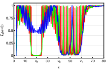
(a)

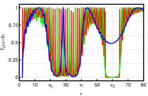
(b)

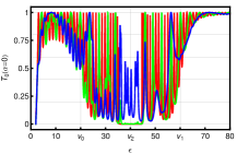
(c)

Figure 2: (color online) Transmission $T_{0}(\alpha=0)$ versus incident energy $\epsilon$ for $\Delta_{g}=4$, $k_{y}=2$, $L_{2}=2.5$, and $L_{1}=0.1$ (blue line), $L_{1}=0.4$ (green line), $L_{1}=1.2$ (red line). (a): $v_{0}=40$, $v_{1}=60$, $v_{2}=20$, (b): $v_{0}=20$, $v_{1}=40$, $v_{2}=60$, and (c): $v_{0}=20$, $v_{1}=60$, $v_{2}=40$.

To illustrate the significance of our findings, we present two cases depicted in Fig. 3, which depend on the choice of barrier heights $(v_{0},v_{1},v_{2})$. Specifically, Fig. 3a displays a double square barrier scenario with $v_{2}=20$ and $(v_{0}\approx v_{1}=60)$. The transmission in the Klein zone is not depicted, and the transmission oscillates around a minimum before behaving similarly to the results in Fig. 2a. However, the number of peaks decreases for double square barriers, while it increases for double barriers with tilting. On the other hand, Fig. 3b shows the case of a single square barrier with $v_{0}\approx v_{1}=v_{2}=40$. We investigate how the interplay between the effects of distributed scatters in a barrier and barrier tilting affects the tunneling transport of Dirac electrons in graphene. We observe that the tilting and position of the scattering within the barriers play a crucial role in controlling the peak of tunneling resistance and switching it to a cusp with the presence of a mid-barrier-embedded scatter when the incident energy reaches the Dirac point in a barrier. Furthermore, a continuously distributed scatter suppresses constructive interference around the Dirac point, converting a cusp into a peak in the tunneling resistance as the incident energy of electrons varies. In contrast to a single scatter, a continuous distribution within a barrier enhances unimpeded incoherent tunneling for head-on collisions and greatly suppresses skew collisions as the barrier tilting field increases [35].

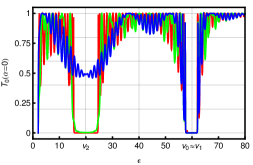
(a)

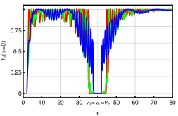
(b)

Figure 3: (color online) The same as in Fig. 2 but with (a): $v_{0}\approx v_{1}=60$, $v_{2}=20$, and (b): $v_{0}\approx v_{1}=v_{2}=40$.

Let us explore the effects of introducing a time-varying potential with a sinusoidal oscillation of amplitude $u_{1}$ and frequency $\omega$ ($\alpha\neq 0$) in the intermediate region, where its height is oscillating around $v_{2}$. In Fig. 4, we show the transmission probabilities for the central band ($T_{0}$ in blue) and the first two sidebands ($T_{-1}$ in green and $T_{1}$ in red) versus the incident energy $\epsilon$, with the same as in Fig. 2. As anticipated, the transmissions are currently dispersed across both the central band and the sidebands. In addition, the utmost transmission via the oscillating barrier is dependent on the value of $\alpha$.

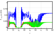
(a)

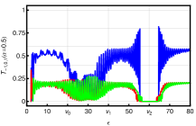
(b)

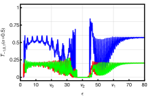
(c)

Figure 4: (color online) Transmissions versus incident energy $\epsilon$ for $\alpha=0.5$, $\Delta_{g}=4$, $k_{y}=2$, $L_{1}=1.5$, and $L_{2}=2.5$. (a): $v_{0}=20$, $v_{1}=40$, $v_{2}=60$, (b): $v_{0}=40$, $v_{1}=60$, $v_{2}=20$, and (c): $v_{0}=20$, $v_{1}=60$, $v_{2}=40$. $T_{-1}$ (green line), $T_{0}$ (blue line) and $T_{1}$ (red line).

Fig. 5 depicts the central transmission band $T_{0}$ (blue), and the first two sidebands $T_{-1}$ (red) and $T_{1}$ (green) as a function of the energy $\epsilon$. We consider a system with $L_{1}=1.5$, $L_{2}=2.5$, $\Delta_{g}=4$, $k_{y}=2$, $v_{0}=0$, $v_{1}=40$, and $v_{2}=60$. We investigate the effect of static and oscillating barriers with $\alpha=0$ (panel a), $\alpha=0.4$ (panel b), and $\alpha=0.98$ (panel c). Due to the sinusoidal and longitudinal vibrations of the time-oscillating barrier in the $x$-direction of Dirac fermions, with an amplitude of $u_{1}$ and frequency of $\omega$, the effective mass changes from $k_{y}$ to $k_{y}\pm\omega$. For small values of $\alpha$, $T_{0}$ dominates, as shown in Fig. 5a, but as $\alpha$ increases, $T_{0}$ decreases, and $T_{-1}$ as well as $T_{1}$ increase, as seen in Fig. 5b. In Fig. 5c, we see that transmissions of the two first sidebands ($l=\pm 1$) dominate. In conclusion, we notice that increasing $\alpha$ leads to a decrease in $T_{0}$ and an increase in both $T_{\pm 1}$.

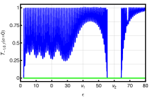
(a)

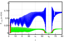
(b)

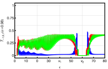
(c)

Figure 5: (color online) The same as in Fig. 4 but with $v_{0}=0$, $v_{1}=40$, $v_{2}=60$. (a): $\alpha=0$ (b): $\alpha=0.4$, and (c): $\alpha=0.98$.

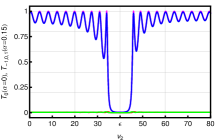
(a)

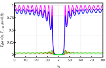
(b)

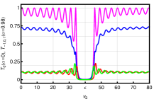
(c)

Figure 6: (color online) Transmissions versus potential $v_{2}$ for $L_{1}=0.4$, $L_{2}=0.8$, $\Delta_{g}=4$, $k_{y}=2$, $v_{0}=50$, $v_{1}=70$, $\epsilon=60$, $T_{0}$ (magenta color), $T_{-1}$ (green line), $T_{0}$ (blue line), and $T_{1}$ (red line). (a): $\alpha=0.15$, (b): $\alpha=0.5$, and (c): $\alpha=0.98$.

Fig. 6 displays the transmission probabilities versus potential $v_{2}$ with fixed parameters $L_{1}=0.4$, $L_{2}=0.8$, $\Delta_{g}=4$, $k_{y}=2$, $v_{0}=50$, $v_{1}=70$, and $\epsilon=60$. Here, the transmission probability $T_{0}$ (magenta) for the static barrier is shown in comparison to the transmission probabilities for the oscillating barrier with $\alpha\neq 0$. Specifically, the transmissions for the central band $T_{0}$ (blue) and the first two sidebands $T_{-1}$ (green) and $T_{1}$ (red) are shown for oscillating barriers with $\alpha=0.15$ (a), $\alpha=0.5$ (b), and $\alpha=0.98$ (c). We observe that the increase of $\alpha$ decreases $T_{0}$ but increases $T_{-1}$ and $T_{1}$. Notably, the value of $\alpha$ plays a crucial role in determining the transmission probabilities for the sidebands. The two sidebands’ transmissions are located near the axis of symmetry, where the central transmission strictly ranges between zero and one. This ensures that the sum of all transmissions does not exceed one, and both sidebands become symmetrical with respect to the opposite side of the axis of symmetry.

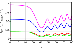
(a)

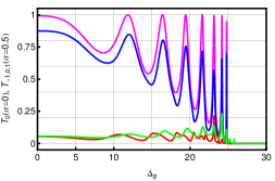
(b)

Figure 7: (color online) (a): Transmissions versus potential $v_{1}$ for $L_{1}=1.5$, $L_{2}=2.5$, $\Delta_{g}=4$ and $k_{y}=2$, $v_{0}=0$, $v_{2}=60$, $\epsilon=30$. (b): Transmissions versus energy gap $\Delta_{g}$ for $L_{1}=0.5$, $L_{2}=1.5$, $k_{y}=1$, $v_{0}=0$, $v_{1}=50$, $v_{2}=40$, and $\epsilon=15$. $T_{0}(\alpha=0)$ (magenta line), $T_{-1}(\alpha=0.5)$ (green line), $T_{0}(\alpha=0.5)$ (blue line), and $T_{1}(\alpha=0.5)$ (red line).

In Fig. 7a, we depict the transmission probabilities $T_{0,\pm 1}(\alpha=0.5)$ versus potential $v_{1}$ for $L_{1}=1.5$, $L_{2}=2.5$, $\Delta_{g}=4$, $k_{y}=2$, $v_{0}=0$, $v_{2}=60$, and $\epsilon=30$. We see that $T_{0}$ exhibits a sharp decline for $v_{1}>\epsilon+lw-(2k_{y}+\Delta_{g})$, reaching a relative minimum before oscillating and increasing again. In Fig. 7b, we show the transmission probabilities versus energy gap $\Delta_{g}$ for $L_{1}=0.5$, $L_{2}=1.5$, $k_{y}=1$, $v_{0}=0$, $v_{1}=50$, $v_{2}=40$, and $\epsilon=15$. The maximum value of $T_{0}$ (magenta) is unity for $\alpha=0$. However, for $\alpha=0.5$, the maximum value of $T_{0}$ (blue) decreases, while the sideband transmissions $T_{-1}$ (green) and $T_{1}$ (red) increase. We observe that the sum of the three transmissions $T_{0}(\alpha=0.5)$, $T_{-1}(\alpha=0.5)$, and $T_{1}(\alpha=0.5)$ converges towards unity. Moreover, it should be noted that specific energy gaps completely block transmission. In fact, when the condition $\Delta_{g}>|\epsilon+lw-v_{2}|$ is satisfied, any incoming state is reflected.

V Conclusion

We have studied the tunneling effect of electrons in gapped graphene passing through tilted double barriers and time-oscillating potential. More precisely, we have investigated how the transmission probabilities vary with respect to the incident energy, potential heights $v_{2}$ and $v_{1}$, energy gap, and incident angle. The results show that the tilting of the barriers and the position of the scatterers are crucial in tuning the peak of tunneling when the incident energy approaches the Dirac point. Moreover, the distributed scatterers effectively suppress the constructive interference around the Dirac point, which causes a change from a cusp to a peak in the tunneling resistance as a function of the incident energy.

We have demonstrated that the oscillating barrier can play a crucial role in adjusting the transmission probabilities. Indeed, the time-varying potential induces additional sidebands in the transmission probability at energies of $\epsilon+l\hbar\omega$, arising from photon emission or absorption within the oscillating barrier. We have calculated the transmission probabilities for the central band and the first sidebands. Our findings indicate that $T_{0}$ in the oscillating barrier decreases with increasing $\alpha$, whereas $T_{-1}$ and $T_{1}$ increase. It is worth highlighting that the transmission probabilities for the sidebands through a graphene barrier tilted in a time-periodic potential are significantly influenced by the value of $\alpha$.

References

[1] A. K. Geim and K. S. Novoselov, Nat. Mater. 6, 183 (2007).
[2] K. S. Novoselov, A. K. Geim, S. V. Morozov, D. Jiang, Y. Zhang, S. V. Dubonos, I. V. Grigorieva, and A. A. Firsov, Science 306,
666 (2004).
[3] A. H. Castro Neto, F. Guinea, N. M. R. Peres, K. S. Novoselov, and A. K. Geim, Rev. Mod. Phys. 81, 109 (2009).
[4] M. Ramezani Masir, P. Vasilopoulos, and F. M. Peeters, New J. Phys. 11, 095009 (2009).
[5] A. Jellal and A. El Mouhafid, J. Phys. A: Math. Theo. 44,
015302 (2011).
[6] E. B. Choubabi, M. El Bouziani, and A. Jellal, Int. J. Geom.
Meth. Mod. Phys. 7, 909 (2010).
[7] H. Bahlouli, E. B. Choubabi, A. Jellal, and M. Mekkaoui, J. Low
Temp. Phys. 169, 51 (2012).
[8] H. Bahlouli, E. B. Choubabi, A. El Mouhafid, and A. Jellal,
Solid State Commun. 151, 1309 (2011).
[9] M. Mekkaoui, R. El Kinani, and A. Jellal, Mater. Res. Express 6, 085013 (2019).
[10] Y. Fattasse, M. Mekkaoui, and A. Jellal, Eur.
Phys. J. B 95 (2022).
[11] A. El Mouhafid
and A. Jellal, J. Low Temp. Phys. 173, 264 (2013).
[12] M. Mekkaoui, A. Jellal, and H. Bahlouli, Physica E 111, 218 (2019).
[13] A. H. Dayem and R. J. Martin, Phys. Rev. Lett. 8, 246 (1962).
[14] P. K. Tien and J. P. Gordon, Phys. Rev. 129, 647 (1963).
[15] M. Moskalets and M. Buttiker, Phys. Rev. B 66, 035306 (2002).
[16] M. Wagner, Phys. Rev. B 49, 16544 (1994); ibid, Phys. Rev. A 51, 798 (1995); ibid, Phys. Rev. Lett. 76, 4010 (1996); ibid, Phys. Stat. Sol. (b) 204, 328 (1997); ibid, Phys. Rev. B 57,
11899 (1998), M. Wagner and W. Zwerger, Phys. Rev. B 55, 10217, (1997).
[17] P. Jiang, A. F. Young, W. Chang, P. Kim, L. W. Engel, and
D. C. Tsui, Appl. Phys. Lett. 97, 062113 (2010).
[18] H. L. Calvo, H. M. Pastawski, S. M Wagner, Phys. Rev. B 49, 16544 (1994); M Wagner, Phys. Rev. A 51, 798 (1995); M
Wagner, Phys. Rev. Lett. 76, 4010 (1996); M. WagnEur. Phys.
Lett.er, Phys. Stat. Sol. (b) 204, 328 (1997);
M. Wagner and W. Zwerger, Phys. Rev. B 55, 10217, (1997); M. Wagner, Phys. Rev. B 57,
11899 (1998-I).Roche and L. E. F. Foa
Torres, Appl. Phys. Lett. 98, 232103 (2011).
[19] P. San-Jose, E. Prada, H. Schomerus and S. Kohler,
Appl. Phys. Lett. 101, 153506 (2012).
Eur. Phys.Eur. Phys.
Lett.
Lett.
[20] S. E. Savel’ev and A. S. Alexandrov, Phys. Rev. B
84, 035428 (2011).
[21] S. E. Savel’ev, W. Hausler and P. Hanggi, Phys. Rev.
Lett. 109, 226602 (2012).
[22]T. L. Liu, L. Chang and C. S. Chu, Phys. Rev. B 88, 195419
(2013).
[23] M. V. Fistul and K. B. Efetov, Phys. Rev. Lett. 98,
256803 (2007).
[24] E. Grichuk and E. Manykin, Eur. Phys. J. B 86, 210 (2013).
[25] E. B. Choubabi, A. Jellal, and M. Mekkaoui, Eur. Phys. J. B 92, 85
(2019).
[26] J. Tworzydlo, B. Trauzettel, M. Titov, A. Rycerz, and C. W. J.
Beenakker, Phys. Rev. Lett. 96, 246802 (2006).
[27] M. V. Berry and R. J. Modragon, Proc. R. Soc. London Ser. A 412,
53 (1987).
[28] M. Abramowitz and I. Stegum, Handbook of Integrabls,
Series
and Products (Dover, New York, 1956).
[29] L. Gonzalez-Diaz and V. M. Villalba, Phys. Lett. A 352, 202
(2006).
[30] M. Ahsan Zeb, K. Sabeeh and M. Tahir, Phys. Rev. B 78,
165420 (2008).
[31] A. Jellal, M. Mekkaoui, E. B. Choubabi, and H. Bahlouli, Eur.
Phys. J. B 87 (2014).
[32] M. Mekkaoui, E. B. Choubabi, A. Jellal, and
H. Bahlouli, Mater. Res. Express 4, 035002 (2017).
[33] B. Lemaalem, M. Mekkaoui, A. Jellal, and H. Bahlouli, EPL 129, 27001 (2020).
[34] M. Mekkaoui, A. Jellal, and H. Bahlouli, Physica E. 127, 114502
(2021).
[35] Farhana Anwar, Andrii Iurov, Danhong Huang, Godfrey Gumbs, and Ashwani
Sharma, Phys. Rev. B 101, 115424 (2020).