Exploring the axion potential and axion walls in dense quark matter

Abstract

We study the potential of the Quantum Chromodynamics axion in hot and/or dense quark matter, within a Nambu-Jona-Lasinio-like model that includes the coupling of the axion to quarks. Differently from previous studies, we implement local electrical neutrality and $\beta-$equilibrium, which are relevant for the description of the quark matter in the core of compact stellar objects. Firstly we compute the effects of the chiral crossover on the axion mass and self-coupling. We find that the low energy properties of axion are very sensitive to the phase transition of Quantum Chromodynamics, in particular, when the bulk quark matter is close to criticality. Then, for the first time in the literature we compute the axion potential at finite quark chemical potential and study the axion domain walls in bulk quark matter. We find that the energy barrier between two adjacent vacuum states decrease in the chirally restored phase: this results in a lower surface tension of the walls. Finally, we comment on the possibility of production of walls in dense quark matter.

I Introduction

Quantum Chromodynamics (QCD) is a fundamental quantum field theory that provides a comprehensive framework for describing the strong interaction, which is characterized by a variety of remarkable features including color confinement, chiral symmetry breaking, and the $U(1)_{A}$ anomaly. QCD is invariant under gauge transformations belonging to the $SU(3)$ color group; however, gauge invariance does not forbid the term

$${\cal L}_{\theta}\propto\theta F\cdot\tilde{F}$$ (1)

in the QCD Lagrangian density. In (1), $F$ and $\tilde{F}$ denote the gluon field strength tensor and its dual respectively, while $\theta$ is a real parameter called the $\theta-$angle. A $\theta\neq 0$ would imply an explicit breaking of the charge conjugation, $C$, and parity, $P$, symmetries and QCD would not be invariant under $CP$ transformations (thereby inducing an electric dipole moment for the neutron [1]); however, there is evidence that $\theta\lesssim 10^{-11}$ [2, 3, 4, 5, 6, 7, 8]. The fact that $\theta$ is so small despite the fact that it is not forbidden by gauge invariance is called the strong $CP-$problem. In order to understand this problem it was suggested that a pseudoscalar field, $a$, exists and couples to the nontrivial gluon field configurations via the Lagrangian density

$${\cal L}_{a}=\frac{a}{f_{a}}F\cdot\tilde{F};$$ (2)

then, including the $\theta-$term (1) the $CP-$breaking Lagrangian would be

$${\cal L}_{\mathrm{CP}}=\theta F\cdot\tilde{F}+\frac{a}{f_{a}}F\cdot\tilde{F}.$$ (3)

Therefore, violations of $CP$ in strong interactions would be driven by $\theta+a/f_{a}$. The coupling of $a$ to the gluon field gives rise to a potential for $a$ itself: it was then assumed that this potential develops a minimum such that $\langle a/f_{a}+\theta\rangle=0$. Hence, the expectation value of $a$ would cancel the contributions to observables coming from the $\theta-$term in Eq. (3). This is called the Peccei-Quinn (PQ) mechanism and leads to potential solution of the strong $CP-$problem [9, 10, 11, 12, 13, 14, 15, 16]. While the PQ mechanism is quite elegant, it implies the existence of a light particle, the QCD-axion (for simplicity we refer to this particle as the axion in this article), which represents the quantum fluctuation of the $a$ field around $\langle a\rangle$. Axions are dark matter candidates [11, 17, 18, 19], they could arrange in the form of stars [20, 21, 22, 23, 24, 25, 26, 27, 28, 29, 30, 31, 32, 33, 34] and might form Bose-Einstein condensates [35, 36].

Given the wide range in temperature and density of the physical systems in which axions might play a role, it is important to know how the properties of this particle vary by changing the environment, in particular temperature and density. This is the main scope of the present study, in which we compute how the axion properties are affected by the temperature and the density of the medium, focusing in particular to temperatures and chemical potentials around the QCD chiral phase transitions.

The use of perturbative methods to study the physical properties of axions around the QCD critical temperature and/or in dense quark matter is questionable, hence it is necessary to resort to QCD-like models and effective field theories to explore physics in the moderate energy scale. A commomly used effective theory is the Chiral Perturbation Theory ($\chi$PT), which plays an important role in the study of the vacuum structure of QCD as well as the axion properties at low temperatures by means of systematically expanding the action in powers of the momenta of the lighter mesons [37, 38, 39, 40, 41, 42]. $\chi$PT shows great advantages in the low energy regimes, for example, its prediction of the topological susceptibility at zero temperature [13] is in good agreement with the lattice QCD results [43, 44, 45]. However, at high temperature and/or large density, $\chi$PT cannot be used due to the fact that it lacks information about the QCD phase transitions. Consequently, the use of a QCD-like model that is capable to accomodate axions and the QCD phase transition is very welcome.

In this study, we use the Nambu-Jona-Lasinio (NJL) model [52, 51, 50, 49, 48], to study the low energy properties of axions. The model incorporates the instanton-induced interaction that is responsible of the breaking of the $U(1)_{A}$ symmetry and is capable to describe the spontaneous breaking of chiral symmetry as well as the coupling of quarks to the axions. In comparison with previous studies, the use of the NJL model allows us to quantify the effects of the QCD phase transitions on the low-energy properties of the axion. We find that the chiral phase transition substantially affects the axion mass and self-coupling, particularly when the bulk of dense matter is close to the critical endpoint: indeed, near the critical endpoint, we find that the axion mass drops while the self-coupling is enhanced. Both trends agree with previous model studies [53, 54, 55, 56, 57].

The main novelties of our work can be summarized as follows. Firstly, we implement $\beta-$equilibrium and electrical neutrality, keeping in mind potential applications to compact stellar objects. When compared to previous works, our approach has the merit to include the effect of the chiral phase transition on the low-energy properties of the axions. Secondly, we study the axion walls [58, 59] and analyze how these could be produced in the cores of compact stellar objects. We discuss for the first time how chiral symmetry restoration in dense quark matter affects the surface tension of the walls. We then briefly discuss how these walls could form in the cores of compact stellar objects.

The plan of the article is as follows. In Section II we present in some detail the model we use to describe the coupling of the QCD axion to hot and dense quark matter. In Section III we present the results on axion mass, self-coupling, potential and walls at finite temperature and density. Finally, in Section IV we present our conclusions. Natural units $\hbar=1$, $c=1$ and $k_{B}=1$, are used throughout the article.

II The model

We work in the grand canonical ensemble formalism, using $T$ and $\mu$ as state variables, where $\mu$ denotes the quark number chemical potential. We consider quark matter of two light flavors with Lagrangian density is given by [52, 51, 50, 49, 48, 60, 61, 53, 54, 55, 56, 57]

$$\mathcal{L}=\bar{q}\left(i\hbox to0.0pt{/\hss}\partial+\hat{\mu}\gamma_{0}-m_{0}\right)q+\bar{e}\left(i\hbox to0.0pt{/\hss}\partial+\mu_{e}\gamma_{0}\right)e+\mathcal{L}_{\mathrm{int}}.$$ (4)

Here $q$ denotes the quark field carrying Dirac, color and flavor indices, while $e$ is the electron field. $m_{0}$ is the current quark mass, that we take to be equal for $u$ and $d$ quarks for simplicity. The quark chemical potential matrix is

$$\hat{\mu}=\left(\begin{array}[]{cc}\mu_{u}&0\\ 0&\mu_{d}\end{array}\right)\otimes\bm{1}_{c}$$ (5)

with $\bm{1}_{c}$ denoting the identity in color space and

$$\mu_{u}=\mu-\frac{2}{3}\mu_{e},~{}~{}~{}\mu_{d}=\mu+\frac{1}{3}\mu_{e};$$ (6)

$\mu_{d}=\mu_{u}+\mu_{e}$ in agreement with the requirement of $\beta-$equilibrium. Moreover, the interaction term is taken as [53, 54, 55, 56, 57]

$$\mathcal{L}_{\mathrm{int}} = G_{1}\left[(\bar{q}\tau_{a}q)(\bar{q}\tau_{a}q)+(\bar{q}\tau_{a}i\gamma_{5}q)(\bar{q}\tau_{a}i\gamma_{5}q)\right]$$ (7)

$$+8G_{2}\left[e^{i\frac{a}{f_{a}}}\mathrm{det}(\bar{q}_{R}q_{L})+e^{-i\frac{a}{f_{a}}}\mathrm{det}(\bar{q}_{L}q_{R})\right];$$

in particular, the second line in the above equation corresponds to the $U(1)_{A}$-breaking term that is responsible of the coupling of the QCD-axion to the quarks [62, 63]. In the above equation, $\tau_{a}$ are matrices in the flavor space with $a=0,\dots,3$; $\tau_{0}$ is the identity and $\tau_{i}$ with $i=1,2,3$ are Pauli matrices, normalized as $\mathrm{tr}(\tau_{i}\tau_{i})=\delta_{ij}/2$. The coupling constant $G_{1}$ governs the $U(1)_{A}-$invariant interaction. Similarly, $G_{2}$ regulates the strength of the $U(1)_{A}-$breaking term; the determinant in the latter is understood in the flavor space.

The thermodynamic potential at one loop has been discussed in the literature, see [53] and references therein; it reads

$$\Omega=\Omega_{\mathrm{mf}}+\Omega_{\mathrm{1-loop}}+\Omega_{e}.$$ (8)

Here we take

$$\Omega_{\mathrm{mf}} = -G_{2}(\eta^{2}-\sigma^{2})\cos(a/f_{a})+G_{1}(\eta^{2}+\sigma^{2})$$ (9)

$$-2G_{2}\sigma\eta\sin(a/f_{a}),$$

that represents the mean field contribution to $\Omega$, with $\sigma=\langle\bar{q}q\rangle$, $\eta=\langle\bar{q}i\gamma_{5}q\rangle$. Moreover,

$$\Omega_{e}=-2T\frac{4\pi}{8\pi^{3}}\left(\frac{7\pi^{4}}{180}T^{3}+\frac{\pi^{2}\mu_{e}^{2}T}{6}+\frac{\mu_{e}^{4}}{12T}\right)$$ (10)

is the contribution of the free, massless electrons. Finally, $\Omega_{\mathrm{1-loop}}$ corresponds to the quark loop contribution, given by

$$\Omega_{q} = -4N_{c}\sum_{f=u,d}\int\frac{d^{3}p}{(2\pi)^{3}}\left[\frac{E_{p}}{2}\right.$$

$$+\left.\frac{1}{2\beta}\log(1+e^{-\beta(E_{p}-\mu_{f})})(1+e^{-\beta(E_{p}+\mu_{f})})\right],$$

with $\beta=1/T$. The dispersion laws of quarks are given by

$$E_{p}=\sqrt{p^{2}+\Delta^{2}},~{}~{}~{}\Delta^{2}=(m_{0}+\alpha_{0})^{2}+\beta_{0}^{2},$$ (12)

with

$$\alpha_{0}=-2\left[G_{1}+G_{2}\cos(a/f_{a})\right]\sigma+2G_{2}\eta\sin(a/f_{a}),$$

(13)

$$\beta_{0}=-2\left[G_{1}-G_{2}\cos(a/f_{a})\right]\eta+2G_{2}\sigma\sin(a/f_{a}).$$

(14)

We notice that the first integral in the right hand side of Eq. (LABEL:eq:Om2) is ultraviolet divergent: we regularize this divergence by cutting the integration at $p=\Lambda$. The set of parameters we use is [53] $\Lambda=590$ MeV, $G_{0}\Lambda^{2}=2.435$, $G_{1}=(1-c)G_{0}$, $G_{2}=cG_{0}$, $c=0.2$, $m_{0}=6$ MeV.

The electron chemical potential is fixed for each value of the pair $(\mu,T)$ by imposing the electrical neutrality condition

$$\frac{\partial\Omega}{\partial\mu_{e}}=0.$$ (15)

This condition is important for potential applications to the core of compact stars. Moreover, the condensates are computed self-consistently by solving the gap equations

$$\frac{\partial\Omega}{\partial\sigma}=0,~{}~{}~{}\frac{\partial\Omega}{\partial\eta}=0,$$ (16)

being sure that the solution $\sigma=\bar{\sigma}$, $\eta=\bar{\eta}$ corresponds to the global minimum of $\Omega$.

III Results

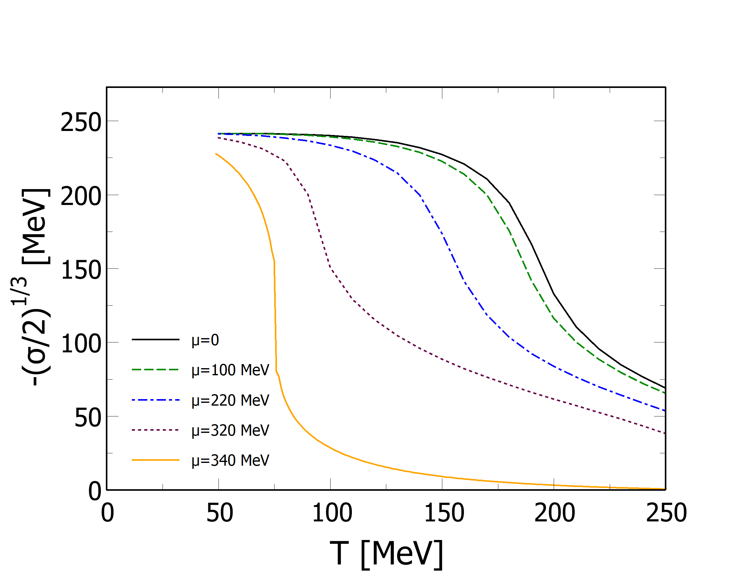
Figure 1: Chiral condensate, -$(\sigma/2)^{1/3}$, versus $T$ for several values of $\mu$ in the neutral ground state.

In Fig. 1 we plot $-(\sigma/2)^{1/3}=-(\langle\bar{u}u+\bar{d}d\rangle/2)^{1/3}$ versus $T$ for several values of $\mu$; the electron chemical potential has been computed self-consistently by solving simultaneously the gap equations (16) and the neutrality condition (15) for $a=0$. In this case the $\eta-$condensate vanishes.

We notice that for all the values of $\mu$ considered, the chiral condensate drops down in a narrow range of temperature, signaling the approximate restoration of chiral symmetry. This allows us to define a pseudo-critical temperature, $T_{c}$, as the temperature where $\sigma$ has its largest variation. $T_{c}$ drops as the chemical potential increases. In addition to this, we notice that the variation of $\sigma$ becomes sharper with $\mu$: the smooth crossover at $\mu=0$ becomes a sharp transition at at large $\mu$. This implies the existence of a critical endpoint in the phase diagram: we found it is located at $(\mu_{\mathrm{CP}},T_{\mathrm{CP}})={(336\textup{MeV},79\textup{MeV})}$. For completeness, at $T=0$ the critical chemical potential is $\mu_{C}=393$ MeV.

The axion mass and self-coupling are given by

$$m_{a}^{2}=\left.\frac{d^{2}\Omega}{da^{2}}\right|_{a=0},~{}~{}~{}\lambda_{a}=\left.\frac{d^{4}\Omega}{da^{4}}\right|_{a=0},$$ (17)

where the derivatives are total derivatives, namely they take into account that the two condensates depend on $a$, and are understood at $\sigma=\bar{\sigma}$, $\eta=\bar{\eta}$, where $\bar{\sigma}$ and $\bar{\eta}$ are the values of the condensates that minimize $\Omega$. Since the condensates depend on $a$, the neutrality condition (15) has to be computed by taking into account this dependence as well. Thus

$$\frac{d}{da}=\frac{\partial}{\partial a}+\frac{\partial\sigma}{\partial a}\frac{\partial}{\partial\sigma}+\frac{\partial\eta}{\partial a}\frac{\partial}{\partial\eta},$$ (18)

and so on for the higher derivatives.

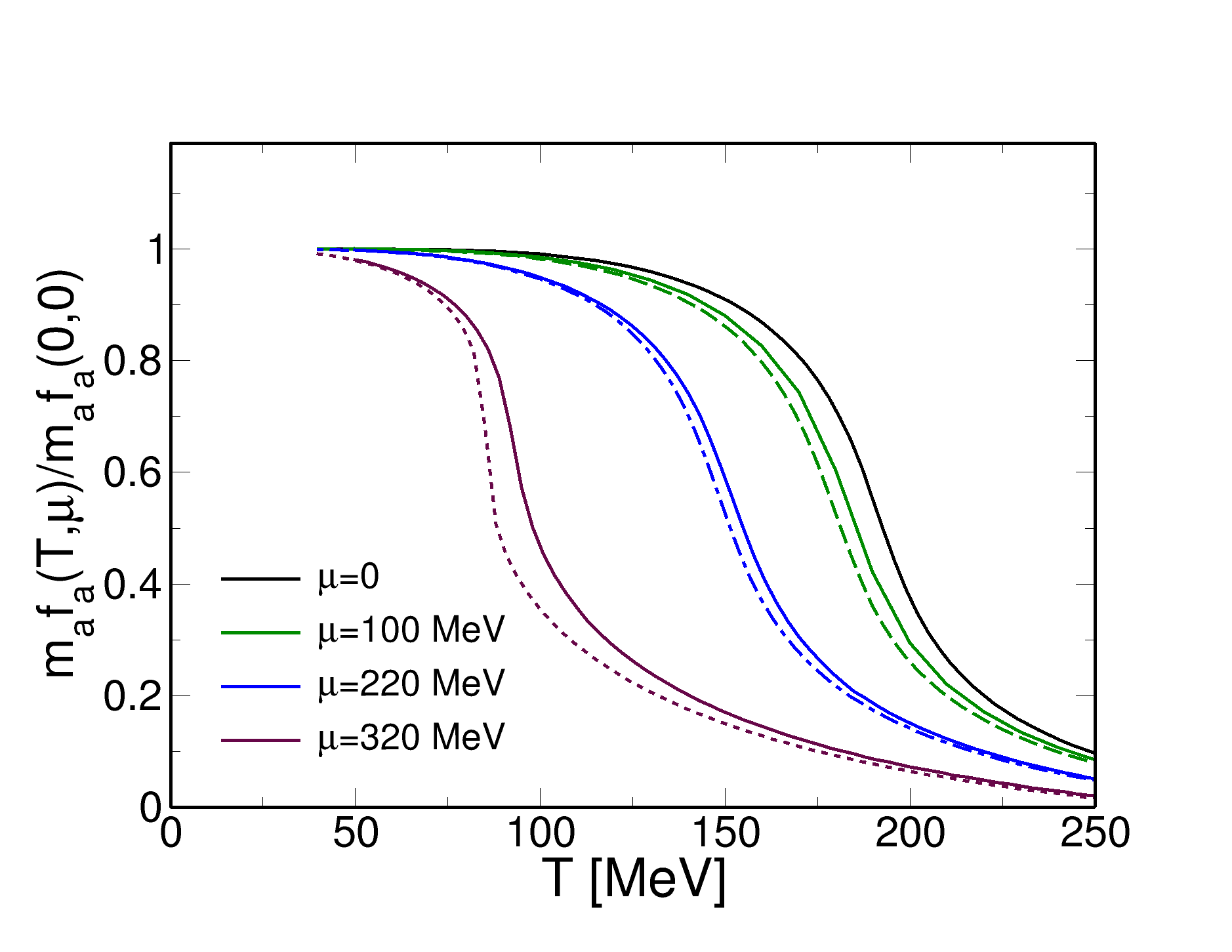
Figure 2: $m_{a}f_{a}$ versus $T$ for several values of $\mu$. Solid lines correspond to the calculations with electrical neutrality while dashed lines denote the results for $\mu_{e}=0$.

In Fig. 2 we plot $m_{a}f_{a}$, in units of the same quantity at $T=\mu=0$, namely

$$m_{a}f_{a}=6.38\times 10^{3}~{}\mathrm{MeV}^{2},$$ (19)

in agreement with previous estimates [53, 13]. In the figure we plot the results versus temperature, for several values of $\mu$. The solid lines denote the results obtained by taking electrical neutrality into account; for comparison, we show by the dashed lines the results obtained for $\mu_{e}=0$. We note that the decrease of $m_{a}$ with $T$ is slightly delayed by $\mu_{e}\neq 0$; besides this, we find no major differences between the cases with and without the neutrality condition.

From the numerical value of $m_{a}f_{a}$ in the vacuum we obtain the topological susceptibility, $\chi=m_{a}^{2}f_{a}^{2}$, which is $\chi\approx(79~{}\mathrm{MeV})^{4}$, again in agreement with previous works [53, 13]. We notice that in correspondence of the QCD crossover at finite temperature the axion mass drops significantly. Moreover, increasing $\mu$ results in a sharper drop of the axion mass, similarly to what happens to the chiral condensate. We conclude that the axion mass is very sensitive to the QCD phase transition.

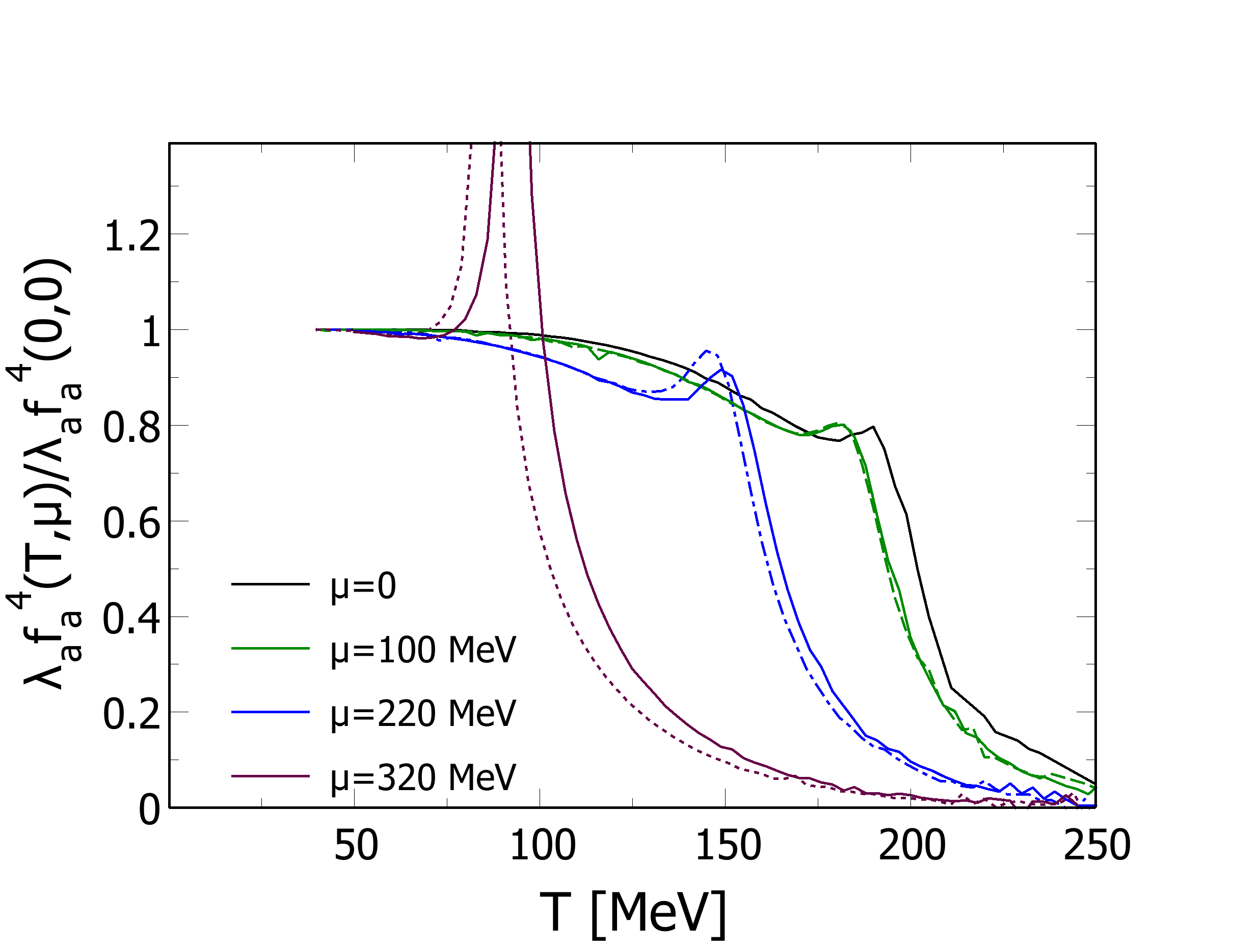
Figure 3: $\lambda_{a}f_{a}^{4}$ versus $T$ for several values of $\mu$. Solid lines correspond to the calculations with electrical neutrality while dashed lines denote the results for $\mu_{e}=0$.

In Fig. 3 we plot $\lambda_{a}f_{a}^{4}$ versus $T$ for several values of $\mu$. The solid lines correspond to the results obtained by imposing the electrical neutrality condition while the dashed lines denote those with $\mu_{e}=0$. At $T=\mu=0$ we find

$$\lambda_{a}f_{a}^{4}=-(55.63~{}\mathrm{MeV})^{4},$$ (20)

in agreement with previous calculations within the NJL model [53] and with $\chi$PT [13]. The fact that $\lambda_{a}<0$ means that the quartic interaction is attractive. We notice that in correspondence of the chiral crossover, the quartic coupling experiences a kink, in agreement with [57]; the kink becomes more pronounced when the crossover becomes sharper, namely when the critical endpoint is approached. Thus, despite the fact that $\lambda_{a}$ tends to become smaller with $T$, the chiral crossover enhances the axion self-coupling and this enhancement is very pronounced in proximity of the critical endpoint. We also note that imposing electrical neutrality does not qualitatively change the behavior of $\lambda_{a}$: the nonzero $\mu_{e}$ slightly pushes the chiral crossover to higher values of $T$; the peaks around the crossover are still present, and are quite substantial for large values of the quark chemical potential.

IV The axion potential and the domain walls

In this section we analyze the full axion potential (8), that we later use to analyze the axion domain walls and in particular to compute the surface tension. The potential $\Omega(\theta)$ in Eq. (8) is understood at the global minimum, namely computed at for the values of $\sigma$ and $\eta$ that minimize $\Omega$ for each value of $\theta$. In addition to that, since we consider electrically neutral matter, we fix $\mu_{e}$ in order to satisfy the condition (15) for $a\neq 0$.

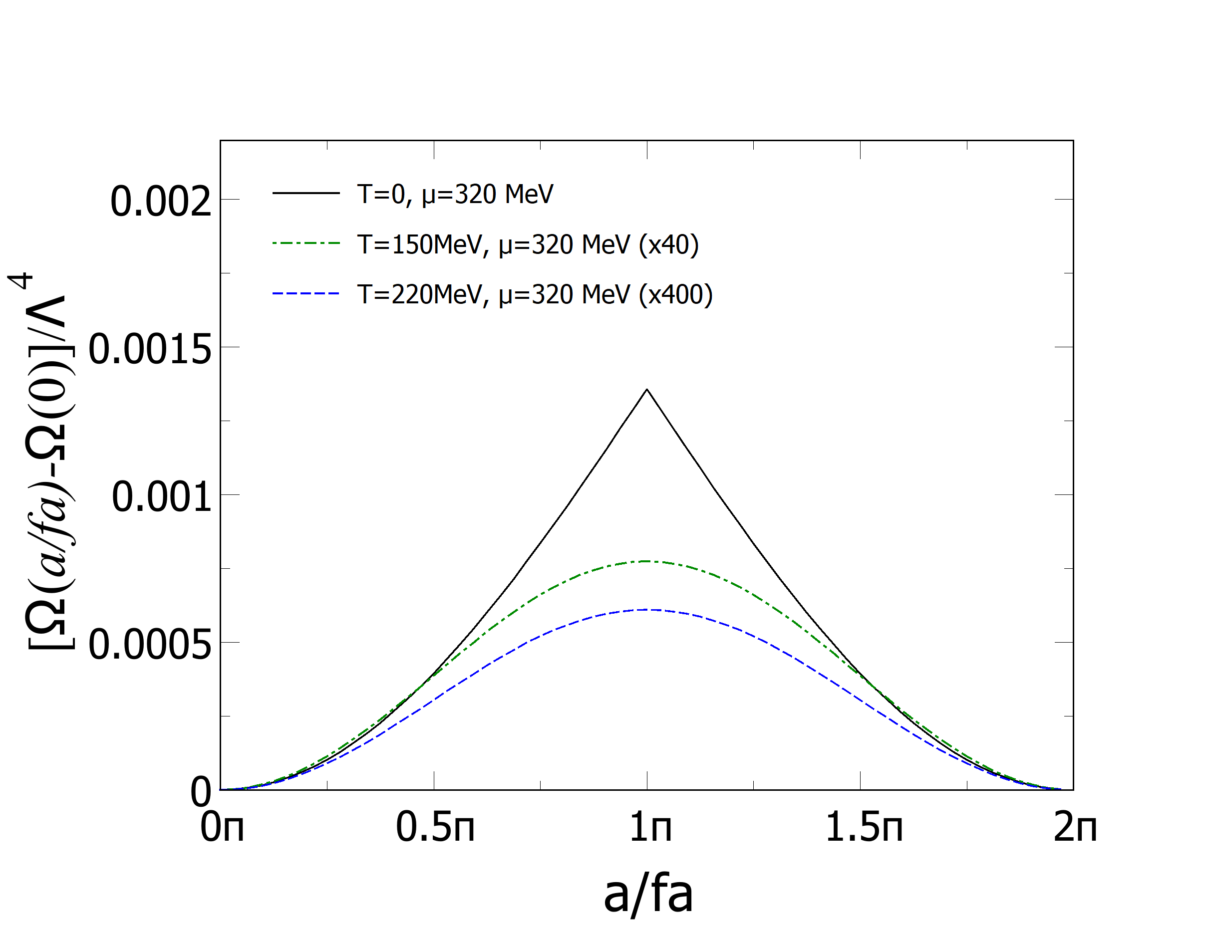
Figure 4: Axion potential at $\mu=320$ MeV, computed along the neutrality line. The potential is measured in units of the NJL cutoff $\Lambda$.

In Fig. 4 we plot the axion potential versus $a/f_{a}$ for several temperatures and for $\mu=320$ MeV; this has been computed along the neutrality line (15). The value at $a=0$ has been subtracted for later convenience, see Eq. (21). We note that increasing temperature results the lowering of the potential; this behavior is in qualitative agreement with previous results [53, 57]. We note that high chemical potential and temperature the barrier between the two degenerate vacua $a=0$ and $a/f_{a}=2\pi$ becomes several orders of magnitude smaller than that in the phase with chiral symmetry broken. Consequently, we expect that in the chiral restored phase the energy stored in solitons connecting the two vacua will be quite smaller than the one in the vacuum.

As a matter of fact, the potential shown in Fig. 4 gives rise to domain walls that interpolate between two successive vacua, because the potential is invariant under the discrete symmetry transformation $\theta\rightarrow\theta+2\pi n$ with $n\in Z$, while this symmetry is broken spontaneously by choosing one value of $a$, for example $a=0$. Derivation of the walls is quite standard and the details can be found textbooks, see for example [64, 65], hence here we report the main steps of the calculations only.

For the domain wall solution we consider the Lagrangian density

$$\mathcal{L}=\frac{1}{2}\partial^{\mu}a\partial_{\mu}a-V(a/f_{a}),$$ (21)

where we defined

$$V(x)=\Omega(x)-\Omega(0);$$ (22)

clearly, $V$ in the above equation depends on $\mu$ as well, but we suppress this dependence for the sake of notation. Incidentally, $V$ is the quantity shown in Fig. 4. Putting $a=\theta f_{a}$, the field equation that we get from $\mathcal{L}$ is

$$\partial_{\mu}\partial^{\mu}\theta+\frac{1}{f_{a}^{2}}\frac{\partial V(\theta)}{\partial\theta}=0.$$ (23)

The domain wall solution of Eq. (23) is a solitary wave,

$$\theta(x,t)=\theta(x-vt),$$ (24)

where $v$ denotes the propagation speed of the soliton. Putting $\xi=x-vt$ we can write Eq. (23) as

$$(1-v^{2})\theta_{\xi\xi}=\frac{1}{f_{a}^{2}}\frac{\partial V(\theta)}{\partial\theta}.$$ (25)

Multiplying both sides of (25) by $\theta_{\xi}$ and integrating, also noticing that we impose the boundary conditions $\theta\rightarrow 0$ and $\theta_{\xi}\rightarrow 0$ for $\xi\rightarrow\pm\infty$ we have

$$\frac{d\theta}{\sqrt{V(\theta)}}=\pm\sqrt{\frac{2}{f_{a}^{2}(1-v^{2})}}d\xi;$$ (26)

the $\pm$ sign correspond to the kink and antikink solutions respectively. The antikink connects $\theta=2\pi$ for $\xi\rightarrow-\infty$ to $\theta=0$ for $\xi\rightarrow+\infty$, while for the kink the two aforementioned limit values of $\theta$ are inverted. Equation (26) can be integrated by noticing that, for both the kink and the antikink, we can request that in the center of the soliton, $\xi=0$, we have $\theta(\xi)=\pi$. Then

$$\int_{\pi}^{\theta(\xi)}\frac{d\theta}{\sqrt{V(\theta)}}=\pm\xi\sqrt{\frac{2}{f_{a}^{2}(1-v^{2})}}.$$ (27)

The above equation defines implicitly the soliton $\theta(\xi)$.

In order to simplify the numerical evaluation of the integral on the left hand side of Eq. (27) we represent the potential by its Fourier cosine series,

$$V(\theta)=\frac{c_{0}}{2}+\sum_{n=1}^{N}c_{n}\cos(n\theta),$$ (28)

with

$$c_{n}=\frac{2}{\pi}\int_{0}^{\pi}d\theta~{}V(\theta)\cos(n\theta).$$ (29)

For the whole range of $(\mu,T)$ we consider in this study we find that $N=8$ in Eq. (28) is enough. Moreover, we find that for large $T/\mu$ the approximation $N=1$ works very well, with $c_{1}=-c_{0}/2\equiv-V_{0}$. For this particular case we have

$$V(\theta)=V_{0}(1-\cos\theta)=m_{a}^{2}f_{a}^{2}(1-\cos\theta).$$ (30)

For the potential (30) we can perform the integration in Eq. (27) easily to get

$$\theta_{\pm}(\xi)=4\arctan\exp\left(\pm\sqrt{\frac{m_{a}^{2}}{1-v^{2}}}\xi\right),$$ (31)

that, besides the rescaling brought by $m_{a}$, corresponds to the well-known soliton of the sine-Gordon equation, propagating along the $x-$direction with speed $c$.

In the following analysis we consider only solitons at rest: thus we put $c=0$ in Eq. (27) that implies $\xi=x$ and

$$\int_{\pi}^{\theta(x)}\frac{d\theta}{\sqrt{V(\theta)}}=\pm x\frac{\sqrt{2}}{f_{a}}.$$ (32)

For each $x$ the above equation allows us to compute the profile $\theta(x)$; the moving soliton is obtained from Eq. (32) by a Lorentz boost. Similarly, for the cosine potential (30) we have

$$\theta_{\pm}(x)=4\arctan\exp\left(\pm m_{a}x\right).$$ (33)

The above equation shows that the thickness of the wall is $\zeta=1/m_{a}$: consequently, from the results in Fig. 2 we conclude that chiral symmetry restoration (either at high temperature or large baryon density) results in the broadening of the axion walls.

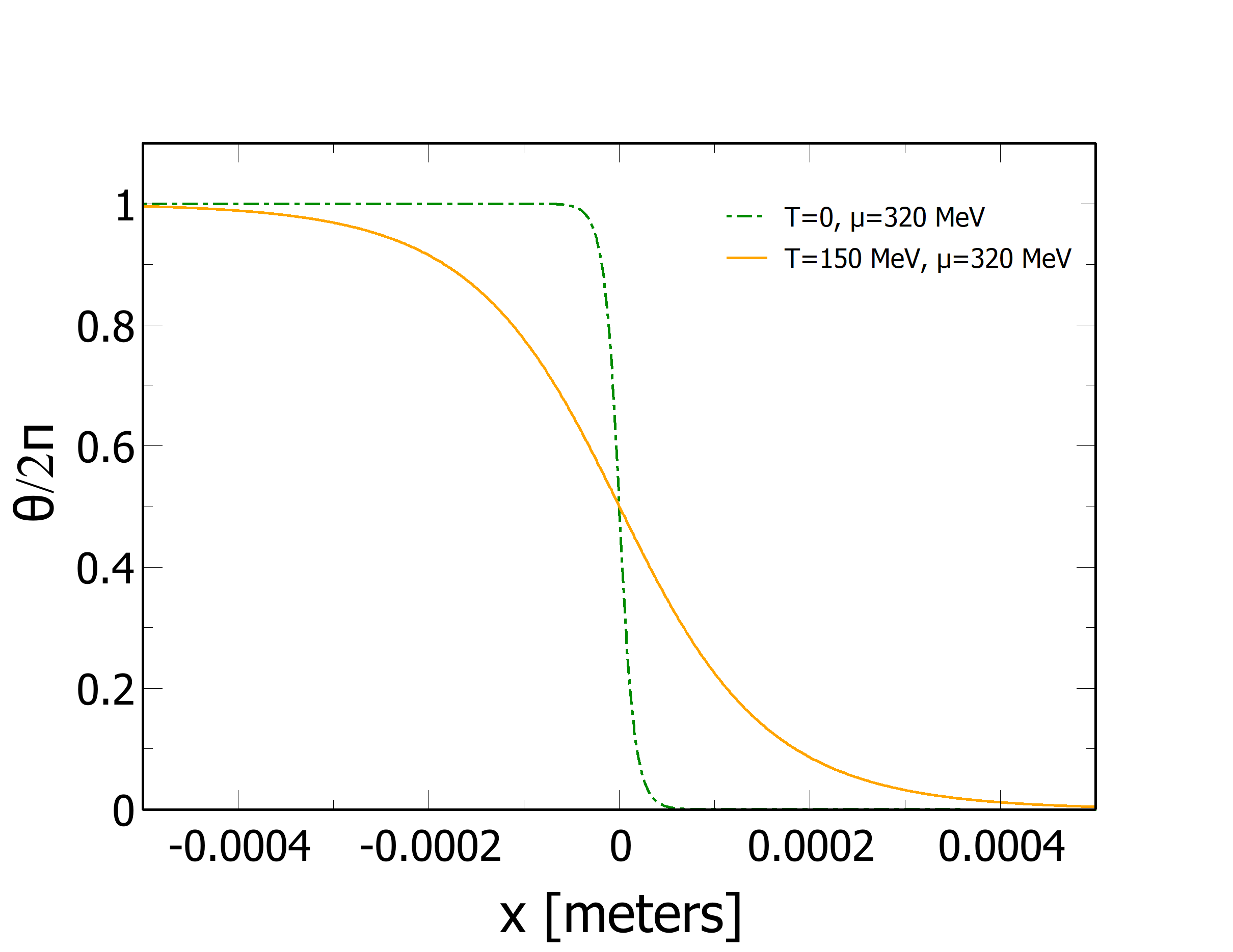
Figure 5: Axion walls, $\theta=a/f_{a}$, in the chiral broken phase (green dot-dashed line) and chiral symmetric phase (solid orange line).

In Fig. 5 we plot the axion wall profiles, $\theta=a/f_{a}$, in the chiral broken phase (green dot-dashed line) and in the chiral restored phase (orange solid line); we used $f_{a}=10^{9}$ GeV which is within the so-called classical axion window [66], see also [67] for more details, and $m_{a}$ was computed within the NJL model, see Fig. 2: we found $m_{a}\approx 6.4$ meV in the chiral symmetry broken phase and $m_{a}\approx 2.4$ meV in the chiral symmetry restored phase. The tiny value of the axion mass in the chiral restored phase explains why the spatial extension of the wall in this phase is of the order of $10^{-4}$ meters. The qualitative behavior of the walls is in agreement with the above discussion, namely restoring chiral symmetry results in the broadening of the walls. This implies the lowering of the surface tension of the wall, as we discuss later.

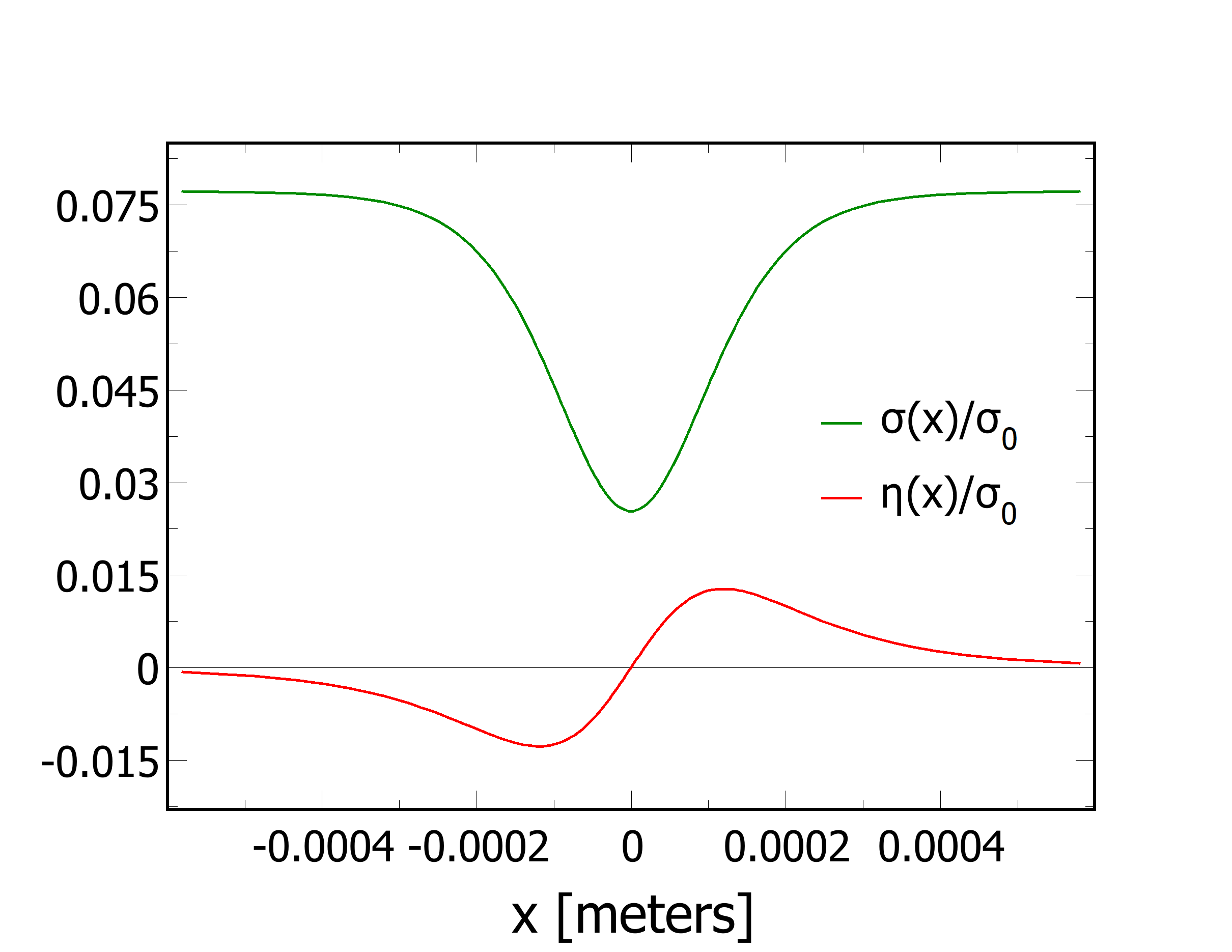
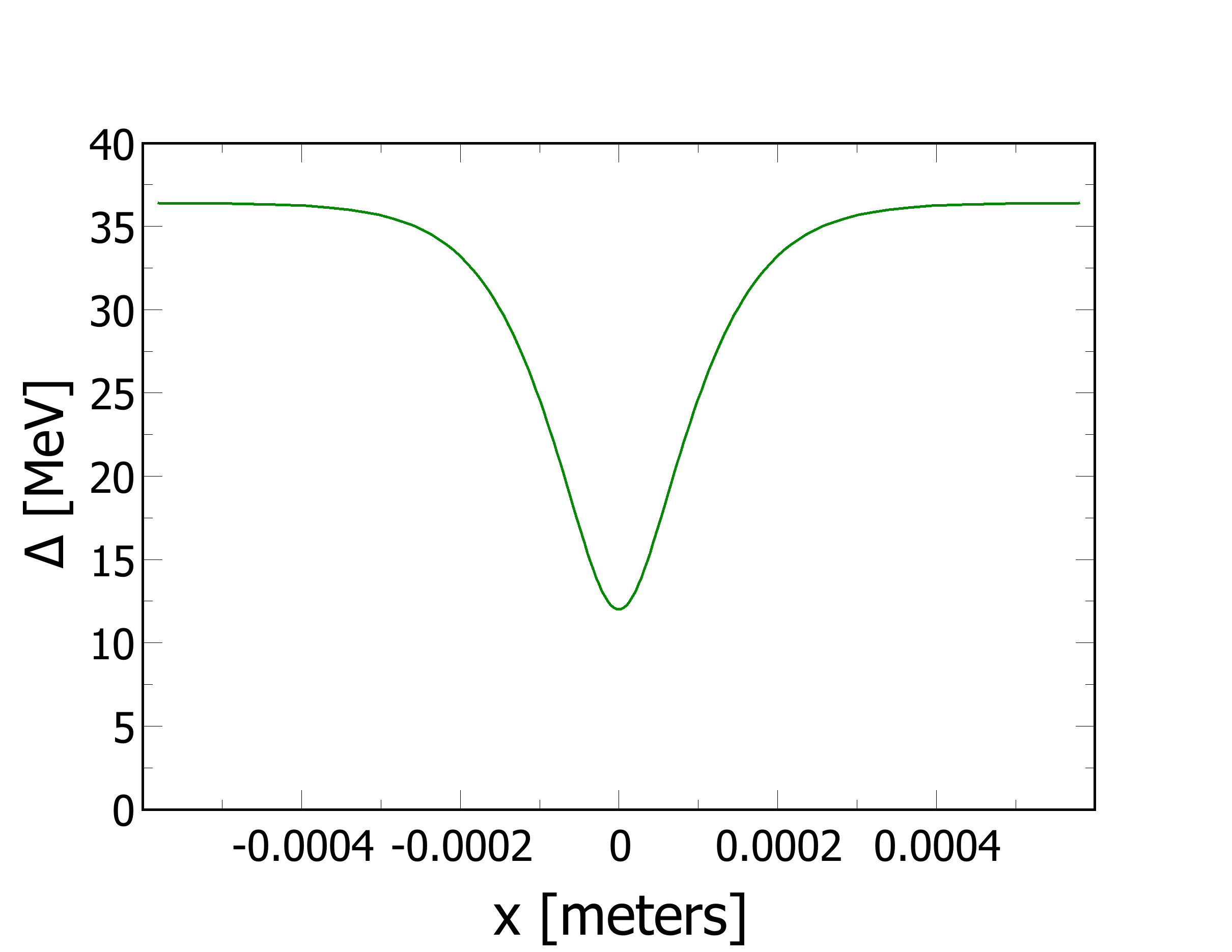
Figure 6: Condensaltes (upper panel) and fermion gap (lower panel) for the wall in cold and dense quark matter. We used $f_{a}=10^{9}$ GeV, while $m_{a}=1.48$meV resulting from the NJL model calculation. $\sigma_{0}$ corresponds to the condensate at $T=\mu=0$.

It is interesting to analyze the structure of the wall as we approach its center. In the upper panel of Fig. 6 we plot $\sigma$ and $\eta$ condensates along an axion wall in the cold and dense quark matter phase: calculations correspond to $\mu=400$ MeV and $T=10$ MeV. The condensates are measured in units of $\sigma_{0}=-2\times(241.5)^{3}$ MeV³ which corresponds to the condensate in the vacuum. In the lower panel of the same figure we plot the fermion gap $\Delta$ defined in Eq. (12). In this phase, the axion potential is well approximated by the cosine form (30). In order to compute the condensates we fixed $f_{a}=10^{9}$ GeV as before, then used the NJL model to compute $m_{a}\approx 1.48$ meV. We note that approaching the core of the wall, the $\eta$-condensate forms, signaling the spontaneous breaking of parity in that region. We also note that $\Delta$ decreases by a factor of $\approx 3$ near the core, meaning that quarks become lighter when they approach the inner region of the wall; for comparison, we checked that for the walls in the phase with chiral symmetry broken $\Delta$ decreases of a few percent only moving from the exterior part of the wall towards the core.

The energy per unit of transverse area, that is the surface tension $\kappa$, of the domain wall is defined as

$$\kappa=\int_{-\infty}^{+\infty}dx\left[\frac{1}{2}\left(\frac{da}{dx}\right)^{2}+V(a/f_{a})\right].$$ (34)

From the expression above it is easy to see that the wall gets most of its energy from the region where $|da/dx|$ and $V$ are larger, namely for $a/f_{\pi}=(2k+1)\pi$. Using $a=f_{a}\theta$ and Eq. (26) for $c=0$ we get

$$\kappa=2\sqrt{2}f_{a}\int_{0}^{\pi}d\theta\sqrt{V(\theta)},$$ (35)

which stands for both kink and antikink solutions. For the simple potential (30) this gives in particular

$$\kappa=8m_{a}f_{a}^{2}=\frac{8\chi}{m_{a}},$$ (36)

where $\chi$ denotes the topological susceptibility.

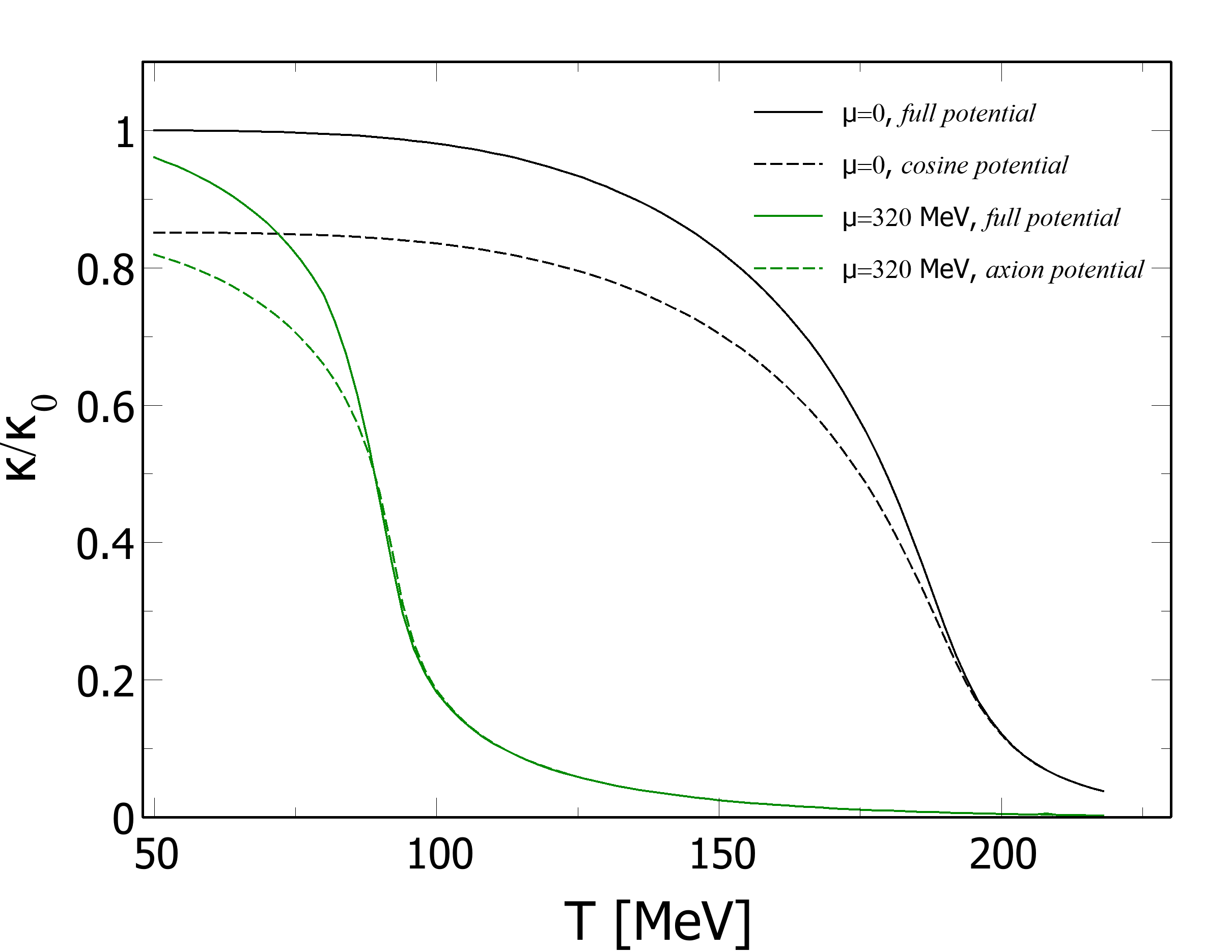
Figure 7: $\kappa$ versus temperature at $\mu=0$ (black lines) and $\mu=320$ MeV (green lines). Solid lines correspond to the results obtained with the full potential (22), while the dashed lines are the results obtained by virtue of the simplified cosine potential (30). $\kappa_{0}=1.9\times 10^{16}$ MeV³ is the surface tension computed at $T=\mu=0$.

In Fig. 7 we plot $\kappa$ versus temperature for $\mu=0$ (black lines) and $\mu=320$ MeV (green lines), computed along the neutrality line; solid lines correspond to the results obtained using the full axion potential (22), while the dashed lines are the results obtained by virtue of the simplified cosine potential (30). $\kappa$ is measured in units of the surface tension at $T=\mu=0$, which is $\kappa_{0}=1.9\times 10^{16}$ MeV³. We note that the QCD phase transition drastically affects the surface tension of the wall; particularly, in correspondence of chiral restoration $\kappa$ drops of about one order of magnitude for both values of $\mu$ shown.

We close this section with a comment on the possible abundance of axion walls in the cores of compact stars. From Eq. (36) we note that $\kappa$ can be a monstrous number in the vacuum; in the presence of dense quark matter, our calculations show that $\kappa$ can decrease of a few orders of magnitude at most, which still gives a gigantic surface tension. Therefore, one might conclude that forming the walls in quark matter is almost as prohibitive as forming the walls in the vacuum. However, this argument does not take into account of the background energy carried by quark matter itself: our conclusion is that in the thermodynamic limit, adding one wall to the bulk quark matter costs zero energy, therefore axion walls can form easily in presence of dense quark matter. To see this effect, for simplicity let us limit ourselves to the zero temperature case, which is a good approximation for the core of a compact star. Then, taking into account the domain wall, the energy density at $T=0$ is

$$\mathcal{E}=\frac{1}{2}\left(\frac{da}{dx}\right)^{2}+\Omega(\mu,a(x));$$ (37)

here $a(x)$ denotes the wall profile, so $\Omega(\mu,a(x))$ contains both the contribution of quark matter and that of the wall. We can add and subtract $\Omega(\mu,0)$ to the right hand side of the above equation, then subtract the irrelevant constant $\Omega(0,0)$, to get

$$\mathcal{E}=\mathcal{E}_{\mathrm{wall}}+\mathcal{E}_{\mathrm{quarks}},$$ (38)

where

$$\mathcal{E}_{\mathrm{wall}}=\frac{1}{2}\left(\frac{da}{dx}\right)^{2}+V[a(x)],$$ (39)

with $V$ is defined in Eq. (22), and

$$\mathcal{E}_{\mathrm{quarks}}=\Omega(\mu,0)-\Omega(0,0).$$ (40)

Thus, $\mathcal{E}_{\mathrm{wall}}$ corresponds to the energy density stored in the wall $a(x)$ at a given $\mu$, while $\mathcal{E}_{\mathrm{quarks}}$ is the free energy of bulk quark matter at the same $\mu$. In other words, adding the wall $a(x)$ to the bulk of quark matter requires an energy density $\mathcal{E}_{\mathrm{wall}}$. In the thermodynamic limit, $L\rightarrow\infty$, the energy of the wall grows $\sim L^{2}$; however, the energy of the background of quark matter grows $\sim\mu^{4}L^{3}$. Accordingly, the energy cost of adding one of these solitons to the bulk of quark matter is zero in this limit. We conclude that forming walls in bulk quark matter is easier than forming the walls in the vacuum, hence these walls might be abundant in the cores of compact stellar objects.

V Conclusions and outlook

We studied the QCD axion potential in dense quark matter. In particular, we analyzed the axion mass and self-coupling at finite temperature and/or baryon density. The interaction of axions to QCD matter, as well as the strong interaction, were modeled by a local NJL model. Our main goal was to study the effect of the chiral phase transition on the properties of the QCD axion. Interestingly, axions have been studied in astrophysical environments in the context of supernova explosions and protoneutron stars formation [68, 69]. Within this scenario, axions or axion like particles might be formed by means of the so called Primakoff process, which involves resonant production of neutral pseudoscalar mesons from the interaction of high-energy photons with atomic nuclei. The expected signals have been searched for in different data surveys, for instance in the Fermi-LAT data, where relevant the energy range covers 50 MeV to 500 GeV [70]. In addition, compact stars can potentially cool down by axion emissions that complement the standard neutrino and photon cooling [71, 72, 73, 74]. Keeping in mind potential applications of the results to the astrophysical compact objects, namely neutron stars or neutron stars mergers, we implemented bulk quark matter which is locally electrically neutral. We found that the chiral phase transition considerably affects the low energy properties of axions. In fact, the axion mass drops when chiral symmetry is restored. Moreover, the axion quartic self-coupling is enhanced when quark matter is close to the QCD critical endpoint.

We then computed the axion walls in dense quark matter, focusing on the surface tension of the solitons: to our knowledge, this is the first time that such a problem is considered. We noticed that the energy to form one of such walls in bulk quark matter has to be compared with the energy of the background matter: in the thermodynamic limit adding one wall to the bulk costs zero energy. As a consequence, adding walls to dense quark matter is not disfavored by energy arguments, and our conclusion is that it is likely that in bulk quark matter many axion walls form. The calculation of the full axion potential, in addition with the domain wall tension, shows that increasing $T$ and/or $\mu$ the potential well of the QCD axion becomes lower, thus making the transitions between the $\theta-$vacua easier.

Differently from calculations based on $\chi$PT, our work has at least two advantages. Firstly, it gives a result for the full axion potential, rather than an expansion around $a=0$. Moreover, it allows us to take into account the effect of the chiral phase transition on the axion potential, and these might have some impact, see for example the enhancement of $\lambda_{a}$ around the transition, or the lowering of $m_{a}$ in the chiral restored phase. These effects can not be obtained within $\chi$PT because in the latter the phase transition at finite temperature and/or chemical potential is missing.

As previously stated, this work paves the way to more complete model calculations as well as to interesting astrophysical applications. The results in Fig. 3 show that $\lambda_{a}$ is enhanced in proximity of the QCD critical endpoint: this implies that when quark matter is close to criticality, axions self-interaction is enhanced and this might favor the formation of self-bound axion droplets. While in our work this is purely speculative, this particular problem can be studied in detail and we aim at addressing it in the near future. Furthermore, the use of nonlocal covariant NJL models is very welcome, since these allow for a better comparison with lattice QCD data: studies of the coupling of axions to dense quark matter within nonlocal models are missing, so it is of a certain interest to extend the work we presented here to such models, possibly including a vector interaction. Moreover, it will be interesting to couple quarks to magnetic, and more generally to electromagnetic, fields, and study how this coupling affects the low energy properties of the axions. Even more, it is of a great interest to study the modifications of axions to the QCD equation of state at finite $T$ and $\mu$, having in mind applications to the structure of compact stars and neutron stars mergers. If axion walls can form inside compact stars, then they might affect the transport properties of nuclear and quark matter inside the stars themselves, because of the possible scatterings of nucleons and/or quarks on the walls. We leave these interesting problems to near future works.

- [1] R. J. Crewther, P. Di Vecchia, G. Veneziano, and E. Witten. Phys. Lett. B, 88, 123 (1979). doi:10.1016/0370-2693(79)90128-X
- [2] C. A. Baker, D. D. Doyle, P. Geltenbort, K. Green, M. G. D. van der Grinten, P. G. Harris, P. Iaydjiev, S. N. Ivanov, D. J. R. May and J. M. Pendlebury, et al. Phys. Rev. Lett. 97, 131801 (2006) doi:10.1103/PhysRevLett.97.131801 [arXiv:hep-ex/0602020 [hep-ex]].
- [3] W. C. Griffith, M. D. Swallows, T. H. Loftus, M. V. Romalis, B. R. Heckel and E. N. Fortson, Phys. Rev. Lett. 102, 101601 (2009) doi:10.1103/PhysRevLett.102.101601 [arXiv:0901.2328 [physics.atom-ph]].
- [4] R. H. Parker, M. R. Dietrich, M. R. Kalita, N. D. Lemke, K. G. Bailey, M. Bishof, J. P. Greene, R. J. Holt, W. Korsch and Z. T. Lu, et al. Phys. Rev. Lett. 114, no.23, 233002 (2015) doi:10.1103/PhysRevLett.114.233002 [arXiv:1504.07477 [nucl-ex]].
- [5] B. Graner, Y. Chen, E. G. Lindahl and B. R. Heckel, Phys. Rev. Lett. 116, no.16, 161601 (2016) [erratum: Phys. Rev. Lett. 119, no.11, 119901 (2017)] doi:10.1103/PhysRevLett.116.161601 [arXiv:1601.04339 [physics.atom-ph]].
- [6] N. Yamanaka, T. Yamada, E. Hiyama and Y. Funaki, Phys. Rev. C 95, no.6, 065503 (2017) doi:10.1103/PhysRevC.95.065503 [arXiv:1603.03136 [nucl-th]].
- [7] F. K. Guo, R. Horsley, U. G. Meissner, Y. Nakamura, H. Perlt, P. E. L. Rakow, G. Schierholz, A. Schiller and J. M. Zanotti, Phys. Rev. Lett. 115, no.6, 062001 (2015) doi:10.1103/PhysRevLett.115.062001 [arXiv:1502.02295 [hep-lat]].
- [8] T. Bhattacharya, V. Cirigliano, R. Gupta, H. W. Lin and B. Yoon, Phys. Rev. Lett. 115, no.21, 212002 (2015) doi:10.1103/PhysRevLett.115.212002 [arXiv:1506.04196 [hep-lat]].
- [9] R. D. Peccei and H. R. Quinn, Phys. Rev. Lett. 38, 1440-1443 (1977) doi:10.1103/PhysRevLett.38.1440
- [10] R. D. Peccei and H. R. Quinn, Phys. Rev. D 16, 1791-1797 (1977) doi:10.1103/PhysRevD.16.1791
- [11] S. Weinberg, Phys. Rev. Lett. 40, 223-226 (1978) doi:10.1103/PhysRevLett.40.223
- [12] F. Wilczek, Phys. Rev. Lett. 40, 279-282 (1978) doi:10.1103/PhysRevLett.40.279
- [13] G. Grilli di Cortona, E. Hardy, J. Pardo Vega and G. Villadoro, JHEP 01, 034 (2016) doi:10.1007/JHEP01(2016)034 [arXiv:1511.02867 [hep-ph]].
- [14] J. E. Kim and G. Carosi, Rev. Mod. Phys. 82, 557-602 (2010) [erratum: Rev. Mod. Phys. 91, no.4, 049902 (2019)] doi:10.1103/RevModPhys.82.557 [arXiv:0807.3125 [hep-ph]].
- [15] D. A. Easson, I. Sawicki and A. Vikman, JCAP 11, 021 (2011) doi:10.1088/1475-7516/2011/11/021 [arXiv:1109.1047 [hep-th]].
- [16] E. Berkowitz, M. I. Buchoff and E. Rinaldi, Phys. Rev. D 92, no.3, 034507 (2015) doi:10.1103/PhysRevD.92.034507 [arXiv:1505.07455 [hep-ph]].
- [17] L. D. Duffy and K. van Bibber, New J. Phys. 11, 105008 (2009) doi:10.1088/1367-2630/11/10/105008 [arXiv:0904.3346 [hep-ph]].
- [18] M. S. Turner and F. Wilczek, Phys. Rev. Lett. 66, 5-8 (1991) doi:10.1103/PhysRevLett.66.5
- [19] L. Visinelli and P. Gondolo, Phys. Rev. D 80, 035024 (2009) doi:10.1103/PhysRevD.80.035024 [arXiv:0903.4377 [astro-ph.CO]].
- [20] I. I. Tkachev, Phys. Lett. B 261, 289-293 (1991) doi:10.1016/0370-2693(91)90330-S
- [21] E. W. Kolb and I. I. Tkachev, Phys. Rev. Lett. 71, 3051-3054 (1993) doi:10.1103/PhysRevLett.71.3051 [arXiv:hep-ph/9303313 [hep-ph]].
- [22] P. H. Chavanis, Phys. Rev. D 84, 043531 (2011) doi:10.1103/PhysRevD.84.043531 [arXiv:1103.2050 [astro-ph.CO]].
- [23] F. S. Guzman and L. A. Urena-Lopez, Astrophys. J. 645, 814-819 (2006) doi:10.1086/504508 [arXiv:astro-ph/0603613 [astro-ph]].
- [24] J. Barranco and A. Bernal, Phys. Rev. D 83, 043525 (2011) doi:10.1103/PhysRevD.83.043525 [arXiv:1001.1769 [astro-ph.CO]].
- [25] E. Braaten, A. Mohapatra and H. Zhang, Phys. Rev. Lett. 117, no.12, 121801 (2016) doi:10.1103/PhysRevLett.117.121801 [arXiv:1512.00108 [hep-ph]].
- [26] S. Davidson and T. Schwetz, Phys. Rev. D 93, no.12, 123509 (2016) doi:10.1103/PhysRevD.93.123509 [arXiv:1603.04249 [astro-ph.CO]].
- [27] J. Eby, M. Leembruggen, P. Suranyi and L. C. R. Wijewardhana, JHEP 12, 066 (2016) doi:10.1007/JHEP12(2016)066 [arXiv:1608.06911 [astro-ph.CO]].
- [28] T. Helfer, D. Marsh, K. Clough, M. Fairbairn, E. Lim, and R. Becerril, J. Cosmol. Astropart. Phys. 03 (2017) 055 doi:10.1088/1475-7516/2017/03/055 [arXiv:1609.04724 [astro-ph.CO]].
- [29] D. G. Levkov, A. G. Panin and I. I. Tkachev, Phys. Rev. Lett. 118, no.1, 011301 (2017) doi:10.1103/PhysRevLett.118.011301 [arXiv:1609.03611 [astro-ph.CO]].
- [30] J. Eby, M. Leembruggen, P. Suranyi and L. C. R. Wijewardhana, JHEP 06, 014 (2017) doi:10.1007/JHEP06(2017)014 [arXiv:1702.05504 [hep-ph]].
- [31] L. Visinelli, S. Baum, J. Redondo, K. Freese and F. Wilczek, Phys. Lett. B 777, 64-72 (2018) doi:10.1016/j.physletb.2017.12.010 [arXiv:1710.08910 [astro-ph.CO]].
- [32] P. H. Chavanis, Phys. Rev. D 94, no.8, 083007 (2016) doi:10.1103/PhysRevD.94.083007 [arXiv:1604.05904 [astro-ph.CO]].
- [33] E. Cotner, Phys. Rev. D 94, no.6, 063503 (2016) doi:10.1103/PhysRevD.94.063503 [arXiv:1608.00547 [astro-ph.CO]].
- [34] Y. Bai, V. Barger and J. Berger, JHEP 12, 127 (2016) doi:10.1007/JHEP12(2016)127 [arXiv:1612.00438 [hep-ph]].
- [35] P. Sikivie and Q. Yang, Phys. Rev. Lett. 103, 111301 (2009) doi:10.1103/PhysRevLett.103.111301 [arXiv:0901.1106 [hep-ph]].
- [36] P. H. Chavanis, Phys. Rev. D 98, no.2, 023009 (2018) doi:10.1103/PhysRevD.98.023009 [arXiv:1710.06268 [gr-qc]].
- [37] R. Brower, S. Chandrasekharan, J. W. Negele and U. J. Wiese, Phys. Lett. B 560, 64-74 (2003) doi:10.1016/S0370-2693(03)00369-1 [arXiv:hep-lat/0302005 [hep-lat]].
- [38] Y. Y. Mao et al. [TWQCD], Phys. Rev. D 80, 034502 (2009) doi:10.1103/PhysRevD.80.034502 [arXiv:0903.2146 [hep-lat]].
- [39] S. Aoki and H. Fukaya, Phys. Rev. D 81, 034022 (2010) doi:10.1103/PhysRevD.81.034022 [arXiv:0906.4852 [hep-lat]].
- [40] V. Bernard, S. Descotes-Genon and G. Toucas, JHEP 12, 080 (2012) doi:10.1007/JHEP12(2012)080 [arXiv:1209.4367 [hep-lat]].
- [41] V. Bernard, S. Descotes-Genon and G. Toucas, JHEP 06, 051 (2012) doi:10.1007/JHEP06(2012)051 [arXiv:1203.0508 [hep-ph]].
- [42] M. A. Metlitski and A. R. Zhitnitsky, Phys. Lett. B 633, 721-728 (2006) doi:10.1016/j.physletb.2006.01.001 [arXiv:hep-ph/0510162 [hep-ph]].
- [43] S. Borsanyi, Z. Fodor, J. Guenther, K. H. Kampert, S. D. Katz, T. Kawanai, T. G. Kovacs, S. W. Mages, A. Pasztor and F. Pittler, et al. Nature 539, no.7627, 69-71 (2016) doi:10.1038/nature20115 [arXiv:1606.07494 [hep-lat]].
- [44] S. Aoki et al. [JLQCD], EPJ Web Conf. 175, 04008 (2018) doi:10.1051/epjconf/201817504008 [arXiv:1712.05541 [hep-lat]].
- [45] C. Bonati, M. D’Elia, M. Mariti, G. Martinelli, M. Mesiti, F. Negro, F. Sanfilippo and G. Villadoro, JHEP 03, 155 (2016) doi:10.1007/JHEP03(2016)155 [arXiv:1512.06746 [hep-lat]].
- [46] Y. Nambu and G. Jona-Lasinio, Phys. Rev. 124, 246-254 (1961) doi:10.1103/PhysRev.124.246
- [47] Y. Nambu and G. Jona-Lasinio, Phys. Rev. 122, 345-358 (1961) doi:10.1103/PhysRev.122.345
- [48] M. Buballa, Phys. Rept. 407, 205-376 (2005) doi:10.1016/j.physrep.2004.11.004 [arXiv:hep-ph/0402234 [hep-ph]].
- [49] T. Hatsuda and T. Kunihiro, Phys. Rept. 247, 221-367 (1994) doi:10.1016/0370-1573(94)90022-1 [arXiv:hep-ph/9401310 [hep-ph]].
- [50] S. P. Klevansky, Rev. Mod. Phys. 64, 649-708 (1992) doi:10.1103/RevModPhys.64.649
- [51] Y. Nambu and G. Jona-Lasinio, Phys. Rev. 122, 345-358 (1961) doi:10.1103/PhysRev.122.345
- [52] Y. Nambu and G. Jona-Lasinio, Phys. Rev. 124, 246-254 (1961) doi:10.1103/PhysRev.124.246
- [53] Z. Y. Lu and M. Ruggieri, Phys. Rev. D 100, no.1, 014013 (2019) doi:10.1103/PhysRevD.100.014013 [arXiv:1811.05102 [hep-ph]].
- [54] B. S. Lopes, R. L. S. Farias, V. Dexheimer, A. Bandyopadhyay and R. O. Ramos, Phys. Rev. D 106 (2022) no.12, L121301 doi:10.1103/PhysRevD.106.L121301 [arXiv:2206.01631 [hep-ph]].
- [55] A. Bandyopadhyay, R. L. S. Farias, B. S. Lopes and R. O. Ramos, Phys. Rev. D 100 (2019) no.7, 076021 doi:10.1103/PhysRevD.100.076021 [arXiv:1906.09250 [hep-ph]].
- [56] A. Das, H. Mishra and R. K. Mohapatra, Phys. Rev. D 103 (2021) no.7, 074003 doi:10.1103/PhysRevD.103.074003 [arXiv:2006.15727 [hep-ph]].
- [57] R. K. Mohapatra, A. Abhishek, A. Das and H. Mishra, Springer Proc. Phys. 277, 455-458 (2022) doi:10.1007/978-981-19-2354-8_83
- [58] P. Sikivie, Phys. Rev. Lett. 48, 1156-1159 (1982) doi:10.1103/PhysRevLett.48.1156
- [59] G. Gabadadze and M. A. Shifman, Phys. Rev. D 62, 114003 (2000) doi:10.1103/PhysRevD.62.114003 [arXiv:hep-ph/0007345 [hep-ph]].
- [60] S. B. Ruester, V. Werth, M. Buballa, I. A. Shovkovy and D. H. Rischke, Phys. Rev. D 72, 034004 (2005) doi:10.1103/PhysRevD.72.034004 [arXiv:hep-ph/0503184 [hep-ph]].
- [61] D. Blaschke, S. Fredriksson, H. Grigorian, A. M. Oztas and F. Sandin, Phys. Rev. D 72, 065020 (2005) doi:10.1103/PhysRevD.72.065020 [arXiv:hep-ph/0503194 [hep-ph]].
- [62] G. ’t Hooft, Phys. Rev. D 14, 3432-3450 (1976) [erratum: Phys. Rev. D 18, 2199 (1978)] doi:10.1103/PhysRevD.14.3432
- [63] G. ’t Hooft, Phys. Rept. 142, 357-387 (1986) doi:10.1016/0370-1573(86)90117-1
- [64] Y. Nagashima, Beyond the standard model of elementary particle physics, Wiley-VCH, 2014, ISBN 978-3-527-41177-1, 978-3-527-66505-1
- [65] M. Shifman, Advanced Topics in Quantum Field Theory, Cambridge University Press, 2022, ISBN 978-1-108-88591-1, 978-1-108-84042-2 doi:10.1017/9781108885911
- [66] F. Takahashi, W. Yin and A. H. Guth, Phys. Rev. D 98, no.1, 015042 (2018) doi:10.1103/PhysRevD.98.015042 [arXiv:1805.08763 [hep-ph]].
- [67] R. L. Workman et al. [Particle Data Group], PTEP 2022 (2022), 083C01 doi:10.1093/ptep/ptac097
- [68] G. Lucente, P. Carenza, T. Fischer, M. Giannotti and A. Mirizzi, JCAP 12, 008 (2020) doi:10.1088/1475-7516/2020/12/008 [arXiv:2008.04918 [hep-ph]].
- [69] T. Fischer, P. Carenza, B. Fore, M. Giannotti, A. Mirizzi and S. Reddy, Phys. Rev. D 104, no.10, 103012 (2021) doi:10.1103/PhysRevD.104.103012 [arXiv:2108.13726 [hep-ph]].
- [70] F. Calore, P. Carenza, C. Eckner, T. Fischer, M. Giannotti, J. Jaeckel, K. Kotake, T. Kuroda, A. Mirizzi and F. Sivo, Phys. Rev. D 105, no.6, 063028 (2022) doi:10.1103/PhysRevD.105.063028 [arXiv:2110.03679 [astro-ph.HE]].
- [71] L. B. Leinson, JCAP 08, 031 (2014) doi:10.1088/1475-7516/2014/08/031 [arXiv:1405.6873 [hep-ph]].
- [72] A. Sedrakian, Phys. Rev. D 93, no.6, 065044 (2016) doi:10.1103/PhysRevD.93.065044 [arXiv:1512.07828 [astro-ph.HE]].
- [73] A. Sedrakian, Phys. Rev. D 99, no.4, 043011 (2019) doi:10.1103/PhysRevD.99.043011 [arXiv:1810.00190 [astro-ph.HE]].
- [74] M. Buschmann, C. Dessert, J. W. Foster, A. J. Long and B. R. Safdi, Phys. Rev. Lett. 128, no.9, 091102 (2022) doi:10.1103/PhysRevLett.128.091102 [arXiv:2111.09892 [hep-ph]].