Mathematical modeling of trend cycle: Fad, Fashion and Classic

Abstract.

In this work, we suggest a system of differential equations that quantitatively models the formulation and evolution of a trend cycle through the consideration of underlying dynamics between the trend participants. Our model captures the five stages of a trend cycle, namely, the onset, rise, peak, decline, and obsolescence. It also provides a unified mathematical criterion/condition to characterize the fad, fashion and classic. We prove that the solution of our model can capture various trend cycles. Numerical simulations are provided to show the expressive power of our model.

1. Introduction

People have a tendency to follow or mimic others in a human society, which can be described as a fashion or trend. A trend arises in many markets: in a financial market (Tulip mania [31], Bitcoin frenzy [21], etc.), a clothing industry (leggings in fast fashion brands [6]), a food industry (Organic food product trend [27]), an entertainment industry (Hallyu [17]), and in an electronic device market (Smartphones becoming fashion ). Such trends, upto some inevitable oversimplification, go through a cycle consisting of onset, rise, peak, decline, and obsolescence. A trend emerges as a small number of early adopters take the trend (onset). More people start to join the trend (rise). After the number of adopters reaches its peak (peak), some begin to leave the trend losing their interest in it (decline). Eventually, the trend loses its influencing power and is finally forgotten (obsolescence). These stages constitute a trend cycle. (See Figure 1 from [14])

Figure 1. Classification of a trend: Fad, Fashion, and Classic (Source: Susan Kaiser, The Social Psychology of Clothing[14])

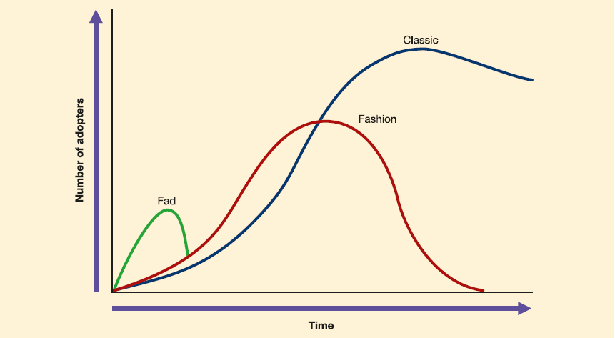
Such trend cycles are often categorized into Fad, Fashion and Classic. Fad usually refers to a short-lived trend: it gains large popularity over a short period of time, and disappears quickly. A trend that lasts longer and is taken by a larger population is called Fashion. Classic is a style that has firmly settled in a society or the market. It persists over a much more extended time period. Usually, it enjoys more royalty from customers and is less volatile. But the precise definitions of Fad, Fashion and Classic are not available in the literature (e.g.[4, 12, 32]). Besides the facts that Fad lasts shorter than Fashion, and Classic lasts longer than Fashion, there exists no clear feature that plays as a dividing pole between these three different cycles. For example, it may depend on the business. The usual lifespan of Fad (e.g. Squid Game, Viral video clips on YouTube or TikTok, and Psy’s popular song Gangnam Style) in an entertainment business can be much shorter than that of Fad in the fashion industry or electric device industry (e.g. Blackberry and portable media player). Moreover, Fashion may arise as a renovated form of an existing fashion style (e.g. various styles of jeans). Some products of brands such as Coca-Cola, Louis Vuitton, and Chanel are considered as examples of classical items.

The purpose of this work is twofold. First, we provide a dynamic modeling of the trend cycle. We introduce a system of differential equations that, through the consideration of underlying dynamics between the market participants, explains the formation of the trend cycle. We adopt a simple picture that a society is divided into three groups: people who have not joined a particular trend yet, people who have adopted the trend, and people who have left the trend. We then recognize the analogy between the infection/recovery processes in an epidemic spread, and the adoption/rejection processes in a trend cycle to derive dynamic laws between the three groups.

Secondly, based on this model, we provide a mathematically rigorous criterion to characterize Fad, Fashion, and Classic. As mentioned above, a trend cycle is dubbed fad, fashion, and classic based on the volatility of the trend. But a clear guideline to characterize them does not exist. In this regard, we observe that the fad, fashion, and classic can be divided by the way how participants leave the trend. As we can see in Figure 1, this is reflected in the steepness of the slope in the trend cycle at the stages of decline and obsolescence. This, in turn, can be realized in our differential model by a suitable choice of rejection rates and parameters (see Sec. 2). Our description of a trend cycle provides a rigorous way to characterize these three different types of trends in a precise way. We define a fad as a cycle that extincts in a finite time, leading to hard landing of the curve in a finite time. Classic can be defined by the curve declining at most polynomial order in the long run. Fashion is defined as a trend cycle that lies between them. The seasonal revival of a fashion trend can also be captured. Our trend cycle model provides a unified framework to understand various different types of trends: a fashion trend, a literature style, a commodity’s popularity, a cultural frenzy in music and movie, a speculative behavior in a cryptocurrency market.

Studies on a trend cycle involve numerous topics such as marketing, legal issues, consumer behavior, technology, media, historical analysis, cultural study, etc. An exhaustive review on such a broad topic is not plausible. We focus on the literature that is directly relevant to ours. In [26], a trend cycle model is developed to study how a new design is created, and its popularity eventually falls over time as it spreads across the population. The advent of various social media significantly impacts the fashion trend these days. In [24], the author examines the relationship between social media and fashion. [16] investigates the impacts of social media marketing on customers’ intimacy and trust in the luxury brand. On the other hand, a recent study in [8] shows that consumers’ emotion becomes a key factor in determining the fashion trend. In a seminal work [12], Hemphill and Suk described the evolution of a fashion trend by combining the effect of flocking and differentiation and investigated various legal issues in the fashion industry based on such an observation. The study on the spread of a fashion trend between social classes has been studied which can be categorized roughly into the following three types: trickle-down theory (spread of a fashion from upper to lower class), trickle-up theory (spread of a fashion from lower to upper class), and trickle-across theory (horizontal movement of fashion) [29, 12, 23]. See [9, 10, 14, 18, 12] and references therein for an overview of various topics in fashion.

As mentioned above, our model has analogy with the epidemic spread model (e.g. susceptible-infected-recovered (SIR) type models). Therefore, a brief review of SIR-type models is in order. Since the inception of the model in [15], the SIR model has been widely used for quantitative modeling of epidemics [3, 11, 19, 28]. The SIR model is also successfully employed to study the recent Covid-19 pandemic to understand the spread mechanism and forecast the possible progress of the pandemic [13, 20, 1, 25].

The paper is organized as follows: in Sec. 2, we derive a system of differential equations that describes the dynamics of a trend cycle. In Sec. 3, we verify that the solution of our model satisfies the desired decaying properties. In Sec. 4, we carry out various numerical experiments to justify our model. In Sec 5, we draw conclusions of the paper.

2. Dynamic modelling of trend cycle

We derive a system of differential equations to describe a trend cycle. For this, we introduce three variables that correspond to the number of potential adopters of a trend, the number of people who adopted the trend, and the number of people who left the trend. We then derive a dynamic law between these three groups by observing how they adopt a trend and how they reject it.

First, we define the three dynamic variables:

• $S(t)$: the number of potential adopters of a trend at time $t$,

• $I(t)$: the number of people who have adopted the trend at time $t$,

• $R(t)$: the number of people who have left the trends at time $t$.

Note that, by definition, any reasonable model must satisfy

(2.1) $$N=S(t)+I(t)+R(t)\quad t\geq 0,$$

where $N$ is the number of individuals in a society. We now consider how these compartments in the trend interact through the adoption and rejection.

$\bullet$ Equation for the evolution of $I$: We start with the derivation of dynamic equation for $I$. The equations for other variables follow almost automatically once the equation for $I$ is determined. For this, we consider two factors below: the adoption, and rejection of a trend.

Trend Adoption: Our main assumption is that the adoption rate of a new trend depends on how often people in a society are exposed to the trend. Here, we assume such exposure is expressed in the following multiplicative law:

(2.2) $$\alpha(t)\frac{I(t)}{N}S(t)$$

for a suitable adoption rate $\alpha$ at each time $t$. It remains to determine $\alpha(t)$. For this, we make the following reasonable assumption on the adoption rate: 1) as the ratio of people adopting the trend increases, people get more interested in the trend (that is, $\alpha$ is a monotonic function of $I/N$); 2) As the number of people adopting the trend starts to decrease, people get less interested in the trend. A suitable adoption rate satisfying these assumptions is a sigmoid function:

(2.3) $$\begin{split}\alpha(t):=\alpha\left(\frac{I(t)}{N}\right)=\frac{m_{1}}{1+\exp\left(-m_{2}\left(\frac{I(t)}{N}-\ell_{\alpha}\right)\right)},\end{split}$$

where $m_{1}>0$ and $m_{2}>0$ describe the intensity of the adoption and the sharpness of the transition, and $\ell_{\alpha}$ is the adoption delay.

Trend Rejection: To describe how people reject a trend, we employ the following simple expression, which says that the number of people leaving the trend is proportional to $I$:

$$\beta(t)I(t).$$

Our main assumption in choosing the appropriate $\beta(t)$ is that people barely leave the trend when the trend is rising, but start to leave the trend after the trend hits the peak. It is how quickly people lose their interest after the number of trend-followers gets saturated. For this, we let $t=t_{*}$ to be the first time on which $I$ takes the maximum value, which will be called the transition:

$$t_{*}:=\inf\left\{t>0\hskip 0.56905pt|\hskip 0.56905pt\,I^{\prime}(t)=0.\right\}$$

Then, we define the rejection rate as follows: $(p\in\mathbb{R})$

(2.6) $$\beta(t):=\beta\left(\frac{I(t)}{N}\right)=\left\{\begin{array}[]{ll}\frac{m_{3}}{1+\exp\left(-m_{4}\left(\frac{I(t)}{N}-\ell_{\beta}\right)\right)}&~{}(t\leq t_{*}),\\ C_{*}\left(\frac{I(t)}{N}\right)^{p}&~{}(t>t_{*}),\end{array}\right.$$

where $C_{*}$ denotes

$$C_{*}=\beta(t_{*})\left(\frac{I(t_{*})}{N}\right)^{-p}.$$

We note that $m_{3},m_{4}>0$ describe the intensity of rejection and the sharpness of the transition, and $\ell_{\beta}\in\mathbb{R}$ is the delay in rejection. Note also that there are cases when $I$ decreases from $t=0$. We can set $t_{*}$ to be infinity in this case.

The intuition behind this choice of $\beta$ is as follows: Since $I$ decreases after $t=t_{*}$, the case $p\geq 0$ corresponds to the case when the rate of rejection is slowing down leading to the tail that lasts forever. On the other hand, $p<0$ corresponds to the case when the rate of rejection accelerates leading to the obsolescence of the trend in finite time, say $T_{*}>t_{*}$. We will consider this issue further below.

Finally, the rate of change of $I$ is determined by the discrepancy between the adoption and rejection rates:

(2.7) $$\begin{split}I^{\prime}&=\frac{\alpha(I/N)}{N}IS-\beta(I/N)I.\end{split}$$

If there is no confusion, we omit $t$ in the rest of this paper for short.

$\bullet$ Equations for the evolution $S$ and $R$: We now turn to the equation of $R$. The number of people who found a trend is not interesting anymore is given by the number of people who leave the trend:

$$\begin{split}\beta(I/N)I.\end{split}$$

But some of people who left the fashion become potential consumers again with the ratio $\delta$:

$$\delta R.$$

Therefore, the equation for $R$ is presented by

$$\begin{split}R^{\prime}=\beta(I/N)I-\delta R.\end{split}$$

Similarly, we have

$$\begin{split}S^{\prime}=-\frac{\alpha(I/N)}{N}IS+\delta R.\end{split}$$

$\bullet$ System for the trend cycle model: We then combine these three equations to obtain the following dynamic model for a trend:

(2.8) $$\begin{split}S^{\prime}&=-\frac{\alpha(I/N)}{N}IS+\delta R,\cr I^{\prime}&=\frac{\alpha(I/N)}{N}IS-\beta(I/N)I,\cr R^{\prime}&=\beta(I/N)I-\delta R,\end{split}$$

where the adoption rate $\alpha$ and the rejection rate $\beta$ are defined in (2.3) and (2.6).

$\bullet$ Rescaled trend model: For simplicity, we rewrite

$$\frac{S}{N}\rightarrow S,\quad\frac{I}{N}\rightarrow I,\quad\frac{R}{N}\rightarrow R,$$

so that (2.8) is transformed into the following rescaled form:

(2.9) $$\begin{split}S^{\prime}&=-\alpha(I)IS+\delta R,\cr I^{\prime}&=\alpha(I)IS-\beta(I)I,\cr R^{\prime}&=\beta(I)I-\delta R.\cr\end{split}$$

Note that after the transition time $t_{*}$, the system becomes

(2.10) $$\begin{split}S^{\prime}&=-\alpha(I)IS+\delta R,\cr I^{\prime}&=\alpha(I)IS-C_{*}I^{p+1},\cr R^{\prime}&=C_{*}I^{p+1}-\delta R.\cr\end{split}$$

Throughout this paper, we work on this rescaled system.

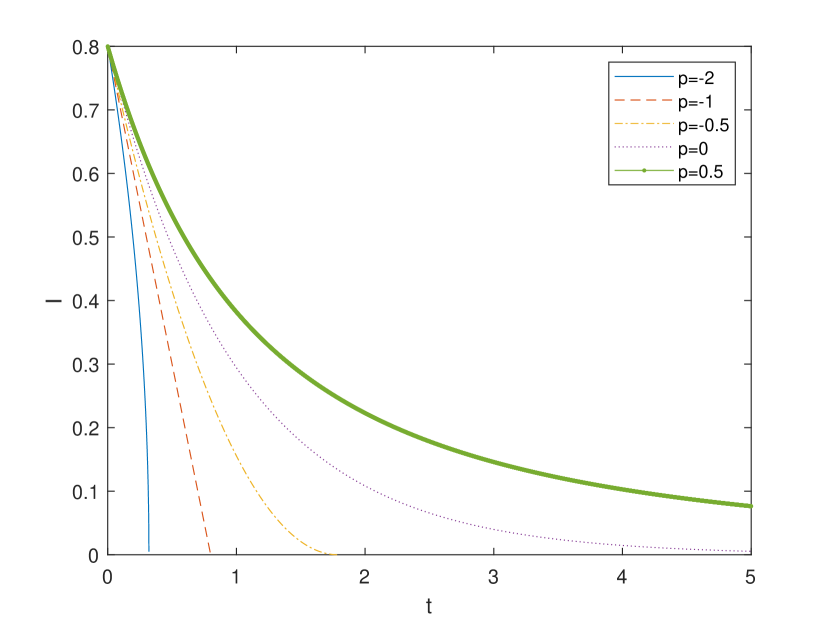
$\bullet$ Characterization of trend cycles - Fad, Fashion and Classic: Now, we explain how our model can characterize three different types of trends, namely, the fad, the fashion, and the classic, by proper choices of $p$ in the rejection rate $\beta$. We attempt to provide $\beta$ with clear mathematical reasoning. Since we are interested in the behavior after the trend reaches its peak, we consider only $t>T_{*}$, for which the equation for $I$ is (See (2.10))

$$I^{\prime}=\alpha SI-C_{*}I^{p+1}.$$

In the case $p=0$, the equation for $I$ becomes

$$I^{\prime}=\alpha SI-C_{*}I.$$

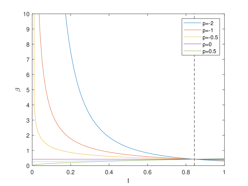
Since $\alpha$ has a lower and upper bound, we can expect that $I$ will behave like the usual SIR model, for which $I$ decays exponentially. When $p>0$, $I^{p+1}$ is much smaller than $I$ (since $I$ is normalized: $0\leq I<1$). Therefore, we can expect that the decay rate of $I$ will be much slower than that of $p=0$. Finally, in the case $p<0$, $I^{p+1}$ gets bigger as $I$ decreases to $0$. Moreover, since $SI$ is bounded by $I$, we expect that $C_{*}I^{p+1}$ will dominate over $\alpha SI$ so that the equation for $I$ in this case is governed by

$$I^{\prime}\approx-C_{*}I^{p+1},$$

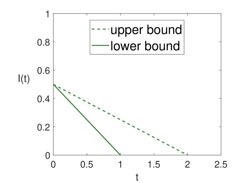
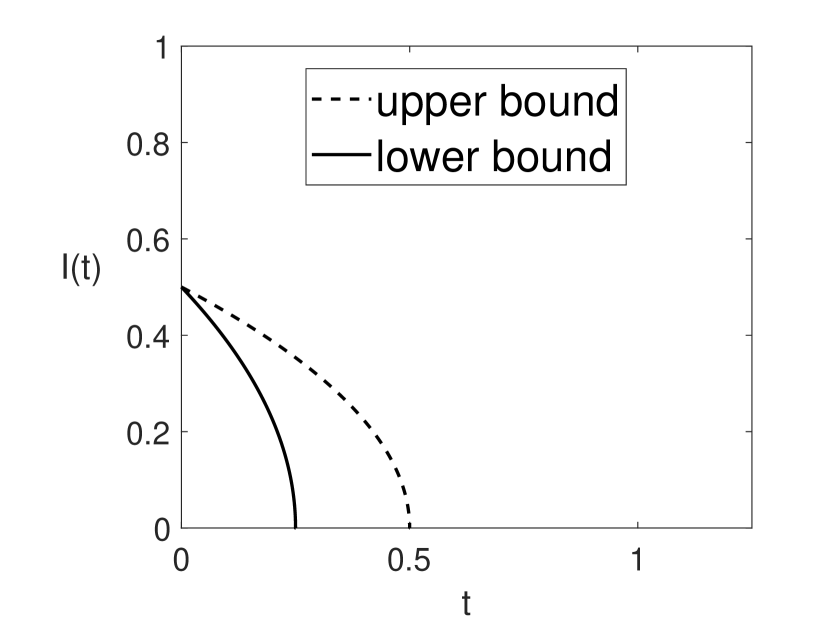
which vanishes in a finite time (see Fig. 3). This intuition leads to the following classification of the phase of $I$:

• $I$ vanishes in a finite time with a hard landing if $p\leq-1$,

• $I$ vanishes in a finite time with a soft landing if $-1<p<0$,

• $I$ decreases exponentially without vanishing in a finite time if $p=0$,

• $I$ decreases in a polynomial order if $p>0$,

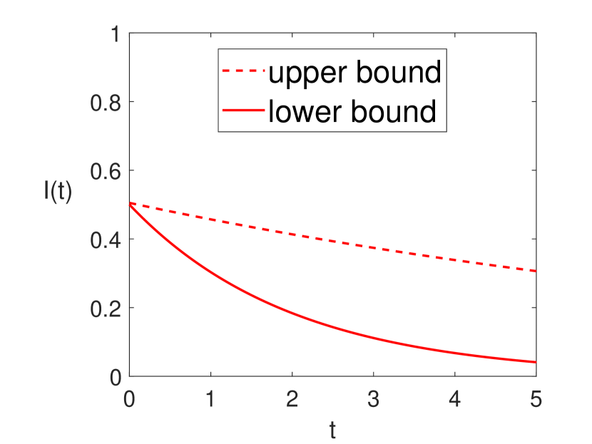
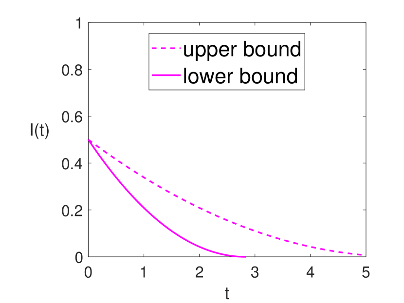
which will be verified analytically in Sec. 4, and numerically in Sec. 5. This provides us a way to draw a line between the fad, the fashion and the classic in a mathematically rigorous manner:

• Fad: The cycle experiences a finite time extinction with a hard landing if $p\leq-1$.

• Fast fashion: The cycle experiences a finite time extinction with a soft landing if $-1<p<0$.

• Fashion: The cycle declines exponentially fast if $p=0$.

• Classic: The cycle declines in a polynomial order if $p>0$.

This characterization matches well with our understanding that fad, fashion and classic are basically determined by the manner in which people reject a trend. This, in turn, is reflected in the slope’s steepness at the stage of decline and obsolescence, and the duration of the trend cycle. We also define th eperiodic case by

• Periodic: $p\geq 0$ with $\delta>0$.

Note that we only consider the case $p\geq 0$ for periodic case to prevent the situation where the trend cycle extincts before it enters the next cycle.

Remark 2.1.

We notice here the equation of $I$ consists of power-law. We may find a similarity between the behavior of the trend cycle and the motion of the non-Newtonian power-law fluid. It is shown in [2, Theorem 5.1] that

• the energy of the fluid vanishes in a finite time for $p<0$ (shear thinning fluid), which corresponds to Fad or Fast fashion,

• it decays exponentially for $p=0$ (Newtonian fluid, Navier-Stokes equations), which corresponds to Fashion, and

• it decays polynomially for $p>0$ (shear thickening fluid), which corresponds to Classic.

Figure 2. $p$-dependency of $I$. Here we solve the problem $I^{\prime}(t)=-I^{p+1}$ with $I(0)=0.8$.

Figure 3. Shape of function $\beta$ after $t=t_{*}$. Here $I\approx 0.84$ is the value of $I(t_{*})$.

3. Analysis of Classic, Fashion and Fad

In Section 2, we characterized the three different trends, Fad, Fashion and Classic, based on how the such a trend extinct as time goes.In this section, we verify them by deriving various decay estimates of $I$ depending on $p$. Before we state our main theorem, we need several technical lemmas. Throughout this section, we only consider the non-periodic case: $\delta=0$. We also recall that $m_{1}$ and $m_{3}$ denote the intensity of adopter/rejection in (2.3) and (2.6) respectively. For clarity of the proof, we fix $\ell_{\alpha}=\ell_{\beta}=0$ throughout this section.

Lemma 3.1.

Let

$$S(0)+I(0)+R(0)=1.$$

Then we have

$$S(t)+I(t)+R(t)=1.$$

for $t\geq 0$.

Proof.

We sum up the equations in the system (2.9) and observe that the right hand side of (2.9) cancels out each other. Then, we get

$$\frac{d}{dt}\left(S+I+R\right)=0,$$

which implies the desired result. ∎

In the following lemma, we consider the positivity of the solutions $S(t),~{}I(t),~{}R(t)$.

Lemma 3.2.

[Positivity of solutions] Assume that

(3.1) $$S(0)>0,\quad I(0)>0,\quad R(0)=0.$$

Then, we have

$$S(t)>0,\quad I(t)>0,\quad R(t)>0$$

for $0<t<T_{*}$.

Proof.

See Appendix. ∎

In the following lemma, we provide a sufficient condition under which the transition time $t_{*}$ becomes finite.

Lemma 3.3.

Assume

$$S(0)>0,\quad I(0)>0,\quad R(0)=0.$$

Suppose further that

$$\displaystyle m_{1}S(0)>2m_{3}.$$

Then the transition time $t_{*}>0$ is finite.

Lemma 3.4.

[Boundedness after $t_{*}$: $p<0$] Let $p<0$. Assume

$$S(0),~{}I(0),~{}R(0)>0$$

and

$$\displaystyle m_{1}S(0)>2m_{3}.$$

Then, there exists $t_{*}\leq\tau<T_{*}$ such that

$$I\leq\left(\frac{C_{*}}{2m_{1}}\right)I^{p+1}~{}\mbox{ for all }t>\tau.$$

Proof.

See Appendix. ∎

We now study two Bernouli type inequalities which will be crucially used in the analysis of long time behavior of the trend cycles.

Lemma 3.5.

[Bernoulli type differential inequality $(p>0)$] Set $p>0$. Assume that $I(t)>0$ and the following differential inequality holds for $T_{0}<t<T_{1}$:

$$\begin{split}&-bI^{p+1}\leq I^{\prime}\leq aI-bI^{p+1}.\end{split}$$

Then, we have

$$\begin{split}(I(T_{0}))^{-p}e^{-pa(t-T_{0})}+\frac{b}{a}\left(1-e^{-pa(t-T_{0})}\right)\leq(I(t))^{-p}\leq pb(t-T_{0})+(I(T_{0}))^{-p}.\end{split}$$

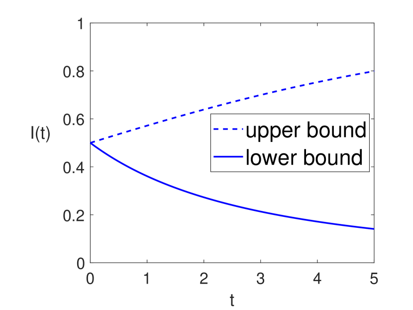
Theorem 3.6.

Let $\delta=0$. Assume

$$S(0),~{}I(0),~{}R(0)>0$$

and

$$\displaystyle m_{1}S(0)>2m_{3}.$$

Then we have

1. Classic: $(p>0):$ We have for $t>t_{*}$

   $$\begin{split}\frac{1}{\left(a_{*}^{-1/p}+b(t-t_{*})\right)^{\frac{1}{p}}}\leq I(t)&\leq\frac{1}{\left(a_{*}^{-1/p}-\left(a_{*}-c\right)\left(1-e^{-pm_{1}(t-t_{*})}\right)\right)^{\frac{1}{p}}}.\end{split}$$

2. Fashion: $(p=0)$. There exists $t_{2}>t_{*}$ such that, for $t>t_{*}$

   $$\begin{split}a_{*}e^{-C_{*}(t-t_{*})}\leq I(t)\leq a_{2}e^{-\varepsilon(t-t_{2})}.\cr\end{split}$$

3. Fad: $p<0$, we have for $\tau<t\leq T_{*}$

   $$\frac{1}{\left(a_{\tau}^{-p}+b(t-\tau)\right)^{\frac{1}{p}}}\leq I(t) \leq\frac{1}{\left(a_{\tau}^{-p}+\frac{b}{2}(t-\tau)\right)^{\frac{1}{p}}}.$$

Here, $a_{*}=I(t_{*})$, $a_{2}=\max\{a_{*},I(t_{2})\}$, $a_{\tau}=I(\tau)$, $b=pC_{*}$, $c=C_{*}/m_{1}$, $\varepsilon=\alpha(I(t_{2}))S(t_{2})-C_{*}$. The definition of $t_{2}$ is given in the proof.

(a) $p=0.5$

(b) $p=0$

(c) $p=-0.5$

(d) $p=-1$

(e) $p=-2$

Figure 4. Description of upper and Lower bounds for $I(t)$ for different values of $p$, which corresponds to the estimates in Theorem 3.6. In each figure, we use the upper bounds $U(t)$ and lower bounds $L(t)$ defined as follows:
(A) $U(t)=\left(\sqrt{2}-\left(\sqrt{2}-1\right)\left(1-e^{-t/4}\right)\right)^{-2}$ and $L(t)=\left(t/4+\sqrt{2}\right)^{-2}$
(B) $U(t)=\frac{1}{2}\exp(-0.1(t-0.1))$ and $L(t)=\frac{1}{2}\exp(-t/2)$
(C) $U(t)=(\sqrt{2}-t/4)^{2}$ and $L(t)=(\sqrt{2}-t/2)^{2}$
(D) $U(t)=1/2-t/4$ and $L(t)=1/2-t/2$
(E) $U(t)=((1/2)^{2}-t/2)^{1/2}$ and $L(t)=((1/2)^{2}-t)^{1/2}$

Proof.

$(1)$ From $0<S,I\leq 1$ and $\alpha\leq m_{1}$ we have

$$\begin{split}-C_{*}I^{p+1}\leq I^{\prime}&\leq m_{1}I-C_{*}I^{p+1}.\end{split}$$

Then, Lemma 3.5 gives

$$\begin{split}(I(t_{*}))^{-p}e^{-pm_{1}(t-t_{*})}+\frac{C_{*}}{m_{1}}\left(1-e^{-pm_{1}(t-t_{*})}\right)\leq(I(t))^{-p}\leq pC_{*}(t-t_{*})+(I(t_{*}))^{-p}.\end{split}$$

Recalling the definition of $C_{*}=\beta(I(t_{*}))(I(t_{*}))^{-p}$ and the fact that $\beta(I(t_{*}))\leq m_{3}<\frac{m_{1}S(0)}{2}<m_{1}$, we have

$$\begin{split}&(I(t_{*}))^{-p}e^{-pm_{1}(t-t_{*})}+\frac{C_{*}}{m_{1}}\left(1-e^{-pm_{1}(t-t_{*})}\right)\cr&=(I(t_{*}))^{-p}+C_{*}\left(\frac{1}{m_{1}}-\frac{1}{\beta(I(t_{*}))}\right)\left(1-e^{-pm_{1}(t-t_{*})}\right)\end{split}$$

Then, we have

$$\begin{split}(I(t_{*}))^{-p}-\left(I(t_{*}))^{-p}-\frac{C_{*}}{m_{1}}\right)\left(1-e^{-pm_{1}(t-t_{*})}\right)\leq(I(t))^{-p}\leq pC_{*}(t-t_{*})+(I(t_{*}))^{-p}.\end{split}$$

Rearranging this, we obtain the desired result.

$(2)$ By Lemma 3.2, for $p=0$ the following inequality holds

$$\begin{split}I^{\prime}&=\alpha(I)SI-C_{*}I\geq-C_{*}I\end{split}$$

due to the positivity of $S$, $\alpha$ and $I$. Thus, from Grönwall’s inequality, we obtain the desired lower bound. We turn to the proof of the upper bound. By an explicit computation, we see that

$$I^{\prime\prime}(t_{*})=\alpha(I(t_{*}))I(t_{*})S^{\prime}(t_{*})<0.$$

Therefore, $I^{\prime}(t)<0$ near $t_{*}$. Assume that there exists $t_{1}>t_{*}$ such that $I^{\prime}(t_{1})=0$ for the first time. This assumption implies

(3.2) $$\begin{split}I(t_{1})&<I(t_{*})\end{split}$$

On the other hand, from the fact that $S^{\prime}(t)=-\alpha(I)SI<0$, we get

(3.3) $$\begin{split}S(t_{1})<S(t_{*}).\end{split}$$

Now, combining (3.2), (3.3) and the fact that $\alpha$ is an increasing function of $I$, we find

$$0=I^{\prime}(t_{1})=(\alpha(I(t_{1}))S(t_{1})-C_{*})I(t_{1})<(\alpha(I(t_{*}))S(t_{*})-C_{*})I(t_{*})=I^{\prime}(t_{*})=0.$$

which is contradiction. Therefore,

$$I^{\prime}(t)<0\quad\mbox{ for all }t>t_{*},$$

That is, $I$ is strictly decreasing for $t>t_{*}$. This says that, if we take $t_{2}>t_{*}$ , then we have

$$\begin{split}I(t)&<I(t_{2}),\quad S(t)<S(t_{2})\quad\mbox{ for all }t>t_{2}\end{split}$$

This leads to

$$\alpha(I(t))S(t)-C_{*}<\alpha(I(t_{2}))S(t_{2})-C_{*}.$$

and

$$\begin{split}I^{\prime}(t)&=-(\alpha(I(t))S(t)-C_{*})I(t)<-(\alpha(I(t_{2}))S(t_{2})-C_{*})I(t),\quad t>t_{2}\end{split}$$

$(3)$ Since $0<S,I\leq 1$ and $\alpha\leq m_{1}$ we have from Lemma 3.4

(3.4) $$\begin{split}-C_{*}I^{p+1}\leq I^{\prime}\leq m_{1}I-C_{*}I^{p+1}\leq-\frac{C_{*}}{2}I^{p+1}.\end{split}$$

This gives the desired estimate. ∎

4. Numerical Tests

In this section, we provide numerical examples showing that our model (2.9) is able to capture the cyclic nature of a trend, and its three different modes: Fad, Fashion and Classic.

4.1. The influence of parameter $p$

We show that $p$ determines the speed of decline of a trend, which enables us to characterize Fad, Fashion and Classic. To clarify the role of $p$, we fix other parameters $m_{1}$, $m_{2}$, $\ell_{a}$ and $\ell_{b}$ in the adoption/rejection rate $\alpha$, $\beta$ by

(4.1) $$(m_{1},m_{2}) =(20,0.2),\,\ell_{a}=0,\quad(m_{3},m_{4})=(0.5,2),\,\ell_{b}=0$$

and set $\delta=0$. As initial data, we choose

(4.2) $$S(0)=0.98,\quad I_{1}(0)=0.02,\quad R(0)=0.$$

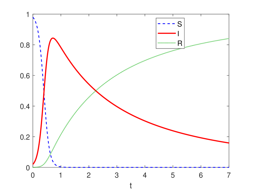
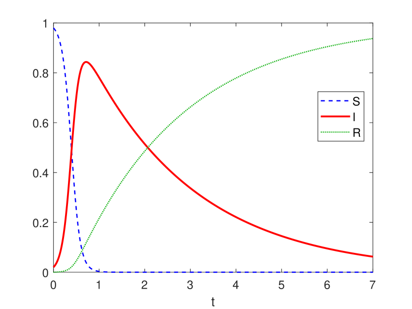
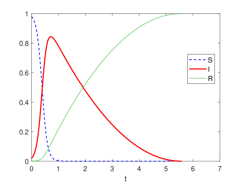
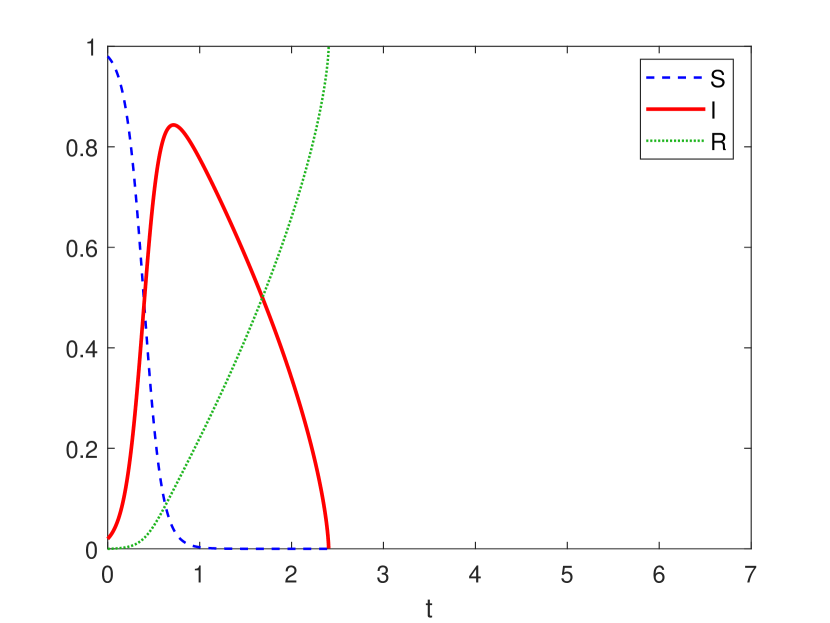
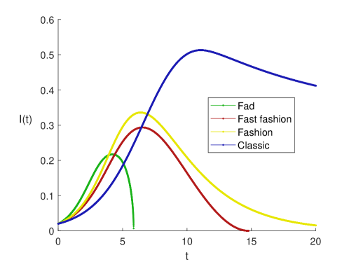
In Figure 5, we compare the profile of numerical solutions that correspond to various values of $p$. We observe that the choice $p>0$ leads to a very slow relaxation tendency of $I$ (Classic). The case of $p=0$ shows a much faster decay rate (Fashion). When $-1<p<0$, $I$ touches zero in a finite time with a soft landing (Fast fashion). In case of $p\leq-1$, $I$ extincts in a finite time with a hard landing (Fad).

(a) $p=0.5$

(b) $p=0$

(c) $p=-0.5$

(d) $p=-1.5$

Figure 5. Time evolution of $S,I,R$.

4.2. Expressive power of our model

In this test, we show that our model has expressive power strong enough to reproduce various trend cycles through an appropriate choice of parameters in the adoption rate $\alpha$ and the rejection rate $\beta$. For this, we reproduce a diagram quoted from [22] describing the trend cycle of Fad, Fashion and Classic (see Figure 1.).

Figure 6. Reproduction of the trend cycles corresponding to Fad, Fashion, and Classic in Figure 1. We also add the trend cycle of Fast fashion. See text for parameter values.

For each case, we use initial data

$$S(0)=98,~{}I(0)=2,~{}R(0)=0$$

with the following set of parameters:

• Fad:

  $$m_{1}=3,\,m_{2}=0.2,\,m_{3}=1,\,m_{4}=4,\,\ell_{\alpha}=0,\,\ell_{\beta}=0,\,p=-2.$$

• Fast fashion:

  $$m_{1}=2,\,m_{2}=0.03,\,m_{3}=0.6,\,m_{4}=1.5,\,\ell_{\alpha}=0,\,\ell_{\beta}=0,\,p=-0.5.$$

• Fashion:

  $$m_{1}=2,\,m_{2}=0.05,\,m_{3}=0.5,\,m_{4}=2\,,\ell_{\alpha}=0,\,\ell_{\beta}=0,\,p=0.$$

• Classic:

  $$m_{1}=1.2,\,m_{2}=0.03,\,m_{3}=0.2,\,m_{4}=0.5,\,\ell_{\alpha}=0,\,\ell_{\beta}=0,\,p=6.$$

4.3. Recurring cycle of a trend

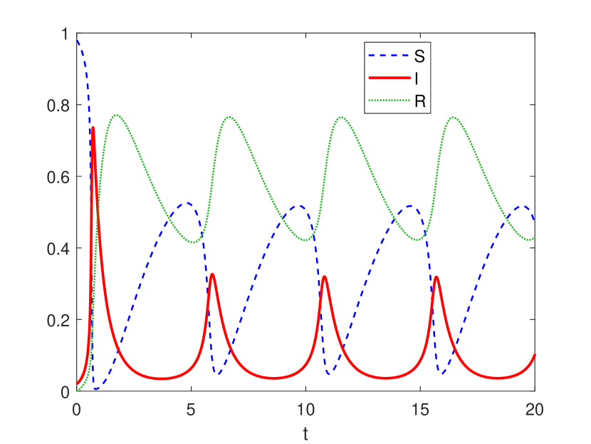
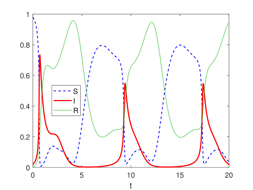
By taking positive value of $\delta$, our model can also describe a recurring cycle of the trend. The case $\delta>0$ corresponds to the situation where consumers (who have left a trend once) become potential consumers again. In order to clarify the role of $\delta$ in determining the scale and period of such a cycle, throughout this test we fix

$$(m_{1},m_{2},m_{3},m_{4})=(50,8,4,0.5),\,p=0,\,\ell_{\alpha}=0.3,\,\ell_{\beta}=0$$

and take different types of $\delta$. Here, we use the same initial data (4.2). In Figure 7, we observe that the choice of $\delta$ allows us to describe the recurring behavior of numerical solutions. The simulation shows that a time-dependent function $\delta(t)$ describes much sharper but less fluctuating solutions compared to the case for fixed $\delta$. We can take the recurrence rate $\delta$ to be a time-dependent function to describe a more complicated periodic trend cycle (Figure 7 (B)).

(a) $\delta=0.4$

(b) $\delta(t)=0.4+0.5\sin(\frac{\pi}{2}t-1)$

Figure 7. Recurrence of trend cycles depending on $\delta$.

5. Conclusion

In this work, we suggest a system of differential equations that quantitatively model the evolution of a trend through the consideration of underlying dynamics between trend participants. Our model captures five stages of a trend cycle, namely, the onset, rise, peak, decline, and obsolescence. It also provides a mathematical criterion to divide Fad, Fashion and Classic. We also prove various mathematical properties of our model, and provide simulations to justify the modeling. Note that we have investigated a mono-fashion model, where only one trend is considered for simplicity. Extension of such mono-fashion model into a multi-fashion model, where the differentiation into a sub-fashion is taken into consideration, will be an interesting topic. This is our upcoming work.

Acknowledgement:

Bae is supported by the Basic Research Program through the National Research Foundation of Korea (NRF) funded by the Ministry of Education and Technology (NRF-2021R1A2C1093383), Cho (RS-2022-00166144), Yoo by Ajou University Research Fund, and Yun by Samsung Science and Technology Foundation under Project Number SSTF-BA1801-02.

Appendix A Proof of Lemma 3.2

Since $S(t)=S(0)e^{-\int^{t}_{0}\alpha I(s)ds}$ and $R(t)=\beta SI$, it is enough to show that $I(t)>0$. $(1)$ Case of $t<t_{*}$: In this case, we have

$$I^{\prime}(t)\geq-\beta(I)I\geq-m_{3}I.$$

Therefore

$$I(t)\geq\alpha SI-\beta I\geq-\beta I\geq e^{-m_{3}t}I(0)>0.$$

This gives the desired result.
$(2)$ Case of $t>t_{*}$ and $p\geq 0$: In this case, we use $I^{p+1}\leq I$ to get

$$I^{\prime}(t)=\alpha SI-C_{*}I^{p+1}\geq-C_{*}I^{p+1}\geq-C_{*}I(t)$$

so that $I(t)\geq I(t_{*})e^{-C_{*}(t-t_{*})}>0.$
$(3)$ Case of $t_{*}<t<T_{*}$ and $p<0$: In this case, $I$ satisfies

$$I^{\prime}(t)=\alpha SI-C_{*}I^{p+1}\geq-C_{*}I^{p+1}$$

which yields:

$$I(t)\geq\left(I^{-p}(t_{*})+pm_{3}(t-t_{*})\right)^{-\frac{1}{p}}>0.$$

Appendix B Proof of Lemma 3.3

Since $\displaystyle m_{1}S(0)>2m_{3}$, $I$ increases initially:

$$\begin{split}I^{\prime}(0)&=\alpha(I(0))I(0)S(0)-\beta(I(0))I(0)\geq\frac{m_{1}}{2}I(0)S(0)-m_{3}I(0)\geq\left(\frac{m_{1}}{2}S(0)-m_{3}\right)I(0)>0.\end{split}$$

Assume $I^{\prime}(t)>0$ for all $t$ so that

$$\begin{split}I(t)&\geq I(0)>0\quad\mbox{ for }t>0\end{split}$$

However, this implies that

$$S(t)\leq S(0)e^{-\int_{0}^{t}\alpha I(0)ds}\leq S(0)e^{-\frac{m_{1}}{2}I(0)t}\to 0$$

as $t$ goes to $\infty$. That is, there is a sufficiently large time $T>0$ such that

$$S(t)<\frac{m_{3}}{4m_{1}}<\frac{1}{8}$$

for $t>T$. Hence

$$\begin{split}I^{\prime}&\leq(m_{3}/4)I-(m_{3}/2)I<0.\end{split}$$

This contradicts the assumption. Therefore, $t_{*}$ is finite.

Appendix C Proof of Lemma 3.4

We first make the following claim:
Claim: Choose any $I_{*}$ such that $0<I^{*}<I(t_{*})$, then $I(t)$ becomes smaller than $I^{*}$ in a finite time.
Proof of the claim: To prove the claim, suppose contrarily that $I^{*}\leq I(t)\leq 1$ for all $t>t_{*}$. Under this assumption, $S$ satisfies

$$S(t)=S(t_{*})e^{-\int_{0}^{t}\alpha(I(s))I(s)ds}\leq S(t_{*})e^{-\int_{t_{*}}^{t}\frac{m_{1}}{2}I(s)ds}\leq S(t_{*})e^{-\frac{m_{1}}{2}I_{*}(t-t_{*})}.$$

Therefore, for sufficiently large $t$, we have

(C.1) $$\begin{split}I^{\prime}&=\alpha(I)SI-C_{*}I^{p+1}\leq\big{(}m_{1}S-C_{*}\big{)}I\leq-\frac{C_{*}}{2}I.\end{split}$$

This implies that $I$ decreases exponentially fast, which contradicts the assumption that $I(t)\geq I^{*}>0$ for all $t>t_{*}$. This proves the claim.

Now, from the definition of $C_{*}$ given in the definition of $\beta$, we see that

$$\left(\frac{C_{*}}{2m_{1}}\right)^{-1/p}\leq\left(\frac{m_{3}}{2m_{1}}\left(I(t_{*})\right)^{-p}\right)^{-1/p}\leq I(t_{*})$$

In the last inequality, we used $\displaystyle m_{3}/m_{1}<S(0)/2<1$. Therefore, thanks to the claim, we can find $\tau>t_{*}$ such that

$$I(\tau)=\left(\frac{C_{*}}{2m_{1}}\right)^{-\frac{1}{p}}.$$

Let $\bar{t}>\tau$ be the first time such that $I(\bar{t})=I(\tau)$. Then, $I(t)<I(\tau)$ holds for $\tau<t<\bar{t}$. Hence

$$\begin{split}I^{\prime}(t)\leq m_{1}I(t)-C_{*}I(t)^{p+1}<m_{1}I(t)-C_{*}\{I(\tau)\}^{p}I(t)=m_{1}I(t)-\left(2m_{1}/C_{*}\right)I(t)\leq-m_{1}I(t),\end{split}$$

which implies $I(\bar{t})$ is strictly less than $I(\tau)$ on $\tau<t<\bar{t}$. This contracts the assumption. Therefore, for all $t\geq\tau$ we have $I(t)\leq I(\tau)$, which is equivalent to

$$I(t)\leq\frac{C_{*}}{2m_{1}}\left(I(t)\right)^{p+1}.$$

Appendix D Proof of Lemma 3.5

Dividing both sides of the inequality by $I^{p+1}$, we get

$$\begin{split}-b\leq\left(\frac{1}{-p}I^{-p}\right)^{\prime}&\leq aI^{-p}-b.\end{split}$$

The second inequality is trivial. For the first one, we apply Grönwall’s lemma to obtain

$$\begin{split}I^{-p}(t)&\geq I^{-p}(T_{0})e^{-pa(t-T_{0})}+\frac{b}{a}\left(1-e^{-pa(t-T_{0})}\right),\end{split}$$

which completes the proof.

References

- [1] Ahmetolan S., Bilge A.H., Demirci A., Peker-Dobie A., Ergonul O. (2020). What can we estimate from fatality and infectious case data using the susceptible-infected-removed (SIR) model? A case study of Covid-19 pandemic, Front. Med., 7, 556366.
- [2] Bae, H.-O. (1999). Existence, regularity, and decay rate of solutions of non-Newtonian flow. J. Math. Anal. Appl. 231(2), 467–-491.
- [3] Beckley R, Weatherspoon C, Alexander M, Chandler M, Johnson A, Bhatt G. S. (2013). Modeling epidemics with differential equations. Tennessee State University Internal Report.
- [4] Berger, J. Mens, GL (2009). How adoption speed affects the abandonment of cultural tastes. PNAS 106(20), 8146 - 8150.
- [5] Bhardwaj V., Fairhurst A. (2010). Fast fashion: response to changes in the fashion industry, The international review of retail, distribution and consumer research, 20(1), 165-173.
- [6] Cachon, G. P., Swinney, R. (2011). The value of fast fashion: Quick response, enhanced design, and strategic consumer behavior. Management science, 57(4), 778-795.
- [7] Callahan, C. E. (2012). Fashion Frustrated: Why the Innovative Design Protection Act Is a Necessary Step in the Right Direction, but Not Quite Enough. Brook. J. Corp. Fin. & Com. L., 7, 195.
- [8] Cho, H. S., Lee, J. (2005). Development of a macroscopic model on recent fashion trends on the basis of consumer emotion. International Journal of Consumer Studies, 29(1), 17-33.
- [9] Ewing, E., Mackrell, A. (2014). History of 20th century fashion. Batsford.
- [10] Hansen, K. T. (2004). The world in dress: Anthropological perspectives on clothing, fashion, and culture. Annu. Rev. Anthropol., 33, 369-392.
- [11] Harko, T., Lobo, F. S., Mak, M. (2014). Exact analytical solutions of the Susceptible-Infected-Recovered (SIR) epidemic model and of the SIR model with equal death and birth rates. Applied Mathematics and Computation, 236, 184-194.
- [12] Hemphill C. S., Suk J. (2009). The Law, Culture, and Economics of Fashion, Stan. L. Rev., 61, 1147.
- [13] Gopagoni D., Lakshmi P. V. (2020). Susceptible, infectious and recovered (SIR model) predictive model to understand the key factors of COVID-19 transmission Int. J. Adv. Comput. Sci. Appl., 11(9), 296-302
- [14] Kaiser, S. B. (1997). The social psychology of clothing: Symbolic appearances in context. Fairchild Books.
- [15] Kermack, W. O., McKendrick, A. G. (1927). A contribution to the mathematical theory of epidemics. Proceedings of the royal society of london. Series A, Containing papers of a mathematical and physical character, 115(772), 700-721.
- [16] Kim, A. J., Ko, E. (2010). Impacts of luxury fashion brand’s social media marketing on customer relationship and purchase intention. Journal of Global fashion marketing, 1(3), 164-171.
- [17] Kim, K. H. (2011). Virtual hallyu. In Virtual Hallyu. Duke University Press.
- [18] King, C. W., Ring, L. J. (1980). The dynamics of style and taste adoption and diffusion: contributions from fashion theory. ACR North American Advances.
- [19] Kröger, M., Schlickeiser, R. (2020). Analytical solution of the SIR-model for the temporal evolution of epidemics. Part A: time-independent reproduction factor. Journal of Physics A: Mathematical and Theoretical, 53(50), 505601.
- [20] Law K.B., Peariasamy K.M., Gill B.S., Singh S., Sundram B.M., Rajendran K., Dass S.C., Lee Y.L., Goh P.P., Ibrahim H., Abdullah N.H. (2020). Tracking the early depleting transmission dynamics of COVID-19 with a time-varying SIR model. Sci. Rep., 10(1), 1-11.
- [21] Lee, S. C. (2022). Magical capitalism, gambler subjects: South Korea’s bitcoin investment frenzy. Cultural Studies, 36(1), 96-119.
- [22] Lynch, A., Strauss, M. (2007). Changing fashion: a critical introduction to trend analysis and cultural meaning. Berg.
- [23] McCracken, G. D. (1990). Culture and consumption: New approaches to the symbolic character of consumer goods and activities (Vol. 1). Indiana University Press.
- [24] Mohr, I. (2013). The impact of social media on the fashion industry. Journal of applied business and economics, 15(2), 17-22.
- [25] Neher R.A., Dyrdak R., Valentin D., Hodcroft E.B., Albert J. (2020). Potential impact of seasonal forcing on a SARS-CoV-2 pandemic Swiss Med. Wkly., 150, p. w20224
- [26] Pesendorfer, W. (1995). Design innovation and trend cycles. The american economic review, 771-792.
- [27] Ritch, E. L. (2014). Extending sustainability from food to fashion consumption: the lived experience of working mothers. International Journal of Management Cases, 16(2), 17-31.
- [28] Schlickeiser, R., Kröger, M. (2021). Analytical solution of the SIR-model for the temporal evolution of epidemics: Part B. Semi-time case. Journal of Physics A: Mathematical and Theoretical, 54(17), 175601.
- [29] Simmel, G. (1957). Fashion. American journal of sociology, 62(6), 541-558.
- [30] Vanderploeg, A., Lee, S. E., Mamp, M. (2017). The application of 3D printing technology in the fashion industry. International Journal of Fashion Design, Technology and Education, 10(2), 170-179.
- [31] Van der Veen, A. M. (2012). The Dutch tulip mania: The social foundations of a financial bubble. Department of Government College of William & Mary.
- [32] Yoganarasimhan, H. (2017). Identifying the presence and cause of fashion cycles in data. Journal of Marketing Research, 54(1), 5-26.