Anisotropic modified Crouzeix–Raviart finite element method for the stationary Navier–Stokes equation

Abstract

We study an anisotropic modified Crouzeix–Raviart finite element method to the rotational form of the stationary incompressible Navier–Stokes equation with large irrotational body forces. We present an anisotropic $H^{1}$ error estimate for the velocity of a modified Crouzeix–Raviart finite element method for the Navier–Stokes equation. The modified Crouzeix–Raviart finite element scheme was obtained using a lifting operator that maps the velocity test functions to $H(\mathop{\mathrm{div}};\Omega)$-conforming finite element spaces. Because no shape-regularity mesh conditions are imposed, anisotropic meshes can be used for analysis. The core idea of the proof involves using the relation between the Raviart–Thomas and Crouzeix–Raviart finite element spaces. Furthermore, we present a discrete Sobolev inequality under a semi-regular mesh condition to estimate the stability of the proposed method and confirm the obtained results through numerical experiments.

1 Introduction

Let $\Omega\subset\mathbb{R}^{d}$, $d\in\{2,3\}$ be a bounded polyhedral domain. The stationary Navier–Stokes problem is to find $(u,p_{0}):\Omega\to\mathbb{R}^{d}\times\mathbb{R}$ such that

$$\displaystyle-\nu\varDelta u+(u\cdot\nabla)u+\nabla p_{0}=f\quad\text{in $\Omega$},\quad\mathop{\mathrm{div}}u=0\quad\text{in $\Omega$},\quad u=0\quad\text{on $\partial\Omega$},$$ (1.1)

where $\nu$ is a nonnegative parameter, and $f:\Omega\to\mathbb{R}^{d}$ is a given function. We use the standard notation for Lebesgue and Sobolev spaces with associated norms ErnGue04 ; ErnGue21a ; ErnGue21b ; ErnGue21c ; GirRav86 ; Gri11 ; Joh16 ; Soh01 . We define the curl operator GirRav86 ; Joh16 as

$$\displaystyle\mathop{\mathrm{curl}}\varphi=\left(\frac{\partial\varphi}{\partial x_{2}},-\frac{\partial\varphi}{\partial x_{1}}\right)^{T},\quad\mathop{\mathrm{curl}}u=\frac{\partial u_{2}}{\partial x_{1}}-\frac{\partial u_{1}}{\partial x_{2}}$$

for distributions $\varphi$ of $\mathscr{D}^{\prime}(\Omega)$ and $u$ of $\mathscr{D}^{\prime}(\Omega)^{2}$ when $d=2$,, and

$$\displaystyle\mathop{\mathrm{curl}}u=\left(\frac{\partial u_{3}}{\partial x_{2}}-\frac{\partial u_{2}}{\partial x_{3}},\frac{\partial u_{1}}{\partial x_{3}}-\frac{\partial u_{3}}{\partial x_{1}},\frac{\partial u_{2}}{\partial x_{1}}-\frac{\partial u_{1}}{\partial x_{2}}\right)^{T}$$

for the distribution $u$ of $\mathscr{D}^{\prime}(\Omega)^{3}$ when $d=3$. These operators lead to

$$\displaystyle(\mathop{\mathrm{curl}}u)\times u+\frac{1}{2}\nabla(u^{T}u)=(u\cdot\nabla)u.$$

This paper studies the rotation form of the stationary Navier–Stokes equation (1.1) as follows. Find $(u,p):\Omega\to\mathbb{R}^{d}\times\mathbb{R}$ such that

$$\displaystyle-\nu\varDelta u+(\mathop{\mathrm{curl}}u)\times u+\nabla p=f\quad\text{in $\Omega$},\quad\mathop{\mathrm{div}}u=0\quad\text{in $\Omega$},\quad u=0\quad\text{on $\partial\Omega$},$$ (1.2)

where $p$ represents the Bernoulli pressure $p:=p_{0}+\frac{1}{2}u^{T}u$.

Mixed finite element methods are commonly used in numerical analysis to solve incompressible Navier–Stokes equations. These methods require the discrete inf-sup condition to guarantee stability and a unique solution. However, finding Stokes elements that satisfy the discrete inf-sup condition for anisotropic mesh partitions is challenging. Furthermore, even on regular shape meshes, most of the Stokes elements of the inf-sup stable finite element spaces consider divergence-free discrete function spaces, $V_{h,\mathop{\mathrm{div}}}$, which is nonconforming in the space of divergence-free weak functions, $V_{\mathop{\mathrm{div}}}$. When Stokes elements are used, the velocity error depends on the pressure error ((Joh16, , Theorem 6.30, Corollary 6.33)), that is,

$$\displaystyle|u-u_{h}|_{V_{h}}\leq c_{1h}\inf_{v_{h}\in V_{h}}|u-v_{h}|_{V_{h}}+c_{2h}\nu^{-1}\inf_{q_{h}\in Q_{h}}\|p-q_{h}\|_{Q_{h}},$$

where $u_{h}$ denotes the discrete solution of $u$, $V_{h}$ and $Q_{h}$ are the discrete velocity and pressure spaces, respectively. If $\nu$ is small and the pressure error is large, classical mixed finite element methods lead to poor velocity approximations, even when finer meshes are used. This phenomenon is known as poor conservation of mass.

To overcome this difficulty, using $H(\mathop{\mathrm{div}};\Omega):=\{v\in L^{2}(\Omega)^{d}:\ \mathop{\mathrm{div}}v\in L^{2}(\Omega)\}$-conforming velocity lifting operator $\mathcal{L}_{h}$, the schemes are modified when $V_{h,\mathop{\mathrm{div}}}\not\subset V_{\mathop{\mathrm{div}}}$ by replacing the velocity test function $v_{h}$ in the discrete momentum equation with the lifting operator $\mathcal{L}_{h}(v_{h})$. This idea was presented by Linke Lin14 for the Stokes equation and has been widely applied in finite element methods Johetal17 ; Ledetal17 ; LinMatTob16 ; QuiPie20 ; YanHeZha22 . One says that the discretisation is pressure robust or well-balanced. In Lin14 , as the Stokes element, the Crouzeix–Raviart (CR) finite element space for velocity and elementwise constant discontinuous space for pressure were used for the analysis. The corresponding velocity-lifting operator maps the CR velocity test functions to the lowest-order Raviart–Thomas (RT) finite element space that conforms to $H(\mathop{\mathrm{div}};\Omega)$. The modified CR finite element method leads to a pressure-independent velocity error estimate under the shape-regular mesh condition of the form

$$\displaystyle|u-u_{h}|_{V_{h}}\leq ch|u|_{H^{2}(\Omega)^{d}}.$$

The Navier–Stokes equations have various discrete trilinear forms for the nonlinear convection term, e.g., the convective form, the skew-symmetric form, and the (skew-symmetric) rotational form with modified pressure (e.g., see Joh16 ). For continuous problems, the nonlinear convection terms do not contribute to stability estimates. However, the discrete convective form affects discrete stability estimates and uniqueness for the velocity. Meanwhile, because the space $H(\mathop{\mathrm{div}};\Omega)$ is not in $H^{1}(\Omega)^{d}$, the pressure-robust schemes with the skew-symmetric form are not possible for the conforming Stokes elements. In LinMer16a , Linke and Merdon proposed the pressure-robust method for the rotation form of the Navier–Stokes equation using the standard discrete rotation form with an additional term which preserves the skew-symmetry. Later, in QuiPie20 , the pressure-robust method of the hybrid high-order (HHO) for the skew-symmetric rotation form of the stationary Navier–Stokes equation was studied. In YanHeZha22 , the high-order pressure-robust method of the skew-symmetric rotation form of the stationary Navier–Stokes equation was proposed.

The main contributions of this study are as follows. We study the modified CR finite element method to the skew-symmetric rotation form of the stationary incompressible Navier–Stokes equation on anisotropic mesh partitions. We present the discrete Sobolev inequality and the $H^{1}$ error estimate of the modified CR finite element method using a lifting operator to the lowest-order RT finite element space under a relaxed mesh condition (3.2).

The remainder of this paper is organised as follows. Section 2 introduces the features of the Navier–Stokes equation in a continuous setting. Section 3 discusses the interpolation error estimates and finite element spaces. Section 4 introduces the modified CR finite element scheme and presents the main theorem of this study. Section 5 presents the numerical results.

Throughout this study, $c$ denotes a constant independent of $h$ (defined later) unless specified otherwise. The $c$ values can vary in different contexts.

2 Continuous problem

2.1 Weak formulation

In finite element analysis, we derive a variational form of the continuous problem (1.2). We set $X:=H^{1}(\Omega)^{d}$, $V:=H_{0}^{1}(\Omega)^{d}$, and $Q:=L^{2}_{0}(\Omega):=\left\{q\in L^{2}(\Omega):\ \int_{\Omega}qdx=0\right\}$ with norms $\|\cdot\|_{X}:=\|\cdot\|_{H^{1}(\Omega)^{d}}$. $|\cdot|_{V}:=|\cdot|_{H^{1}(\Omega)^{d}}$, and $\|\cdot\|_{Q}:=\|\cdot\|_{L^{2}(\Omega)}$, respectively. The rotation form of the nonlinear term is defined as

$$\displaystyle a_{\mathop{\mathrm{rot}}}(u,v,w) :=\int_{\Omega}(\mathop{\mathrm{curl}}u)\times v\cdot wdx\quad\forall u,v,w\in X.$$

Note that $a_{\mathop{\mathrm{rot}}}(u,v,v)=0$ for any $u,v\in X$. $a(_{\cdot},_{\cdot}):X\times X\to\mathbb{R}$, and $b(_{\cdot},_{\cdot}):X\times L^{2}(\Omega)\to\mathbb{R}$ denote bilinear forms defined as

$$\displaystyle a(v,w) :=\int_{\Omega}\nabla v:\nabla wdx=\sum_{i=1}^{d}\int_{\Omega}\nabla v_{i}\cdot\nabla w_{i}dx,$$

$$b(v,q) :=-\int_{\Omega}\mathop{\mathrm{div}}vqdx,$$

for any $(v,w)\in X\times X$ and $(v,q)\in X\times L^{2}(\Omega)$. For any $f\in L^{2}(\Omega)^{d}$, the variational formulation for the Navier–Stokes equations (1.2) is to find $(u,p)\in V\times Q$ such that

$$\displaystyle\nu a(u,v)+a_{\mathop{\mathrm{rot}}}(u,u,v)+b(v,p) =\int_{\Omega}f\cdot vdx\quad\forall v\in V,$$ (2.1a)

$$b(u,q) =0\quad\forall q\in Q.$$ (2.1b)

The space of the divergence-free weak function is defined as $V_{\mathop{\mathrm{div}}}:=\{v\in V:\ b(v,q)=0\ \forall q\in Q\}$. The reduced problem in (2.1) is as follows: Find $u\in V_{\mathop{\mathrm{div}}}$ such that

$$\displaystyle\nu a(u,v)+a_{\mathop{\mathrm{rot}}}(u,u,v) =\int_{\Omega}f\cdot vdx\quad\forall v\in V_{\mathop{\mathrm{div}}}.$$ (2.2)

2.2 Helmholtz projection

Setting $H_{*}^{1}(\Omega):=H^{1}(\Omega)\cap L^{2}_{0}(\Omega)$ and $\mathcal{H}=\{v\in L^{2}(\Omega)^{d}:\ \mathop{\mathrm{div}}v=0,\ v|_{\partial\Omega}\cdot n=0\}$, where $\mathop{\mathrm{div}}v=0$ and $v|_{\partial\Omega}\cdot n=0$ signifies that $\int_{\Omega}(v\cdot\nabla)qdx=0$ for any $q\in H_{*}^{1}(\Omega)$. Then, each $f\in L^{2}(\Omega)^{d}$ has a unique decomposition:

$$\displaystyle f=f_{0}+\nabla\phi,\quad f_{0}\in\mathcal{H},\quad\phi\in H_{*}^{1}(\Omega),$$

For example, refer (ErnGue21c, , Lemma 74.1) and GirRav86 ; Joh16 ; Soh01 . The $L^{2}$-orthogonal projection $P_{\mathcal{H}}:L^{2}(\Omega)^{d}\to\mathcal{H}$ resulting from this decomposition is defined as $P_{\mathcal{H}}f:=f_{0}$.

Let $f\in L^{2}(\Omega)^{d}$. For any $v\in H^{1}(\Omega)^{d}$ which is divergence-free and vanishes at the boundary, it holds that

$$\displaystyle\int_{\Omega}f\cdot vdx =\int_{\Omega}P_{\mathcal{H}}f\cdot vdx.$$ (2.3)

The Poincaré inequality yields

$$\displaystyle\left|\int_{\omega}P_{\mathcal{H}}f\cdot vdx\right| \leq\|P_{\mathcal{H}}f\|_{L^{2}(\Omega)^{d}}\|v\|_{L^{2}(\Omega)^{d}}\leq C_{P}\|P_{\mathcal{H}}f\|_{L^{2}(\Omega)^{d}}|v|_{V},$$ (2.4)

where $C_{P}$ denotes the Poincaré constant. Furthermore, for any $u\in W^{1,4}(\Omega)^{d}$, $(\mathop{\mathrm{curl}}u)\times u\in L^{2}(\Omega)^{d}$ holds. Then,

$$\displaystyle a_{\mathop{\mathrm{rot}}}(u,u,v)=\int_{\Omega}(\mathop{\mathrm{curl}}u)\times u\cdot vdx =\int_{\Omega}P_{\mathcal{H}}\left((\mathop{\mathrm{curl}}u)\times u\right)\cdot vdx.$$ (2.5)

2.3 Existence, uniqueness, and stability of a solution

This section states notable points regarding our continuity problem. These are the key features in the design of finite element schemes.

For the trilinear form $a_{\mathop{\mathrm{rot}}}$, from Sobolev embedding theorem $H^{1}(\Omega)\hookrightarrow L^{4}(\Omega)$, and Hölder inequality with exponents $(\frac{1}{4},\frac{1}{2},\frac{1}{4})$ we obtain

$$\displaystyle|a_{\mathop{\mathrm{rot}}}(u,v,w)|\leq N|u|_{V}|v|_{V}|w|_{V}\quad\forall u,v,w\in V,$$ (2.6)

where $N$ is a positive constant independent of $u$, $v$, and $w$. Additionally, the bilinear form $a$ is continuous on $V\times V$ and coercive on $V_{\mathop{\mathrm{div}}}\times V_{\mathop{\mathrm{div}}}$. The bilinear form $b$ is continuous on $V\times Q$, and there exists a positive constant $\beta$ such that

$$\displaystyle\inf_{q\in Q}\sup_{v\in V}\frac{b(v,q)}{|v|_{V}\|q\|_{Q}}\geq\beta\mathop{\textgreater}0.$$ (2.7)

For example, refer to (Joh16, , Theorem 3.46), (ErnGue21b, , Lemma 53.9), and (GirRav86, , Lemma 4.1).

Theorem 1

For any $f\in L^{2}(\Omega)^{d}$, there exists at least one solution of the variational formulation (2.1) for the Navier–Stokes equations.

Proof

The proof of the existence is found in (GirRav86, , Chap. IV. Theorem 2.1), (Tem01, , Chap. II, Theorem 1.2). ∎

We are interested in the uniqueness of the velocity solution. The result is slightly different compared to the usual.

Theorem 2

For $f\in L^{2}(\Omega)^{d}$, if

$$\displaystyle\frac{NC_{P}}{\nu^{2}}\|P_{\mathcal{H}}f\|_{L^{2}(\Omega)^{d}}\mathop{\textless}1$$ (2.8)

holds, the problem (2.2) has a unique solution $u\in V_{\mathop{\mathrm{div}}}$.

Proof

We provide proof of the uniqueness as follows: Let $u\in V_{\mathop{\mathrm{div}}}$ be the solution of the problem (2.2). Setting $v:=u$ in (2.2) and using (2.4), we obtain,

$$\displaystyle\nu|u|^{2}_{V}=\int_{\omega}P_{\mathcal{H}}f\cdot udx\leq C_{P}\|P_{\mathcal{H}}f\|_{L^{2}(\Omega)^{d}}|u|_{V},$$

which leads to

$$\displaystyle|u|_{V}\leq\frac{C_{P}}{\nu}\|P_{\mathcal{H}}f\|_{L^{2}(\Omega)^{d}},$$ (2.9)

where $C_{P}$ denotes the Poincaré constant. Let $u_{1}$ and $u_{2}$ be the solutions of the problem (2.2). We set $u:=u_{1}-u_{2}$ and subtract the problem (2.2) corresponding to $u_{1}$ and $u_{2}$. Then,

$$\displaystyle\nu a(u,v)+a_{\mathop{\mathrm{rot}}}(u_{2},u,v)+a_{\mathop{\mathrm{rot}}}(u,u_{1},v)=0\quad\forall v\in V_{\mathop{\mathrm{div}}}.$$ (2.10)

Setting $v:=u$ in (2.10), with (2.6) and (2.9), it holds that

$$\displaystyle\nu|u|^{2}_{V} =-a_{\mathop{\mathrm{rot}}}(u,u_{1},u)\leq N|u|^{2}_{V}|u_{1}|_{V}\leq\frac{NC_{P}}{\nu}\|P_{\mathcal{H}}f\|_{L^{2}(\Omega)^{d}}|u|^{2}_{V},$$

which leads to

$$\displaystyle\left(1-\frac{NC_{P}}{\nu^{2}}\|P_{\mathcal{H}}f\|_{L^{2}(\Omega)^{d}}\right)|u|^{2}_{V}\leq 0.$$

If (2.8) holds, this inequality implies that $u_{1}=u_{2}$. ∎

Remark 1

The stability estimate (2.9) is sharper than the classical estimate, $|u|_{V}\leq\frac{C_{p}}{\nu}\|f\|_{L^{2}(\Omega)^{s}}$. The stability estimate for the pressure follows from the inf-sup condition (2.7). Changing the right hand side of (2.2) as $f\to f+\nabla\phi$ for $\phi\in H_{*}^{1}(\Omega)$ yields

$$\displaystyle\nu|u|_{V}\leq C_{P}\|P_{\mathcal{H}}(f+\nabla\phi)\|_{L^{2}(\Omega)^{d}}=C_{P}\|P_{\mathcal{H}}f\|_{L^{2}(\Omega)^{d}},$$

because $P_{\mathcal{H}}(\nabla\phi)=0$. Therefore, the velocity is unaffected by the irrotational part of the force.

3 Interpolation error estimates

For anisotropic interpolation errors on anisotropic meshes, our strategy is proposed in Ish21 ; Ish23a ; IshKobTsu23a .

3.1 Notation

For $k\in\mathbb{N}_{0}:=\mathbb{N}\cup\{0\}$, $\mathbb{P}^{k}(T)$ is spanned by the restriction to $T$ by polynomials in $\mathbb{P}^{k}$, where $\mathbb{P}^{k}$ denotes the space of polynomials with at most $k$ degrees. In addition, we introduce the Jensen-type inequality, (ErnGue21a, , Exercise 12.1). Let $r,s$ be two nonnegative real numbers and $\{x_{i}\}_{i\in I}$ be a finite sequence of nonnegative numbers. It then holds that

$$\displaystyle\begin{cases}\left(\sum_{i\in I}x_{i}^{s}\right)^{\frac{1}{s}}\leq\left(\sum_{i\in I}x_{i}^{r}\right)^{\frac{1}{r}}\quad\text{if $r\leq s$},\\ \left(\sum_{i\in I}x_{i}^{s}\right)^{\frac{1}{s}}\leq\mathop{\rm{card}}(I)^{\frac{r-s}{rs}}\left(\sum_{i\in I}x_{i}^{r}\right)^{\frac{1}{r}}\quad\text{if $r\mathop{\textgreater}s$}.\end{cases}$$ (3.1)

Meshes, mesh faces, and jumps. Let $\mathbb{T}_{h}=\{T\}$ be a simplicial mesh of $\overline{\Omega}$ made of closed $d$-simplices, such as

$$\displaystyle\overline{\Omega}=\bigcup_{T\in\mathbb{T}_{h}}T,$$

with $h:=\max_{T\in\mathbb{T}_{h}}h_{T}$, where $h_{T}:=\mathop{\mathrm{diam}}(T)$. For simplicity, we assume that $\mathbb{T}_{h}$ is conformal: that is, $\mathbb{T}_{h}$ is a simplicial mesh of $\overline{\Omega}$ without hanging nodes.

Let $\mathcal{F}_{h}^{i}$ be the set of interior faces and $\mathcal{F}_{h}^{\partial}$ the set of the faces on the boundary $\partial\Omega$. We set $\mathcal{F}_{h}:=\mathcal{F}_{h}^{i}\cup\mathcal{F}_{h}^{\partial}$. For any $F\in\mathcal{F}_{h}$, we define the unit normal $n_{F}$ to $F$ as follows: (i) If $F\in\mathcal{F}_{h}^{i}$ with $F=T_{1}\cap T_{2}$, $T_{1},T_{2}\in\mathbb{T}_{h}$, let $n_{1}$ and $n_{2}$ be the outward unit normals of $T_{1}$ and $T_{2}$, respectively. Then, $n_{F}$ is either of $\{n_{1},n_{2}\}$; (ii) If $F\in\mathcal{F}_{h}^{\partial}$, $n_{F}$ is the unit outward normal $n$ to $\partial\Omega$. We define the broken (piecewise) Sobolev space as

$$\displaystyle H^{m}(\mathbb{T}_{h}) :=\left\{\varphi\in L^{2}(\Omega);\ \varphi|_{T}\in H^{m}(T)\ \forall T\in\mathbb{T}_{h}\right\},\quad m\in\mathbb{N}_{0}$$

with the norm

$$\displaystyle|\varphi|_{H^{m}(\mathbb{T}_{h})} :=\left(\sum_{T\in\mathbb{T}_{h}}|\varphi|^{2}_{H^{m}(T)}\right)^{1/2}\quad\varphi\in H^{m}(\mathbb{T}_{h}).$$

Let $\varphi\in H^{1}(\mathbb{T}_{h})$. Suppose that $F\in\mathcal{F}_{h}^{i}$ with $F=T_{1}\cap T_{2}$, $T_{1},T_{2}\in\mathbb{T}_{h}$. Set $\varphi_{1}:=\varphi{|_{T_{1}}}$ and $\varphi_{2}:=\varphi{|_{T_{2}}}$. We set two nonnegative real numbers $\omega_{T_{1},F}$ and $\omega_{T_{2},F}$ such that

$$\displaystyle\omega_{T_{1},F}+\omega_{T_{2},F}=1.$$

The jump and skew-weighted average of $\varphi$ across $F$ are then defined as

$$\displaystyle[\![\varphi]\!]:=[\![\varphi]\!]_{F}:=\varphi_{1}-\varphi_{2},\quad\{\!\{\varphi\}\!\}_{\overline{\omega}}:=\{\!\{\varphi\}\!\}_{\overline{\omega},F}:=\omega_{T_{2},F}\varphi_{1}+\omega_{T_{1},F}\varphi_{2}.$$

For a boundary face $F\in\mathcal{F}_{h}^{\partial}$ with $F=\partial T\cap\partial\Omega$, $[\![\varphi]\!]_{F}:=\varphi|_{T}$ and $\{\!\{\varphi\}\!\}_{\overline{\omega}}:=\varphi|_{T}$. For any $v\in H^{1}(\mathbb{T}_{h})^{d}$, we use the notation

$$[\![v\cdot n]\!]:=[\![v\cdot n]\!]_{F}:=v_{1}\cdot n_{F}-v_{2}\cdot n_{F},\ \{\!\{v\}\!\}_{\omega}:=\{\!\{v\}\!\}_{\omega,F}:=\omega_{T_{1},F}v_{1}+\omega_{T_{2},F}v_{2}$$

for the jump of the normal component and weighted average of $v$. For any $v\in H^{1}(\mathbb{T}_{h})^{d}$ and $\varphi\in H^{1}(\mathbb{T}_{h})$, it holds that

$$\displaystyle[\![(v\varphi)\cdot n]\!]_{F} =\{\!\{v\}\!\}_{\omega,F}\cdot n_{F}[\![\varphi]\!]_{F}+[\![v\cdot n]\!]_{F}\{\!\{\varphi\}\!\}_{\overline{\omega},F}.$$

We define a broken gradient operator as follows. For $\varphi\in H^{1}(\mathbb{T}_{h})$, the broken gradient $\nabla_{h}:H^{1}(\mathbb{T}_{h})\to L^{2}(\Omega)^{d}$ is defined as

$$\displaystyle(\nabla_{h}\varphi)|_{T} :=\nabla(\varphi|_{T})\quad\forall T\in\mathbb{T}_{h},$$

Furthermore, we define a broken $H(\mathop{\mathrm{div}};T)$ space as

$$\displaystyle H(\mathop{\mathrm{div}};\mathbb{T}_{h}):=\left\{v\in L^{2}(\Omega)^{d};\ v|_{T}\in H(\mathop{\mathrm{div}};T)\ \forall T\in\mathbb{T}_{h}\right\}.$$

Thus, the broken divergence operator $\mathop{\mathrm{div}_{h}}:H(\mathop{\mathrm{div}};\mathbb{T}_{h})\to L^{2}(\Omega)$ such that, for all $v\in H(\mathop{\mathrm{div}};\mathbb{T}_{h})$,

$$\displaystyle(\mathop{\mathrm{div}_{h}}v)|_{T}:=\mathop{\mathrm{div}}(v|_{T})\quad\forall T\in\mathbb{T}_{h}.$$

3.2 Edge characterisation on a simplex, geometric parameter and condition

Condition 1 (Case with $d=2$)

Assume ${T}\in\mathbb{T}_{h}$ with vertices ${p}_{i}$ ($i=1,\ldots,3$). We assume that $\overline{{p}_{2}{p}_{3}}$ is the longest edge of ${T}$; i.e., $h_{{T}}:=|{p}_{2}-{p}_{3}|$. We set $h_{1}=|{p}_{1}-{p}_{2}|$ and $h_{2}=|{p}_{1}-{p}_{3}|$, such that $h_{2}\leq h_{1}$. Note that $h_{1}=\mathcal{O}(h_{{T}})$.

Condition 2 (Case with $d=3$)

Assume ${T}\in\mathbb{T}_{h}$ with vertices ${p}_{i}$ ($i=1,\ldots,4$). Let ${L}_{i}$ ($1\leq i\leq 6$) be the edges of ${T}$. ${L}_{\min}$ is the edge of ${T}$ that has the minimum length; i.e., $|{L}_{\min}|=\min_{1\leq i\leq 6}|{L}_{i}|$. We set $h_{2}:=|{L}_{\min}|$ and assume that

$$\text{the endpoints of ${L}_{\min}$ are either $\{{p}_{1},{p}_{3}\}$ or $\{{p}_{2},{p}_{3}\}$}.$$

Among the four edges that share an endpoint with ${L}_{\min}$, we take the longest edge ${L}^{({\min})}_{\max}$. Let ${p}_{1}$ and ${p}_{2}$ be the endpoints of edge ${L}^{({\min})}_{\max}$. Then,

$$\displaystyle h_{1}=|{L}^{(\min)}_{\max}|=|{p}_{1}-{p}_{2}|.$$

Consider cutting $\mathbb{R}^{3}$ with a plane containing the midpoint of edge ${L}^{(\min)}_{\max}$ and is perpendicular to the vector ${p}_{1}-{p}_{2}$. We then have two cases:

(Type i)

: ${p}_{3}$ and ${p}_{4}$ belong to the same half-space;

(Type ii)

: ${p}_{3}$ and ${p}_{4}$ belong to different half-spaces.

In each case, we set

For (Type i)

, we set ${p}_{1}$ and ${p}_{3}$ as the endpoints of ${L}_{\min}$, that is, $h_{2}=|{p}_{1}-{p}_{3}|$;

(For Type ii)

, we set ${p}_{2}$ and ${p}_{3}$ as the endpoints of ${L}_{\min}$, that is, $h_{2}=|{p}_{2}-{p}_{3}|$.

Finally, we set $h_{3}=|{p}_{1}-{p}_{4}|$. Note that we implicitly assume that ${p}_{1}$ and ${p}_{4}$ belong to the same half-space. In addition, $h_{1}=\mathcal{O}(h_{{T}})$.

We define vectors ${r}_{n}\in\mathbb{R}^{d}$, $n=1,\ldots,d$, as follows. If $d=2$,

$$\displaystyle{r}_{1}:=\frac{p_{2}-p_{1}}{|p_{2}-p_{1}|},\quad\tilde{r}_{2}:=\frac{p_{3}-p_{1}}{|p_{3}-p_{1}|},$$

and if $d=3$,

$${r}_{1}:=\frac{p_{2}-p_{1}}{|p_{2}-p_{1}|},\quad{r}_{3}:=\frac{p_{4}-p_{1}}{|p_{4}-p_{1}|},\quad\begin{cases}\displaystyle{r}_{2}:=\frac{p_{3}-p_{1}}{|p_{3}-p_{1}|},\quad\text{for case (i)},\\ \displaystyle{r}_{2}:=\frac{p_{3}-p_{2}}{|p_{3}-p_{2}|}\quad\text{for case (ii)}.\end{cases}$$

For a sufficiently smooth function $\varphi$ and vector function $v:=(v_{1},\ldots,v_{d})^{T}$, we define the directional derivative as follows, for $i\in\{1:d\}$,

$$\displaystyle\frac{\partial\varphi}{\partial{r_{i}}} :=({r}_{i}\cdot\nabla_{x})\varphi=\sum_{i_{0}=1}^{d}({r}_{i})_{i_{0}}\frac{\partial\varphi}{\partial x_{i_{0}}},$$

$$\frac{\partial v}{\partial r_{i}} :=\left(\frac{\partial v_{1}}{\partial r_{i}},\ldots,\frac{\partial v_{d}}{\partial r_{i}}\right)^{T}=(({r}_{i}\cdot\nabla_{x})v_{1},\ldots,({r}_{i}\cdot\nabla_{x})v_{d})^{T}.$$

For a multi-index $\beta=(\beta_{1},\ldots,\beta_{d})\in\mathbb{N}_{0}^{d}$, we use the notation

$$\displaystyle\partial^{\beta}_{r}\varphi:=\frac{\partial^{|\beta|}\varphi}{\partial r_{1}^{\beta_{1}}\ldots\partial r_{d}^{\beta_{d}}},\quad h^{\beta}:=h_{1}^{\beta_{1}}\cdots h_{d}^{\beta_{d}}.$$

We use a new geometric parameter $H_{T}$.

Definition 1

The parameter $H_{T}$ is defined as

$$\displaystyle H_{T}:=\frac{\prod_{i=1}^{d}h_{i}}{|T|}h_{T}.$$

We introduce the geometric condition to obtain the optimal convergence rate of anisotropic error estimates.

Assumption 1

A family of meshes $\{\mathbb{T}_{h}\}$ has a semi-regular property if there exists $\gamma_{0}\mathop{\textgreater}0$ such that

$$\displaystyle\frac{H_{T}}{h_{T}}\leq\gamma_{0}\quad\forall\mathbb{T}_{h}\in\{\mathbb{T}_{h}\},\quad\forall T\in\mathbb{T}_{h}.$$ (3.2)

Remark 2

In IshKobTsu23a , we considered good elements on meshes.

Remark 3

The geometric condition (3.2) is equivalent to the maximum angle condition, as in (IshKobTsu23a, , Theorem 1).

3.3 Finite element spaces and anisotropic interpolation error estimates

3.3.1 Affine mappings and Piola transformations

Let $T\in\mathbb{T}_{h}$ with Condition 1 when $d=2$ or Condition 2 when $d=3$. We define affine mapping of $\Phi:\widehat{T}\to T$ as

$$\displaystyle\Phi:\widehat{T}\ni\hat{x}\mapsto x:=\Phi(\hat{x}):={A}\hat{x}+b_{T}\in T,$$

where ${A}\in\mathbb{R}^{d\times d}$ is an invertible matrix and $b_{T}\in\mathbb{R}^{d}$. The definition of $A$ is found in (IshKobTsu23a, , Section 2). The Piola transformation $\Psi:L^{1}(\widehat{T})^{d}\to L^{1}({T})^{d}$ is defined as

$$\displaystyle\Psi:L^{1}(\widehat{T})^{d} \to L^{1}({T})^{d}$$

$$\hat{v} \mapsto v(x):=\Psi(\hat{v})(x)=\frac{1}{\det(A)}A\hat{v}(\hat{x}).$$

3.3.2 Discontinuous space and $L^{2}$-orthogonal projection

The $L^{2}$-orthogonal projection $\Pi_{\widehat{T}}^{0}:L^{1}(\widehat{T})\to\mathbb{P}^{0}(\widehat{T})$ is defined such that for any $\hat{\varphi}\in L^{1}(\widehat{T})$,

$$\displaystyle\Pi_{\widehat{T}}^{0}\hat{\varphi}:=\frac{1}{|\widehat{T}|}\int_{\widehat{T}}\hat{\varphi}d\hat{x},$$

where $|\widehat{T}|$ is a measure of $\widehat{T}$. Setting ${\varphi}:=\hat{\varphi}\circ{\Phi}^{-1}$, the associated $L^{2}$-orthogonal projection $\Pi_{{T}}^{0}:L^{1}({T})\to\mathbb{P}^{0}({T})$ is defined as

$$\displaystyle\Pi_{{T}}^{0}{\varphi}:=\frac{1}{|{T}|}\int_{{T}}{\varphi}d{x},$$

where ${T}={\Phi}(\widehat{T})$. The following theorem gives the anisotropic error estimate of the projection $\Pi_{T}^{0}$.

Theorem 3

Let $p,q\in[1,\infty]$ be such that $W^{1,p}(T)\hookrightarrow L^{q}(T)$. Then, for any $\hat{\varphi}\in W^{1,p}(\widehat{T})$ with ${\varphi}:=\hat{\varphi}\circ{\Phi}^{-1}$,

$$\displaystyle\|\Pi_{T}^{0}\varphi-\varphi\|_{L^{q}(T)}\leq c|T|^{\frac{1}{q}-\frac{1}{p}}\sum_{i=1}^{d}h_{i}\left\|\frac{\partial\varphi}{\partial r_{i}}\right\|_{L^{p}(T)}.$$ (3.3)

Proof

The proof is found in Ish23a . ∎

We define a discontinuous finite element space as

$$\displaystyle P_{dc,h}^{m} :=\left\{p_{h}\in L^{\infty}(\Omega);\ p_{h}|_{T}\in\mathbb{P}^{m}({T})\quad\forall T\in\mathbb{T}_{h}\right\},\quad m\in\mathbb{N}_{0}.$$

We also define the global interpolation $\Pi_{h}^{0}$ to space $P_{dc,h}^{0}$ as

$$\displaystyle(\Pi_{h}^{0}\varphi)|_{T}:=\Pi_{T}^{0}(\varphi|_{T})\quad\forall T\in\mathbb{T}_{h},\quad\forall\varphi\in L^{1}(\Omega).$$

3.3.3 Crouzeix–Raviart finite element space

Let $\widehat{F}_{i}$, $1\leq i\leq d+1$, be the $(d-1)$-dimensional subsimplex of $\widehat{T}$ opposite to $\hat{p}_{i}$. The CR finite element on the reference element is defined by $\{\widehat{T},\widehat{P},\widehat{\Sigma\}}$ as follows.

1. $\widehat{P}:=\mathbb{P}^{1}(\widehat{T})$;

2. $\widehat{\Sigma}$ is a set $\{\hat{\chi}_{i}\}_{1\leq i\leq d+1}$ of $(d+1)$ linear forms $\{\hat{\chi}_{i}\}_{1\leq i\leq d+1}$ with its components such that, for any $\hat{q}\in\widehat{P}$,

   $$\displaystyle\hat{\chi}_{i}(\hat{q}):=\frac{1}{|\widehat{F}_{i}|}\int_{\widehat{F}_{i}}\hat{q}d\hat{s}\quad\forall i\in\{1:d+1\}.$$ (3.4)

Using the barycentric coordinates, $\{\hat{\lambda}_{i}\}_{i=1}^{d+1}:\mathbb{R}^{d}\to\mathbb{R}$ on the reference element, the nodal basis functions associated with the degrees of freedom as in (3.4) are defined as

$$\displaystyle\hat{\theta}_{i}(\hat{x}):=d\left(\frac{1}{d}-\hat{\lambda}_{i}(\hat{x})\right)\quad\forall i\in\{1:d+1\}.$$ (3.5)

It then holds that $\hat{\chi}_{i}(\hat{\theta}_{j})=\delta_{ij}$ for any $i,j\in\{1:d+1\}$. The local operator ${I}_{\widehat{T}}^{CR}$ is defined as

$$\displaystyle I_{\widehat{T}}^{CR}:W^{1,1}(\widehat{T})\ni\hat{\varphi}\mapsto I_{\widehat{T}}^{CR}\hat{\varphi}:=\sum_{i=1}^{d+1}\left(\frac{1}{|\widehat{F}_{i}|}\int_{\widehat{F}_{i}}\hat{\varphi}d\hat{s}\right)\hat{\theta}_{i}\in\widehat{P}.$$ (3.6)

Setting

$$\displaystyle J:W^{1,1}(T)\ni\varphi\mapsto\hat{\varphi}:=J(\varphi):=\varphi\circ\Phi\in W^{1,1}(\widehat{T}),$$

the CR finite element $\{{T},{P},{\Sigma}\}$ is defined as

$$\displaystyle\begin{cases}\displaystyle{T}={\Phi}(\widehat{T});\\ \displaystyle{P}=\{J^{-1}(\hat{q});\ \hat{q}\in\widehat{{P}}\};\\ \displaystyle{\Sigma}=\{\{{\chi}_{i}\}_{1\leq i\leq N^{(d,2)}};\ {\chi}_{i}=\hat{\chi}_{i}(J({q})),\ \forall{q}\in{P},\ \hat{\chi}_{i}\in\widehat{\Sigma}\}.\end{cases}$$

The local shape functions are

$${\theta}_{i}=J^{-1}(\hat{\theta}_{i}),\quad i\in\{1:d+1\}.$$

The associated local CR interpolation operator is defined by

$$\displaystyle I_{{T}}^{CR}:W^{1,1}({T})\ni{\varphi}\mapsto I_{{T}}^{CR}{\varphi}:=\sum_{i=1}^{d+1}\left(\frac{1}{|{F}_{i}|}\int_{{F}_{i}}{\varphi}d{s}\right){\theta}_{i}\in{P},$$ (3.7)

where $\{{F}_{i}:={\Phi}(\widehat{F}_{i})\}_{i\in\{1:d+1\}}$.

We then present anisotropic CR interpolation error estimates (also see ApeNicSch01 ).

Theorem 4

Let $p\in[1,\infty)$ and $q\in[1,\infty]$ be such that $W^{1,p}(T)\hookrightarrow L^{q}(T)$. For any $\hat{\varphi}\in W^{2,p}(\widehat{T})$ with ${\varphi}:=\hat{\varphi}\circ{\Phi}^{-1}$, it holds that

$$\displaystyle|I_{T}^{CR}\varphi-\varphi|_{W^{2,q}({T})} \leq c|T|^{\frac{1}{q}-\frac{1}{p}}\sum_{i=1}^{d}h_{i}\left|\frac{\partial\varphi}{\partial r_{i}}\right|_{W^{1,p}(T)}.$$ (3.8)

Proof

The proof is found in Ish23a . ∎

The vector-valued local interpolation operator

$$\displaystyle\mathcal{I}_{T}^{CR}:W^{1,1}(T)^{d}\to\mathbb{P}^{1}(T)^{d}$$

is defined component-wise, that is,

$$\displaystyle\mathcal{I}_{T}^{CR}v:=(I_{T}^{CR}v_{1},\ldots,I_{T}^{CR}v_{d})^{T}\quad\forall v=(v_{1},\ldots,v_{d})^{T}\in W^{1,1}(T)^{d}.$$

We define CR finite element spaces as

$$\displaystyle V_{h0}^{CR} :=\biggl{\{}\varphi_{h}\in P_{dc,h}^{1}:\ \int_{F}[\![\varphi_{h}]\!]ds=0\ \forall F\in\mathcal{F}_{h}\biggr{\}}.$$

We thus define a Stokes pair $(V_{h},Q_{h})$ as

$$\displaystyle V_{h}:=(V_{h0}^{CR})^{d},\quad Q_{h}:=P_{dc,h}^{0}\cap L^{2}_{0}(\Omega)$$

with norms

$$\displaystyle|v_{h}|_{V_{h}}:=|v_{h}|_{H^{1}(\mathbb{T}_{h})^{d}}=\left(\sum_{i=1}^{d}|v_{h,i}|^{p}_{H^{1}(\mathbb{T}_{h})}\right)^{1/2},\quad\|q_{h}\|_{Q_{h}}:=\|q_{h}\|_{L^{2}(\Omega)}$$

for any $v_{h}=(v_{h,1},\ldots,v_{h,d})^{T}\in V_{h}$ and $q_{h}\in Q_{h}$. We define a global interpolation operator $\mathcal{I}_{h}^{CR}:W^{1,1}(\Omega)^{d}\to V_{h}$ as

$$\displaystyle(\mathcal{I}_{h}^{CR}v)|_{T}=\mathcal{I}_{T}^{CR}(v|_{T})\quad\forall T\in\mathbb{T}_{h},\quad\forall v\in W^{1,1}(\Omega)^{d}.$$ (3.9)

3.3.4 RT finite element space

For a simplex $T\subset\mathbb{R}^{d}$, we define the local RT polynomial space as follows:

$$\displaystyle\mathbb{RT}^{0}(T):=\mathbb{P}^{0}(T)^{d}+x\mathbb{P}^{0}(T),\quad x\in\mathbb{R}^{d}.$$ (3.10)

The RT finite element on the reference element (ErnGue21a ) is defined using $\{\widehat{T},\widehat{P},\widehat{\Sigma\}}$ as follows:

1. $\widehat{P}:=\mathbb{RT}^{0}(\widehat{T})$;

2. $\widehat{\Sigma}$ is a set $\{\hat{\chi}_{i}\}_{1\leq i\leq d+1}$ of $d+1$ linear forms with its components such that, for any $\hat{q}\in\widehat{P}$,

   $$\hat{\chi}_{i}(\hat{q}):=\int_{\widehat{F}_{i}}\hat{q}\cdot\hat{n}_{\widehat{F}_{i}}d\hat{s},\quad\widehat{F}_{i}\subset\partial\widehat{T},\quad i\in\{1:d+1\},$$ (3.11)

   where $\hat{n}_{\widehat{F}_{i}}$ denotes the outer unit normal vector of $\widehat{T}$ on face $\widehat{F}_{i}$.

The local shape functions are

$$\displaystyle\hat{\theta}_{\widehat{T},i}^{RT^{0}}(\hat{x}):=\frac{\iota_{\widehat{F_{i}},\widehat{T}}}{d|\widehat{T}|}(\hat{x}-\hat{p}_{i})\quad\forall i\in\{1:d+1\},$$

where $\iota_{\widehat{F_{i}},\widehat{T}}:=1$ if $\hat{n}_{\widehat{F}_{i}}$ points outwards, and $-1$ otherwise. Let $\mathcal{I}_{\widehat{T}}^{RT^{0}}:W^{1,1}(\widehat{T})^{d}\to\mathbb{RT}^{0}(T)$ be the RT interpolation operator such that for any $\hat{v}\in W^{1,1}(\widehat{T})^{d}$,

$$\displaystyle\mathcal{I}_{\widehat{T}}^{RT^{0}}:W^{1,1}(\widehat{T})^{d}\ni\hat{v}\mapsto\mathcal{I}_{\widehat{T}}^{RT^{0}}\hat{v}:=\sum_{i=1}^{d+1}\left(\int_{\widehat{F}_{i}}\hat{v}\cdot\hat{n}_{\widehat{F}_{i}}d\hat{s}\right)\hat{\theta}_{\widehat{T}}^{RT^{0}}\in\mathbb{RT}^{0}(\widehat{T}).$$

$\{{T},{P},{\Sigma}\}$ is defined as

$$\displaystyle\begin{cases}\displaystyle{T}={\Phi}(\widehat{T});\\ \displaystyle P=\{{\Psi}(\hat{p});\ \hat{p}\in\widehat{P}\};\\ \displaystyle{\Sigma}=\{\{{\chi}_{i}\}_{1\leq i\leq d+1};\ {\chi}_{i}=\hat{\chi}_{i}({\Psi}^{-1}({p})),\forall{p}\in P,\ \hat{\chi}_{i}\in\widehat{\Sigma}\},\end{cases}$$

The local shape function is

$${\theta}_{i}^{RT^{0}}=\Psi(\hat{\theta}_{i}^{RT^{0}}),\quad i\in\{1:d+1\}.$$

$\{{T},{P},{\Sigma}\}$ is then the RT finite element. Furthermore, let

$$\displaystyle\mathcal{I}_{{T}}^{RT^{0}}:W^{1,1}(T)^{d}\ni v\mapsto I_{{T}}^{RT^{0}}v:=\sum_{i=1}^{d+1}\left(\int_{{F}_{i}}{v}\cdot{n}_{{F}_{i}}d{s}\right)\theta_{{T}}^{RT^{0}}\in\mathbb{RT}^{0}({T}),$$

where $\{{F}_{i}:={\Phi}(\widehat{F}_{i})\}_{i\in\{1:d+1\}}$.

The following two theorems are based on element $T$ satisfying Type i or Type ii in Section 3.2 when $d=3$.

Theorem 5

Let $p\in[1,\infty)$ and $T$ be the element with Conditions 1 or 2 and satisfy (Type i) in Section 3.2 when $d=3$. For any $\hat{v}\in W^{1,p}(\widehat{T})^{d}$ with ${v}=({v}_{1},\ldots,{v}_{d})^{T}:={\Psi}\hat{v}$,

$$\displaystyle\|\mathcal{I}_{T}^{RT^{0}}v-v\|_{L^{p}(T)^{d}} \leq c\left(\frac{H_{T}}{h_{T}}\sum_{i=1}^{d}h_{i}\left\|\frac{\partial v}{\partial r_{i}}\right\|_{L^{p}(T)^{d}}+h_{T}\|\mathop{\mathrm{div}}{v}\|_{L^{p}({T})}\right).$$ (3.12)

Proof

The proof can be found in (Ish21, , Theorem 2). ∎

Theorem 6

Let $p\in[1,\infty)$, $d=3$, and $T$ be the element with Condition 2 and satisfy (Type ii) in Section 3.2. For $\hat{v}\in W^{1,p}(\widehat{T})^{3}$ with ${v}=({v}_{1},v_{2},{v}_{3})^{T}:={\Psi}\hat{v}$,

$$\|\mathcal{I}_{T}^{RT^{0}}v-v\|_{L^{p}(T)^{3}}\leq c\frac{H_{T}}{h_{T}}\Biggl{(}h_{T}|v|_{W^{1,p}(T)^{3}}\Biggr{)}.$$ (3.13)

Proof

The proof can be found in (Ish21, , Theorem 3). ∎

The RT finite element space is defined as

$$\displaystyle V^{RT^{0}}_{h} :=\{v_{h}\in L^{1}(\Omega)^{d}:\ v_{h}|_{T}\in\mathbb{RT}^{0}(T),\ \forall T\in\mathbb{T}_{h},\ [\![v_{h}\cdot n]\!]_{F}=0,\ \forall F\in\mathcal{F}_{h}\}.$$

We define the following global RT interpolation $\mathcal{I}_{h}^{RT^{0}}:V_{h}\cup W^{1,1}(\Omega)^{d}\to V^{RT^{0}}_{h}$ as

$$\displaystyle(\mathcal{I}_{h}^{RT^{0}}v)|_{T}=\mathcal{I}_{T}^{RT^{0}}(v|_{T})\quad\forall T\in\mathbb{T}_{h},\quad\forall v\in V_{h}\cup W^{1,1}(\Omega)^{d}.$$

Furthermore, we define the global interpolation $\Pi_{h}^{0}$ to space $P_{dc,h}^{0}$ as

$$\displaystyle(\Pi_{h}^{0}\varphi)|_{T}:=\Pi_{T}^{0}(\varphi|_{T})\quad\forall T\in\mathbb{T}_{h},\quad\forall\varphi\in L^{2}(\Omega).$$

3.4 Notable properties for analysis

Between the RT interpolation $\mathcal{I}_{h}^{RT^{0}}$ and $L^{2}$-projection $\Pi_{h}^{0}$, the following relation holds:

Lemma 1

It holds that

$$\displaystyle\mathop{\mathrm{div}}(\mathcal{I}_{T}^{RT^{0}}v)=\Pi_{T}^{0}(\mathop{\mathrm{div}}v)\quad\forall v\in H^{1}(T)^{d}.$$ (3.14)

By combining (3.14), for any $v\in H^{1}(\Omega)^{d}$, it holds that

$$\displaystyle\mathop{\mathrm{div}}(\mathcal{I}_{h}^{RT^{0}}v)=\Pi_{h}^{0}(\mathop{\mathrm{div}}v).$$ (3.15)

Proof

The proof is found in (ErnGue21a, , Lemma 16.2). ∎

Lemma 2 presents an important relationship.

Lemma 2

For any $v_{h}\in V^{RT^{0}}_{h}$ and $\psi_{h}\in H_{0}^{1}(\Omega)+V_{h0}^{CR}$,

$$\displaystyle\sum_{T\in\mathbb{T}_{h}}\int_{T}(v_{h}\cdot\nabla)\psi_{h}dx+\sum_{T\in\mathbb{T}_{h}}\int_{T}\mathop{\mathrm{div}}v_{h}\psi_{h}dx=0.$$ (3.16)

Proof

For any $v_{h}\in V_{h}^{RT^{0}}$ and $\psi_{h}\in H_{0}^{1}(\Omega)+V_{h0}^{CR}$, using Green’s formula and from $v_{h}\cdot n_{F}\in\mathbb{P}^{0}(F)$ for any $F\in\mathcal{F}_{h}$, we derive

$$\sum_{T\in\mathbb{T}_{h}}\int_{T}(v_{h}\cdot\nabla)\psi_{h}dx+\sum_{T\in\mathbb{T}_{h}}\int_{T}\mathop{\mathrm{div}}v_{h}\psi_{h}dx$$

$$\quad=\sum_{T\in\mathbb{T}_{h}}\int_{\partial T}(v_{h}\cdot n_{T})\psi_{h}ds=\sum_{F\in\mathcal{F}_{h}}\int_{F}[\![(v_{h}\psi_{h})\cdot n_{F}]\!]ds$$

$$\quad=\sum_{F\in\mathcal{F}_{h}^{i}}\int_{F}\left([\![v_{h}\cdot n]\!]_{F}\{\!\{\psi_{h}\}\!\}_{\overline{\omega},F}+\{\!\{v_{h}\}\!\}_{\omega,F}\cdot n_{F}[\![\psi_{h}]\!]_{F}\right)ds$$

$$\quad\quad+\sum_{F\in\mathcal{F}_{h}^{\partial}}\int_{F}(v_{h}\cdot n_{F})\psi_{h}ds=0,$$

which leads to (3.16). ∎

Note 1

Here, for any $w_{h}\in V_{h}\cup W^{1,1}(\Omega)^{d}$, we use the following relation:

$$\sum_{T\in\mathbb{T}_{h}}\int_{T}(\mathcal{I}_{h}^{RT^{0}}w_{h}\cdot\nabla)\varphi_{h}dx+\sum_{T\in\mathbb{T}_{h}}\int_{T}(\Pi_{h}^{0}\mathop{\mathrm{div}}w_{h})\varphi_{h}dx=0,\quad\varphi_{h}\in V_{h0}^{CR}.$$

Note 2

Let $T\in\mathbb{T}_{h}$ and $k\in\mathbb{N}$. We define a discrete space as follows:

$$\displaystyle\mathbb{P}_{k}^{d,k}:=\{q\in\mathbb{P}^{k}(T)^{d}:\ q\cdot n_{T}\in\mathbb{R}^{k}(\partial T)\},$$

where

$$\displaystyle\mathbb{R}^{k}(\partial T):=\{\varphi_{h}\in L^{2}(\partial T):\ \varphi_{h}|_{F}\in\mathbb{P}^{k}(F)\ \forall F\in\mathcal{F}_{h}\}.$$

$H(\mathop{\mathrm{div}};\Omega)$-conforming Brezzi–Douglas–Marini finite element space (BofBreFor13 ) is defined as

$$\displaystyle V^{H(\mathop{\mathrm{div}};\Omega)}_{h} :=\{v_{h}\in L^{1}(\Omega)^{d}:\ v_{h}|_{T}\in\mathbb{P}_{k}^{d,k},\ \forall T\in\mathbb{T}_{h},\ [\![v_{h}\cdot n]\!]_{F}=0,\ \forall F\in\mathcal{F}_{h}\}.$$

Let $\mathcal{I}^{H(\mathop{\mathrm{div}};\Omega)}_{h}:V_{h}\cup W^{1,1}(\Omega)^{d}\to V^{H(\mathop{\mathrm{div}};\Omega)}_{h}$ be a global interpolation operator satisfying

$$\displaystyle\int_{F}\{\!\{\mathcal{I}^{H(\mathop{\mathrm{div}};\Omega)}_{h}v\}\!\}_{\omega,F}\cdot n_{F}q_{h}ds=0\quad\forall v\in V_{h}\cup W^{1,1}(\Omega)^{d},\quad\forall q_{h}\in\mathbb{R}^{k}(\partial T).$$

By setting $v_{h}:=\mathcal{I}^{H(\mathop{\mathrm{div}};\Omega)}_{h}v$, the relation (3.16) holds. Furthermore, let $V_{h}^{c}$ be an $H_{0}^{1}(\Omega)$-conforming finite element space. Let $\mathcal{L}_{h}:V_{h}\cup W^{1,1}(\Omega)^{d}\to V^{H(\mathop{\mathrm{div}};\Omega)}_{h}$ be the approximate lifting operators that preserve the optimal convergence rate of the error estimate. Because $[\![\psi_{h}]\!]_{F}=0$ for any $\psi_{h}\in V_{h}^{c}$ and setting $v_{h}:=\mathcal{L}_{h}v$, the relation (3.16) holds.

3.5 Discrete Sobolev inequality

We impose a weak elliptic regularity assumption to obtain a discrete Sobolev inequality.

Assumption 2

Let $p^{\prime}\in(\frac{2d}{d+2},2]$. We assume that for any $q\in L^{p^{\prime}}(\Omega)$, the variational problem

$$\displaystyle\int_{\Omega}\nabla z\cdot\nabla wdx=\int_{\Omega}qwdx\quad\forall w\in H_{0}^{1}(\Omega)$$ (3.17)

has a unique solution $z\in H_{0}^{1}(\Omega)$, belonging to $W^{2,p^{\prime}}(\Omega)$. In addition, the elliptic regularity estimate

$$\displaystyle\|z\|_{W^{2,p^{\prime}}(\Omega)}\leq C^{LE}\|q\|_{L^{p^{\prime}}(\Omega)}$$

holds, where $C^{LE}$ is a positive constant independent of $z$.

Note 3

It follows from the Lax–Milgram theorem that the problem (3.17) has a unique solution $z\in H_{0}^{1}(\Omega)$. In two dimensions, the solution $z\in W^{2,p^{\prime}}(\Omega)$ holds true in polygonal domains, Dau88 . The discontinuous Galerkin analysis for low-regularity solutions is found in PieErn12 ; WihRiv11 .

Lemma 3

Suppose that Assumptions 1 and 2 hold. Let $p\in[2,\infty)$ if $d=2$, or $p\in[2,6]$ if $d=3$. Assume that there exists a positive constant $C^{dS0}$ independent of $T$ and $h$ such that

$$\displaystyle\max_{T\in\mathbb{T}_{h}}\left(|T|^{\frac{1}{p}-\frac{1}{2}}h_{T}\right)\leq C^{dS(p)}.$$ (3.18)

It then holds that

$$\displaystyle\|\varphi_{h}\|_{L^{p}(\Omega)}\leq C^{dS0(p)}|\varphi_{h}|_{H^{1}(\mathbb{T}_{h})}\quad\forall\varphi_{h}\in V_{h0}^{CR},$$ (3.19)

where $C^{dS0(p)}$ is a positive constant independent of $h$ and $\varphi_{h}$.

Proof

Let $p^{\prime}$ be conjugate of $p$ with $\displaystyle\frac{1}{p}+\frac{1}{p^{\prime}}=1$, that is, $p^{\prime}\in(\frac{2d}{d+2},2]$. It holds that $L^{p}(\Omega)\subset L^{2}(\Omega)\subset L^{p^{\prime}}(\Omega)$ and for any $\xi\in L^{p}(\Omega)$ and $\chi\in L^{2}(\Omega)$,

$$\displaystyle\|\xi\|_{L^{p}(\Omega)}=\sup_{\chi\neq 0}\frac{\langle\xi,\chi\rangle_{L^{p}(\Omega),L^{p^{\prime}}(\Omega)}}{\|\chi\|_{L^{p^{\prime}}(\Omega)}}=\sup_{\chi\neq 0}\frac{\int_{\Omega}\xi\chi dx}{\|\chi\|_{L^{p^{\prime}}(\Omega)}}.$$ (3.20)

Let $q\in L^{2}(\Omega)$ and $\varphi_{h}\in V_{h0}^{CR}$. We consider the following problem. Find $z\in H^{1}_{0}(\Omega)$ such that

$$\displaystyle-\varDelta z=q\quad\text{in $\Omega$},\quad z=0\quad\text{on $\partial\Omega$}.$$

From Assumption 2, there exists a unique solution $z\in H^{1}_{0}(\Omega)$, the solution is in $z\in W^{2,p^{\prime}}(\Omega)$, and

$$\displaystyle\|z\|_{W^{2,p^{\prime}}(\Omega)}\leq C^{LE}\|q\|_{L^{p^{\prime}}(\Omega)}.$$ (3.21)

From the Sobolev embedding theorem, the inclusion $H^{1}(\Omega)\hookrightarrow L^{p}(\Omega)$ holds. Therefore, it holds that

$$\displaystyle|z|^{2}_{H^{1}(\Omega)}=\int_{\Omega}-\varDelta zzdx=\int_{\Omega}qzdx\leq\|q\|_{L^{p^{\prime}}(\Omega)}\|z\|_{L^{p}(\Omega)}\leq c\|q\|_{L^{p^{\prime}}(\Omega)}|z|_{H^{1}(\Omega)},$$

implying

$$\displaystyle|z|_{H^{1}(\Omega)}\leq c\|q\|_{L^{p^{\prime}}(\Omega)}.$$ (3.22)

From (3.20), we have

$$\displaystyle\|\varphi_{h}\|_{L^{p}(\Omega)} =\sup_{q\neq 0}\frac{\int_{\Omega}\varphi_{h}qdx}{\|q\|_{L^{p^{\prime}}(\Omega)}}=\sup_{q\neq 0}\frac{-\int_{\Omega}\varphi_{h}\varDelta zdx}{\|q\|_{L^{p^{\prime}}(\Omega)}}=\sup_{q\neq 0}\frac{-\int_{\Omega}\varphi_{h}\mathop{\mathrm{div}}(\nabla z)dx}{\|q\|_{L^{p^{\prime}}(\Omega)}}.$$ (3.23)

To obtain the target estimate, we first introduce simple calculations as follows.

$$\displaystyle-\int_{\Omega}\mathop{\mathrm{div}}(\nabla z)\varphi_{h}dx =\int_{\Omega}(\Pi_{h}^{0}\mathop{\mathrm{div}}(\nabla z)-\mathop{\mathrm{div}}(\nabla z))\varphi_{h}dx-\int_{\Omega}(\Pi_{h}^{0}\mathop{\mathrm{div}}(\nabla z))\varphi_{h}dx$$

$$=\int_{\Omega}(\Pi_{h}^{0}\mathop{\mathrm{div}}(\nabla z)-\mathop{\mathrm{div}}(\nabla z))(\varphi_{h}-\Pi_{h}^{0}\varphi_{h})dx$$

$$\quad-\int_{\Omega}(\mathop{\mathrm{div}}\mathcal{I}_{h}^{RT^{0}}(\nabla z))\varphi_{h}dx$$

$$=-\int_{\Omega}\mathop{\mathrm{div}}(\nabla z)\left(\varphi_{h}-\Pi_{h}^{0}\varphi_{h}\right)dx$$

$$\quad-\int_{\Omega}(\nabla z-\mathcal{I}_{h}^{RT^{0}}(\nabla z))\cdot\nabla_{h}\varphi_{h}dx+\int_{\Omega}\nabla z\cdot\nabla_{h}\varphi_{h}dx,$$

where

$$\displaystyle\int_{\Omega}(\mathop{\mathrm{div}}\mathcal{I}_{h}^{RT^{0}}(\nabla z))\varphi_{h}dx =\sum_{T\in\mathbb{T}_{h}}\int_{\partial T}n_{T}\cdot\mathcal{I}_{h}^{RT^{0}}(\nabla z)\varphi_{h}ds-\int_{\Omega}\mathcal{I}_{h}^{RT^{0}}(\nabla z)\cdot\nabla_{h}\varphi_{h}dx$$

$$=\int_{\Omega}(\nabla z-\mathcal{I}_{h}^{RT^{0}}(\nabla z))\cdot\nabla_{h}\varphi_{h}dx-\int_{\Omega}\nabla z\cdot\nabla_{h}\varphi_{h}dx.$$

From the Hölder inequality, we have

$$\displaystyle\left|-\int_{\Omega}\mathop{\mathrm{div}}(\nabla z)\varphi_{h}dx\right| \leq\|\varDelta z\|_{L^{p^{\prime}}(\Omega)}\|\varphi_{h}-\Pi_{h}^{0}\varphi_{h}\|_{L^{p}(\Omega)}$$

$$\quad+\sum_{T\in\mathbb{T}_{h}}\|\nabla z-\mathcal{I}_{T}^{RT^{0}}(\nabla z)\|_{L^{p^{\prime}}(T)}\|\nabla_{h}\varphi_{h}\|_{L^{p}(T)}$$

$$\quad+|z|_{H^{1}(\Omega)}|\varphi_{h}|_{H^{1}(\mathbb{T}_{h})}$$

$$=:I_{1}+I_{2}+I_{3}.$$ (3.24)

Because $W^{1,p}(T)\subset L^{2}(T)$, and using (3.3), $I_{1}$ is estimated as

$$\displaystyle I_{1}\leq c\max_{T\in\mathbb{T}_{h}}\left(|T|^{\frac{1}{p}-\frac{1}{2}}h_{T}\right)\|q\|_{L^{p^{\prime}}(\Omega)}|\varphi_{h}|_{H^{1}(\mathbb{T}_{h})}.$$ (3.25)

By the scaling argument (IshKobTsu23a ), we have

$$\displaystyle|\varphi_{h}|_{W^{1,p}(T)} \leq c|T|^{\frac{1}{p}-\frac{1}{2}}\frac{H_{T}}{h_{T}}|\varphi_{h}|_{H^{1}(T)}.$$ (3.26)

Here, for the proof, we used that all the norms in $\mathbb{P}^{1}(\widehat{T})$ are equivalent. Using the semi-regular mesh condition (Assumption 1), (3.12), (3.13), (3.21) and (3.26), $I_{2}$ is estimated as

$$\displaystyle I_{2} \leq c\sum_{T\in\mathbb{T}_{h}}|T|^{\frac{1}{p}-\frac{1}{2}}h_{T}|z|_{W^{2,p^{\prime}}(T)}|\varphi_{h}|_{H^{1}(T)}$$

$$\leq c\max_{T\in\mathbb{T}_{h}}\left(|T|^{\frac{1}{p}-\frac{1}{2}}h_{T}\right)\|q\|_{L^{p^{\prime}}(\Omega)}|\varphi_{h}|_{H^{1}(\mathbb{T}_{h})}.$$ (3.27)

Using (3.22), $I_{3}$ is estimated as

$$\displaystyle I_{3}\leq c\|q\|_{L^{p^{\prime}}(\Omega)}|\varphi_{h}|_{H^{1}(\mathbb{T}_{h})}.$$ (3.28)

Using (3.18), (3.23), (3.24), (3.25), (3.27), and (3.28), we have the target inequality (3.19). ∎

Remark 4

Let $|T|\approx h_{T}^{d+\varepsilon}$ for any $1\leq\varepsilon\in\mathbb{R}$. We then have

$$\displaystyle|T|^{\frac{1}{p}-\frac{1}{2}}h_{T}\approx h_{T}^{(d+\varepsilon)\frac{2-p}{2p}+1}.$$

For example, when $p=4$, if $d+\varepsilon\mathop{\textless}4$, there exists a positive constant $\delta\in\mathbb{R}$ such that $h_{T}^{\delta}\to 0$ as $h_{T}\to 0$. In an isotropic element, $\varepsilon=0$, that is, $|T|^{-\frac{1}{4}}h_{T}\approx h_{T}^{-\frac{d}{4}+1}$.

Using the discrete Sobolev inequality, we have the stability estimates of the RT interpolation.

Lemma 4 (Stability of the RT interpolation)

We impose the same assumptions as in Lemma 3. It holds that

$$\|v_{h}-\mathcal{I}_{h}^{RT^{0}}v_{h}\|_{L^{p}(\Omega)^{d}}\leq C^{dS1(p)}\ |v_{h}|_{V_{h}}\quad\forall v_{h}\in V_{h},$$ (3.29)

$$\|\mathcal{I}_{h}^{RT^{0}}v_{h}\|_{L^{p}(\Omega)^{d}}\leq C^{dS2(p)}|v_{h}|_{V_{h}}\quad\forall v_{h}\in V_{h},$$ (3.30)

where $C^{dS1(p)}$ and $C^{dS2(p)}$ are positive constants independent of $h$ and $\varphi_{h}$ but dependent on $C^{dS0(p)}$.

Proof

For $T\in\mathbb{T}_{h}$, using (3.12), (3.13), (3.18) and (3.26), we have

$$\displaystyle\|v_{h}-\mathcal{I}_{T}^{RT^{0}}v_{h}\|_{L^{p}(T)^{d}} \leq ch_{T}|v_{h}|_{W^{1,p}(T)^{d}}\leq c|T|^{\frac{1}{p}-\frac{1}{2}}h_{T}|v_{h}|_{H^{1}(T)^{d}},$$

implying

$$\displaystyle\|v_{h}-\mathcal{I}_{h}^{RT^{0}}v_{h}\|_{L^{p}(\Omega)^{d}} \leq cC^{dS0(p)}|v_{h}|_{V_{h}}.$$

The inequality (3.30) follows from the triangle inequality, (3.18), (3.19), and (3.29). ∎

4 Modified CR finite element analysis

4.1 Integration by parts

The following lemma generalises (Joh16, , Lemma 6.7), see also QuiPie20 ; YanHeZha22 .

Lemma 5

It holds that for any $u,v,w\in H^{1}(\mathbb{T}_{h})^{d}$,

$$\displaystyle\sum_{T\in\mathbb{T}_{h}}\int_{T}(\mathop{\mathrm{curl}}u)\times v\cdot wdx =\sum_{T\in\mathbb{T}_{h}}\int_{T}\{(v\cdot\nabla)u\cdot w-(w\cdot\nabla)u\cdot v\}dx.$$ (4.1)

Proof

Let $u=(u_{1},\ldots,u_{d})^{T}\in H^{1}(\mathbb{T}_{h})^{d}$, $v=(v_{1},\ldots,v_{d})^{T}\in H^{1}(\mathbb{T}_{h})^{d}$, and $w=(w_{1},\ldots,w_{d})^{T}\in H^{1}(\mathbb{T}_{h})^{d}$. The following identity holds:

$$\displaystyle(\mathop{\mathrm{curl}}u)\times v=(v\cdot\nabla)u-\nabla(u\cdot v)+(\nabla v)^{T}u,$$

where $\displaystyle\nabla v:=\left(\frac{\partial v_{i}}{\partial x_{j}}\right)_{i,j}$. For any $T\in\mathbb{T}_{h}$, we obtain

$$\displaystyle\int_{T}(\mathop{\mathrm{curl}}u)\times v\cdot wdx=\int_{T}\left\{(v\cdot\nabla)u-\nabla(u\cdot v)+(\nabla v)^{T}u\right\}\cdot wdx.$$ (4.2)

From Green’s formula, we have

$$\displaystyle-\int_{T}\nabla(u\cdot v)\cdot wdx =-\int_{\partial T}(u\cdot v)(w\cdot n_{T})ds+\int_{T}(u\cdot v)\mathop{\mathrm{div}}wdx,$$ (4.3)

$$\int_{T}(\nabla v)^{T}u\cdot wdx =\int_{T}\nabla v:uw^{T}dx$$

$$=\int_{\partial T}(u\cdot v)(w\cdot n_{T})ds-\int_{T}v\cdot\mathop{\mathrm{div}}(uw^{T})dx$$

$$=\int_{\partial T}(u\cdot v)(w\cdot n_{T})ds-\int_{T}(u\cdot v)\mathop{\mathrm{div}}wdx-\int_{T}(w\cdot\nabla u)\cdot vdx.$$ (4.4)

From (4.2), (4.3), and (4.4), it holds that for any $T\in\mathbb{T}_{h}$,

$$\displaystyle\int_{T}(\mathop{\mathrm{curl}}u)\times v\cdot wdx=\int_{T}\{(v\cdot\nabla)u\cdot w-(w\cdot\nabla)u\cdot v\}dx.$$

By summing over $T$, the target identity (4.1) is obtained. ∎

Remark 5

The equality (4.1) is valid for any $u,v\in H^{1}(\mathbb{T}_{h})^{d}$ and $w\in H(\mathop{\mathrm{div}};\mathbb{T}_{h})$.

4.2 Approximation of the trilinear form $a_{\mathop{\mathrm{rot}}}$

For classic CR finite element methods, the discretisation of the nonlinear form is as follows.

$$\displaystyle\sum_{T\in\mathbb{T}_{h}}\int_{T}(\mathop{\mathrm{curl}}u_{h})\times v_{h}\cdot w_{h}dx\quad\forall u_{h},v_{h},w_{h}\in V_{h}.$$

As a lifting operator, we consider the RT interpolation operator $\mathcal{I}_{h}^{RT^{0}}:V_{h}\cup W^{1,1}(\Omega)^{d}\to V^{RT^{0}}_{h}$. The associated discrete convective trilinear form to the trilinear form (2.5) is defined as

$$\displaystyle\sum_{T\in\mathbb{T}_{h}}\int_{T}(\mathop{\mathrm{curl}}u_{h})\times u_{h}\cdot\mathcal{I}_{h}^{RT^{0}}v_{h}dx\quad\forall u_{h},v_{h}\in V_{h}.$$

Applying Lemma 5 yields

$$\displaystyle\sum_{T\in\mathbb{T}_{h}}\int_{T}\{(u_{h}\cdot\nabla)u_{h}\cdot\mathcal{I}_{h}^{RT^{0}}v_{h}-(\mathcal{I}_{h}^{RT^{0}}v_{h}\cdot\nabla)u_{h}\cdot u_{h}\}dx.$$

However, this form does not vanish by substituting $u_{h}$ for $v_{h}$. Therefore, we define a discrete trilinear form $a_{\mathop{\mathrm{rot}},h}:(V+V_{h})\times(V+V_{h})\times(V+V_{h})\to\mathbb{R}$ as

$$a_{\mathop{\mathrm{rot}},h}(u_{h},v_{h},w_{h})$$

$$\quad:=\sum_{T\in\mathbb{T}_{h}}\int_{T}\left\{(\mathcal{I}_{h}^{RT^{0}}v_{h}\cdot\nabla)u_{h}\cdot\mathcal{I}_{h}^{RT^{0}}w_{h}-(\mathcal{I}_{h}^{RT^{0}}w_{h}\cdot\nabla)u_{h}\cdot\mathcal{I}_{h}^{RT^{0}}v_{h}\right\}dx$$

for any $u_{h},v_{h},w_{h}\in V+V_{h}$. $a_{\mathop{\mathrm{rot}},h}$ has two properties; for any $u_{h},v_{h},w_{h}\in V_{h}$,

$$a_{\mathop{\mathrm{rot}},h}(u_{h},v_{h},v_{h})=0.$$

$$a_{\mathop{\mathrm{rot}},h}(u_{h},v_{h},w_{h})=-a_{\mathop{\mathrm{rot}},h}(u_{h},w_{h},v_{h}).$$

The boundness of $a_{\mathop{\mathrm{rot}},h}$ follows from the stability of the discrete Sobolev inequality.

Lemma 6

We impose the same assumptions as in Lemma 3 with $p=4$. It holds that for any $u(h)\in V+V_{h}$, $v_{h},w_{h}\in V_{h}$,

$$\displaystyle|a_{\mathop{\mathrm{rot}},h}(u(h),v_{h},w_{h})| \leq N^{CR}|u(h)|_{V_{h}}|v_{h}|_{V_{h}}|w_{h}|_{V_{h}},$$ (4.5)

where $N^{CR}$ is a positive constant independent of $h$ but dependent on $C^{dS0(4)}$.

Proof

From (3.30) with $p=4$ and the Hölder inequality with exponents $(\frac{1}{4},\frac{1}{2},\frac{1}{4})$, the target inequality holds. ∎

For analysis, we define trilinear forms $a_{\mathop{\mathrm{rot}},h}^{*}:V\times V\times V_{h}\to\mathbb{R}$ and $\varepsilon_{\mathop{\mathrm{rot}},h}:V\times V\times V_{h}\to\mathbb{R}$ as

$$\displaystyle a_{\mathop{\mathrm{rot}},h}^{*}(u,v,w_{h}) :=\sum_{T\in\mathbb{T}_{h}}\int_{T}(\mathop{\mathrm{curl}}u)\times v\cdot\mathcal{I}_{h}^{RT^{0}}w_{h}dx$$ (4.6)

$$=\sum_{T\in\mathbb{T}_{h}}\int_{T}\left\{(v\cdot\nabla)u\cdot\mathcal{I}_{h}^{RT^{0}}w_{h}-(\mathcal{I}_{h}^{RT^{0}}w_{h}\cdot\nabla)u\cdot v\right\}dx,$$

$$\varepsilon_{\mathop{\mathrm{rot}},h}(u,v,w_{h}) :=a_{\mathop{\mathrm{rot}},h}(u,v,w_{h})-a_{\mathop{\mathrm{rot}},h}^{*}(u,v,w_{h}).$$

The boundness of $a_{\mathop{\mathrm{rot}},h}^{*}$ and $\varepsilon_{\mathop{\mathrm{rot}},h}$ follows from the stability of the discrete Sobolev inequality.

Lemma 7

We impose the same assumptions as in Lemma 3 with $p=4$. It holds that for any $u,v\in V$, and $w_{h}\in V_{h}$,

$$\displaystyle|a_{\mathop{\mathrm{rot}},h}^{*}(u,v,w_{h})| \leq N^{CR*}|u|_{V}|v|_{V}|w_{h}|_{V_{h}},$$ (4.7)

$$|\varepsilon_{\mathop{\mathrm{rot}},h}(u,v,w_{h})| \leq N^{CR**}|u|_{V}\|\mathcal{I}_{h}^{RT^{0}}v-v\|_{L^{4}(\Omega)}|w_{h}|_{V_{h}},$$ (4.8)

where $N^{CR*}$, and $N^{CR**}$ are positive constants independent of $h$ but dependent on $C^{dS0(4)}$.

Proof

From (3.30) with $p=4$ and the Hölder inequality with exponents $(\frac{1}{4},\frac{1}{2},\frac{1}{4})$, the inequality (4.7) holds.

Given

$$\varepsilon_{\mathop{\mathrm{rot}},h}(u,v,w_{h})$$

$$=\sum_{T\in\mathbb{T}_{h}}\int_{T}\left\{((\mathcal{I}_{h}^{RT^{0}}v-v)\cdot\nabla)u\cdot\mathcal{I}_{h}^{RT^{0}}w_{h}-(\mathcal{I}_{h}^{RT^{0}}w_{h}\cdot\nabla)u\cdot(\mathcal{I}_{h}^{RT^{0}}v-v)\right\}dx,$$

using (3.30) with $p=4$, the Hölder inequality with exponents $(\frac{1}{4},\frac{1}{2},\frac{1}{4})$ yields the inequality (4.8). ∎

4.3 Modified CR finite element scheme

We consider the CR finite element method for the Navier–Stokes equation (2.1) as follows. Find $(u_{h},p_{h})\in V_{h}\times Q_{h}$ such that

$$\displaystyle\nu a_{h}(u_{h},v_{h})+a_{\mathop{\mathrm{rot}},h}(u_{h},u_{h},v_{h})+b_{h}(v_{h},p_{h}) =\int_{\Omega}f\cdot\mathcal{I}_{h}^{RT^{0}}v_{h}dx\quad\forall v_{h}\in V_{h},$$ (4.9a)

$$b_{h}(u_{h},q_{h}) =0\quad\forall q_{h}\in Q_{h},$$ (4.9b)

where discrete bilinear forms $a_{h}:(V+V_{h})\times(V+V_{h})\to\mathbb{R}$ and $b_{h}:(V+V_{h})\times Q_{h}\to\mathbb{R}$ are the discrete counterparts of the bilinear forms $a$ and $b$, defined as

$$\displaystyle a_{h}(u_{h},v_{h}) :=\sum_{i=1}^{d}\sum_{T\in\mathbb{T}_{h}}\int_{T}\nabla u_{h,i}\cdot\nabla v_{h,i}dx,$$

$$b_{h}(v_{h},q_{h}) :=-\sum_{T\in\mathbb{T}_{h}}\int_{T}\mathop{\mathrm{div}}v_{h}q_{h}dx.$$

We define a discrete divergence-free weak subspace as

$$\displaystyle V_{h,\mathop{\mathrm{div}}}:=\{v_{h}\in V_{h}:\ b_{h}(v_{h},q_{h})=0\ \forall q_{h}\in Q_{h}\}.$$

Because $V_{h,\mathop{\mathrm{div}}}\not\subset V_{\mathop{\mathrm{div}}}$, space $V_{h,\mathop{\mathrm{div}}}$ is nonconforming in space $V_{\mathop{\mathrm{div}}}$. Then, the reduced problem of (4.9) is as follows: Find $u_{h}\in V_{h,\mathop{\mathrm{div}}}$ such that

$$\displaystyle\nu a_{h}(u_{h},v_{h})+a_{\mathop{\mathrm{rot}},h}(u_{h},u_{h},v_{h})=\int_{\Omega}f\cdot\mathcal{I}_{h}^{RT^{0}}v_{h}dx\quad\forall v_{h}\in V_{h,\mathop{\mathrm{div}}}.$$ (4.10)

$a_{h}$ is continuous and coercive on $V_{h}\times V_{h}$, and $b_{h}$ is continuous on $V_{h}\times Q_{h}$ and satisfies the inf-sup condition; there exists a positive constant $\beta_{0}$ such that

$$\displaystyle\inf_{q_{h}\in Q_{h}}\sup_{v_{h}\in V_{h}}\frac{|b_{h}(v_{h},q_{h})|}{|v_{h}|_{V_{h}}\|q_{h}\|_{Q_{h}}}\geq\beta_{0}\mathop{\textgreater}0,$$ (4.11)

because the CR interpolation operator acts as a nonconforming Fortin operator. Next, we prove the well-posedness of the discrete problems (4.10) and (4.9).

Theorem 7

We impose the same assumptions as in Lemma 3. Then, the modified CR finite element method (4.10) has at least one solution with the stability estimate

$$\displaystyle|u_{h}|_{V_{h}}\leq\frac{C^{dS2(2)}}{\nu}\|P_{\mathcal{H}}f\|_{L^{2}(\Omega)^{d}}.$$ (4.12)

If the condition

$$\displaystyle\frac{2N^{CR}C^{dS2(2)}}{\nu^{2}}\|P_{\mathcal{H}}f\|_{L^{2}(\Omega)^{d}}\mathop{\textless}1$$ (4.13)

holds, then the problems (4.10) and (4.9) have unique solutions $u_{h}\in V_{h,\mathop{\mathrm{div}}}$ and $(u_{h},p_{h})\in V_{h}\times Q_{h}$, respectively.

Proof

For each $w_{h}\in V_{h,\mathop{\mathrm{div}}}$, we associate an element $R_{h}(w_{h})\in V_{h,\mathop{\mathrm{div}}}$ as a solution of the following linear problem:

$$\displaystyle\nu a_{h}(R_{h}(w_{h}),v_{h})+a_{\mathop{\mathrm{rot}},h}(w_{h},R_{h}(w_{h}),v_{h})=\int_{\Omega}f\cdot\mathcal{I}_{h}^{RT^{0}}v_{h}dx\quad\forall v_{h}\in V_{h,\mathop{\mathrm{div}}}.$$ (4.14)

The solvability follows from the fact that the corresponding homogeneous problem

$$\displaystyle\nu a_{h}(R_{h}(w_{h}),v_{h})+a_{\mathop{\mathrm{rot}},h}(w_{h},R_{h}(w_{h}),v_{h})=0\quad\forall v_{h}\in V_{h,\mathop{\mathrm{div}}}$$ (4.15)

has the trivial solution $R_{h}(w_{h})=0$. Setting $v_{h}:=R_{h}(w_{h})$ in (4.15) yields

$$\displaystyle 0 =\nu|R_{h}(w_{h})|^{2}_{V_{h}}+a_{\mathop{\mathrm{rot}},h}(w_{h},R_{h}(w_{h}),R_{h}(w_{h}))=\nu|R_{h}(w_{h})|^{2}_{V_{h}}.$$

This defines a mapping $R_{h}:V_{h,\mathop{\mathrm{div}}}\to V_{h,\mathop{\mathrm{div}}}$. Setting $v_{h}:=R_{h}(w_{h})$ in (4.14) yields

$$\displaystyle|R_{h}(w_{h})|_{V_{h}}\leq\frac{C^{dS2(2)}}{\nu}\|P_{\mathcal{H}}f\|_{L^{2}(\Omega)^{d}}=:R.$$

The mapping $R_{h}$ maps the ball $V_{h,\mathop{\mathrm{div}}}\cap B_{R}:=\{v_{h}\in V_{h,\mathop{\mathrm{div}}}:\ |v_{h}|_{V_{h}}\leq R\}$ to itself. For any $w_{h},\varphi_{h}\in V_{h,\mathop{\mathrm{div}}}$, the following relation is valid:

$$\displaystyle 0 =\nu a_{h}(R_{h}(w_{h})-R_{h}(\varphi_{h}),v_{h})+a_{\mathop{\mathrm{rot}},h}(w_{h},R_{h}(w_{h}),v_{h})-a_{\mathop{\mathrm{rot}},h}(\varphi_{h},R_{h}(\varphi_{h}),v_{h})$$

$$=\nu a_{h}(R_{h}(w_{h})-R_{h}(\varphi_{h}),v_{h})+a_{\mathop{\mathrm{rot}},h}(w_{h},R_{h}(w_{h})-R_{h}(\varphi_{h}),v_{h})$$

$$\quad+a_{\mathop{\mathrm{rot}},h}(w_{h}-\varphi_{h},R_{h}(\varphi_{h}),v_{h})\quad\forall v_{h}\in V_{h,\mathop{\mathrm{div}}}.$$

We set $v_{h}:=R_{h}(w_{h})-R_{h}(\varphi_{h})$. Using (4.5) yields

$$\displaystyle\nu|R_{h}(w_{h})-R_{h}(\varphi_{h})|_{V_{h}}^{2} =-a_{\mathop{\mathrm{rot}},h}(w_{h}-\varphi_{h},R_{h}(\varphi_{h}),R_{h}(w_{h})-R_{h}(\varphi_{h}))$$

$$\leq N^{CR}|w_{h}-\varphi_{h}|_{V_{h}}|R_{h}(\varphi_{h})|_{V_{h}}|R_{h}(w_{h})-R_{h}(\varphi_{h})|_{V_{h}},$$

which leads to

$$\displaystyle|R_{h}(w_{h})-R_{h}(\varphi_{h})|_{V_{h}} \leq\frac{N^{CR}}{\nu}R|w_{h}-\varphi_{h}|_{V_{h}}.$$

By the Brouwer’s fixed point theorem, there exists at least one fixed point $w_{h}\in V_{h,\mathop{\mathrm{div}}}$ such that $w_{h}=R_{h}(w_{h})$. By definition, the fixed point satisfies

$$\displaystyle\nu a_{h}(w_{h},v_{h})+a_{\mathop{\mathrm{rot}},h}(w_{h},w_{h},v_{h})=\int_{\Omega}f\cdot\mathcal{I}_{h}^{RT^{0}}v_{h}dx\quad\forall v_{h}\in V_{h,\mathop{\mathrm{div}}},$$

and

$$\displaystyle|w_{h}|_{V_{h}}\leq\frac{C^{dS2(2)}}{\nu}\|P_{\mathcal{H}}f\|_{L^{2}(\Omega)^{d}}.$$

Let $u_{h}^{1},u_{h}^{2}\in V_{h,\mathop{\mathrm{div}}}$ be solutions of (4.10). We set $w_{h}:=u_{h}^{1}-u_{h}^{2}$ . Using (4.11) yields

$$\displaystyle\nu a_{h}(w_{h},v_{h}) =a_{\mathop{\mathrm{rot}},h}(u_{h}^{2},u_{h}^{2},v_{h})-a_{\mathop{\mathrm{rot}},h}(u_{h}^{1},u_{h}^{1},v_{h})$$

$$=-a_{\mathop{\mathrm{rot}},h}(w_{h},u_{h}^{2},v_{h})-a_{\mathop{\mathrm{rot}},h}(u_{h}^{1},w_{h},v_{h}).$$

Setting $v_{h}:=w_{h}$ yields

$$\displaystyle\nu|w_{h}|_{V_{h}}^{2} \leq N^{CR}\left(|u_{h}^{2}|_{V_{h}}+|u_{h}^{1}|_{V_{h}}\right)|w_{h}|_{V_{h}}^{2}.$$

If $\nu\mathop{\textgreater}2N^{CR}R$, $|w_{h}|_{V_{h}}^{2}\leq 0$ holds, leading to $w_{h}\equiv 0$.

For the solution $u_{h}\in V_{h,\mathop{\mathrm{div}}}$ of (4.10), showing the existence of a corresponding pressure $p_{h}\in Q_{h}$ such that

$$\displaystyle b_{h}(v_{h},p_{h}) =\int_{\Omega}f\cdot\mathcal{I}_{h}^{RT^{0}}v_{h}dx-\nu a_{h}(u_{h},v_{h})-a_{\mathop{\mathrm{rot}},h}(u_{h},u_{h},v_{h})\quad\forall v_{h}\in V_{h}.$$ (4.16)

The right hand side of (4.16) represents a linear functional $\ell(\cdot)$ on $V_{h}$ with $\ell(v_{h})=0$, $v_{h}\in V_{h,\mathop{\mathrm{div}}}$. The problem (4.9) is well-posed from the discrete inf-sup conditions (4.11) and (4.16). ∎

4.4 Error estimates

We first introduce two lemmata for error analysis.

Lemma 8

Let $T$ be the element that satisfies Conditions 1 or 2 and is ofType i, as described in Section 3.2, when $d=3$. We impose the same assumptions as in Lemma 3 with $p=4$. Let $(u,p)\in V\times Q$ be the solution of (2.1) and $u_{h}\in V_{h,\mathop{\mathrm{div}}}$ be the solution of (4.10). We assume that $u\in H^{2}(\Omega)$. For any $\varphi_{h}\in V_{h,\mathop{\mathrm{div}}}$, it holds that

$$|a_{\mathop{\mathrm{rot}},h}(u_{h},u_{h},\varphi_{h})-a_{\mathop{\mathrm{rot}},h}^{*}(u,u,\varphi_{h})|$$

$$\quad\leq N^{CR}|u_{h}-u+\varphi_{h}|_{V_{h}}|u_{h}|_{V_{h}}|\varphi_{h}|_{V_{h}}+N^{CR}|\varphi_{h}|_{V_{h}}^{2}|u_{h}|_{V_{h}}$$

$$\quad\quad+N^{CR}|u|_{V}|u_{h}-u+\varphi_{h}|_{V_{h}}|\varphi_{h}|_{V_{h}}$$

$$\quad\quad+N_{1}^{CR**}|u|_{V}\sum_{j=1}^{d}h_{j}\left\|\frac{\partial u}{\partial r_{j}}\right\|_{L^{4}(T)^{d}}|\varphi_{h}|_{V_{h}},$$ (4.17)

where $N_{1}^{CR**}$ is a positive constant independent of $h$ but dependent on $N^{CR**}$.

Proof

For any $\varphi_{h}\in V_{h,\mathop{\mathrm{div}}}$, because $a_{\mathop{\mathrm{rot}},h}(u,\varphi_{h},\varphi_{h})=0$, it holds that

$$a_{\mathop{\mathrm{rot}},h}(u_{h},u_{h},\varphi_{h})-a_{\mathop{\mathrm{rot}},h}^{*}(u,u,\varphi_{h})$$

$$\quad=a_{\mathop{\mathrm{rot}},h}(u_{h}-u,u_{h},\varphi_{h})+a_{\mathop{\mathrm{rot}},h}(u,u_{h},\varphi_{h})-a_{\mathop{\mathrm{rot}},h}(u,u,\varphi_{h})$$

$$\quad\quad+a_{\mathop{\mathrm{rot}},h}(u,u,\varphi_{h})-a_{\mathop{\mathrm{rot}},h}^{*}(u,u,\varphi_{h})$$

$$\quad=a_{\mathop{\mathrm{rot}},h}(u_{h}-u,u_{h},\varphi_{h})+a_{\mathop{\mathrm{rot}},h}(u,u_{h}-u,\varphi_{h})+\varepsilon_{\mathop{\mathrm{rot}},h}(u,u,\varphi_{h})$$

$$\quad=a_{\mathop{\mathrm{rot}},h}(u_{h}-u+\varphi_{h},u_{h},\varphi_{h})-a_{\mathop{\mathrm{rot}},h}(\varphi_{h},u_{h},\varphi_{h})$$

$$\quad\quad+a_{\mathop{\mathrm{rot}},h}(u,u_{h}-u+\varphi_{h},\varphi_{h})+\varepsilon_{\mathop{\mathrm{rot}},h}(u,u,\varphi_{h}).$$

Using (3.12), (4.5), (4.7), (4.8) and $\mathop{\mathrm{div}}u=0$ yields

$$|a_{\mathop{\mathrm{rot}},h}(u_{h},u_{h},\varphi_{h})-a_{\mathop{\mathrm{rot}},h}^{*}(u,u,\varphi_{h})|$$

$$\quad\leq N^{CR}|u_{h}-u+\varphi_{h}|_{V_{h}}|u_{h}|_{V_{h}}|\varphi_{h}|_{V_{h}}+N^{CR}|\varphi_{h}|_{V_{h}}^{2}|u_{h}|_{V_{h}}$$

$$\quad\quad+N^{CR}|u|_{V}|u_{h}-u+\varphi_{h}|_{V_{h}}|\varphi_{h}|_{V_{h}}$$

$$\quad\quad+N^{CR**}|u|_{V}\|\mathcal{I}_{h}^{RT^{0}}u-u\|_{L^{4}(\Omega)}|\varphi_{h}|_{V_{h}}$$

$$\quad\leq N^{CR}|u_{h}-u+\varphi_{h}|_{V_{h}}|u_{h}|_{V_{h}}|\varphi_{h}|_{V_{h}}+N^{CR}|\varphi_{h}|_{V_{h}}^{2}|u_{h}|_{V_{h}}$$

$$\quad\quad+N^{CR}|u|_{V}|u_{h}-u+\varphi_{h}|_{V_{h}}|\varphi_{h}|_{V_{h}}$$

$$\quad\quad+N_{1}^{CR**}|u|_{V}\sum_{j=1}^{d}h_{j}\left\|\frac{\partial u}{\partial r_{j}}\right\|_{L^{4}(T)^{d}}|\varphi_{h}|_{V_{h}},$$

which is the target inequality. ∎

Lemma 9

Let $T$ be the element that satisfies Conditions 1 or 2 and is of Type i, as described in Section 3.2, when $d=3$. We impose Assumption 1. Let $(u,p)\in V\times Q$ and $u_{h}\in V_{h,\mathop{\mathrm{div}}}$ be the solution of (2.1) and (4.10), respectively. We assume that $(u,p)\in H^{2}(\Omega)\times H^{1}(\Omega)$. For any $\varphi_{h}\in V_{h,\mathop{\mathrm{div}}}$, it holds that

$$\left|\nu a_{h}(u,\varphi_{h})+a_{\mathop{\mathrm{rot}},h}^{*}(u,u,\varphi_{h})-\int_{\Omega}f\cdot\mathcal{I}_{h}^{RT^{0}}\varphi_{h}dx\right|$$

$$\quad\leq c\nu\left(\sum_{j=1}^{d}\sum_{T\in\mathbb{T}_{h}}h_{j}\left|\frac{\partial u}{\partial r_{j}}\right|_{H^{1}(T)^{d}}+h\|\varDelta u\|_{L^{2}(\Omega)^{d}}\right)|\varphi_{h}|_{V_{h}}.$$ (4.18)

Proof

Let $\varphi_{h}\in V_{h,\mathop{\mathrm{div}}}$. From $f=-\nu\varDelta u+(\mathop{\mathrm{curl}}u)\times u+\nabla p$ and (4.6), and $\int_{\Omega}\nabla p\cdot\mathcal{I}_{h}^{RT^{0}}\varphi_{h}dx=0$, we have

$$\displaystyle a_{\mathop{\mathrm{rot}},h}^{*}(u,u,\varphi_{h})-\int_{\Omega}f\cdot\mathcal{I}_{h}^{RT^{0}}\varphi_{h}dx=\nu\int_{\Omega}\varDelta u\cdot\mathcal{I}_{h}^{RT^{0}}\varphi_{h}dx.$$

Using the relation between the RT and CR finite elements (see Lemma 2) and (3.15) yields

$$\displaystyle\nu a_{h}(u,\varphi_{h}) =\nu\sum_{i=1}^{d}\sum_{T\in\mathbb{T}_{h}}\int_{T}(\nabla u_{i}-\mathcal{I}_{h}^{RT^{0}}\nabla u_{i})\cdot\nabla\varphi_{h,i}dx-\nu\int_{\Omega}\Pi_{h}^{0}\varDelta u\cdot\varphi_{h}dx.$$

Therefore, from the stability of $\Pi_{h}^{0}$, (3.3) and (3.12), it holds that

$$\left|\nu a_{h}(u,\varphi_{h})+a_{\mathop{\mathrm{rot}},h}^{*}(u,u,\varphi_{h})-\int_{\Omega}f\cdot\mathcal{I}_{h}^{RT^{0}}\varphi_{h}dx\right|$$

$$\ \leq\nu\sum_{i=1}^{d}\sum_{T\in\mathbb{T}_{h}}\int_{T}|\nabla u_{i}-\mathcal{I}_{h}^{RT^{0}}\nabla u_{i}||\nabla\varphi_{h,i}|dx+\nu\int_{\Omega}|\varDelta u||\mathcal{I}_{h}^{RT^{0}}\varphi_{h}-\varphi_{h}|dx$$

$$\ +\nu\int_{\Omega}|\varDelta u-\Pi_{h}^{0}\varDelta u||\varphi_{h}-\Pi_{h}^{0}\varphi_{h}|dx$$

$$\leq c\nu\left(\sum_{i,j=1}^{d}\sum_{T\in\mathbb{T}_{h}}h_{j}\left\|\frac{\partial\nabla u_{i}}{\partial r_{j}}\right\|_{L^{2}(T)^{d}}+h\|\varDelta u\|_{L^{2}(\Omega)^{d}}\right)|\varphi_{h}|_{V_{h}},$$

which leads to the target estimate using the Jensen type inequality (3.1). ∎

The following theorem is an error estimate for the velocity.

Theorem 8

Let $T$ be the element satisfying Conditions 1 or 2 and is of (Type i), as discussed in Section 3.2, when $d=3$. We impose the same assumptions as in Lemma 3 with $p=4$. Let $(u,p)\in V\times Q$ and $u_{h}\in V_{h,\mathop{\mathrm{div}}}$ be the solutions of (2.1) and (4.10), respectively. We assume that $(u,p)\in H^{2}(\Omega)^{d}\times H^{1}(\Omega)$. Furthermore, we impose uniqueness conditions (2.8) and (4.13). It then holds that

$$\displaystyle|u-u_{h}|_{V_{h}} \leq C(\sigma,\|P_{\mathcal{H}}f\|_{L^{2}(\Omega)^{d}})$$

$$\times\Biggl{(}\sum_{j=1}^{d}\sum_{T\in\mathbb{T}_{h}}h_{j}\left|\frac{\partial u}{\partial r_{j}}\right|_{H^{1}(T)^{d}}+h\|\varDelta u\|_{L^{2}(\Omega)^{d}}+\sum_{j=1}^{d}h_{j}\left\|\frac{\partial u}{\partial r_{j}}\right\|_{L^{4}(T)^{d}}\Biggr{)},$$ (4.19)

where $C(\sigma,\|P_{\mathcal{H}}f\|_{L^{2}(\Omega)^{d}})$ is a positive constant independent of $h$ and $\sigma$ is defined in the proof.

Proof

For any $w_{h}\in V_{h,\mathop{\mathrm{div}}}$, we have

$$\displaystyle|u-u_{h}|_{V_{h}} \leq|u-w_{h}|_{V_{h}}+|w_{h}-u_{h}|_{V_{h}}.$$ (4.20)

Using (2.9), (4.12), (4.17) with $\varphi_{h}:=w_{h}-u_{h}$ and (4.18) yields

$$\displaystyle\nu|\varphi_{h}|_{V_{h}}^{2} =\nu a_{h}(\varphi_{h},\varphi_{h})$$

$$=\nu a_{h}(w_{h}-u,\varphi_{h})+\nu a_{h}(u,\varphi_{h})+a_{\mathop{\mathrm{rot}},h}^{*}(u,u,\varphi_{h})-\int_{\Omega}f\cdot\mathcal{I}_{h}^{RT^{0}}\varphi_{h}dx$$

$$\quad+a_{\mathop{\mathrm{rot}},h}(u_{h},u_{h},\varphi_{h})-a_{\mathop{\mathrm{rot}},h}^{*}(u,u,\varphi_{h})$$

$$\leq\nu|u-w_{h}|_{V_{h}}|\varphi_{h}|_{V_{h}}+\left|\nu a_{h}(u,\varphi_{h})+a_{\mathop{\mathrm{rot}},h}^{*}(u,u,\varphi_{h})-\int_{\Omega}f\cdot\mathcal{I}_{h}^{RT^{0}}\varphi_{h}dx\right|$$

$$\quad+\left|a_{\mathop{\mathrm{rot}},h}(u_{h},u_{h},\varphi_{h})-a_{\mathop{\mathrm{rot}},h}^{*}(u,u,\varphi_{h})\right|,$$

which leads to

$$\displaystyle|\varphi_{h}|_{V_{h}} \leq|u-w_{h}|_{V_{h}}+c\left(\sum_{j=1}^{d}\sum_{T\in\mathbb{T}_{h}}h_{j}\left|\frac{\partial u}{\partial r_{j}}\right|_{H^{1}(T)^{d}}+h\|\varDelta u\|_{L^{2}(\Omega)^{d}}\right)$$

$$+\frac{N^{CR}C^{dS2(2)}}{\nu^{2}}\|P_{\mathcal{H}}f\|_{L^{2}(\Omega)^{d}}|w_{h}-u|_{V_{h}}+\frac{N^{CR}C^{dS2(2)}}{\nu^{2}}\|P_{\mathcal{H}}f\|_{L^{2}(\Omega)^{d}}|\varphi_{h}|_{V_{h}}$$

$$+\frac{N^{CR}C_{P}}{\nu^{2}}\|P_{\mathcal{H}}f\|_{L^{2}(\Omega)^{d}}|w_{h}-u|_{V_{h}}+\frac{N_{1}^{CR**}C_{P}}{\nu^{2}}\|P_{\mathcal{H}}f\|_{L^{2}(\Omega)^{d}}\sum_{j=1}^{d}h_{j}\left\|\frac{\partial u}{\partial r_{j}}\right\|_{L^{4}(T)^{d}}.$$ (4.21)

Condition (4.13) leads to

$$\displaystyle 1-\frac{N^{CR}C^{dS2(2)}}{\nu^{2}}\|P_{\mathcal{H}}f\|_{L^{2}(\Omega)^{d}}=\frac{\nu^{2}-N^{CR}C^{dS2(2)}\|P_{\mathcal{H}}f\|_{L^{2}(\Omega)^{d}}}{\nu^{2}}\mathop{\textgreater}0.$$

Thus, $\sigma:=\nu^{2}-N^{CR}C^{dS2(2)}\|P_{\mathcal{H}}f\|_{L^{2}(\Omega)^{d}}\mathop{\textgreater}0$. Therefore, using (4.20), (2.8) and (4.13) yields

$$\displaystyle|u-u_{h}|_{V_{h}} \leq\left(2+C_{0}(\sigma,\|P_{\mathcal{H}}f\|_{L^{2}(\Omega)^{d}})\right)|u-w_{h}|_{V_{h}}$$

$$\quad+C_{1}(\sigma,\|P_{\mathcal{H}}f\|_{L^{2}(\Omega)^{d}})\sum_{j=1}^{d}h_{j}\left\|\frac{\partial u}{\partial r_{j}}\right\|_{L^{4}(T)^{d}}$$

$$\quad+C_{2}(\sigma)\left(\sum_{j=1}^{d}\sum_{T\in\mathbb{T}_{h}}h_{j}\left|\frac{\partial u}{\partial r_{j}}\right|_{H^{1}(T)^{d}}+h\|\varDelta u\|_{L^{2}(\Omega)^{d}}\right).$$

Because $w_{h}\in V_{h,\mathop{\mathrm{div}}}$ is set arbitrarily, setting $w_{h}:=\mathcal{I}_{T}^{CR}u$ yields the target inequality with the Jensen type inequality. ∎

We next vprove the $L^{2}$ error estimate for the pressure.

Theorem 9

Let $T$ be the element satisfying Conditions 1 or 2 and is of (Type i), as discussed in Section 3.2, when $d=3$. We impose the same assumptions as in Lemma 3 with $p=4$. Let $(u,p)\in V\times Q$ and $(u_{h},p_{h})\in V_{h}\times Q_{h}$ be the solutions of (2.1) and (4.9), respectively. We assume that $(u,p)\in H^{2}(\Omega)\times H^{1}(\Omega)$. Furthermore, we impose uniqueness conditions (2.8) and (4.13). It then holds that

$$\displaystyle\|p-p_{h}\|_{Q_{h}} \leq C(\sigma)\Biggl{(}\sum_{j=1}^{d}\sum_{T\in\mathbb{T}_{h}}h_{j}\left|\frac{\partial u}{\partial r_{j}}\right|_{H^{1}(T)^{d}}+h\|\varDelta u\|_{L^{2}(\Omega)^{d}}$$

$$\quad+|u|_{V}\sum_{j=1}^{d}h_{j}\left\|\frac{\partial u}{\partial r_{j}}\right\|_{L^{4}(T)^{d}}+\sum_{j=1}^{d}h_{j}\left\|\frac{\partial p}{\partial r_{j}}\right\|_{L^{2}(T)}\Biggr{)},$$ (4.22)

where $C(\sigma)$ is a positive constant independent of $h$.

Proof

For estimating the pressure error $\|p-p_{h}\|_{Q_{h}}$, we use the inf–sup stability relation (4.11). For an arbitrary $q_{h}\in Q_{h}$, it follows that

$$\displaystyle\|p-p_{h}\|_{Q_{h}} \leq\|p-q_{h}\|_{Q_{h}}+\|q_{h}-p_{h}\|_{Q_{h}}$$

$$\leq\|p-q_{h}\|_{Q_{h}}+\frac{1}{\beta_{0}}\sup_{v_{h}\in V_{h}}\frac{b_{h}(v_{h},q_{h}-p_{h})}{|v_{h}|_{V_{h}}}$$

$$\leq\|p-q_{h}\|_{Q_{h}}$$

$$\quad+\frac{1}{\beta_{0}}\sup_{v_{h}\in V_{h}}\frac{b_{h}(v_{h},q_{h}-p)}{|v_{h}|_{V_{h}}}+\frac{1}{\beta_{0}}\sup_{v_{h}\in V_{h}}\frac{b_{h}(v_{h},p-p_{h})}{|v_{h}|_{V_{h}}}$$

$$\leq\left(1+\frac{1}{\beta_{0}}\right)\|p-q_{h}\|_{Q_{h}}+\frac{1}{\beta_{0}}\sup_{v_{h}\in V_{h}}\frac{b_{h}(v_{h},p-p_{h})}{|v_{h}|_{V_{h}}}.$$ (4.23)

Let $v_{h}\in V_{h}$. From $f=-\nu\varDelta u+(\mathop{\mathrm{curl}}u)\times u+\nabla p$ and (4.6), we have

$$-\int_{\Omega}f\cdot\mathcal{I}_{h}^{RT^{0}}\varphi_{h}dx$$

$$\quad=\nu\int_{\Omega}\varDelta u\cdot\mathcal{I}_{h}^{RT^{0}}\varphi_{h}dx-a_{\mathop{\mathrm{rot}},h}^{*}(u,u,\varphi_{h})-\int_{\Omega}\nabla p\cdot\mathcal{I}_{h}^{RT^{0}}v_{h}dx.$$ (4.24)

Using the relation between the RT and CR finite elements (see Lemma 2), and (3.14) yields

$$\displaystyle\nu a_{h}(u,v_{h}) =\nu\sum_{i=1}^{d}\sum_{T\in\mathbb{T}_{h}}\int_{T}(\nabla u_{i}-\mathcal{I}_{h}^{RT^{0}}\nabla u_{i})\cdot\nabla v_{h,i}dx-\nu\int_{\Omega}\Pi_{h}^{0}\varDelta u\cdot v_{h}dx.$$ (4.25)

By the Gauss–Green formula and (3.15), we have

$$\displaystyle-\int_{\Omega}\nabla p\cdot\mathcal{I}_{h}^{RT^{0}}v_{h}dx =\int_{\Omega}p\Pi_{h}^{0}\mathop{\mathrm{div}}v_{h}dx=\int_{\Omega}p\mathop{\mathrm{div}}v_{h}dx.$$ (4.26)

We used $\Pi_{h}^{0}\mathop{\mathrm{div}}v_{h}=\mathop{\mathrm{div}}v_{h}$ because $\mathop{\mathrm{div}}v_{h}$ is constant. Using (4.24), (4.25), and (4.26) yields

$$\displaystyle b_{h}(v_{h},p-p_{h}) =b_{h}(v_{h},p)-\int_{\Omega}f\cdot\mathcal{I}_{h}^{RT^{0}}v_{h}dx+\nu a_{h}(u_{h},v_{h})+a_{\mathop{\mathrm{rot}},h}(u_{h},u_{h},v_{h})$$

$$=\nu a_{h}(u_{h}-u,v_{h})+a_{\mathop{\mathrm{rot}},h}(u_{h},u_{h},v_{h})-a_{\mathop{\mathrm{rot}},h}^{*}(u,u,v_{h})$$

$$\quad+\nu\int_{\Omega}\varDelta u\cdot\mathcal{I}_{h}^{RT^{0}}v_{h}dx-\nu\int_{\Omega}\Pi_{h}^{0}\varDelta u\cdot v_{h}dx$$

$$\quad+\nu\sum_{i=1}^{d}\sum_{T\in\mathbb{T}_{h}}\int_{T}(\nabla u_{i}-\mathcal{I}_{h}^{RT^{0}}\nabla u_{i})\cdot\nabla v_{h,i}dx$$

$$=:I_{1}+I_{2}+I_{3}+I_{4}+I_{5}+I_{6}.$$ (4.27)

$I_{1}$ is easily estimated as

$$\displaystyle|I_{1}| \leq\nu|u-u_{h}|_{V_{h}}|v_{h}|_{V_{h}}.$$ (4.28)

Using (2.8), (2.9), (4.12), (4.13), (3.12), (4.5), (4.7), (4.8) and $\mathop{\mathrm{div}}u=0$, the estimate of $I_{2}+I_{3}$ follows from

$$\displaystyle|I_{2}+I_{3}| \leq|a_{\mathop{\mathrm{rot}},h}(u_{h}-u,u_{h},v_{h})|+|a_{\mathop{\mathrm{rot}},h}(u,u_{h}-u,v_{h})|+|\varepsilon_{\mathop{\mathrm{rot}},h}(u,u,v_{h})|$$

$$\leq N^{CR}|u_{h}-u|_{V_{h}}|u_{h}|_{V_{h}}|v_{h}|_{V_{h}}+N^{CR}|u|_{V}|u_{h}-u|_{V_{h}}|v_{h}|_{V_{h}}$$

$$\quad+N_{1}^{CR**}|u|_{V}\sum_{j=1}^{d}h_{j}\left\|\frac{\partial u}{\partial r_{j}}\right\|_{L^{4}(T)^{d}}|v_{h}|_{V_{h}}.$$ (4.29)

As the proof of Lemma 9, $I_{4}+I_{5}+I_{6}$ are estimated as

$$\displaystyle|I_{4}+I_{5}+I_{6}|\leq c\nu\left(\sum_{j=1}^{d}\sum_{T\in\mathbb{T}_{h}}h_{j}\left|\frac{\partial u}{\partial r_{j}}\right|_{H^{1}(T)^{d}}+h\|\varDelta u\|_{L^{2}(\Omega)^{d}}\right)|v_{h}|_{V_{h}}.$$ (4.30)

From (3.3), it holds that

$$\displaystyle\inf_{q_{h}\in Q_{h}}\|p-q_{h}\|_{Q_{h}} \leq\|p-\Pi_{h}^{0}p\|_{Q_{h}}\leq c\sum_{j=1}^{d}h_{j}\left\|\frac{\partial p}{\partial r_{j}}\right\|_{L^{2}(T)}.$$ (4.31)

Using (4.23), (4.27), (4.28), (4.29), (4.30), and (4.31) with (4.19), we have the target estimate. ∎

5 Numerical experiments

This section presents the results of numerical experiments. Let $d=2$ and $\Omega:=(0,1)^{2}$. The function $f$ of the Navier–Stokes equation (1.2),

$$\displaystyle-\nu\varDelta u+(\mathop{\mathrm{curl}}u)\times u+\nabla p=f\quad\text{in $\Omega$},\quad\mathop{\mathrm{div}}u=0\quad\text{in $\Omega$},\quad u=g\quad\text{on $\partial\Omega$},$$ (5.1)

is given as satisfying exact solutions $(u,p)$, where $g:\Omega\to\mathbb{R}^{2}$ is a given function and $g\in H^{\frac{1}{2}}(\partial\Omega)^{2}$ satisfies $\int_{\partial\Omega}g\cdot nds=0$. We apply the Picard iteration to linearise the nonlinear problem (4.9). For $n=0,1,\ldots$, find $(u_{h}^{n+1},p_{h}^{n+1})\in V_{h}\times Q_{h}$ such that for any $(v_{h},q_{h})\in V_{h}\times Q_{h}$,

$$\displaystyle\nu a_{h}(u_{h}^{n+1},v_{h})+a_{\mathop{\mathrm{rot}},h}(u_{h}^{n},u_{h}^{n+1},v_{h})+b_{h}(v_{h},p_{h}^{n+1}) =\int_{\Omega}f\cdot\mathcal{I}_{h}^{RT^{0}}v_{h}dx,$$ (5.2a)

$$b_{h}(u_{h}^{n+1},q_{h}) =0,$$ (5.2b)

with the initial data $(u_{h}^{0},p_{h}^{0})\in V_{h}\times Q_{h}$ satisfying exact solutions. The boundary condition is imposed by $u_{h}^{n+1}|_{\partial\Omega}=g_{h}$ for some proper approximation $g_{h}$ of $g$. We proceed with the iteration until the following end criterion is met:

$$\displaystyle|u_{h}^{n+1}-u_{h}^{n}|_{V_{h}}+\|p_{h}^{n+1}-p_{h}^{n}\|_{Q_{h}}\mathop{\textless}10^{-10}\left(|u_{h}^{n}|_{V_{h}}+\|p_{h}^{n}\|_{Q_{h}}\right).$$

If an exact solution $u$ is known, the errors $e_{h}:=u-u_{h}$ and $e_{h/2}:=u-u_{h/2}$ are computed numerically for the two mesh sizes $h$ and $h/2$, respectively. The convergence indicator $r$ is defined as

$$\displaystyle r=\frac{1}{\log(2)}\log\left(\frac{\|e_{h}\|_{X}}{\|e_{h/2}\|_{X}}\right).$$

We compute the convergence order with respect to the norms defined by

$$\displaystyle Err(V_{h}) :=\frac{|u-u_{h}|_{V_{h}}}{|u|_{V_{h}}},\quad Err(L^{2}):=\frac{\|u-u_{h}\|_{L^{2}(\Omega)^{d}}}{\|u\|_{L^{2}(\Omega)^{d}}},$$

$$Err(Q_{h}) :=\frac{\|p-p_{h}\|_{Q_{h}}}{\|p\|_{Q_{h}}}.$$

Numerical calculations are performed to confirm that the mesh conditions are satisfied. The shape-regularity condition is known: there exists a constant $\gamma_{1}\mathop{\textgreater}0$ such that

$$\displaystyle\rho_{T}\geq\gamma_{1}h_{T}\quad\forall\mathbb{T}_{h}\in\{\mathbb{T}_{h}\},\quad\forall T\in\mathbb{T}_{h},$$

and is equivalent to the following condition: there exists a constant $\gamma_{2}\mathop{\textgreater}0$ such that for any $\mathbb{T}_{h}\in\{\mathbb{T}_{h}\}$ and simplex $T\in\mathbb{T}_{h}$, we have

$$\displaystyle|T|\geq\gamma_{2}h_{T}^{2}.$$

The proof is provided in (BraKorKri08, , Theorem 1). The semiregularity mesh condition defined in (3.2) is equivalent to the maximum angle condition. The following parameters are computed:

$$\displaystyle\textit{MinAngle}:=\max_{T\in\mathbb{T}_{h}}\frac{|L_{3}|^{2}}{|T|},\quad\textit{MaxAngle}:=\max_{T\in\mathbb{T}_{h}}\frac{|L_{1}||L_{2}|}{|T|},$$

where $L_{i}$, $i=1,2,3,$ denote the edges of the simplex $T\in\mathbb{T}_{h}$ with $|L_{1}|\leq|L_{2}|\leq|L_{3}|$. Furthermore, to verify condition (3.18) with $p=4$, we compute

$$\displaystyle\textit{DisSov}:=\max_{T\in\mathbb{T}_{h}}\left(|T|^{-\frac{1}{4}}h_{T}\right).$$

See Tables 1, 2, and 6.

$\#Np$ denotes the number of nodal points on $V_{h}\times Q_{h}$, including those on the boundary. We used the GMRES(500) method with the ILU(0) preconditioner for calculations.

5.1 Example 1

We set $\varphi(x_{1},x_{2}):=64x_{1}^{2}(x_{1}-1)^{2}x_{2}^{2}(x_{2}-1)^{2}$. The function $f$ of the Navier–Stokes equation (5.1) with $\nu=10^{-1}$ and $g=0$ is given such that the exact solution is

$$\displaystyle\begin{pmatrix}u_{1}\\ u_{2}\end{pmatrix} =\mathop{\mathrm{curl}}\varphi=\begin{pmatrix}\frac{\partial\varphi}{\partial x_{2}}\\ -\frac{\partial\varphi}{\partial x_{1}}\end{pmatrix},$$

$$p =\frac{1}{2}(u_{1}^{2}+u_{2}^{2})-0.1238397581254773+10^{5}(1-x_{2})^{3}-\frac{10^{5}}{4}.$$

Note that $\int_{\Omega}pdx\approx 0$.

Let $N\in\{4,8,16,32,64,128\}$ be the division number of each side of the bottom and the height edges of $\Omega$. We consider the following mesh partitions. Let $(x_{1}^{i},x_{2}^{i})^{T}$, $i\in\mathbb{N}$, be grip points of triangulations $\mathbb{T}_{h}$ defined as follows.

(Mesh I)

We use the anisotropic mesh partitions.

$$\displaystyle x_{1}^{i}:=\frac{i}{N},\quad x_{2}^{i}:=\left(\frac{i}{N}\right)^{\varepsilon},\quad i\in\{0:N\}.$$

where $\varepsilon\in\{1.0,2.0,4.0\}$ (Fig. 1). Condition (3.18) is satisfied when $\varepsilon=1.0,2.0$, and not when $\varepsilon=4.0$.

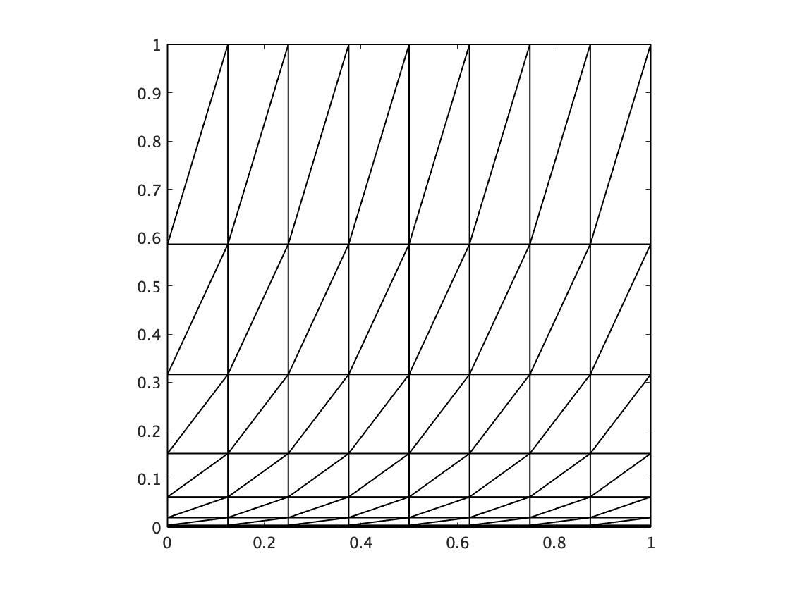
Figure 1: (Mesh I) Anisotropic mesh, $N=8$ and $\varepsilon=2.0$

Table 1: Mesh (I), mesh conditions, $\varepsilon=2.0$

$N$	$\#Np$	MinAngle	MaxAngle	DisSov
4	144	8.50	2.00	1.04199
8	544	1.63e+01	2.00	7.63521e-01
16	2,112	3.21e+01	2.00	5.95764e-01
32	8,320	6.41e+01	2.00	5.00244e-01
64	33,024	1.28e+02	2.00	4.20500e-01
128	131,584	2.56e+02	2.00	3.53564e-01

Table 2: Mesh (I), mesh conditions, $\varepsilon=4.0$

$N$	$\#Np$	MinAngle	MaxAngle	DisSov
4	144	1.28031e+02	2.00	1.68200
8	544	1.02400e+03	2.00	2.00000
16	2,112	8.19200e+03	2.00	2.37841
32	8,320	6.55360e+04	2.00	2.82843
64	33,024	5.24288e+05	2.00	3.36359
128	131,584	4.19430e+06	2.00	4.00000

The theoretical results of the modified CR finite element method for an anisotropic mesh partition are numerically verified and presented in Tables 3, 4, and 5. When $\epsilon=4.0$, condition (3.18) is not satisfied. However, the numerical result indicates an optimal convergence rate as meshes become finer.

Table 3: Mesh (I), Example 1, $\varepsilon=1.0$

$N$	$h$	$Err(V_{h})$	$r$	$Err(L^{2})$	$r$	$Err(Q_{h})$	$r$
4	3.54e-01	9.30891e-01		5.57356e-01		2.77363e-01
8	1.77e-01	5.06405e-01	0.88	1.63541e-01	1.77	1.39270e-01	0.99
16	8.84e-02	2.59214e-01	0.97	4.33267e-02	1.92	6.97005e-02	1.00
32	4.42e-02	1.30439e-01	0.99	1.10344e-02	1.97	3.48582e-02	1.00
64	2.21e-02	6.53276e-02	1.00	2.77257e-03	1.99	1.74301e-02	1.00
128	1.10e-02	3.26775e-02	1.00	6.93973e-04	2.00	8.71516e-03	1.00

Table 4: Mesh (I), Example 1, $\varepsilon=2.0$

$N$	$h$	$Err(V_{h})$	$r$	$Err(L^{2})$	$r$	$Err(Q_{h})$	$r$
4	5.04e-01	1.04386		7.54616e-01		2.28331e-01
8	2.66e-01	6.00986e-01	0.80	2.50020e-01	1.59	1.13984e-01	1.00
16	1.36e-01	3.14178e-01	0.94	7.08474e-02	1.82	5.69444e-02	1.00
32	6.90e-02	1.59284e-01	0.98	1.85985e-02	1.93	2.84658e-02	1.00
64	3.47e-02	7.99483e-02	0.99	4.71970e-03	1.98	1.42321e-02	1.00
128	1.74e-02	4.00138e-02	1.00	1.18479e-03	1.99	7.11597e-03	1.00

Table 5: Mesh (I), Example 1, $\varepsilon=4.0$

$N$	$h$	$Err(V_{h})$	$r$	$Err(L^{2})$	$r$	$Err(Q_{h})$	$r$
4	7.28e-01	1.13521		9.15578e-01		3.45283e-01
8	4.32e-01	8.34160e-01	0.44	5.29158e-01	0.79	1.65246e-01	1.06
16	2.36e-01	4.72051e-01	0.82	1.80204e-01	1.55	8.17474e-02	1.02
32	1.23e-01	2.47274e-01	0.93	5.25128e-02	1.78	4.07539e-02	1.00
64	6.30e-02	1.25537e-01	0.98	1.39353e-02	1.91	2.03619e-02	1.00
128	3.19e-02	6.30344e-02	0.99	3.54646e-03	1.97	1.01790430e-02	1.00

5.2 Example 2

The second example demonstrates the robustness of the proposed scheme for large irrotational body forces on anisotropic mesh partitions. We consider the numerical example inspired by LinMer16 ; QuiPie20 ; YanHeZha22 . The exact solution $(u,p)$ in (5.1) with velocity and pressure is given by

$$\displaystyle\begin{pmatrix}u_{1}\\ u_{2}\end{pmatrix} =\begin{pmatrix}-\left(x_{2}-\frac{1}{2}\right)\\ x_{1}-\frac{1}{2}\end{pmatrix},$$

$$p =\left(x_{1}-\frac{1}{2}\right)^{2}+\left(x_{2}-\frac{1}{2}\right)^{2}-\frac{1}{6}+10^{5}(1-x_{2})^{3}-\frac{10^{5}}{4}.$$

Note that $\int_{\Omega}pdx=0$. Setting $\nu=1$, the force is exactly irrotational, i.e.,

$$\displaystyle\begin{pmatrix}f_{1}\\ f_{2}\end{pmatrix} =\begin{pmatrix}0\\ -3\times 10^{5}(1-x_{2})^{2}\end{pmatrix}.$$

Let $N\in\{4,8,16,32,64,128\}$ be the division number of each side of the bottom and the height edges of $\Omega$. We consider the following mesh partitions. Let $(x_{1}^{i},x_{2}^{i})^{T}$ be grip points of triangulations $\mathbb{T}_{h}$ defined as follows. Let $i\in\mathbb{N}$.

(Mesh II) Anisotropic mesh which comes from CheLiuQia10 (Fig. 2)

$$\displaystyle x_{1}^{i}:=\frac{1}{2}\left(1-\cos\left(\frac{i\pi}{N}\right)\right),\quad x_{2}^{i}:=\frac{1}{2}\left(1-\cos\left(\frac{i\pi}{N}\right)\right),\quad i\in\{0:N\}.$$

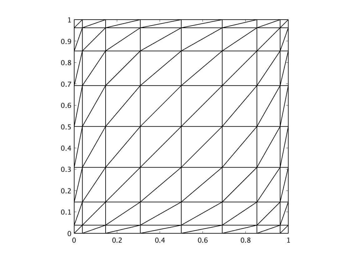
Figure 2: (Mesh II) Anisotropic mesh, $N=8$

Table 6: Mesh (II), mesh conditions

$N$	$\#Np$	MinAngle	MaxAngle	DisSov
4	144	5.65685	2.00	1.00000
8	544	1.04525e+01	2.00	7.94187e-01
16	2,112	2.05033e+01	2.00	6.66204e-01
32	8,320	4.08092e+01	2.00	5.59870e-01
64	33,024	8.15201e+01	2.00	4.70722e-01
128	131,584	1.62991e+02	2.00	3.95813e-01

Tables 7, and 8 numerically verifies the theoretical results of the modified CR finite element method for an anisotropic mesh partition and confirm the robustness towards irrotational body forces on anisotropic mesh partitions.

Table 7: Mesh (I), Example 2, $\varepsilon=1.0$

$N$	$h$	$Err(V_{h})$	$r$	$Err(L^{2})$	$r$	$Err(Q_{h})$	$r$
4	3.54e-01	9.09364e-07		5.47195e-07		2.77362e-01
8	1.77e-01	2.66354e-06	-	1.24705e-06	-	1.39270e-01	0.99
16	8.84e-02	1.97022e-06	-	1.24596e-06	-	6.97007e-02	1.00
32	4.42e-02	1.73889e-06	-	9.04173e-07	-	3.48583e-02	1.00
64	2.21e-02	1.26862e-06	-	5.57509e-07	-	1.74301e-02	1.00
128	1.10e-02	1.43621e-06	-	8.86565e-07	-	8.71518e-03	1.00

Table 8: Mesh (II), Example 2

$N$	$h$	$Err(V_{h})$	$r$	$Err(L^{2})$	$r$	$Err(Q_{h})$	$r$
4	5.00e-01	2.98226e-06		1.08150e-06		2.87956e-01
8	2.71e-01	2.81107e-06	-	1.70024e-06	-	1.49758e-01	0.94
16	1.38e-01	4.52069e-06	-	2.75827e-06	-	7.54093e-02	0.99
32	6.93e-02	2.36901e-06	-	9.65821e-07	-	3.77670e-02	1.00
64	3.47e-02	2.73752e-06	-	1.11624e-06	-	1.88912e-02	1.00
128	1.74e-02	2.08281e-06	-	8.56957e-07	-	9.44656e-03	1.00

6 Concluding remarks

We developed the modified CR finite element method to the rotation form of the stationary incompressible Navier–Stokes equation on the anisotropic mesh partitions. The proposed method achieves pressure-independent velocity error estimates. The numerical examples verify the theoretical results. In the future, we will extend the proposed approach to the time-dependent Navier–Stokes problems and high Reynolds number flows.

Moreover, in numerical example 2, we had imposed the inhomogeneous Dirichlet boundary condition on the simply connected domain although we did not study the case. In general, we assume that $\Omega\subset\mathbb{R}^{d}$, $d\in\{2,3\}$, is an open, bounded, connected but multiply-connected, and its boundary $\Gamma$ is Lipschitz-continuous for analysis. We consider $\Gamma_{0}$ as the exterior boundary of $\Omega$, and the other components of $\Gamma$ using $\Gamma_{i}$, $1\leq i\leq M$. For $M\in\mathbb{N}$, we assume that

$$\displaystyle\int_{\Gamma_{i}}g\cdot nds=0,\quad 0\leq i\leq M,$$ (6.1)

where $n=(n_{1},\ldots,n_{d})^{T}$ denotes the unit outward normal to $\Gamma_{i}$, $0\leq i\leq M$. (6.1) is called the stringent outflow condition. In addition, from the divergence formula,

$$\displaystyle\int_{\Gamma}g\cdot nds=\int_{\Omega}\mathop{\mathrm{div}}udx=0.$$ (6.2)

This is called the general outflow condition. We plan to extend the proposed approach to problems imposed by other boundary conditions, including inhomogeneous Dirichlet boundary conditions.

References

- (1) Apel, Th., Nicaise, S., Schöberl, J.: Crouzeix–Raviart type finite elements on anisotropic meshes. Numer. Math. 89, 193-223 (2001)
- (2) Boffi, D., Brezzi, F., Fortin, M.: Mixed Finite Element Methods and Applications. Springer Verlag, New York (2013)
- (3) Brandts, J., Korotov, S., Kíek, M.: On the equivalence of regularity criteria for triangular and tetrahedral finite element partitions. Comput. Math, Appl. 55, 2227–2233 (2008)
- (4) Chen, S., Liu, M., Qiao, Z.: An anisotropic nonconforming element for fourth order elliptic singular perturbation problem. International Journal of Numerical Analysis and Modeling 7 (4), 766-784 (2010)
- (5) Dauge, M.: Elliptic boundary value problems on corner domains. vol. 1341 of Lecture Notes in Mathematics, Springer–Verlag, Berlin, (1988)
- (6) Ern, A., Guermond, J.L.: Theory and Practice of Finite Elements. Springer Verlag, New York (2004)
- (7) Ern, A., Guermond, J.L.: Finite Elements I: Galerkin Approximation, Elliptic and Mixed PDEs. Springer Verlag, New York (2021)
- (8) Ern, A., Guermond, J.L.: Finite Elements II: Galerkin Approximation, Elliptic and Mixed PDEs. Springer Verlag, New York (2021)
- (9) Ern, A., Guermond, J.L.: Finite Elements III: First-Order and Time-Dependent PDEs. Springer Verlag, New York (2021)
- (10) Girault, V., Raviart, P.A.: Finite Element Methods for Navier-Stokes Equations. Springer-Verlag, (1986)
- (11) Grisvard, P.: Elliptic Problems in Nonsmooth Domains. SIAM, (2011)
- (12) Ishizaka, H.: Anisotropic Raviart–Thomas interpolation error estimates using a new geometric parameter. Calcolo 59 (4), (2022)
- (13) Ishizaka, H.: Morley finite element analysis for fourth-order elliptic equations under a semi-regular mesh condition. submitted, (2023)
- (14) Ishizaka, H., Kobayashi, K., Tsuchiya, T.: Anisotropic interpolation error estimates using a new geometric parameter. Jpn. J. Ind. Appl. Math., 40 (1), 475-512 (2023)
- (15) John, V.: Finite element methods for incompressible flow problems, Springer, (2016)
- (16) John, V., Linke, A., Merdon, C., Neilan, M., Rebholz, L.G.: On the divergence constraint in mixed finite element methods for imcompressible flows. SIAM Rev. 59 (3), 492–544 (2017)
- (17) Lederer, P., Linke, A., Merdon, C., Schöberl, J.: Divergence-free reconstruction operators for pressure-robust Stokes discretization with continuous pressure finite elements. SIAM J. Numer. Anal. 55 (5), 1291–1314 (2017)
- (18) Linke, A.: On the role of the Helmholtz decomposition in mixed methods for incompressible flows and a new variational crime. Comput. Methods Anall. Mech. Engrg. 268, 782-800 (2014)
- (19) Linke, A., Matthies, G., Tobiska, L.: Robust arbitrary order mixed nite element methods for the incompressible Stokes equations with pressure-independent velocity errors. ESIAM: M2AN 50, 289–309 (2016)
- (20) Linke, A., Merdon, C.: Pressure-robustness and discrete Helmholtz projectors in mixed finite element methods for the incompressible Navier–Stokes equations. Comput. Methods Appl. Mech. Engrg. 311, 304-326 (2016)
- (21) Linke, A., Merdon, C.: On velocity errors due to irrotational forces in the Navier–Stokes momentum balance. Journal of Computational Physics 313, 654-661 (2016)
- (22) Di Pietro, D.A., Ern, A.: Mathematical Aspects of Discontinuous Galerkin Methods. Springer Verlag, (2012)
- (23) Quiroz, D.C., Di Pietro, D.A.: A Hybrid High-Order method for the incompressible Navier–Stokes problem robust for large irrotational body forces. Comput. Math. Appl. 79, 2655-2677 (2020)
- (24) Sohr, H.: The Navier-Stokes Equations: An Elementary Functional Analytic Approach. Birkhuser, Boston, Basel, Berlin, (2001)
- (25) Temam, R.: Navier-Stokes Equations, Theory and Numerical Analysis, Third, (revised) edition. North-Holland, Amsterdam, (2001)
- (26) Wihler, T. P., Rivière B.: Discontinuous Galerkin Methods for Second-Order Elliptic PDE with Low-Regularity Solutions. J. Sci. Comput. 46, 151-165 (2011)
- (27) Yang, D., He, Y., Zhang, Y.: Analysis and computation of a pressure-robust method for the rotation form of the incompressible Navier–Stokes equations with high-order finite elements. Computers & Mathematics with Applications 112 (15), 1-22 (2022)