Bifurcations of mode-locked periodic orbits in three-dimensional maps

Abstract

In this paper, we report the bifurcations of mode-locked periodic orbits occurring in maps of three or higher dimensions. The ‘torus’ is represented by a closed loop in discrete time, which contains stable and unstable cycles of the same periodicity, and the unstable manifolds of the saddle. We investigate two types of ‘doubling’ of such loops: in (a) two disjoint loops are created and the iterates toggle between them, and in (b) the length of the closed invariant curve is doubled. Our work supports the conjecture of Gardini and Sushko, which says that the type of bifurcation depends on the sign of the third eigenvalue. We also report the situation arising out of Neimark-Sacker bifurcation of the stable and saddle cycles, which creates cyclic closed invariant curves. We show interesting types of saddle-node connection structures, which emerge for parameter values where the stable fixed point has bifurcated but the saddle has not, and vice versa.

I Introduction

Mode-locked periodic orbits occur when a dynamical system has two commensurate frequencies that are not harmonically related to each other. Such cycles always occur as stable-unstable pairs, and are located on a closed invariant curve formed by the unstable manifolds of the saddle. Such closed invariant curves occurring in maps represent tori in continuous time. In this paper we investigate bifurcations of such ‘resonant tori’ in three-dimensional maps.

Much of the earlier work on the bifurcation of tori focused on ergodic tori or quasiperiodic orbits. The doubling of quasiperiodic orbits was first reported by Kaneko Kaneko83 and Arneodo et al. Spiegel83 in the dynamics of some three- and four-dimensional maps. Since then, such bifurcations have been reported in maps resulting from the discretization of continuous-time systems such as impulsive Goodwin’s oscillator Zhu21 , 3-dimensional Lotka-Volterra model Banerjee12 ; Gardini87 , vibro-impacting systems ding2004interaction , four coupled oscillators Ash95 , radiophysical systems Anish05 , etc. Sekikawa et al. demonstrated a sequence of length-doublings Seki01 ; Seki21 finally resulting in chaos.

Torus doubling critical point is a special point in the parameter space where the regions of occurrence of torus, doubled torus, and strange non-chaotic attractor meet. Such critical points were found in a nonlinear electronic circuit with quasiperiodic drive Seleznev2 . Scaling laws applicable in the vicinity of a critical point were obtained for a forced logistic map forcedlogistic .

For a better understanding on the bifurcations of invariant tori, iterative schemes for computation and continuation of two-dimensional stable and unstable manifolds of mode-locked orbits were proposed in Meiss06 ; Vitolo08 . In piecewise-smooth maps, the birth of a bilayered torus via border-collision bifurcation was reported in Zhu06 and bifurcation of such a torus via heteroclinic tangencies was discussed. Recently, a review on the dynamical consequences of torus doublings resulting in the formation of Shilnikov attractors were discussed in Gon21 .

After Grebogi, Ott and Yorke grebogi1983three showed that three-frequency quasiperiodicity can be stable over a parameter range, its occurrence, observed in the form of a torus in the discrete-time phase space, has been reported in many systems including symmetrical rigid tops nstoro6 , vibro-impacting systems Vibr15 , four coupled Chua’s circuits zhong1998torus , a simple autonomous system kuznetsov2016simplest , and a ladder of four coupled van der Pol oscillators Kom16 .

The merger and disappearance of a stable and an unstable closed invariant curves was found to be responsible for the creation of strange nonchaotic attractors Hammel94 ; FEU95 ; SNAbook06 . Behaviors close to tori-collision terminal points were studied in kuznetsov2000critical .

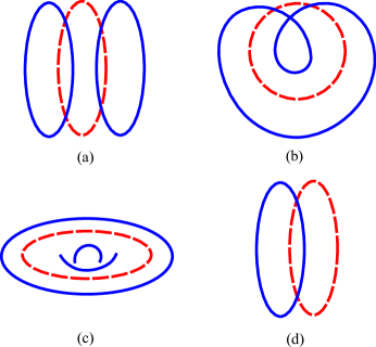
Figure 1: The four types of bifurcations of a quasiperiodic orbit Banerjee12 . Unstable objects are shown with red dashed lines and stable objects are marked in blue.

These observations have been summarized in Banerjee12 , by showing that a stable quasiperiodic orbit can bifurcate in four possible ways. These are illustrated in Fig. 1. Fig. 1(a) and (b) show two ways of ‘doubling’: in (a) two disjoint loops are created and the iterates toggle between them, and in (b) the length of the closed invariant curve is doubled. The bifurcation shown in Fig. 1(c) leads to a torus in discrete time which represents three-frequency quasiperiodicity. Fig. 1(d) shows a situation where a stable and an unstable tori merge and disappear (or are created if the parameter is varied in the opposite direction). Banerjee et al. explained these bifurcations based on the method of ‘second Poincaré section’ Banerjee12 .

The above lines of work concern bifurcations of quasiperiodic orbits. However, mode-locked periodic orbits represent a generic case. Such orbits possess rational rotational numbers and appear as shrimp shaped regions in two-dimensional parameter space Ga94 that cover a larger range of parameters than the quasiperiodic orbit. Therefore, in this paper we explore the ways in which␣‌mode-locked periodic orbits may bifurcate.

Although much research has been done on the doubling of quasiperiodic orbits, much less research attention has been devoted to the doubling of resonant tori or mode-locked periodic orbits. Gardini and Sushko Gardini12 proposed a conjecture regarding the conditions for different types of doubling bifurcations of closed invariant curves related to mode-locked periodic orbits. However, to date these have not been tested using systems that exhibit these bifurcations. In this paper we fill that gap and validate their conjecture.

We also explore the birth of a third frequency in a mode-locked periodic orbit, which results in the occurrence of more than two closed invariant curves in the phase space and the iterates cyclically move among them.

Both types of torus doubling are related to the occurrence of period doubling bifurcation and the birth of multiple loops is related to the occurrence of a Neimark-Sacker bifurcation in a fixed point. Since a saddle cycle as well as a stable cycle occur on the closed invariant curve, an interesting situation emerges: it is possible that one of them undergoes a bifurcation but the other does not. Such situations lead to atypical structures of the closed invariant curve, which are also reported in this paper.

The paper is organized as follows: In §II, we recapitulate the conjecture and discuss the mechanism behind the doubling of mode-locked orbits in three-dimensional maps. In §III, we give an example of the doubling phenomenon of a mode-locked periodic orbit in a three-dimensional smooth map where two disjoint loops are formed. In §IV, we provide example of the case where the length of manifold doubles and they lie on a non-orientable Möbius strip. In §VII, collision of two closed invariant curves formed out of a saddle-node connection and a saddle-saddle connection is discussed. §VIII presents the conclusions and future research questions arising out of this paper.

II Qualitative theory of doubling of mode-locked orbit

Closed invariant curves are born through Neimark-Sacker bifurcation of a stable fixed point. This can lead to a few scenarios:

1. A supercritical Neimark-Sacker bifurcation leading to the formation of a stable closed invariant curve.

   1. There are a dense set of points on the curve, which implies an irrational frequency ratio. This leads to the formation of a quasiperiodic orbit.

   2. There are a finite number of stable and saddle points and the invariant closed curve is composed of a union of these points and the unstable manifolds of the saddle points. This leads to the formation of a mode-locked periodic orbit.

2. A subcritical Neimark-Sacker bifurcation leading to an unstable closed invariant curve.

   1. The unstable closed invariant curve may be a quasiperiodic orbit;

   2. The unstable closed invariant curve may be a mode-locked periodic orbit.

In this paper we consider the bifurcations of a closed invariant curve related to Case 1(b).

Let us consider a three-dimensional map with a stable cycle (say $C^{N}$) and saddle cycle (say $C^{S}$). The union of these points and the unstable manifolds of the saddle cycles form the closed invariant curve (see Fig. 2). Let us denote the eigenvalues of the stable periodic orbit as $\lambda_{i}^{N}$, $i=1,2,3$ and the eigenvalues of the saddle periodic orbit as $\lambda_{i}^{S}$, $i=1,2,3$.

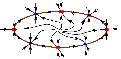
Figure 2: Schematic structure of a closed invariant curve for a mode-locked periodic orbit. The stable cycle is marked by blue triangles and the saddles by red rectangles. The directions associated with eigenvalues 1, 2 and 3 of the stable cycle are shown for one of the points.

In order for the closed invariant curve to exist, one of the three eigenvalues must be positive. Let the positive eigenvalues be denoted by $\lambda_{1}^{N},\lambda_{1}^{S}$ for the node and saddle periodic points, respectively. The corresponding stable manifolds of the nodes and the unstable manifolds of the saddles form the saddle-node connections on the closed invariant curve.

Following Gardini12 , let us first consider the case of doubling of the closed invariant curve. In order for a doubling to occur, there must be a flip bifurcation, i.e., one of the eigenvalues should pass through $-1$. Let this eigenvalue be denoted as $\lambda_{2}^{N}$ for the node and as $\lambda_{2}^{S}$ for the saddle. These eigenvalues, associated with the saddle and the node, need not pass through $-1$ at the same parameter value. Indeed, the saddle and the node can undergo flip bifurcation at different parameter values. We will see this in two explicit examples considered later in this paper.

Consider a situation where both the saddle $C^{S}$ and the node $C^{N}$ have undergone flip bifurcation (see Fig. 3). A doubled stable orbit (say $C^{2N}$) has emanated from $C^{N}$, which has turned into a flip-saddle with one unstable direction. A similar scenario occurs with the saddle periodic point $C^{S}$, which doubles by making another of its branches unstable (two independent unstable directions). Two saddle points (say $C^{2S}$) emanate on both sides of the previous saddle ($C^{S}$).

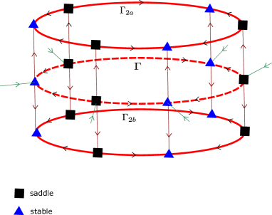
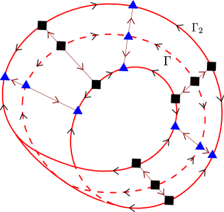
(a)                                                           (b)

Figure 3: In (a), the doubling bifurcation related to the positive third eigenvalue leading to disjoint loops. In (b), the doubling bifurcation related to negative third eigenvalue and the mode locked periodic orbit lies on the surface of a Möbius strip.

Two distinctly different stable behaviors can result from this bifurcation. Gardini and Sushko Gardini12 conjectured that the shape of the resulting manifold is determined by the third eigenvalue $\lambda_{3}^{N},\lambda_{3}^{S}$. The sign of the third eigenvalue classifies the bifurcation into two types.

II.1 Positive third eigenvalue ($\lambda_{3}^{N}>0,\lambda_{3}^{S}>0$)

If the third eigenvalue associated is positive, then the trajectories will be converging on one side of the manifold and will give a geometric structure like Fig. 3(a). This leads to the formation of two disjoint cycles $\Gamma_{2a},\Gamma_{2b}$. We note that the two disjoint cycles are cyclically invariant, i.e., the trajectory on the periodic orbits toggle between the upper cycle $\Gamma_{2a}$ and the lower cycle $\Gamma_{2b}$. The two disjoint closed loops are invariant in the sense that they act as a single loop for the second iterate of the map.

The two attracting disjoint cycles bound a strip or a manifold whose shape is topologically a cylinder. The manifold (topological cylinder) consists of the unstable closed cycle $\Gamma$ and the two stable disjoint cycles $\Gamma_{2a}$, and $\Gamma_{2b}$. The cylinder manifold is orientable. Each of the node and saddle periodic points ($C^{N},C^{S},C^{2N},C^{2S}$) have three independent eigen-directions, which are represented in Fig. 3 with different colours.

II.2 Negative third eigenvalue ($\lambda_{3}^{N}<0,\lambda_{3}^{S}<0$)

If the third eigenvalue is negative, the shape of the invariant set is a Möbius strip (a non-orientable manifold). The boundary of the Möbius strip constitutes the saddle-node connection of the doubled saddle and node mode-locked periodic orbits. This is qualitatively shown in Fig. 3(a).

We now illustrate the above bifurcations with a few examples.

III Example: Disjoint two-loop mode-locked orbit

In this section we consider the Mira map studied in Kara21 , which is a three-dimensional map given by

$$x^{\prime} =y,$$ (1)

$$y^{\prime} =z,$$

$$z^{\prime} =Bx+Cy+Az-y^{2},$$

The Jacobian of the map (1) is

$$J=\begin{bmatrix}0&1&0\\ 0&0&1\\ B&C-2y&A\end{bmatrix},$$ (2)

whose determinant is det$(J)=B$. For $B<0$, the map is orientation-reversing everywhere, and for $B>0$, the map is orientation-preserving everywhere. We have observed disjoint two-loop mode-locked periodic orbit in the orientation-reversing regime. In Kom16 , authors have mentioned that such disjoint doublings of quasiperiodic orbit can be found in orientation-preserving systems as well but in higher dimensional systems of dimensions greater than or equal to four.

From the one-parameter bifurcation diagram with the variation of parameter $B$, see Fig. 4(a), we observe that a fixed point undergoes a Hopf bifurcation to a quasiperiodic orbit and then through a saddle-node bifurcation, a mode-locked period-five orbit is formed. It then doubles to a period-10 mode-locked orbit. With further increase in the parameter $B$, we observe subsequent doublings of mode-locked orbit, after which it transits to chaos.

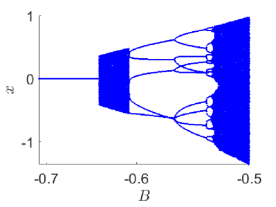
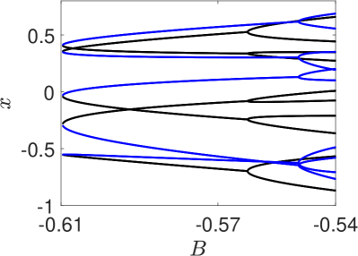
(a)                                   (b)

Figure 4: (a) One-parameter bifurcation diagram of $x$ vs $B$. The parameters are $A=-2.269,C=-2.1$. At $B=-0.58$, we observe a period-5 mode-locked orbit. At $B=-0.54$, we observe a period-10 mode-locked orbit. When $B$ is further increased, it undergoes subsequent period-doubling bifurcations leading to chaos. (b) One-parameter bifurcation diagram showing both the saddle (black) and stable (blue) periodic points.

The doubling of the mode-locked orbit can be better understood when we continue the saddle and stable mode-locked periodic orbits with respect to the parameter $B$. We have used the multidimensional Newton-Raphson method to locate the saddle cycle. Fig. 4(b) shows that the saddle doubles first, followed by the doubling of the node. The computation of the eigenvalues over the same parameter range of $a$ (see Fig. 5) reveals that, as the parameter $B$ increases, the second eigenvalue reaches $-1$ at $B=-0.5627$. In Fig. 5(b), we see that the second eigenvalue of the node reaches $-1$ at $B=-0.55$ and hence the stable period-five orbit bifurcates to a period-ten orbit.

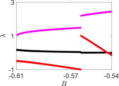
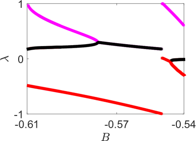
(a)                                     (b)

Figure 5: Continuation of the eigenvalues as the parameter $B$ is varied: (a) for the saddle cycle and (b) for the stable cycle. Three eigenvalues are differentiated by different colours: eigenvalue $\lambda_{1}$ is denoted by magenta, $\lambda_{2}$ by red, and $\lambda_{3}$ by black.

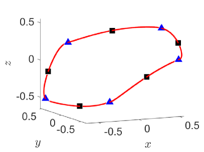
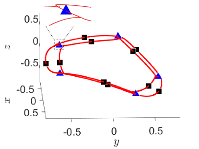
(a)                                     (b)
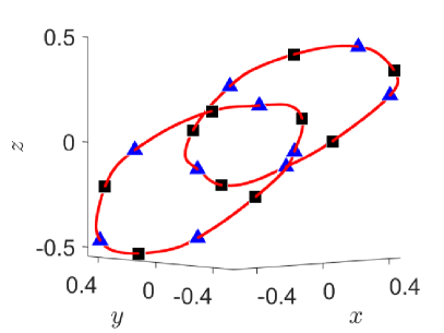
(c)

Figure 6: (a) The closed invariant curve formed by the unstable manifolds (in red) of the saddle period-5 periodic orbit at $B=-0.58$. The stable mode-locked period-5 orbit is denoted by blue triangles and the saddle period-5 orbit is denoted by black squares. (b) The structure of the closed invariant curve for $B=-0.555$, when the saddle has doubled but the stable cycle has not yet doubled. The zoomed portion shows the connection through the stable fixed point. (c) At $B=-0.54$, two disjoint loops are formed by the unstable manifolds of two disjoint yet cyclic saddle period-10 mode-locked orbits. The other parameters are $A=-2.269$ and $C=-2.1$.

At $B=-0.58$, a stable period-5 mode-locked orbit exists along with a period-5 saddle. We compute the unstable manifolds of the saddle cycle using the method of fundamental domains MuMcSi21 , which form a saddle-node connection. The resulting invariant closed curve is shown in Fig. 6(a).

As we increase the parameter $B$, a stage is reached where the saddle has doubled but the stable periodic orbit has not. At $B=-0.555$, the saddle period-10 orbit coexists with a stable period-five orbit. The manifolds of the saddle point are shown in Fig. 6(b). We notice a complex structure in which two loops have formed, but these are joined by branches that connect with the stable period-5 orbit.

Next, we consider a parameter where both the saddle and stable mode-locked periodic orbit have doubled. At $B=-0.54$, we see a mode locked period-10 orbit and the unstable manifolds of the period-doubled saddle cycle shows two disjoint loops (Fig. 6(b)).

Note that this disjoint mode-locked periodic orbit does not imply bistability, rather the periodic points of the disjoint loops are cyclically visited. The second iterate of the map shows a single loop.

The eigenvalues of the saddle and stable periodic points before the bifurcation are shown in Table 1. We note that before the torus doubling bifurcation, $\lambda_{1}$ is positive, $\lambda_{2}$ is negative (which subsequently crosses $-1$), and $\lambda_{3}$ is positive. Thus, our observation supports the conjecture by Gardini and Sushko.

Type	$\lambda_{1}$	$\lambda_{2}$	$\lambda_{3}$
Stable	0.3550	-0.7131	0.2593
Saddle	1.3963	-0.7878	0.0597

Table 1: The eigenvalues of stable and saddle period-5 cycles for $B=-0.58$.

IV Example: Length doubled mode-locked orbit

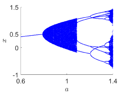
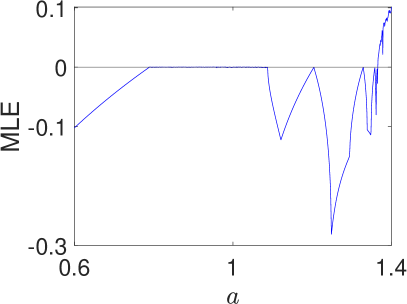
(a)                                     (b)

Figure 7: In (a), a one-parameter bifurcation diagram of the generalised Hénon map upon varying parameter $a$. In (b), plot of the maximal Lyapunov exponent in the same parameter range. The other parameter is fixed as $b=0.1$.

We consider the three-dimensional generalised Hénon map Richter02 given by

$$x^{\prime} =a-y^{2}-bz,$$ (3)

$$y^{\prime} =x,$$

$$z^{\prime} =y,$$

where $a,b$ are the parameters. Fig. 7(a) shows a one-parameter bifurcation diagram for this system considering $a$ as the parameter, with $b$ fixed at 0.1. A period-1 orbit bifurcates to a quasiperiodic orbit at $a\approx 0.78$ as evidenced by the maximal Lyapunov exponent being zero (Fig. 7(b)). A stable period-4 orbit emerges at $a\approx 1.08$.

Fig. 8 shows the saddle period-4 orbit with black squares and the stable period-4 orbit with blue triangles. We observe that they indeed form a saddle-node connection forming a single loop. Thus, the orbit existing for $a=1.2$ is a mode-locked period-4 cycle.

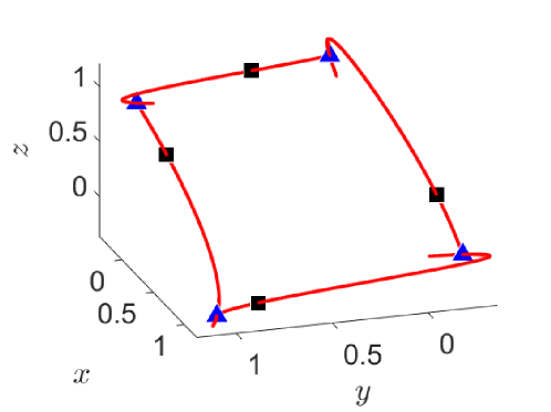
Figure 8: Saddle-node connection of stable and saddle mode locked period-4 orbit for $a=1.2,b=0.1$.

We now investigate what happens to this cycle as the parameter $a$ is varied. A one-parameter bifurcation diagram obtained using a continuation algorithm for both the saddle and stable cycles, is shown in Fig. 9. It shows that the two orbits bifurcate at different parameter values. There is a range, approximately [1.205, 1.29], where the stable orbit has bifurcated but the saddle has not.

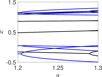
Figure 9: Variation of the saddle (black) and stable (blue) periodic orbits with parameter $a$, where $b$ is fixed at 0.1.

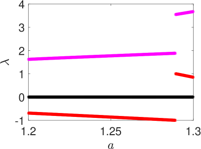
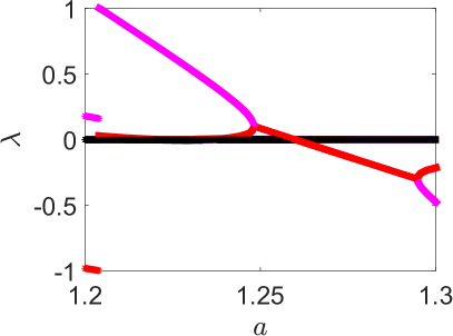
(a)                                     (b)

Figure 10: Variation of the eigenvalue of the saddle cycle (a) and the stable cycle (b) with parameter $a$. The parameter $b$ is fixed at 0.1. The three eigenvalues are shown with different colours: $\lambda_{1}$ is denoted by magenta, $\lambda_{2}$ by red, and $\lambda_{3}$ by black.

Continuation of the eigenvalues of both the saddle and stable mode-locked periodic orbits as a parameter varies, is presented in Fig. 10. Fig. 10(a) and (b) show that with increase of the parameter, at $a=1.204$, $\lambda_{2}$ reaches $-1$, which leads to the period doubling.

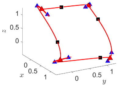
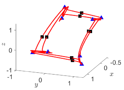
(a)                                     (b)

Figure 11: (a) The situation at $a=1.25$ and $b=0.1$ where the stable period-4 cycle has already doubled but the saddle cycle has not. The stable period-8 cycle (shown as blue triangles) has emerged through a flip bifurcation of the period-4 cycle (marked in red triangles, now a saddle), and the saddle periodic orbit marked by black squares. (b) Saddle-node connection of stable and saddle mode locked period-eight orbit for $a=1.3,b=0.1$. The red curve denotes the unstable manifold making a loop with double length.

When the stable cycle has already doubled but the saddle one has not (Fig. 11(a)), the unstable manifolds of the saddle points (red line) form a single closed loop structure connecting all the points. Branches emerge from the saddle period-4 cycle (which was earlier the node) to connect the stable period-8 points.

We next consider a parameter value $a=1.3$, $b=0.1$, at which the saddle and stable period-eight orbits coexist. The period-eight orbit cyclically visits each of its points. Considering both branches of the unstable manifold, we observe that the closed invariant curve winds around twice and its length has doubled, see Fig. 11(b).

Type	$\lambda_{1}$	$\lambda_{2}$	$\lambda_{3}$
Stable	0.1795	-0.9813	-0.0006
Saddle	1.6217	-0.6890	-0.0001

Table 2: The eigenvalues of stable and saddle cycles for $a=1.2,b=0.1$, i.e., before the bifurcation

For $a=1.2,b=0.1$, the eigenvalues of the stable and saddle period-four orbits are given in Table 2. It shows that before the bifurcation, $\lambda_{1}^{N}$ and $\lambda_{1}^{S}$ are positive and $\lambda_{2}^{N}$ and $\lambda_{2}^{S}$ are negative. As the parameter is varied, $\lambda_{2}^{N}$ reaches $-1$ first, followed by $\lambda_{2}^{S}$. The third eigenvalue is negative. Under this condition, Gardini12 conjectured that the shape of the manifold should be a Möbius strip and a length-doubling biurcation would occur. Our numerical results support the conjecture.

V From mode-locked orbits to cyclic invariant closed curves

It is known that when a third frequency is born from a quasiperiodic orbit, it creates a torus in discrete time. In this section we present the mechanisms of generation of a third frequency from a mode-locked periodic orbit. We find that it can result in two types of orbits. The resulting orbit can be a collection of quasiperiodic loops located on a torus in the discrete-time phase space (schematically shown in Fig. 12), and the iterates visit them cyclically. The resulting orbit can also be a mode-locked periodic orbit where the points are connected by cyclic closed invariant curves.

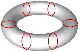
Figure 12: Multiple loops located on a torus

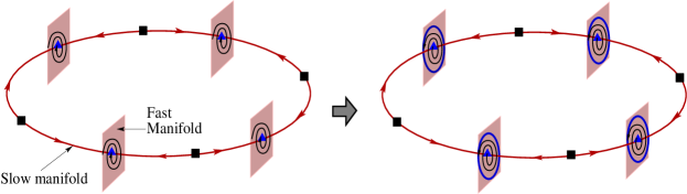
(a)                                                       (b)

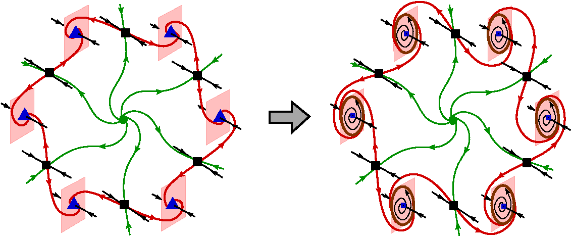
(c)                                                        (d)

Figure 13: Schematic representations of the two mechanisms of creation of multiple loops through Neimark-Sacker bifurcation. The blue triangles represent the foci, the black squares represent the saddles.

How can such structures be created? Since the birth of a third frequency is caused by a Neimark-Sacker bifurcation, i.e., a pair of complex conjugate eigenvalues exiting the unit circle, the starting point in such a transition has to be a closed invariant curve created out of a saddle-focus connection. If a closed invariant curve is composed of a saddle-node connection as shown in Fig. 2, with the change of a parameter a pair of real eigenvalues have to turn complex conjugate, thus creating a saddle-focus connection.

The saddle-focus connection can be of two types. The unstable manifold of the saddle cycle can either connect with the one-dimensional stable manifold associated with the real eigenvalue or with the two-dimensional stable manifold associated with the complex conjugate eigenvalues of the focus. It depends on the rate of convergence along the manifolds. If the 1D manifold associated with the real eigenvalue is the slow one, the unstable manifold connects with it (Fig. 13(a)). An example of this situation was presented in de2011local . If the 2D manifold is the slow one, the unstable manifold of the saddle spirals into the node along this manifold (Fig. 13(c)).

The Neimark-Sacker bifurcation occurring in these two types of saddle-node connection are shown in Fig. 13. In both cases, if there are $n$ points in the stable cycle, $n$ cyclic closed invariant curves are created.

In the first case, the repelling focus creates a loop around it and the saddle-focus connection through the 1D manifold remains intact (see Fig. 13(b)). In the second case, the unstable manifolds of the saddle connect with the closed loops (see Fig. 13(d)). Note that in bifurcations of saddle-focus loops also, the saddle and the focus may bifurcate at different parameter values. Fig. 13 shows situations where the focus has bifurcated but the saddle has not.

We now give a few examples of the birth of cyclic closed invariant curves from saddle-focus connections in physical system models.

V.1 3D Lotka-Volterra model

In this section, we provide an explicit example of the situation schematically depicted in Fig. 13(c) and (d) using the three-dimensional Lotka-Volterra map Gardini87 given by

$$x^{\prime} =x+Rx(1-x-\alpha y-\beta z),$$ (4)

$$y^{\prime} =y+Ry(1-\beta x-y-\alpha z),$$

$$z^{\prime} =z+Rz(1-\alpha x-\beta y-z),$$

where $R,\alpha,\beta$ are the parameters of the system.

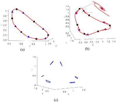
Figure 14: In (a), a saddle-node connection constituted by a saddle period-six orbit (marked by black squares) and a stable period-six orbit (marked by blue triangles) at $\beta=-0.59$. In (b), a saddle-focus connection constituted by a saddle period-six orbit (marked by black squares) and a stable period-six orbit (marked by blue triangles) at $\beta=-0.91$. The unstable manifold of each saddle periodic point is shown in red. In (c), six cyclic invariant closed curves are seen at $\beta=-1$ after the period-6 stable cycle has undergone a Neimark-Sacker bifurcation. The other parameters are $R=1,\alpha=1$.

For $R=1,\alpha=1,\beta=-0.59$, we observe a stable period-six orbit and a saddle period-six orbit. Considering the one-dimensional unstable manifold of each saddle periodic point, we observe a saddle-node connection in Fig. 14 (a). As $\beta$ is decreased to $-0.91$, two eigenvalues of the stable periodic point become complex conjugate, while the third one remains real, all of which have modulus less than one. The saddle cycle has two complex conjugate eigenvalues with modulus less than one and a real eigenvalue greater than one. Computation of the one-dimensional unstable manifolds of each saddle periodic point reveals formation of a saddle-focus connection (see Fig. 14(b)).

As the parameter $\beta$ is further decreased to $-1$, we observe that the period-6 stable cycle has undergone a Neimark-Sacker bifurcation and we can observe six cyclic closed invariant curves, see Fig. 14(c).

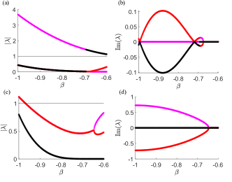
Figure 15: The variation of the eigenvalues with respect to the parameter $\beta$. (a) the modulus of the eigenvalues of the saddle, (b) the imaginary part of the eigenvalues of the saddle, (c) the modulus of the eigenvalues of the node, and (d) imaginary part of the eigenvalues of the node. The three eigenvalues are differentiated by three different colours (magenta, red, black). The other parameters are $R=1,\alpha=1$.

The variation of the eigenvalues of both saddle and stable periodic point with respect to the parameter $\beta$ is shown in Fig. 15. It shows that two eigenvalues of the stable cycle become complex at $\beta=-0.646$. The modulus crosses $1$ at $\beta=-0.968$. Subsequently we see the onset of a six cyclic closed invariant curve.

V.2 Three-dimensional border collision normal form

Piecewise smooth maps occur in many physical and engineering systems. It has been shown that, in the neighborhood of a border-crossing fixed point, such systems are aptly represented by a piecewise linear ‘normal form’ map BCNF99 . For three-dimensional piecewise smooth systems, the 3D border collision normal form is given by

$$X^{\prime}=F(X)=\begin{cases}A_{L}X+b\mu,&x\leq 0\\ A_{R}X+b\mu,&x>0,\\ \end{cases}$$ (5)

where $F:\mathbb{R}^{3}\rightarrow\mathbb{R}^{3},X=[x,y,z]^{T},b=[1,0,0]^{T}$ is a column vector, and $\mu\in\mathbb{R}$. The matrices $A_{L},A_{R}$ are defined by

$$A_{L}=\begin{bmatrix}\tau_{L}&1&0\\ -\sigma_{L}&0&1\\ \delta_{L}&0&0\end{bmatrix},\;\;\;\mbox{and}\;\;\;A_{R}=\begin{bmatrix}\tau_{R}&1&0\\ -\sigma_{R}&0&1\\ \delta_{R}&0&0\end{bmatrix}.$$ (6)

In Fig.16 (a), we observe a period-7 stable and saddle orbit marked by blue triangles and black squares respectively for $\delta_{R}=1.4$. A saddle-focus connection is observed. After increasing $\delta_{R}$ to $1.5$, seven cyclic closed invariant curves are observed. Continuation of the eigenvalues with variation of the parameter $\delta_{R}$ (Fig. 17) shows that for $\delta_{R}=1.4$, both the saddle cycle and the stable cycle have two complex conjugate eigenvalues and a real eigenvalue. At $\delta_{R}=1.455$, the complex conjugate eigenvalues cross the unit circle, and a 7-piece cyclic closed invariant curve is born.

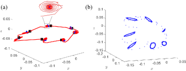
Figure 16: In (a), a saddle-focus connection at $\delta_{R}=1.4$ constituted by period-seven saddle orbit (marked by black squares) and stable period-seven orbit (marked by blue triangles). The unstable manifold of each saddle periodic point is shown in red. In (b), seven cyclic invariant closed curves are seen at $\delta_{R}=1.5$ after each stable periodic point has undergone a Neimark-Sacker bifurcation. The other parameters are $\tau_{R}=-0.5,\tau_{L}=0.74,\delta_{L}=0.73,\mu=0.01,\sigma_{L}=0.5,\sigma_{R}=1.1$.

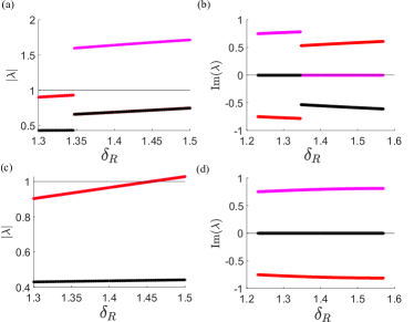
Figure 17: The variation of the eigenvalues with respect to the parameter $\delta_{R}$. In (a), the modulus of the eigenvalues of the saddle, (b) the imaginary part of the eigenvalues of the saddle, (c) the modulus of the eigenvalues of the node, and (d) imaginary part of the eigenvalues of the node. The three eigenvalues are differentiated by three different colours (magenta, red, black). The other parameters are set as $\tau_{R}=-0.5,\tau_{L}=0.74,\delta_{L}=0.73,\mu=0.01,\sigma_{L}=0.5,\sigma_{R}=1.1$.

VI Birth of three-frequency resonant torus

Let us consider the globally coupled three-dimensional map (7). A similar two-dimensional map has been studied in Zhu08 . The dynamical equations of the map are given by

$$x^{\prime} =f(x)+p\epsilon\Bigl{(}f(y)-f(x)\Bigr{)},$$ (7)

$$y^{\prime} =f(y)+(1-p)\epsilon\Bigl{(}f(x)-f(y)\Bigr{)},$$

$$z^{\prime} =x,$$

where

$$f(x)=x(1-x)(ax^{2}+(b^{2}-da)x+c),$$

and $p,\epsilon,a,b,c,d$ are parameters. A one-parameter bifurcation diagram with respect to parameter $a$ is presented in Fig 18.

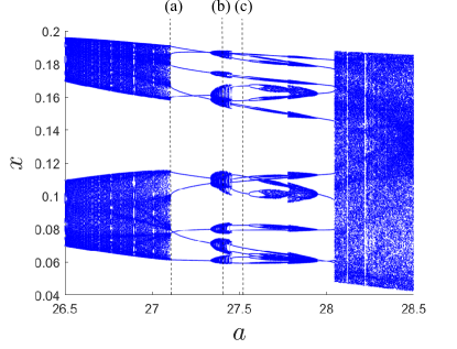
Figure 18: A one-parameter bifurcation diagram of (7) with respect to parameter $a$. The other parameters are fixed as $p=0.5,\epsilon=-1.4,b=1.688,c=3.5,d=0.85$. Three different parameter values are chosen as shown by dotted lines.

For $a<27.1107$, two disjoint cyclic quasiperiodic closed invariant curves exist. At $a=27.1107$, a period-$10$ orbit is born via a saddle-node bifurcation. Fig. 19(a) shows that the period-10 cycle occurs on two disjoint closed invariant curves connected by the one-dimensional unstable manifolds of a period-10 saddle cycle. When $a=27.408$, we observe each of the stable periodic points undergo a supercritical Neimark-Sacker bifurcation resulting in the formation of ten-disjoint cyclic closed loops, see Fig. 19(b).

The system develops two coexisting stable period-$20$ orbit for $a\in(27.461,27.6)$ (this is not shown to avoid the figure becoming messy). At $a=27.46$, ten disjoint cyclic closed loops are formed via a saddle-node bifurcation of a pair of stable and saddle period-$20$ orbits. Fig. 20 shows the bifurcation diagram in this parameter range. For clarity, we show the occurrence of saddle-node bifurcation for the cycles lying on a single loop (two stable period-2 and two saddle period-2 cycles). The concerned loop is shown in Fig. 19(d).

Similar saddle-node bifurcations occur in all 10 loops. At $a=27.5210$, there are 10 closed invariant curves formed through saddle-node connections. These are, in turn, located on two loops. The iterates toggle between the two bigger loops and move cyclically among the smaller loops. The resulting phase space is shown in Fig. 19(c). Note that the saddle and stable periodic orbits form cyclic disjoint loops connected via their one-dimensional unstable manifold. A zoomed-in version of one of the cyclic closed loops is shown in Fig. 19(d).

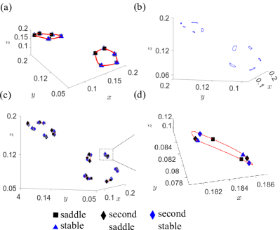
Figure 19: In (a), two disjoint cyclic closed invariant loops are observed comprising a stable period-10 orbit and a saddle period-10 orbit at $a=27.1107$. In (b), ten disjoint pieces of cyclic closed invariant curves are observed at $a=27.408$. In (c), ten disjoint pieces of closed invariant loops are observed comprising two stable period-$20$ orbits and two saddle period-$20$ orbits at $a=27.5210$. In (d), a magnified version of a single closed loop is shown.

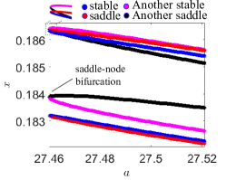
Figure 20: Continuation of periodic points lying on a single cyclic closed loop with respect to parameter $a$. Saddle-node bifurcation of a pair of two stable and two saddle periodic points lying on a single loop at $a=27.46$. Two stable and saddle points are marked in blue and red respectively. The other two coexisting stable and saddle points are marked in magenta and black respectively. The other parameters are fixed as $p=0.5,\epsilon=-1.4,b=1.688,c=3.5,d=0.85$.

VII Collision of saddle-node and saddle-saddle connections

It has been reported in Banerjee12 , that there can be situations where a stable torus and an unstable torus collide and disappear (see Fig. 1(d)). If the parameter is varied in the opposite direction, one can see the birth of a torus out of nothing. Such bifurcations, involving ergodic tori have been reported in power electronic systems.

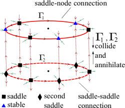
Figure 21: Collision of saddle-node connection $\Gamma_{1}$ with the saddle-saddle connection $\Gamma_{2}$. The saddle periodic orbits are denoted by black squares, another saddle periodic orbit with black diamond, and the stable periodic orbits are denoted by blue triangles.

The question is, can such a bifurcation involve resonant tori, i.e., mode-locked periodic orbits? In Fig. 21, we schematically show how such a collision between saddle-node connection $\Gamma_{1}$ and saddle-saddle connection $\Gamma_{2}$ can take place. The three eigendirections are shown in different colours and arrows.

As $\Gamma_{1}$ and $\Gamma_{2}$ approach each other as the parameter varies, they may collide and annihilate each other. If the parameter varies in the opposite direction, there is a sudden appearance of two closed invariant curves, one with a saddle-node connection and the other with a saddle-saddle connection. This is a topologically feasible scenario, but we have not yet found any physical system that exhibits this phenomenon.

VIII Conclusions

In this work, we have explored four scenarios related to the bifurcations of mode-locked periodic orbits and their associated closed invariant curves:

1. The birth of two disjoint closed invariant curves

2. The doubling of the length of the closed invariant curve

3. The birth of a few pieces of cyclic closed invariant curves

4. Merger and disappearance of two closed invariant curves, one involving a saddle-node connection and the other involving a saddle-saddle connection.

We have provided prototypical examples of three-dimensional maps in which bifurcation phenomena 1, 2, and 3 above can be observed. Through numerical simulations, we have validated the conjectures proposed in Gardini12 . In addition, we have shown the interesting structures of the invariant manifolds when the node has bifurcated and the saddle has not, and vice versa.

We have explored the transitions from mode-locked periodic orbits to the formation of cyclic closed invariant curves. There can be two mechanisms of the creation of an $n$-piece closed invariant curve out of a period-$n$ mode locked orbit. We have presented examples of such bifurcations from a saddle-focus connection.

The situation depicted in Fig. 21 is mathematically possible, where two closed invariant curves—one with a saddle-node connection and the other with a saddle-saddle connection—merge and disappear. We have not yet found physical examples of such bifurcations, which remains an open problem.

Data Availability

The data that support the findings of this study are available from the corresponding author upon request.

References

- [1] K. Kaneko. Doubling of Torus. Progress of Theoretical Physics, 69(6):1806–1810, 1983.
- [2] A. Arnéodo, P.H. Coullet, and E.A. Spiegel. Cascade of period doublings of tori. Physics Letters A, 94(1):1–6, 1983.
- [3] Z. T. Zhusubaliyev, V. Avrutin, and A. Medvedev. Doubling of a closed invariant curve in an impulsive Goodwin’s oscillator with delay. Chaos, Solitons & Fractals, 153:111571, 2021.
- [4] S. Banerjee, D. Giaouris, P. Missailidis, and O. Imrayed. Local bifurcations of a quasiperiodic orbit. International Journal of Bifurcation and Chaos, 22(12):1250289, 2012.
- [5] L. Gardini, R. Lupini, C. Mammana, and M. G. Messia. Bifurcations and transitions to chaos in the three-dimensional Lotka–Volterra map. SIAM Journal on Applied Mathematics, 47(3):455–482, 1987.
- [6] W-C Ding, JH Xie, and QG Sun. Interaction of Hopf and period doubling bifurcations of a vibro-impact system. Journal of Sound and Vibration, 275(1-2):27–45, 2004.
- [7] P. Ashwin and J. W. Swift. Torus doubling in four weakly coupled oscillators. International Journal of Bifurcation and Chaos, 05(01):231–241, 1995.
- [8] V. Anishchenko, S. Nikolaev, and G. Strelkova. Oscillator of quasiperiodic oscillations. two-dimensional torus doubling bifurcation. International Symposium on Nonlinear Theory and its Applications, pages 23–25, 2005.
- [9] M. Sekikawa, T. Miyoshi, and N. Inaba. Successive torus doubling. IEEE Transactions on Circuits and Systems I: Fundamental Theory and Applications, 48(1):28–34, 2001.
- [10] M. Sekikawa and N. Inaba. Chaos after accumulation of torus doublings. International Journal of Bifurcation and Chaos, 31(01):2150009, 2021.
- [11] B. P. Bezruchko, S.P. Kuznetsov, and Y.P. Seleznev. Experimental observation of dynamics near the torus-doubling terminal critical point. Phys. Rev. E, 62:7828–7830, 2000.
- [12] S. Kuznetsov, U. Feudel, and A. Pikovsky. Renormalization group for scaling at the torus-doubling terminal point. Phys. Rev. E, 57:1585–1590, 1998.
- [13] D. B. Wysham and J.D. Meiss. Iterative techniques for computing the linearized manifolds of quasiperiodic tori. Chaos: An Interdisciplinary Journal of Nonlinear Science, 16(2):023129, 2006.
- [14] H. Broer, C. Simó, and R. Vitolo. Hopf saddle-node bifurcation for fixed points of 3d-diffeomorphisms: Analysis of a resonance ‘bubble’. Physica D: Nonlinear Phenomena, 237(13):1773–1799, 2008.
- [15] Zhanybai T. Zhusubaliyev and Erik Mosekilde. Birth of bilayered torus and torus breakdown in a piecewise-smooth dynamical system. Physics Letters A, 351(3):167–174, 2006.
- [16] A. S. Gonchenko, S. V. Gonchenko, and D. Turaev. Doubling of invariant curves and chaos in three-dimensional diffeomorphisms. Chaos: An Interdisciplinary Journal of Nonlinear Science, 31(11):113130, 2021.
- [17] C Grebogi, E Ott, and J A Yorke. Are three-frequency quasiperiodic orbits to be expected in typical nonlinear dynamical systems? Physical Review Letters, 51(5):339, 1983.
- [18] G.W. Luo, Y.D. Chu, Y.L. Zhang, and J.G. Zhang. Double Neimark–Sacker bifurcation and torus bifurcation of a class of vibratory systems with symmetrical rigid stops. Journal of Sound and Vibration, 298(1):154–179, 2006.
- [19] T Bakri, Y A Kuznetsov, and F Verhulst. Torus bifurcations in a mechanical system. Journal of Dynamics and Differential Equations, 27:371–403, 2015.
- [20] Guo-Qun Zhong, Chai Wah Wu, and Leon O Chua. Torus-doubling bifurcations in four mutually coupled chua’s circuits. IEEE Transactions on Circuits and Systems I: Fundamental Theory and Applications, 45(2):186–193, 1998.
- [21] A P Kuznetsov and Y V Sedova. The simplest map with three-frequency quasi-periodicity and quasi-periodic bifurcations. International Journal of Bifurcation and Chaos, 26(08):1630019, 2016.
- [22] M. Komuro, K. Kamiyama, T. Endo, and K. Aihara. Quasi-periodic bifurcations of higher-dimensional tori. International Journal of Bifurcation and Chaos, 26(07):1630016, 2016.
- [23] J.F Heagy and S.M Hammel. The birth of strange nonchaotic attractors. Physica D: Nonlinear Phenomena, 70(1):140–153, 1994.
- [24] U.Feudel, J. Kurths, and A. S. Pikovsky. Strange non-chaotic attractor in a quasiperiodically forced circle map. Physica D: Nonlinear Phenomena, 88(3):176–186, 1995.
- [25] U. Feudel, S. Kuznetsov, and A. Pikovsky. Strange Nonchaotic Attractors. World Scientific, 2006.
- [26] S P Kuznetsov, E Neumann, A Pikovsky, and I R Sataev. Critical point of tori collision in quasiperiodically forced systems. Physical Review E, 62(2):1995, 2000.
- [27] J.A.C. Gallas. Dissecting shrimps: Results for some one-dimensional physical systems. Physica A, 202:196–223, 1994.
- [28] L. Gardini and I. Sushko. Doubling bifurcation of a closed invariant curve in 3d maps. ESAIM: Proc., 36:180–188, 2012.
- [29] E. Karatetskaia, A. Shykhmamedov, and A. Kazakov. Shilnikov attractors in three-dimensional orientation-reversing maps. Chaos: An Interdisciplinary Journal of Nonlinear Science, 31(1):011102, 2021.
- [30] S.S. Muni, R.I. McLachlan, and D.J.W. Simpson. Homoclinic tangencies with infinitely many asymptotically stable single-round periodic solutions. Discrete Contin. Dyn. Syst. Ser A, 41(8):3629–3650, 2021.
- [31] H. Richter. The generalized Hénon maps: Examples for higher-dimensional chaos. International Journal of Bifurcation and Chaos, 12(06):1371–1384, 2002.
- [32] S. De, P S Dutta, S Banerjee, and A R Roy. Local and global bifurcations in three-dimensional, continuous, piecewise smooth maps. International Journal of Bifurcation and Chaos, 21(06):1617–1636, 2011.
- [33] S. Banerjee and C. Grebogi. Border collision bifurcations in two-dimensional piecewise smooth maps. Phys. Rev. E, 59:4052–4061, 1999.
- [34] Z. T. Zhusubaliyev and E Mosekilde. Formation and destruction of multilayered tori in coupled map systems. Chaos: An Interdisciplinary Journal of Nonlinear Science, 18(3):037124, 2008.