Interactions between gravity waves and cirrus clouds: asymptotic modeling of wave induced ice nucleation

Abstract

We present an asymptotic approach for the systematic investigation of the effect of gravity waves (GW) on ice clouds formed through homogeneous nucleation. In particular, we consider high- and mid-frequency GW in the tropopause region driving the formation of ice clouds, modeled with a double-moment bulk ice microphysics scheme. The asymptotic approach allows for identifying reduced equations for self-consistent description of the ice dynamics forced by GW including the effects of diffusional growth and nucleation of ice crystals. Further, corresponding analytical solutions for a monochromatic GW are derived under a single-parcel approximation. It is demonstrated that the asymptotic solutions capture the dynamics of the full ice model and provide a simple expression for the nucleated number of ice crystals. The present approach is extended to allow for superposition of GW, as well as, for variable mean mass in the ice crystal distribution. Implications of the results for an improved representation of GW variability in cirrus parameterizations are discussed.

1 Introduction

Clouds consisting exclusively of ice particles, so-called cirrus clouds, account for roughly one third of the total cloud cover (e.g., Gasparini et al. 2018), yet their net radiative effect is still one major source of uncertainty in the climate system. Since albedo effect and greenhouse effect are of the same order of magnitude for those clouds, microphysical details of ice crystals (as, e.g., shape or size, see Zhang et al. 1999; Krämer et al. 2020) may determine the net radiative effect. The microphysical properties, however, are strongly influenced by a complex interplay of nuclei composition, micro-scale cloud processes and multi-scale interactions with the surrounding atmosphere. All those components are poorly understood and, if at all, only crudely represented in climate models.

Cirrus clouds can be subdivided into liquid origin and in situ cirrus (e.g. Krämer et al. 2016). The former class describes clouds originating from cloud droplets, which freeze in upward motions, e.g., in mesoscale convective outflow or warm conveyor belts. In contrast, the ice crystals of in situ cirrus are formed without any pre-existing cloud droplets: either by homogeneous freezing of aqueous solution droplets (short: homogeneous nucleation, see, e.g., Koop et al. 2000; Baumgartner et al. 2022), or by heterogeneous nucleation (e.g. Pruppacher and Klett 2010; Hoose and Möhler 2012; Baumgartner et al. 2022) initiated by solid aerosol particles.

Observational studies indicate that cirrus properties and life cycle can be crucially affected by gravity wave (GW) dynamics (e.g. Kärcher and Ström 2003; Kim et al. 2016; Bramberger et al. 2022). GW are generated to a large fraction in the troposphere and often propagate over considerable horizontal and vertical distances before breaking. During their propagation those waves can generate substantial oscillations in the atmospheric fields and the GW drag, exerted in the breaking region, alters the mean atmospheric state. Because of the importance of small-scale GW dynamics some cirrus studies explicitly resolve the GW using LES models (e.g. Joos et al. 2009; Kienast-Sjögren et al. 2013), or detailed parcel models (e.g. Haag and Kärcher 2004; Jensen and Pfister 2004; Spichtinger and Krämer 2013).

There are several classes of schemes for modeling the influence of GW on ice clouds in climate models. In all schemes, a subgrid scale GW vertical velocity is diagnosed and then directly used in the cirrus cloud scheme. One should keep in mind that climate models diagnose the number concentration of ice crystals in a (homogeneous) nucleation from the vertical velocity (see, e.g., Kärcher and Lohmann 2002; Ren and Mackenzie 2005; Wang and Penner 2010). First, there are schemes without any physical constraint on GW. These schemes mostly rely on the use of a turbulent kinetic energy (TKE) scheme in the upper troposphere. This approach is per se questionable since most TKE schemes were developed for parameterizing turbulence in the planetary boundary layer. The TKE approach is known to produce quite high vertical velocities (see, e.g., Joos et al. 2008; Zhou et al. 2016) and the pattern of enhanced vertical velocities usually do not agree with regions of enhanced GW activity. Second, there is a general approach using distributions of temperature fluctuations constructed from measurements. From these subgrid scale vertical velocities are derived (Kärcher and Burkhardt 2008; Wang and Penner 2010; Podglajen et al. 2016; Kärcher and Podglajen 2019). So far such approaches do not take into account GW directly but the GW signal is masked by other effects and there is no direct link to the GW sources, such as mountains, convection, spontaneous imbalance or others. One should also keep in mind that the measurements are sparse and they are largely extrapolated into other regions without any measurements. Further, it is not apriori clear that the underlying statistical description of temperature fluctuations will remain unaltered under climate change. Finally, there are some attempts of diagnosing the GW vertical velocity using linear theory for mountain waves (Dean et al. 2007; Joos et al. 2008). In both schemes there is a direct connection between the source of GW and the cloud scheme, which is a clear advantage in comparison to schemes relying on statistical information. However, no other sources than mountain waves are represented up to now.

Most of the current GW parameterizations in climate models rely on the single-column, steady-state approximation. Under this assumption GW propagate only in the vertical and instantly fast up to the breaking altitude, where they deposit energy and momentum. The limitations of steady-state parameterizations were demonstrated in the study by Bölöni et al. (2016), where a transient approach was proposed. The new transient parameterization was implemented by Bölöni et al. (2021) in the weather-forecast and climate model ICON and Kim et al. (2021) showed that the resulting intermittency patterns of convectively generated GW are similar to observations. Thus, developing a cirrus scheme to be coupled to a transient GW parameterization is a promising route for more realistic representation of ice clouds in climate models. Such development requires the systematic identification of the dominant interaction processes between GW and cirrus and their self-consistent description. Baumgartner and Spichtinger (2019) , hereafter BS19, utilized a matched-asymptotic approach (e.g., see Holmes 2013, for an introduction to asymptotics) for studying homogeneous nucleation due to constant updraft velocities. The resulting parameterization successfully reproduces the results of the classical scheme of Kärcher and Lohmann (2002). Encouraged by the results of BS19, we extend their asymptotic approach to allow for GW dynamics. We construct a self-consistent simplified model for GW-cirrus interactions and corresponding asymptotic solutions applicable for diagnosing ice crystal numbers in nucleation events forced by passing GW. An application of our analytical approach would be a direct coupling of the transient GW parameterization (Bölöni et al. 2021; Kim et al. 2021) to our analytical model. The GW parameterization will provide information about the wave amplitudes, frequencies and wavenumbers, which can directly be used for our approach. The detailed information on the wave spectrum allows to predict the ice crystal number concentration more realistically than simple diagnostic relations in large-scale models (e.g. Kärcher and Lohmann 2002), which are based on constant vertical updraft motion.

This paper is organized as follows: The asymptotic representation of the GW and ice microphysics can be found in section 2. In section 3 we derive the reduced equations describing the GW and the cirrus dynamics. In addition, asymptotic solutions are constructed, modeling the nucleation, as well as, the pre- and post-nucleation dynamics. Numerical simulations of the full ice physics model and validation of the asymptotic solutions can be found in section 4. In section 5 the present approach is extended to take into account variations in the mean mass of the ice crystal distribution. In section 6 the asymptotic solution is extended to the case of multiple GW driving the ice physics. Concluding discussions are summarized in section 7.

2 Asymptotic approach for studying GW-cirrus interactions

2.1 Gravity wave dynamics: governing equations and scalings

We start with the equations governing a compressible flow on a $f$-plane (e.g. Durran 1989), without diabatic and frictional sources

$${\frac{D\mathbf{u}}{Dt}}+f\mathbf{e}_{z}\times\mathbf{u} =-c_{p}\theta\nabla_{h}\pi\,,$$ (1)

$${\frac{Dw}{Dt}} =-c_{p}\theta{\frac{\partial\pi}{\partial z}}-g\,,$$ (2)

$${\frac{D\theta}{Dt}} =0\,,$$ (3)

$${\frac{D\pi}{Dt}}+\frac{R\pi}{c_{v}}\nabla\cdot\mathbf{v} =0\,.$$ (4)

Here, the total wind vector $\mathbf{v}$ is separated into a horizontal, $\mathbf{u}$, and vertical, $w$, component, $g$ denotes the gravitational acceleration, $f$ the Coriolis parameter and ${\frac{D}{Dt}}$ the material derivative. In addition, $c_{p}$ and $c_{v}$ are the specific heat capacities of dry air at constant pressure and volume, respectively, and the ideal gas constant is given by $R=c_{p}-c_{v}$. Further, $\theta$ denotes the potential temperature based on constant $c_{p}$ (Baumgartner et al. 2020). The Exner pressure $\pi$ is related to the pressure $p$ by $\pi=(p/p_{00})^{R/c_{p}}$, where $p_{00}$ is some reference pressure. The ideal gas law $p/\rho=RT$ is assumed to be valid, where $\rho$ is density and $T$ temperature. We consider a hydrostatically balanced reference atmosphere at rest with pressure scale height, $H_{p}$, and potential temperature scale height, $H_{\theta}$, which depend on altitude and are defined by

$$H_{p}^{-1}=\left|\frac{1}{\bar{p}}{\frac{d\bar{p}}{dz}}\right|=\frac{g}{R\bar{T}}\,,\qquad H^{-1}_{\theta}=\frac{1}{\bar{\theta}}{\frac{d\bar{\theta}}{dz}}=\frac{1}{\bar{T}}\left({\frac{d\bar{T}}{dz}}+\frac{g}{c_{p}}\right)\,.$$ (5)

In the last equations variables with an overbar refer to the reference atmospheric fields.

Within the framework of multiscale asymptotics, we have to specify a distinguished limit in order to define the regimes we are interested in, this is carried out in the following way:

First, we allow for weak and moderately strong stratification appropriate for the dynamics in the upper troposphere and lower stratosphere. Following Achatz et al. (2017), the different stratifications can be expressed using the ratio

$$\frac{H_{p}}{H_{\theta}}={\varepsilon}^{\alpha}\,,\quad\text{ where }{\varepsilon}={O}\!\left(10^{-1}\right)\quad\alpha=0,1\,.$$ (6)

In the equation above $\alpha=0$ corresponds to the strong and $\alpha=1$ to the weak stratification case.

Second, we specify the frequency regime of the GWs. In the analyses here the high- as well as mid-frequency GW are considered. Using the Brunt-Vaisala frequency $N=\sqrt{\frac{g}{\bar{\theta}}{\frac{d\bar{\theta}}{dz}}}$ the reference GW time scale, $T_{w}$, is defined as

$$T_{w}=\frac{1}{{\varepsilon}^{\beta}N}\,,\quad\beta=0,1$$

where $\beta=0$ characterizes the high-frequency and $\beta=1$ the mid-frequency GW time scale. The corresponding GW period, $P_{w}$, is given by $P_{w}=2\pi T_{w}$. For the vertical length scale of the GW, $H_{w}$, we assume (Achatz et al. 2010, 2017)

$$H_{w}={\varepsilon}H_{p}\,.$$ (7)

The appropriate horizontal length scale, $L_{w}$, is estimated using the inertial GW dispersion relation (e.g., Achatz 2022)

$$\hat{\omega}^{2}=\frac{f^{2}m^{2}+N^{2}k_{h}^{2}}{k_{h}^{2}+m^{2}}\,,$$ (8)

with $\hat{\omega}$ the intrinsic GW frequency, $m$ the vertical wavenumber and $k_{h}$ the magnitude of the horizontal wave vector. By setting $f/N={O}\!\left({\varepsilon}^{\frac{5-\alpha}{2}}\right),\hat{\omega}=1/T_{w}$, $m=1/H_{w}$ and $k_{h}=1/L_{w}$ one obtains the estimate

$$L_{w}={\varepsilon}^{-\beta}H_{w}\,.$$ (9)

Since the aspect ratio $H_{w}/L_{w}$ defines the anisotropy of the GW, the high- and mid-frequency GW correspond to isotropic and moderately anisotropic waves, respectively. The reference quantity for the horizontal wave velocity scale, $U$, and for the vertical wave velocity scale, $W$, are estimated using the advection velocities

$$U=\frac{L_{w}}{T_{w}}\,,\qquad W=\frac{H_{w}}{T_{w}}\,.$$ (10)

As shown in Achatz et al. (2017) the above expressions are consistent with the polarization relations for GW if the mean flow entering the Doppler term is not larger than $U$. By introducing a reference temperature $T_{00}$ such that

$$\bar{\theta}={O}\!\left(T_{00}\right)$$ (11)

and using $\bar{T}={O}\!\left(T_{00}\right)$, one arrives at the expressions

$$H_{p}={O}\!\left(\frac{RT_{00}}{g}\right)\,,\quad U={O}\!\left({\varepsilon}^{\frac{2+\alpha}{2}}\sqrt{RT_{00}}\right),\quad W={O}\!\left({\varepsilon}^{\frac{2+\alpha+2\beta}{2}}\sqrt{RT_{00}}\right)\,.$$ (12)

Using the above scaling for $W$ we allow for strong and moderate vertical velocities: these are of the order of $U$ in the case of high-frequency GW and of the order of ${\varepsilon}U$ for the mid-frequency GW. The scalings presented in this section imply the following distinguished limit for the Mach, Froude and Rossby numbers

$$\mathrm{Ma}=\frac{U}{\sqrt{RT_{00}}}\sim{\varepsilon}^{\frac{2+\alpha}{2}}\,,\quad\mathrm{Fr}=\frac{U}{NH_{p}}\sim{\varepsilon}\,,\quad\mathrm{Ro}=\frac{U}{fL_{w}}\sim{\varepsilon}^{\frac{2\beta+\alpha-5}{2}}\,.$$ (13)

The magnitude of the buoyancy GW fluctuations, $B_{w}$, is set to the one associated with GW close to breaking due to static instability (Achatz et al. 2010), namely

$$B_{w}=N^{2}H_{w}={\varepsilon}^{\alpha+1}g\,.$$ (14)

From the buoyancy definition $b=g\frac{\theta-\bar{\theta}}{\bar{\theta}}$ one obtains for the magnitude of GW potential temperature fluctuations

$$\Theta_{w}={\varepsilon}^{\alpha+1}T_{00}\,.$$ (15)

Finally, as shown in Achatz et al. (2017) from the polarization GW relations, the GW Exner pressure fluctuations scale as

$$\Pi_{w}\sim\frac{i}{m}\frac{\hat{\omega}^{2}-N^{2}}{N^{2}}\frac{B_{w}}{c_{p}\bar{\theta}}={O}\!\left({\varepsilon}^{2+\alpha}\right)\,.$$ (16)

Nondimensionalizing the governing equations (1)-(4) with the reference quantities from Table 1 and replacing

$$(x,y,z,t,\nabla_{h}) \rightarrow(L_{w}x_{w},L_{w}y_{w},H_{w}z_{w},T_{w}t_{w},L^{-1}_{w}\nabla_{h})$$ (17)

$$(\mathbf{u},w,\theta,\pi,T,p) \rightarrow(U\mathbf{u},Ww,T_{00}\theta,\pi,T_{00}T,p_{00}p)$$ (18)

$$(f,g) \rightarrow({\varepsilon}^{5/2}\frac{g}{\sqrt{RT_{00}}}f,g)$$ (19)

yields

$${\varepsilon}^{2+\alpha}{\frac{D\mathbf{u}}{Dt_{w}}}+{\varepsilon}^{\frac{9+\alpha}{2}-\beta}\mathbf{e}_{z}f\times\mathbf{u} =-\frac{c_{p}\theta}{R}\nabla_{h}\pi\,,$$ (20)

$${\varepsilon}^{2+\alpha+2\beta}{\frac{Dw}{Dt_{w}}} =-\frac{c_{p}\theta}{R}{\frac{\partial\pi}{\partial z_{w}}}-{\varepsilon}\,,$$ (21)

$${\frac{D\theta}{Dt_{w}}} =0\,,$$ (22)

$${\frac{D\pi}{Dt_{w}}}+\frac{R\pi}{c_{v}}\nabla\cdot\mathbf{v} =0\,.$$ (23)

ref. quantity	value
$H_{w}$	${\varepsilon}H_{p}={\varepsilon}\frac{RT_{00}}{g}$
$T_{w}$	${\varepsilon}^{-\beta}N^{-1}$
$L_{w}$	${\varepsilon}^{1-\beta}H_{p}={\varepsilon}^{1-\beta}\frac{RT_{00}}{g}$
$U$	${\varepsilon}^{\frac{2+\alpha}{2}}\sqrt{RT_{00}}$
$W$	${\varepsilon}^{\beta}U={\varepsilon}^{\frac{2+\alpha+2\beta}{2}}\sqrt{RT_{00}}$
$\Theta_{w}$	${\varepsilon}^{1+\alpha}T_{00}$
$\Pi_{w}$	${\varepsilon}^{2+\alpha}$
$f$	${\varepsilon}^{\frac{5-\alpha}{2}}N$

Table 1: Reference quantities for high-frequency, $\beta=0$, and mid-frequency, $\beta=1$, gravity wave scaling. Here we choose $T_{00}=210$ K and $N=10^{-2}$ s^-1 for the troposphere and $N=2\times 10^{-2}$ s^-1 for the tropopause region. Note, however, that regimes with other values of $T_{00}$ and $N$ can be considered as well.

2.2 Ice microphysics: governing equations and scalings

The cirrus clouds are described by a double-moment bulk microphysics scheme assuming an unimodal ice mass distribution function. The scheme is the same as the one from BS19, except that the sedimentational sinks are included here. A more detailed description of the ice model can be found in Spichtinger and Gierens (2009) and Spreitzer et al. (2017), in this section we only briefly refer to some key properties. As in BS19 we assume spherical shape of ice crystals, which leads to a simpler description of the cloud processes.

The equations governing the ice crystal number concentration $n$ (number of ice crystals per mass dry air, unit [kg^-1]), ice mixing ratio $q$ (mass of ice per mass dry air, unit [kg/kg]) and vapor mixing ratio $q_{v}$ (mass of water vapor per mass dry air, unit [kg/kg]) read

$${\frac{Dn}{Dt}} =\mathrm{Nuc}_{n}+\mathrm{Sed}_{n}$$ (24)

$${\frac{Dq}{Dt}} =\mathrm{Dep}+\mathrm{Nuc}_{q}+\mathrm{Sed}_{q}$$ (25)

$${\frac{Dq_{v}}{Dt}} =-\mathrm{Dep}-\mathrm{Nuc}_{q}\,,$$ (26)

where $\mathrm{Dep}$ describes the ice crystal growth due to the deposition of water vapor, $\mathrm{Nuc}$ the generation of new ice crystals through homogeneous nucleation and $\mathrm{Sed}$ the sedimentation of ice crystals under the effect of gravity. The latter sedimentational processes are modeled as

$$\mathrm{Sed}_{n} =\frac{1}{\rho}{\frac{\partial}{\partial z}}\rho v_{n}n\,,$$ (27)

$$\mathrm{Sed}_{q} =\frac{1}{\rho}{\frac{\partial}{\partial z}}\rho v_{q}q\,,$$ (28)

where we assume spatially independent sedimentation velocities $v_{n,q}=c_{n,q}m_{\text{ref}}^{2/3}$ with constants $c_{n}=5.8\times 10^{5}\,,$ $c_{q}=1.2\times 10^{6}$ in units of m s^-1 kg^-2/3 and a reference mass $m_{\text{ref}}$; this simplification is sufficient for estimating typical values of the sedimentation terms in the following asymptotic analysis.

In (25), (26) the deposition term $\mathrm{Dep}$, also referred to as diffusional growth term, can be parameterized as

$$\mathrm{Dep}=C_{0}\bar{m}^{1/3}\frac{p_{si}}{p}(S-1)Tn$$ (29)

with $C_{0}=4.3\,10^{-8}$ kg^2/3 s^-1K^-1, $p_{si}$ the saturation pressure over flat ice surface, $\bar{m}=q/n$ the mean ice-particle mass and $S$ the saturation ratio with respect to ice. The latter is defined as

$$S=\frac{p_{v}}{p_{si}}\,,$$

where $p_{v}$ is the water vapor pressure. Using the definition of $q_{v}=m_{v}/m_{d}=\rho_{v}/\rho_{d}$ and the ideal gas law to express the dry air pressure, $p_{d}=RT\rho_{d}$, and the water vapor pressure, $p_{v}=R_{v}T\rho_{v}$, yields for the saturation ratio

$$S=\frac{q_{v}p_{d}}{{\varepsilon}_{0}p_{si}}\approx\frac{q_{v}p}{{\varepsilon}_{0}p_{si}}\,,$$ (30)

where ${\varepsilon}_{0}=R/R_{v}$ and the water vapor gas constant is given by $R_{v}=461$ J kg^-1 K^-1. The saturation pressure $p_{si}$ is highly dependent on temperature and satisfies the approximate Clausius-Clapeyron equation

$${\frac{dp_{si}}{dT}}=\frac{L_{i}}{R_{v}T^{2}}p_{si}$$

with $L_{i}=2.8\times 10^{6}$ J kg^-1. In eq. (24) the homogeneous nucleation rate of ice crystals is modeled as

$$\mathrm{Nuc}_{n}=J\exp\left(B(S-S_{c})\right)$$ (31)

(following BS19 and Spichtinger et al. 2023), where $S_{c}$ is some critical saturation ratio $S_{c}(T)\approx 1.5$, $J=4.9\,10^{4}$ kg^-1 s^-1 and $B=337$ (see BS19 for further details and the estimation of these values). The nucleation term in the equation for ice mixing ratio (25) is given by

$$\mathrm{Nuc}_{q}=\hat{m}_{0}\mathrm{Nuc}_{n}\,,$$ (32)

where the reference mass $\hat{m}_{0}=10^{-16}$ kg $\ll\bar{m}$ is used, which represents a typical mass of newly nucleated ice crystals. A summary of the ice physics scheme parameters can be found in Tab. 2. Next, characteristic numbers for the ice physics variables are chosen. Those values should describe a typical cirrus cloud in the upper troposphere/ lower stratosphere region formed due to homogeneous nucleation. The characteristic values for the number concentration, vapor mixing ratio and ice mixing ratio are denoted by $n_{c}$, $q_{vc}$ and $q_{c}$, respectively. The estimate $m_{\text{ref}}\sim\bar{m}\sim m_{c}$ is used, where $m_{c}$ denotes some mean ice crystal mass satisfying $q_{c}=n_{c}m_{c}$. All reference values can be found in Tab. 3, they agree with the characteristic values used in BS19.

quantity	value
$J$	$4.9\times 10^{4}$ kg-1 s-1
$B$	$337$
$S_{c}$	$1.5$
$C_{0}$	$4.3\times 10^{-8}$ kg2/3 s-1 K-1
${\varepsilon}_{0}$	$0.62$
$c_{n}$	$5.8\times 10^{5}$ m s-1 kg-2/3
$c_{q}$	$12\times 10^{5}$ m s-1 kg-2/3
$\hat{m}_{0}$	$10^{-16}$ kg
$L_{i}$	$2.8\times 10^{6}$ J kg-1
$R_{v}$	$461$ J kg-1 K-1

Table 2: Parameters of the ice physics scheme

ref. quantity	value
$n_{c}$	$2\times 10^{6}\ \text{kg}^{-1}$
$q_{v,c}=\frac{\epsilon_{0}p_{si,c}}{p_{00}}$	$2\times 10^{-5}$
$m_{c}=m_{\text{ref}}=\bar{m}$	$10^{-12}\ \text{kg}$
$q_{c}=m_{c}n_{c}$	$2\times 10^{-6}$
$T_{d}=\left(C_{0}m_{c}^{1/3}\frac{p_{si,c}}{p_{00}\,q_{v,c}}T_{00}n_{c}\right)^{-1}$	$\leavevmode{340}$ s
$H_{c}$	$600$ m
$p_{00}$	$300$ hPa
$T_{00}$	$210$ K
$\rho_{00}$	$0.5\ \text{kg m}^{-3}$
$p_{si,c}(T_{00})$	$1$ Pa

Table 3: Reference quantities used for non-dimensionalization of the ice physics scheme

Next, from (29) a characteristic time scale on which the diffusional growth term acts can be introduced (see also Korolev and Mazin 2003; Krämer et al. 2009), it is defined as

$$T_{d}=\left(C_{0}m_{c}^{1/3}\frac{p_{si,c}}{p_{00}\,q_{v,c}}T_{00}n_{c}\right)^{-1}\sim\leavevmode{340}\ \text{s}\,,$$ (33)

if the reference saturation pressure over ice $p_{si,c}=1$ Pa is used (see Tab. 3 for all other values). As can easily be shown, the estimate above for $T_{d}$ allows for deviations of about $10$ K from the reference temperature $T_{00}=210$ K. The characteristic vertical scale of the cirrus cloud is set to

$$H_{c}\sim H_{w}\,.$$ (34)

This corresponds to $H_{c}=600$ m for $H_{w}$ from Tab. 1. Finally, the ice physics scheme is nondimensionalized using the reference quantities and all arising nondimensional numbers are expressed in terms of ${\varepsilon}$ (distinguished limit), as summarized in Tab. 4. Applying the replacements

$$(z,t) \rightarrow(H_{w}z_{w},T_{d}t_{d})$$ (35)

$$(n,\,q,\,q_{v},\,p_{si},\,\rho) \rightarrow(n_{c}n,\,q_{c}q,\,q_{v,c}q_{v},\ p_{si,c}p_{si},\ \rho_{00}\rho)$$ (36)

one yields the following nondimensional equations

$${\frac{Dn}{Dt_{d}}} =\frac{J^{*}}{{\varepsilon}}\exp\left(\frac{B^{*}}{{\varepsilon}^{2}}(S-S_{c})\right)+{\varepsilon}^{2}\frac{S^{*}_{n}}{\rho}{\frac{\partial}{\partial z_{w}}}\rho n$$ (37)

$${\frac{Dq}{Dt_{d}}} =\frac{1}{{\varepsilon}}D^{*}\frac{p_{si}}{p}(S-1)Tn+{\varepsilon}^{3}J^{*}\exp\left(\frac{B^{*}}{{\varepsilon}^{2}}(S-S_{c})\right)+{\varepsilon}^{2}\frac{S^{*}_{q}}{\rho}{\frac{\partial}{\partial z_{w}}}\rho q$$ (38)

$${\frac{Dq_{v}}{Dt_{d}}} =-D^{*}\frac{p_{si}}{p}(S-1)Tn-{\varepsilon}^{4}J^{*}\exp\left(\frac{B^{*}}{{\varepsilon}^{2}}(S-S_{c})\right)\,,$$ (39)

where an asterisk denotes an order one constant.

quantity	value	distinguished limit
$B$	$337$	$\frac{B^{*}}{{\varepsilon}^{2}}$
$\frac{C_{0}m_{c}^{1/3}T_{00}n_{c}T_{w}}{{\varepsilon}_{0}}$	$1.456$	$D^{*}$
$\frac{C_{0}m_{c}^{1/3}T_{00}n_{c}T_{w}q_{v,c}}{{\varepsilon}_{0}q_{c}}$	$14.56$	${\varepsilon}^{-1}D^{*}$
$\frac{c_{n}m_{c}^{2/3}T_{w}}{H_{c}}$	$4.8\times 10^{-3}$	$\leavevmode{{\varepsilon}^{2}}S^{*}_{n}$
$\frac{c_{q}m_{c}^{2/3}T_{w}}{H_{c}}$	$.01$	${\varepsilon}^{2}S^{*}_{q}$
$\frac{JT_{w}}{n_{c}}$	$12.5$	$\frac{J^{*}}{{\varepsilon}}$
$\frac{\hat{m}_{0}JT_{w}}{q_{c}}$	$1.2\times 10^{-3}$	${\varepsilon}^{3}J^{*}$
$\frac{\hat{m}_{0}JT_{w}}{q_{v,c}}$	$1.2\times 10^{-4}$	${\varepsilon}^{4}J^{*}$
$\frac{L_{i}}{R_{v}T_{00}}$	$29$	$\frac{L^{*}}{{\varepsilon}}$

Table 4: Distinguished limits for the non-dimensional numbers in the ice scheme. In the right-most column a star denotes an order one constant. For the nondimensionalization a time scale $T_{w}$, with $T_{w}\sim T_{d}$, was used.

One will also make use of the non-dimensional form of the Clausius-Clapeyron equation, which reads

$${\frac{dp_{si}}{dT}}=\frac{L^{*}}{{\varepsilon}T^{2}}p_{si}\,.$$ (40)

Finally, as shown in Appendix A the evolution equation for $q_{v}$ is rewritten in terms of the saturation ratio $S$. With this, the nondimensional system governing the ice dynamics reads

$${\frac{Dn}{Dt_{d}}} =\frac{J^{*}}{{\varepsilon}}\exp\left(\frac{B^{*}}{{\varepsilon}^{2}}(S-S_{c})\right)+{\varepsilon}^{2}\frac{S^{*}_{n}}{\rho}{\frac{\partial}{\partial z_{w}}}\rho n$$ (41)

$${\frac{Dq}{Dt_{d}}} =\frac{1}{{\varepsilon}}D^{*}\frac{p_{si}}{p}(S-1)Tn+{\varepsilon}^{3}J^{*}\exp\left(\frac{B^{*}}{{\varepsilon}^{2}}(S-S_{c})\right)+{\varepsilon}^{2}\frac{S^{*}_{q}}{\rho}{\frac{\partial}{\partial z_{w}}}\rho q$$ (42)

$${\frac{DS}{Dt_{d}}} =-D^{*}(S-1)Tn-\frac{S}{\pi}{\frac{D\pi}{Dt_{d}}}\left(\frac{L^{*}}{{\varepsilon}T}-\frac{c_{p}}{R}\right)-{\varepsilon}^{4}\frac{p}{p_{si}}J^{*}\exp\left(\frac{B^{*}}{{\varepsilon}^{2}}(S-S_{c})\right)\,.$$ (43)

2.3 Asymptotic expansion

The nondimensional coordinates $\mathbf{x}_{w},t_{w}$, entering in equations (20)-(23), describe variations on the GW spatial and temporal scales. In order to take into account variations of the reference atmosphere on the large, i.e. synoptic, vertical scale, $H_{s}$, with $H_{s}\sim H_{p}=H_{w}/{\varepsilon}$, we introduce a compressed coordinate defined as

$$z_{s}={\varepsilon}z_{w}\,.$$ (44)

We consider a wave field (denoted by a prime) superimposed on a hydrostatically balanced reference atmosphere (denoted by a bar)

$$\theta =\bar{\theta}(z_{s})+{\varepsilon}^{1+\alpha}\theta^{\prime}(\mathbf{x}_{w},t_{w})$$ (45)

$$\pi =\bar{\pi}(z_{s})+{\varepsilon}^{2+\alpha}\pi^{\prime}(\mathbf{x}_{w},t_{w})$$ (46)

$$\mathbf{v} =\mathbf{v}^{\prime}(\mathbf{x}_{w},t_{w})$$ (47)

where we have used the scaling from (15), (16). Next, in accordance with (6) the potential temperature of the reference atmosphere is expanded as

$$\bar{\theta}(z_{s})=\begin{cases}\bar{\theta}^{(0)}(z_{s})+{O}\!\left({\varepsilon}\right)&\text{ if }\alpha=0\\ 1+{\varepsilon}\bar{\theta}^{(1)}(z_{s})+{O}\!\left({\varepsilon}^{2}\right)&\text{ if }\alpha=1\end{cases}\,,$$ (48)

whereas the corresponding Exner pressure expansion reads

$$\bar{\pi}(z_{s})=\sum\limits_{j=0}^{1+\alpha}{\varepsilon}^{j}\bar{\pi}^{(j)}(z_{s})+{O}\!\left({\varepsilon}^{\alpha+2}\right)\,.$$ (49)

For the wave part we make a wave ansatz, e.g. for the potential temperature field it reads

$$\theta^{\prime}(\mathbf{x}_{w},t_{w})=\mathrm{Re}\Big{\{}\tilde{\theta}^{(1+\alpha)}\exp[i(\mathbf{k}\cdot\mathbf{x}_{w}-\omega t_{w})]\Big{\}}+{O}\!\left({\varepsilon}\right)\,,$$ (50)

with the wave amplitude $\tilde{\theta}^{(1+\alpha)}$, the wave vector $\mathbf{k}=(k,l,m)^{T}$ and the frequency $\omega$. Further, consistent with the definitions of the potential temperature and Exner pressure one obtains

$$(T,\rho) =(\bar{T},\bar{\rho})(z_{s})+{\varepsilon}^{1+\alpha}(T^{\prime},\rho^{\prime})(\mathbf{x}_{w},t_{w},z_{s})$$ (51)

$$p =\bar{p}(z_{s})+{\varepsilon}^{2+\alpha}p^{\prime}(\mathbf{x}_{w},t_{w},z_{s})\,.$$ (52)

The following asymptotic expansion for the ice fields $\mathbf{\chi}=(n,q,S)$ is used

$$\mathbf{\chi} =\mathbf{\chi}^{(0)}+{O}\!\left({\varepsilon}\right)\,,$$ (53)

in addition $S_{c}={O}\!\left(1\right)$ is assumed. Integrating (40) with the boundary condition $p_{si}(1)=1$ (or in dimensional form $p_{si}(T_{00})=p_{si,c}$ ), one obtains for the saturation pressure over ice

$$p_{si}(T) =\exp\left\{\frac{L^{*}}{{\varepsilon}}\left(1-\frac{1}{\bar{T}+{\varepsilon}^{1+\alpha}T^{\prime}}\right)\right\}\,.$$ (54)

In the next section we will consider the ice physics at the reference height $z_{00}$, at this level we have

$$\bar{p}^{(0)}=\bar{T}^{(0)}=\bar{\rho}^{(0)}=\bar{\theta}^{(0)}=\bar{\pi}^{(0)}=1$$ (55)

and from (54): $p_{si}(z_{00})={O}\!\left(1\right)$.

2.4 Coupling of the GW and diffusion time scale

We consider the following distinguished limit for the GW time scale, $T_{w}$, and for the diffusion time scale, $T_{d}$,

$$\frac{T_{d}}{T_{w}}={O}\!\left(1\right)\,.$$ (56)

Since $T_{d}=\leavevmode{340}$ s, the scaling above is valid for mid-frequency GW in the troposphere and stratosphere, as well, for high-frequency GW in the troposphere. In the case of mid-frequency GW one has $T_{w}\sim 10^{3}$ s in the troposphere and $T_{w}\sim 500$ s in the tropopause region, if the Doppler term in the GW dispersion relation is neglected. In the case of high-frequency GW in the troposphere one has $T_{w}\sim 100$ s. Note, that the corresponding GW period, $P_{w}$, reads $P_{w}=2\pi T_{w}$. For high-frequency GW in the tropopause region $T_{w}\sim 50$ s and the resulting scaling is discussed in Sec. 6. For low-frequency GW in the tropopause region $T_{w}\sim 5000$ s is more appropriate. In this case $T_{d}/T_{w}={O}\!\left({\varepsilon}\right)$ leads to a weak amplitude GW forcing and the corresponding regime will be presented in an upcoming study. The condition (56) together with (46) yields the transformation

$${\frac{D\pi}{Dt_{d}}}=\left({\varepsilon}^{2+\alpha}{\frac{D\pi^{\prime}}{Dt_{w}}}+{\varepsilon}w{\frac{d\bar{\pi}}{dz_{s}}}\right)$$ (57)

Eq. (56) implies that the coordinates $t_{w}$ and $t_{d}$ resolve variations on the same time scale, hence we may identify these two and replace $t_{d}$ in the following by $t_{w}$.

3 Reduced model of GW-cirrus interactions

3.1 GW dynamics

The asymptotic analysis of equations (20)-(23) gives that the leading order fields satisfy the GW polarization relations

$$\left(\tilde{u}^{(0)},\tilde{v}^{(0)},\tilde{w}^{(0)},\tilde{\pi}^{(2+\alpha)}\right)=-\frac{im\omega}{k_{h}^{2}\bar{N}^{2}}\tilde{b}^{(1+\alpha)}\left(k,l,-\frac{k_{h}^{2}}{m},\frac{\omega R}{c_{p}\bar{\theta}^{(0)}}\right)\,,$$ (58)

and dispersion relation

$$\omega^{2}=\bar{N}^{2}\frac{k^{2}+l^{2}}{m^{2}+(1-\beta)(k^{2}+l^{2})}\,,$$ (59)

where the Brunt-Vaisala background frequency $\bar{N}$ and the buoyancy amplitude $\tilde{b}^{(1+\alpha)}$ are defined in (141) and (142), respectively. The complete derivation can be found in App. B.

3.2 Single parcel model approximation and single monochromatic GW

In the following we adopt a Lagrangian framework and consider the ice physics of a single air parcel influenced by GW dynamics. Further, we assume that the leading order vertical velocity in (57) is solely due to a single GW and can be written as

$$w^{(0)}(\mathbf{x}(t_{w}),t_{w})\approx w^{(0)}(\mathbf{x}(t_{*}),t_{w}) =|\tilde{w}^{(0)}|\cos(\omega t_{w}+\phi)\,,$$ (60)

with real amplitude $|\tilde{w}^{(0)}|$, phase $\phi=\mathbf{x}(t_{*})\cdot\mathbf{k}+\delta\phi$ and initial position of the parcel $\mathbf{x}(t_{*})$. In Sec. 6 we generalize the approach for the case of superposition of many GW.

3.3 The different regimes in the ice dynamics

The gravity wave dynamics changes the vertical velocity, pressure and temperature fields in (43) and hence leads to variations of $S$ and consequently of $n$. Time series illustrating the qualitative behavior of $S$ and $n$ under GW forcing are shown in Fig. 1, see the discussion in section 4 for details. A typical situation observed is that $S$ fluctuates until it reaches (or approaches sufficiently) the critical value $S_{c}$ at time $t_{0}$. At $t_{0}$ the nucleation term in (41) leads to an explosive production of ice crystals. The increased number concentration $n$ implies a reduction of $S$ below $S_{c}$ through the diffusional growth term in (43). After this reduction $S$ continues to fluctuate due to the GW forcing and might again approach $S_{c}$. Thus, in some cases we have to consider ice nucleation in presence of pre-existing ice crystals, which might be suppressed under certain conditions.
Following the matched asymptotic approach of BS19, three different regimes are considered here. First, the pre-nucleation regime with $S<S_{c}$, where the dynamics takes place on the GW time scale. This is followed by a nucleation regime, centered around time $t_{0}$ with $S(t_{0})=S_{c}$ and dynamics on the much faster nucleation time scale. After the nucleation event the post-nucleation regime is entered with $S<S_{c}$, characterized again by dynamics on the GW time scale.

We observe that due to the assumption $\bar{m}=m_{c}$ the evolution of $n$ and $S$ is decoupled from the one of $q$. Because of this we first consider equations (41) and (43). Once $n$ and $S$ are known, $q$ can be found from (42), see also the discussion in Sec. 33.8. The case where all three equations (41), (42) and (43) are coupled is discussed in Sec. 5.

3.4 Pre- and post-nucleation regime

Because the dynamics in the pre- and post-nucleation regime takes place at the same characteristic time scale, we treat them simultaneously here. In both regimes $S$ is below the critical value, $S<S_{c}$, and $S-S_{c}={O}\!\left(1\right)$ even in the limit ${\varepsilon}\to 0$. This implies that the nucleation term in (41) is transcendentally small

$$\frac{J^{*}}{{\varepsilon}}\exp\left(\frac{B^{*}}{{\varepsilon}^{2}}(S-S_{c})\right)\to 0\text{ for }{\varepsilon}\to 0\,.$$ (61)

Next, we substitute in (41), (43) the expansion (53) for $n$, $S$ and collect the leading order terms. Evaluating the resulting equations at $z_{00}$ gives

$${\frac{dn^{(0)}}{dt_{w}}} =0\,,$$ (62)

$${\frac{dS^{(0)}}{dt_{w}}} =\leavevmode{-D^{*}(S^{(0)}-1)n^{(0)}+S^{(0)}F^{*}(t_{w})\,,}$$ (63)

where (55), (57), (60), (128) are used and the GW forcing term is defined as

$$\leavevmode{F^{*}(t_{w})=\frac{RL^{*}|\tilde{w}^{(0)}|}{c_{p}}\cos(\omega t_{w}+\phi)}$$ (64)

From (62) one obtains that the number concentration does not change with time

$$n^{(0)}=\begin{cases}N_{pre}\quad&\text{ in the pre-nucleation regime}\\ N_{post}\quad&\text{ in the post-nucleation regime}\end{cases}\,.$$ (65)

Whereas the constant $N_{pre}$ is typically given by the initial condition, the number concentration after the nucleation, $N_{post}$, is at this stage unknown. By integrating (63) from the initial time $t_{*}$ up to $t_{w}$, one obtains an integral representation for $S^{(0)}$

$$S^{(0)}(t_{w}) =S_{*}S_{h}(t_{w},t_{*})+\int\limits_{t_{*}}^{t_{w}}dt^{\prime}D^{*}n^{(0)}S_{h}(t_{w},t^{\prime})\,,$$ (66)

where the propagator $S_{h}(t_{w},t_{*})$ is defined as

$$S_{h}(t_{w},t_{*}) =\exp\left\{-D^{*}n^{(0)}(t_{w}-t_{*})+\int\limits_{t_{*}}^{t_{w}}dtF^{*}(t)\right\}$$ (67)

and the constant $S_{*}=S(t_{*})$ is given by the initial condition for the saturation ratio.

3.5 Nucleation regime

The nucleation regime is around the (unknown) time $t_{0}$, when the pre-nucleation $S^{(0)}$ reaches the critical value $S_{c}$

$$S^{(0)}(t_{0})=S_{c}\,,$$ (68)

and it is characterized by the condition $S-S_{c}={O}\!\left({\varepsilon}^{2}\right)>0$. The ${\varepsilon}^{-2}$ scaling in the exponent of the nucleation term in (41) indicates that the dynamics during nucleation evolves on a fast time scale. This motivates to introduce a rescaled time coordinate

$$\tau =\frac{t_{w}-t_{0}}{{\varepsilon}^{2}}\,.$$ (69)

Equations (41) and (43) are expressed in terms of $\tau$ giving

$${\frac{dn}{d\tau}} ={\varepsilon}J^{*}\exp\left(\frac{B^{*}}{{\varepsilon}^{2}}(S-S_{c})\right)+{\varepsilon}^{4}\frac{S^{*}_{n}}{\rho}{\frac{\partial}{\partial z_{w}}}\rho n$$ (70)

$${\frac{dS}{d\tau}} ={\varepsilon}^{2}\left[-D^{*}(S-1)Tn-\frac{S}{\pi}\left({\varepsilon}^{2+\alpha}{\frac{d\pi^{\prime}}{dt_{w}}}+{\varepsilon}w{\frac{d\bar{\pi}}{dz_{s}}}\right)\left(\frac{L^{*}}{{\varepsilon}T}-\frac{c_{p}}{R}\right)-{\varepsilon}^{4}\frac{p}{p_{si}}J^{*}\exp\left\{\frac{B^{*}}{{\varepsilon}^{2}}(S-S_{c})\right\}\right]\,.$$ (71)

The last two equations can be written in compact form as

$${\frac{dn}{d\tau}} ={\varepsilon}J^{*}\exp\left(\frac{B^{*}}{{\varepsilon}^{2}}(S-S_{c})\right)+{O}\!\left({\varepsilon}^{4}\right)$$ (72)

$${\frac{dS}{d\tau}} ={\varepsilon}^{2}\left[-D^{*}(S-1)Tn-\frac{L^{*}Sw}{\bar{\pi}}{\frac{d\bar{\pi}}{dz_{s}}}\right]+{O}\!\left({\varepsilon}^{3}\right)\,,$$ (73)

where the nucleation term in (71) was eliminated using (70). From the leading order of (73) one obtains that the saturation ratio $S^{(0)}$ does not change during nucleation

$${\frac{dS^{(0)}}{d\tau}}=0\rightarrow S^{(0)}(\tau)=S_{c}\,,$$ (74)

consistent with (68). As shown in Appendix C the leading order number concentration, $n^{(0)}$, satisfies

$${\frac{dn^{(0)}}{d\tau}}+\delta(n^{(0)})^{2}-\gamma n^{(0)}=\mu\,,$$ (75)

where the following constants are introduced

$$\delta =\frac{1}{2}B^{*}D^{*}(S_{c}-1)$$ (76)

$$\gamma =\leavevmode{F^{*}(t_{0})B^{*}S_{c}}\,,$$ (77)

and $\mu$ is some constant of integration. Integrating (75) from $0$ up to some time $\tau$, one obtains for the number concentration in the nucleation regime

$$n^{(0)}(\tau)=\frac{n_{s}+n_{e}Ce^{\sigma\tau}}{1+Ce^{\sigma\tau}}\,,$$ (78)

with the constants

$$\sigma =\sqrt{\gamma^{2}+4\delta\mu}$$ (79)

$$n_{s} =\frac{\gamma-\sigma}{2\delta}$$ (80)

$$n_{e} =\frac{\sigma+\gamma}{2\delta}$$ (81)

$$C =\frac{n_{0}-n_{s}}{n_{e}-n_{0}}$$ (82)

and another constant of integration $n_{0}=n^{(0)}(0)$.

3.6 Matching

Next, we find the constants of integration, entering the solution in the nucleation and the post-nucleation regime by matching the different solutions in the pre-nucleation, nucleation and post-nucleation zone. First, we consider the limits $\tau\to\pm\infty$ of the nucleation solution (78)

$$n^{(0)}_{nuc}(-\infty) =n_{s}$$ (83)

$$n^{(0)}_{nuc}(\infty) =n_{e}$$ (84)

$${\frac{dn^{(0)}_{nuc}}{d\tau}}(\pm\infty) =0\,.$$ (85)

The nucleation solution for the number concentration, $n^{(0)}_{nuc}(\tau)$, should match for $\tau\to-\infty$ the one from the pre-nucleation regime, $n^{(0)}_{pre}(t)$, for $t\to t_{0}$. Equating (83) and (65) give

$$n_{s} =N_{pre}\,.$$ (86)

By considering (75) for $\tau\to-\infty$ one obtains with the help of (83), (85) and (86)

$$\mu =\delta N_{pre}^{2}-\gamma N_{pre}\,.$$ (87)

Matching the saturation ratio in the nucleation regime, $S^{(0)}_{nuc}$ from (74), to the one in the pre-nucleation regime, $S^{(0)}_{pre}$ from (66), gives the condition

$$S_{*}S_{h}(t_{0},t_{*})+\int\limits_{t_{*}}^{t_{0}}dt^{\prime}D^{*}N_{pre}S_{h}(t_{0},t^{\prime})=S_{c}\,.$$ (88)

The last equation is an implicit equation for the time of the nucleation event $t_{0}$, where $S_{h}(t_{0},t_{*})=\exp\left\{-D^{*}N_{pre}(t_{0}-t_{*})+\int\limits_{t_{*}}^{t_{0}}dtF^{*}(t)\right\}$ and $S_{*}$ is given by the initial condition.
Next, the nucleation solution for the number concentration, $n_{nuc}(\tau)$, should match for $\tau\to\infty$ the one from the post-nucleation regime, $n^{(0)}_{post}(t)$, for $t\to t_{0}$. Equating (84) and (65) gives

$$n_{e}=N_{post}\,.$$ (89)

From (81), with $\sigma$ and $\mu$ given by (79) and (87), respectively, the post-nucleation value for the number concentration can be found

$$N_{post} =\begin{cases}\frac{2F^{*}(t_{0})S_{c}}{D^{*}(S_{c}-1)}-N_{pre}\quad&\text{ if }N_{pre}<\frac{F^{*}(t_{0})S_{c}}{D^{*}(S_{c}-1)}\\ N_{pre}&\text{ else }\end{cases}\,.$$ (90)

The two cases in the last solution result from the condition that the expression under the root in (79) is positive. Eq (90) implies that there are newly nucleated ice crystals only for $N_{pre}<N^{c}_{pre}=\frac{F^{*}(t_{0})S_{c}}{D^{*}(S_{c}-1)}$. In the case of nucleation the larger $N_{pre}$ the smaller $N_{post}$ is, however the average $(N_{pre}+N_{post})/2$ does not depend on the initial $n$ and is always the same (for fixed $F^{*}(t_{0})$). Interestingly, the threshold $N^{c}_{pre}$ has important implication for the pre-nucleation dynamics of the saturation ratio. For $N_{pre}>N^{c}_{pre}$ most likely the necessary condition $S=S_{c}$ for the existence of nucleation will not be met. To see this consider that $S$ is increasing just before nucleation, so one has $\dot{S}>0$ at time $t_{0}$ when $S=S_{c}$. From (63) this leads again to the condition $N_{pre}<N^{c}_{pre}$ for a nucleation, if $\cos(\omega t_{0}+\phi)>0$ is assumed. Eq. (90) defines further two interesting limits

$$N^{max}_{post} =\frac{2F^{*}_{max}S_{c}}{D^{*}(S_{c}-1)}-N_{pre}$$ (91)

$$N^{max}_{pre} =\frac{F^{*}_{max}S_{c}}{D^{*}(S_{c}-1)}\,,$$ (92)

where $F^{*}_{max}=\max\{F^{*}(t):t\in[0,2\pi T_{w}]\}$. $N^{max}_{post}$ is the maximum possible post-nucleation number concentration due to a GW with a given amplitude. $N^{max}_{pre}$ is the maximum possible pre-nucleation number concentration which might allow for a nucleation (see also the discussion on pre-existing ice in Gierens 2003).

3.7 Summary of the reduced model

The asymptotic analysis presented here allows to identify a reduced model for the dominant interactions of the ice physics with the GW dynamics. Here we summarize it since the model will be used for the evaluation in the next Section. It contains only the dominant terms from the full ice physics model (41)-(43) evaluated at level $z_{00}$. In dimensional form it reads

$${\frac{dn}{dt}} =J\exp\left(B(S-S_{c})\right)\,,$$ (93)

$${\frac{dS}{dt}} =-D(S-1)n+SF(t)\,,$$ (94)

$${\frac{dq}{dt}} =D(S-1)n\,,$$ (95)

with $F$ defined in (102).

3.8 Summary of the asymptotic solution

In Appendix D we construct the composite asymptotic solutions (151) and (153) valid in all three different regimes. Using the replacements

$$T_{w}(t_{w},t_{0}) \to(t,t_{0})$$ (96)

$$n_{c}(n,n_{s},n_{e}) \to(n,n_{s},n_{e})$$ (97)

the equations are re-dimensionalized giving

$$n(t) =\frac{n_{s}+n_{e}e^{\zeta(t-t_{0})}}{1+e^{\zeta(t-t_{0})}}\,,$$ (98)

$$S(t) =\begin{cases}S_{*}S_{h}(t,t_{*})+\int\limits_{t_{*}}^{t}dt^{\prime}Dn_{s}S_{h}(t,t^{\prime})\qquad&\text{ for }t\leq t_{0}\\ S_{c}S_{h}(t,t_{0})+\int\limits_{t_{0}}^{t}dt^{\prime}Dn_{e}S_{h}(t,t^{\prime})\qquad&\text{ for }t>t_{0}\end{cases}$$ (99)

with the definitions

$$\zeta =BS_{c}F(t_{0})-BD(S_{c}-1)n_{s}$$ (100)

$$\Omega =\frac{\omega}{T_{w}}\,,D=\frac{D^{*}}{T_{w}n_{c}}$$ (101)

$$F(t_{0}) =\frac{gL_{i}\hat{w}}{c_{p}R_{v}T_{00}^{2}}\cos(\Omega t_{0}+\phi)$$ (102)

and the dimensional GW vertical velocity amplitude $\hat{w}$. Note further that the final post-nucleation number concentration $n_{e}$ is given in dimensional form by (90) with all asterisks omitted and the nucleation time, $t_{0}$, is found from the condition $S(t_{0})=S_{c}$.

In order to account for conservation of total water we supplement the asymptotic system with the equation for the ice mixing ratio (95). By integrating the latter equation with $S$ from (99) and constant $n=n_{s}$, one has an integral representation for $q$ in the pre-nucleation regime

$$q(t)=\int\limits_{t_{*}}^{t}Dn_{s}(S(t^{\prime})-1)dt^{\prime}+q(t_{*})\,.$$ (103)

For initial $q(t_{*})>0$, $q$ vanishing at some later time, $t_{\text{evap}}$, implies that all initial crystals evaporated. The solutions (98), (99) can still be used after $t_{\text{evap}}$, if the pre-nucleation value $n_{s}$ is set to zero at $t_{*}=t_{\text{evap}}$. The post-nucleation solution can be treated in a similar way to account for evaporation events.

4 Numerical experiments and discussion of the asymptotic solution

In this Section the asymptotic model is validated against the full ice microphysics model and the reduced model for realistic parameter values taken from BS19 and summarized in tab. 2. The full model solves (37)-(39) omitting only sedimentation, the details of it can be found in App. E. All models are forced with single monochromatic GW from Sec. 33.2. The GW vertical velocity amplitude is set to $1$ ms^-1 corresponding to $0.7W_{c}$, where $W_{c}$ is the critical vertical velocity amplitude for breaking due to static instability. The GW frequency is $\Omega={T_{w}}^{-1}=2\times 10^{-3}$ s^-1 and the initial saturation ratio is set to $S(0)=1.4$

The results for two different initial number concentrations are summarized in Fig. 1. Figure 1a shows a situation where the asymptotic solution reproduces with a high-accuracy the time evolution of the ice crystal number concentration and saturation ratio. Fig. 1b depicts a case where the nucleation time $t_{0}$ from the full model is slightly missed by the asymptotic and the reduced models. Although the overall evolution of $S$ is reproduced well, the nucleated ice crystal number is underestimated by roughly 15 %. From the asymptotic theory, we expect that the discrepancy will vanish in the limit ${\varepsilon}\to 0$. This asymptotic limit is verified numerically by considering smaller values of ${\varepsilon}$ in the full and in the reduced model, this corresponds to increasing the time scale separation between the different processes in the models. The results are summarized in Fig. 2 for ${\varepsilon}=10^{-1}$ and ${\varepsilon}=10^{-2}$, note that in Fig. 1 ${\varepsilon}=1$ implying no increased time scale separation. Fig. 2 shows that the models converge quickly to the asymptotic limit already for moderately small values of ${\varepsilon}$.

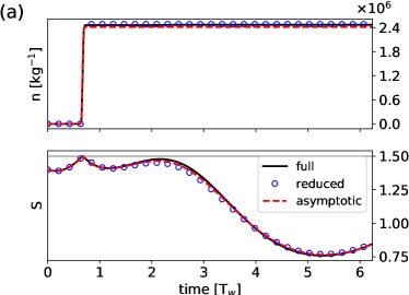
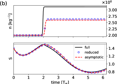
Figure 1: Time evolution of number concentration $n$ and saturation ratio $S$ for two different inital conditions: $n(0)=0$ (a) and $n(0)=2\times 10^{6}$ kg^-1 (b). $T_{w}=500$ s and initial phase of the wave $\phi=-\frac{11\pi}{20}$

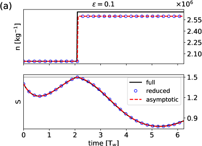
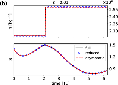
Figure 2: As in Fig. 1b but for ${\varepsilon}=10^{-1}$ (a) and ${\varepsilon}=10^{-2}$ (b); in Fig. 1b ${\varepsilon}=1$.

Since the phase of the GW is typically unknown in coarse models, we study the sensitivity of the results with respect to this parameter. For that purpose we vary the GW phase at the initial time $t=0$ and determine the nucleated ice crystals within one wave period for an initial condition $n(0)=0$. From Fig. 3 it is visible that the asymptotic solution captures for all GW phases the number of nucleated ice crystals in the full model. In addition, the values of $n$ are limited from above by the asymptotic estimate $N^{max}_{post}$.

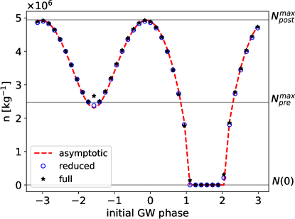
Figure 3: Nucleated number concentration, $n$, as a function of the initial GW phase. Grey horizontal lines denote the initial condition $n(0)$ and the asymptotic estimates $N^{max}_{pre}$ and $N^{max}_{post}$ from equations (91) and (92), respectively.

In Fig. 4 the normalized vertical velocity at the nucleation time is displayed. It suggests that nucleation takes place at sufficiently high updrafts but not necessary at the maximal.

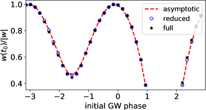
Figure 4: Normalized GW vertical velocity at $t_{0}$ as a function of the initial GW phase for the simulations from Fig. 3.

Fig. 5 summarizes the dependence of the nucleated ice crystals on the initial number concentration. The asymptotic solution reproduces nearly exactly $n$ from the reduced model. Both models are very close to the full model for $n(0)$ well below $N^{max}_{pre}$, however, for $n(0)$ approaching $N^{max}_{pre}$ they underestimate $n$ for some GW phases. The detailed evolution of the solutions for one such particular case (dashed line in Fig. 5b) was shown in Fig. 1b. As shown in Fig. 2 the discrepancy in the models results from the finite time scale separation between processes and diminishes for ${\varepsilon}\to 0$. Further, one observes in Fig. 5 that the asymptotic solution is able to capture regimes without nucleation events, too.

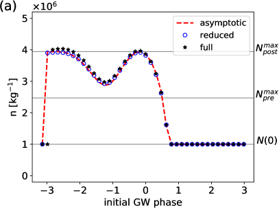
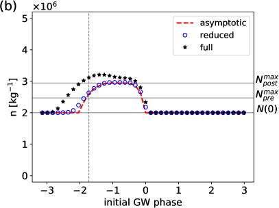
Figure 5: As in Fig. 3 but for initial number concentration $n(0)=10^{6}$ kg^-1 (a) and $n(0)=2\times 10^{6}$ kg^-1 (b). In Fig. (b) the initial $n$ is the same as the one used in Fig. 1b and 2; the dashed gray vertical line marks the initial phase used for the simulation in Fig. 1b and 2.

5 The effect of variable ice crystal mean mass in the deposition

Performing realistic air parcel simulations with a box model and a bulk microphysics scheme, BS19 demonstrated that for a wide variety of environmental conditions the constant mean mass assumption in the deposition term is a reasonable approximation during nucleation. However, right before a nucleation event where the saturation ratio is above one, the mean mass of the ice crystals will grow leading to an increased deposition term, see the $\bar{m}$ dependence in (29). The increased deposition will influence the saturation ratio, which on the other hand will affect the number of nucleated ice crystals. Since the mean mass of the ice crystals can be diagnosed from the relation $m=q/n$ for $n>0$, such effects can be incorporated in the present model if the substitution $\bar{m}=m(t)=q/n$ is introduced in the diffusional growth term. By considering again only the dominant terms in the prognostic equations, this results in the following system of reduced equations with variable mean mass in the deposition

$${\frac{dn}{dt}} =\frac{J^{*}}{{\varepsilon}}\exp\left(\frac{B^{*}}{{\varepsilon}^{2}}(S-S_{c})\right)$$ (104)

$${\frac{dS}{dt}} =\leavevmode{-D^{*}\left(\frac{q}{n}\right)^{\frac{1}{3}}(S-1)n+SF^{*}(t)}\,,$$ (105)

$${\frac{dq}{dt}} =\frac{D^{*}}{{\varepsilon}}\left(\frac{q}{n}\right)^{\frac{1}{3}}(S-1)n\,.$$ (106)

In Fig. 6 we show simulations of the reduced model with constant and with variable mean mass, in both cases the ice crystal mass is diagnosed using $m=q/n$. The vertical velocity amplitude is set to $1.25$ ms^-1 corresponding to $0.9W_{c}$. The initial conditions for all models are set to $S(0)=1.45$, $n(0)=10^{6}$ kg^-1 and $\phi=0$.

In Fig. 6 an increase of the ice crystal mass is observed before the nucleation event. Taking this into account with the model (104)-(106) results in larger number of nucleated ice particles, as compared to the constant mass model. The asymptotic solution for the constant mass case (denoted with “asym. $m_{0}$ “ in the Figure) reproduces the behavior of the constant mass reduced model and underestimates $n$, as well. In the following, we extend the asymptotic approach to allow for variable mean mass effects.

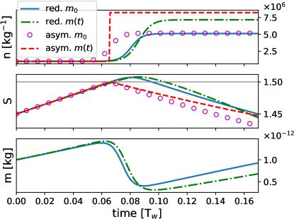
Figure 6: Time evolution of number concentration $n$, saturation ratio $S$ and mean ice mass $m$ computed for different models: the reduced model with constant mass (93)-(95), the reduced model with variable mass (104)-(106), the asymptotic solution for constant mass Sec. 33.8 and the asymptotic solution with variable mass correction (117). Note that for the latter model only the pre- and post-nucleation values are plotted, resulting in jump at $t_{0}$. The mean mass in the reduced models is diagnosed using $m=q/n$. In the figure’s legend $m_{0}$ and $m(t)$ denote models with constant and variable mass, respectively.

5.1 Pre-nucleation regime

The fully coupled system (104)-(106) involves an additional fast time scale in the $q$-equation as compared to the constant mean mass case discussed in Sec. 3. The new time scale will induce in general nontrivial dynamics on longer time scales, however, the corresponding rigorous asymptotic analysis is out of the scope of this paper. As we will show here, the asymptotic pre-nucleation solution for the constant mass case can still be used for variety of configurations if appropriate corrections are introduced.

First, we observe in Fig. 6 that before nucleation the solution for $S$ does not change much if the variable mean mass effect is taken into account. In such situations, one can use the asymptotic solution (66) for $S$ to compute the time, $t_{0}$, of the nucleation event from (88). For $S-S_{c}={O}\!\left(1\right)<0$ the right-hand-side of (104) vanishes at leading order, implying the constant solution $n(t)=N_{pre}$. Using the latter result and integrating (106) from $t_{*}$ up to $t_{0}$, we obtain at the end of the pre-nucleation regime

$$q(t_{0})^{\frac{2}{3}}=\frac{3D^{*}}{2{\varepsilon}}N_{pre}^{\frac{2}{3}}\int\limits_{t_{*}}^{t_{0}}dt^{\prime}(S(t^{\prime})-1)+q(t_{*})^{\frac{2}{3}}\,,$$ (107)

with $S(t)$ from (66).

5.2 Nucleation regime

Next, we consider the nucleation regime. On the fast nucleation time $\tau$ we have the following system of equations

$${\frac{dn}{d\tau}} ={\varepsilon}J^{*}\exp\left(\frac{B^{*}}{{\varepsilon}^{2}}(S-S_{c})\right)$$ (108)

$${\frac{dS}{d\tau}} =\leavevmode{-{\varepsilon}^{2}D^{*}\left(\frac{q}{n}\right)^{\frac{1}{3}}(S-1)n+{\varepsilon}^{2}SF^{*}(t_{0}+{\varepsilon}^{2}\tau)\,,}$$ (109)

$${\frac{dq}{d\tau}} ={\varepsilon}D^{*}\left(\frac{q}{n}\right)^{\frac{1}{3}}(S-1)n$$ (110)

From (110) we see that the leading order ice mixing ratio is constant during nucleation

$$q^{(0)}(\tau)=q^{(0)}_{pre}(t_{0})\,,$$ (111)

with the value of $q^{(0)}_{pre}(t_{0})$ from (107). Next, by repeating the manipulations in equations (143) to (147), one obtains from (108), (109) the following evolution equation for the number concentration

$${\frac{dn^{(0)}}{d\tau}}+\tilde{\delta}(n^{(0)})^{5/3}-\gamma n^{(0)}=\tilde{\mu}\,,$$ (112)

with the constant

$$\tilde{\delta} =\frac{3}{5}\left(q^{(0)}\right)^{1/3}B^{*}D^{*}(S_{c}-1)$$ (113)

and $\gamma$ defined in (77) (see below (117) for the definition of $\tilde{\mu}$). Eq (112) can be solved numerically to find the number concentration during the nucleation regime. The numerical integration of the ODE can be avoided if only the final $n$ at the end of the nucleation is of interest. Proceeding as in Sec. 33.6 we have the following matching conditions for the pre-nucleation, nucleation and post-nucleation regime

$$n^{(0)}_{nuc}(-\infty) =N_{pre}\,,$$ (114)

$$n^{(0)}_{nuc}(\infty) =N_{post}\,,$$ (115)

$${\frac{dn^{(0)}_{nuc}}{d\tau}}(\pm\infty) ={\frac{dn^{(0)}_{pre}}{dt}}(t_{0})={\frac{dn^{(0)}_{post}}{dt}}(t_{0})=0$$ (116)

Inserting the matching conditions in (112) leads to an algebraic equation for $N_{post}$

$$\tilde{\delta}N_{post}^{5/3}-\gamma N_{post}=\tilde{\mu}\,,$$ (117)

where $\tilde{\mu}=\tilde{\delta}N_{pre}^{5/3}-\gamma N_{pre}$. Note that for $N_{pre}=0$, (117) implies for the dependence of $N_{post}$ on the GW vertical velocity: $N_{post}\sim\hat{w}^{3/2}$, which is consistent with the scaling in Kärcher and Lohmann (2002).

5.3 Numerical results

Equation (117) is used to find an asymptotic approximation of the nucleated number concentration, the comparison with the numerical results is shown in Fig. 6. The current procedure allows to produce larger number of nucleated ice crystals as compared with the constant mass model, the magnitude of $n$ is close to the one of the variable mean mass model.

The performance of the current approach is systematically evaluated by varying the initial GW phase. The corresponding results are summarized in Fig. 7. The figure suggests that the proposed procedure captures the number of ice crystals after nucleation for various initial GW phases.

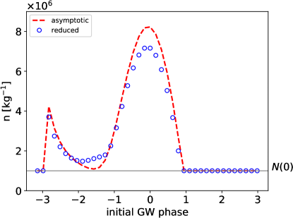
Figure 7: Number concentration $n$ as a function of the initial GW phase for the variable mean mass model (104)-(106) and for the asymptotic solution (117) from Sec. 5. Initial conditions as in Fig. 6.

A note of caution should be added on the relevance of the variable mean mass model presented in this section. The use of the pre-nucleation $S$ from (66) in (107) might be not valid on longer time scales, see the first paragraph of Sec. 5a. Further, Fig. 6 suggests that there might be situations with considerable growth of $m$ before nucleation takes place. Obviously, for large $m$ the sedimentation term will provide a sink for the mean mass: see (42). The correct incorporation of the sedimentation effects will be subject of a future study.

6 Ice physics forced by superposition of gravity waves

In this section we consider the case when a GW spectrum is forcing the ice physics. The GW forcing is constructed by considering $N_{GW}$ waves with vertical wind amplitudes sampled from a white frequency spectrum in accordance with observations (Podglajen et al. 2016). The wave amplitudes $\hat{w}$ are rescaled such that the total GW momentum flux, $\rho u^{\prime}w^{\prime}$, equals 5 mPa at 8 km altitude. This value for the momentum flux is within the range given by observational and modeling studies (Hertzog et al. 2012; Kim et al. 2021; Corcos et al. 2021). For high-frequency GW (with $T_{w}\sim N$) in the tropopause region the ratio

$$\frac{T_{d}}{T_{w}}={O}\!\left({\varepsilon}^{-1}\right)$$ (118)

is more appropriate, compare the last equation with (56). In this case, one obtains from (57)

$${\frac{D\pi}{Dt_{d}}}=\left({\varepsilon}^{1+\alpha}{\frac{D\pi^{\prime}}{Dt_{w}}}+{\varepsilon}w{\frac{d\bar{\pi}}{dz_{s}}}\right)\,,$$ (119)

implying that the tendency of $\pi^{\prime}$ is of the same order as the vertical advection term for $\alpha=0$. It was verified that the magnitude of the wave amplitudes allows to neglect the nonlinear advection term and the term ${\frac{\partial\pi^{\prime}}{\partial t}}$ will have the dominant contribution in the material derivative of $\pi^{\prime}$. In order to account for effects due the high-frequency waves, we will include the latter term into the GW forcing term. We will also include a next order correction term by keeping the $c_{p}/R$ term in equation (43), since we found that this improves the results for the general case of superposition of GW. We found from simulations that the magnitudes of the waves are too small to trigger nucleation, because of this we include a constant vertical updraft $w_{00}$=2 cm s^-1 on which the GW are superimposed. With the assumptions above, the forcing (64) is generalized to

$$F^{*}(t_{w})=\left(L^{*}-{\varepsilon}\frac{c_{p}}{R}\right)\left\{\sum\limits_{j}^{N_{GW}}\left[\frac{R}{c_{p}}|\tilde{w}_{j}^{(0)}|\cos(\omega_{j}t_{w}+\phi_{j})+\omega_{j}|\tilde{\pi}_{j}^{(0)}|\sin(\omega_{j}t_{w}+\phi_{j})\right]+\frac{R}{c_{p}}w_{00}\right\}$$ (120)

With the new forcing (120) we compute the ice crystal number concentration using the asymptotic solution from Section 33.8. We perform $10^{3}$ realizations, each forced by a superposition of $10$ waves with random frequencies uniformly distributed within the range $\omega_{min}<\omega_{j}<\omega_{max}$. A random wave phase increment $\delta\phi_{j}=\phi_{j}-\mathbf{x}(t_{*})\cdot\mathbf{k}_{j}$ is uniformly distributed within $[0,2\pi]$. The vertical wavelength of all waves is set to 1 km and the initial values $n=q=0$ and $S=1.4$ are used in the simulations.

The results are summarized in Fig. 8a for the case where $\omega_{j}$ is drawn from a narrow range around the frequency $T_{w}^{-1}=2\times 10^{-3}$ s^-1 for which the asymptotic analysis was performed. The asymptotic solution captures the ice crystal number concentration, $n$, from the full model for the majority of realizations. The accuracy increases if large values of $n$ are nucleated. Further, by reordering $n$ from the asymptotic solution in ascending order (the dashed black line in Fig. 8a), we see that the distribution produced by the asymptotic model is identical with the one from the full model (cyan line). This is an important result for the application of the present asymptotic solutions in climate models. Since the phase of the waves is typically unknown, any parameterization will not be able to reproduce the exact nucleation time $t_{0}$. However, on average our model produces a distribution of $n$ matching the one from the full model.

Next, we consider the full frequency range of GW, the corresponding results are summarized in Fig. 8b. It has to be stressed, that our asymptotic analysis is only valid for the frequency range around $T_{w}^{-1}$. However, the asymptotic model can still capture many of the nucleation events of the full model. Again, this is particularly valid for the largest value $10^{6}<n<10^{7}$, which will probably be the more relevant. For smaller values of $n$ the quality of prediction deteriorates. Reordering of the asymptotic values reveals a small positive bias in the distribution produced by the asymptotic model. We suppose that this bias might be due to small amplitudes of the GW, inconsistent with our scaling where $\hat{w}\sim W_{c}$ was assumed, and the omission of the low-frequency GW in the asymptotic analysis.

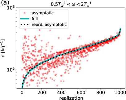
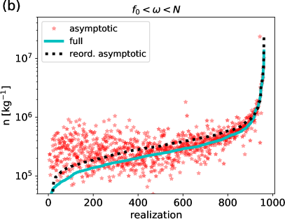
Figure 8: Nucleated number concentration, $n$, for $10^{3}$ different realizations of a superposition of GW with frequencies: $0.5T^{-1}_{w}<\omega<2T^{-1}_{w}$ (a) and $f_{0}<\omega<N$ (b). The cyan line shows in ascending order the results from the full model. The corresponding asymptotic solutions are shown as red stars. The dashed black line displays the same asymptotic solutions but after sorting them in ascending order.

7 Conclusions

We present an asymptotic approach allowing to identify a reduced model for the self-consistent description of ice physics forced by a superposition of GW including the effect of diffusional growth and homogeneous nucleation of ice crystals. Further, using matched asymptotic techniques analytical solutions are constructed, involving a novel parameterization (90) for the ice crystal number concentration $n$. The latter has as input parameters the wave amplitudes and phases, and the time of the nucleation event. It allows the derivation of upper bound for the nucleated $n$, as well as, a threshold for the initial $n$ which will inhibit nucleation. The numerical simulations with a Lagrangian parcel model show that the parameterization reproduces nucleation events triggered by a monochromatic GW for a variety of initial conditions. Further, in the case of superposition of GW within the mid-frequency range the parameterization generates a distribution of $n$ matching the one of the full model. By extending the parameterization to high-frequency GW it is shown that the asymptotic solution produces distribution similar to the one of the full model even if the complete GW frequency spectrum is used as forcing. The results presented here demonstrate the potential of our approach for constructing improved cirrus schemes in climate models with realistic GW variability as simulated with transient GW parameterizations (Bölöni et al. 2021; Kim et al. 2021).

When comparing the treatment of the ice physics in our approach with the one from BS19, we observe different scaling in the nucleation term: in the latter work $J\sim B\sim{\varepsilon}^{-1}$ is used, whereas here we apply $J\sim{\varepsilon}^{-1},B\sim{\varepsilon}^{-2}$. Nevertheless, our parameterization (90) is equivalent to the closure of BS19 for constant updraft velocity if the velocity there is replaced by the GW vertical velocity at the nucleation time $t_{0}$. This is not surprising, since the GW nearly does not vary on the fast nucleation time scale. The correspondence of the two parameterizations becomes more clear if one takes into account that in BS19 ${\varepsilon}={O}\!\left(10^{-2}\right)$ and here ${\varepsilon}={O}\!\left(10^{-1}\right)$, implying the same magnitude of the nucleation exponent $B$ under the different scalings. As shown by Spichtinger et al. (2023) the exact value of the nucleation rate $J$ is not crucial as long as it is sufficiently large. Still, we have to stress that the present approach generalizes the framework of BS19 to include wave dynamics and the consistency between the two parameterizations only supports our results. In addition, we derive a novel parameterization for the variable mean mass model, see (117), a threshold for nucleation inhibition, $N^{max}_{pre}$ from (92), and an high-frequency correction to the parameterization, (120).

The present asymptotic solutions are applicable mainly to the mid-frequency GW in the troposphere and tropopause region, as well as, to high-frequency GW in the troposphere. For high-frequency GW in the tropopause region the ratio between the time scale of the diffusional growth and of the wave is given by $T_{d}/T_{w}\sim{\varepsilon}^{-1}$. The simulations from Sec. 6 shows large numbers of $n$ if the high-frequency GW are included. This suggests a new regime dominated by the GW forcing term and we propose some asymptotic corrections to account for it. We expect that this regime corresponds to the temperature-limit events studied in Dinh et al. (2016). For low-frequency GW the scaling $T_{d}/T_{w}\sim{\varepsilon}$ is appropriate. In this case the GW forcing term becomes by a factor of ${\varepsilon}$ weaker, when compared to the depositional growth term. This regime is relevant for low updraft velocities and will be considered in an upcoming study.

Our asymptotic analysis assumes a reference number concentration, $n_{c}$. However, the results from Sec. 6 suggest that the resulting asymptotic model is valid for a wider range of $n$. If regimes with other values of $n_{c}$ are of interest, the present asymptotic framework can be adapted for the systematic investigation of these too.

The models presented here predict for the particular GW forcings values of $n$ which are within or at the upper range of observations, e.g., see Fig. 8 from Krämer et al. (2020). However, a direct comparison with observational data is hampered for two main reasons. First, most of the measurements lack information on the wave properties, e.g., wave amplitude and frequency, so the GW forcing cannot be determined. Second, nucleation takes place at very fast time scale and within a confined spatial region. Therefore, the vast majority of measurements of ice crystals are taken probably after the nucleation event happened. However, at later stages of the ice cloud life cycle, other processes such as sedimentation are determining the microphysical properties. The latter lead to smearing of the clear nucleation signature and to significantly smaller $n$ values (see, e.g., Spichtinger and Gierens 2009); this effect is enhanced if ice crystals fall into subsaturated air and thus evaporate. This might explain, why high number densities are quite rarely observed (see, e.g., Krämer et al. 2009, 2020).

In the present regime the magnitude of the sedimentation effects is determined by the sedimentation time scale $T_{sed}=H_{c}/c_{q}m_{c}^{2/3}$. Substituting the reference quantities gives $T_{sed}\sim{\varepsilon}^{-2}T_{d}\sim 11$ h, implying that at leading order sedimentation is negligible compared to the diffusional growth term. Note however, that $T_{sed}$ will decrease if regimes with larger ice crystal mass, $m_{c}$, or smaller vertical scales, $H_{c}$, are of interest. As shown in Podglajen et al. (2018), sedimentation modulated by GW forcing produces localization effects in cirrus.

In the present study only cirrus formed by homogeneous nucleation are considered, since this is the dominant formation mechanism in the cold temperature regime with strong updraft velocities (e.g., Heymsfield and Miloshevich 1993). Still, heterogeneous nucleation can considerably alter cirrus formation (see, e.g., Gierens 2003; Spichtinger and Cziczo 2010); however, the important feature is, also in case of competing nucleation pathways, the occurrence of pre-existing ice crystals, as in our investigations. In addition, turbulence due to GW breaking is another source of GW generated variability omitted in the present study (e.g., Atlas and Bretherton 2023).

$$S=\frac{q_{v}p}{p_{si}}\,.$$ (121)

Applying ${\frac{d}{dt_{d}}}$ to (121) yields

$${\frac{DS}{Dt_{d}}} =\frac{p}{p_{si}}{\frac{Dq_{v}}{Dt_{d}}}+\frac{S}{p}{\frac{Dp}{Dt_{d}}}-\frac{S}{p_{si}}{\frac{Dp_{si}}{Dt_{d}}}$$ (122)

$$=\frac{p}{p_{si}}{\frac{Dq_{v}}{Dt_{d}}}+\frac{c_{p}S}{R\pi}{\frac{D\pi}{Dt_{d}}}-\frac{SL^{*}}{{\varepsilon}T^{2}}{\frac{DT}{Dt_{d}}}$$ (123)

$$=\frac{p}{p_{si}}{\frac{Dq_{v}}{Dt_{d}}}+\frac{c_{p}S}{R\pi}{\frac{D\pi}{Dt_{d}}}-\frac{SL^{*}}{{\varepsilon}T^{2}}\left(\pi\underbrace{{\frac{D\theta}{Dt_{d}}}}_{=0}+\theta{\frac{D\pi}{Dt_{d}}}\right)$$ (124)

$$=\frac{p}{p_{si}}{\frac{Dq_{v}}{Dt_{d}}}-\frac{S}{\pi}{\frac{D\pi}{Dt_{d}}}\left(\frac{L^{*}}{{\varepsilon}T}-\frac{c_{p}}{R}\right)$$ (125)

where (40) was used to obtain (123), (22) in (124) and the definition of potential temperature $\theta=T/\pi$ for the last equation (125). With this one obtains (43).

[B] GW dispersion relation and polarization relations

With $\mathbf{v}=\mathbf{v}^{(0)}+{O}\!\left({\varepsilon}\right)$ the leading order continuity equation reads

$$\nabla\cdot\mathbf{v}^{(0)}=0.$$ (126)

Using the wave ansatz for $\mathbf{v}^{(0)}$, this gives the solenoidality condition

$$\mathbf{k}\cdot\tilde{\mathbf{v}}^{(0)}=0\,,$$ (127)

implying that the wavevector $\mathbf{k}$ and $\tilde{\mathbf{v}}^{(0)}$ are orthogonal. The latter property will be used to eliminate nonlinear advection terms in the equations.

From the leading order vertical momentum equation we obtain hydrostatic balance between $\bar{\pi}^{(0)}$ and $\bar{\theta}^{(0)}$

$${\frac{d\bar{\pi}^{(0)}}{dz_{s}}}=-\frac{R}{c_{p}\bar{\theta}^{(0)}}\,.$$ (128)

Similarly, the next order vertical momentum balance reads

$${\frac{d\bar{\pi}^{(1)}}{dz_{s}}}=\frac{R\bar{\theta}^{(1)}}{c_{p}\bar{\theta}^{(0)^{2}}}\,,$$ (129)

where we have used (128). Note, that in the case $\alpha=\beta=0$ there is no advection term appearing in the latter equation due to (127).

The projection of the leading order equations onto the GW field reads

$${\frac{\partial\mathbf{u}^{(0)}}{\partial t_{w}}} =-\frac{c_{p}\bar{\theta}^{(0)}}{R}\nabla_{h}\pi^{(2+\alpha)}$$ (130)

$$(1-\beta){\frac{\partial w^{(0)}}{\partial t_{w}}} =-\frac{c_{p}\bar{\theta}^{(0)}}{R}{\frac{\partial\pi^{(2+\alpha)}}{\partial z_{w}}}+\frac{\theta^{(1+\alpha)}}{\bar{\theta}^{(0)}}$$ (131)

$$\nabla_{w}\cdot\mathbf{v}^{(0)} =0\,,$$ (132)

$${\frac{\partial\theta^{(1+\alpha)}}{\partial t_{w}}}+w^{(0)}{\frac{d\bar{\theta}^{(\alpha)}}{dz_{s}}} =0\,,$$ (133)

where again (127) was utilized. Inserting in eqs. (130)-(133) a wave ansatz for the solution, one obtains the following system of linear equations for the wave amplitudes

$$\bm{\mathsf{M}}\mathbf{z}=0$$ (134)

where

$$\bm{\mathsf{M}}=\left(\begin{array}[h]{c c c c c}-i\omega&0&0&0&ik\\ 0&-i\omega&0&0&il\\ 0&0&-i(1-\beta)\omega&-\bar{N}&im\\ 0&0&\bar{N}&-i\omega&0\\ ik&il&im&0&0\end{array}\right)$$ (140)

with $\mathbf{z}=(\tilde{u}^{(0)},\tilde{v}^{(0)},\tilde{w}^{(0)},\tilde{b}^{(1+\alpha)}/\bar{N},\frac{c_{p}}{R}\bar{\theta}^{(0)}\tilde{\pi}^{(2+\alpha)})$ and

$$\bar{N}^{2} =\frac{1}{\bar{\theta}^{(0)}}{\frac{d\bar{\theta}^{(\alpha)}}{dz}}$$ (141)

$$\tilde{b}^{(1+\alpha)} =\frac{\tilde{\theta}^{(1+\alpha)}}{\bar{\theta}^{(0)}}\,.$$ (142)

Looking for non-trivial solutions of (134), one derives the dispersion relation (59) and the polarization relations (58) for the GW amplitudes.

[C] Evolution equation for $n$ in the nucleation regime Here, the equation for $n$ is derived: first (72) is differentiated with respect to $\tau$ and after this the exponential function is replaced using (72) giving

$${\frac{d^{2}n}{d\tau^{2}}} =\frac{B^{*}}{{\varepsilon}^{2}}{\frac{dS}{d\tau}}{\frac{dn}{d\tau}}+{O}\!\left({\varepsilon}^{2}\right)\,.$$ (143)

Inserting (73) yields

$${\frac{d^{2}n}{d\tau^{2}}} =B^{*}{\frac{dn}{d\tau}}\left[-D^{*}(S-1)Tn-\frac{L^{*}Sw}{\bar{\pi}}{\frac{d\bar{\pi}}{dz_{s}}}\right]+{O}\!\left({\varepsilon}\right)\,.$$ (144)

The evaluation of the leading order equation takes the form

$${\frac{d^{2}n^{(0)}}{d\tau^{2}}} =B^{*}{\frac{dn^{(0)}}{d\tau}}\left[-D^{*}(S^{(0)}-1)\bar{T}^{(0)}n^{(0)}-\frac{L^{*}S^{(0)}w^{(0)}}{\bar{\pi}^{(0)}}{\frac{d\bar{\pi}^{(0)}}{dz_{s}}}\right]\,.$$ (145)

After substituting (55), (60), (128) and (64) in the last equation one yields

$${\frac{d^{2}n^{(0)}}{d\tau^{2}}} =B^{*}{\frac{dn^{(0)}}{d\tau}}\left[-D^{*}(S^{(0)}-1)n^{(0)}+\leavevmode{F^{*}(t_{0})S^{(0)}}\right]\,,$$ (146)

where the expansion: $F^{*}(t_{w})=F^{*}(t_{0})+{O}\!\left({\varepsilon}^{2}\right)$ was used. Taking into account that $S^{(0)}=S_{c}$, equation (146) can be written as

$${\frac{d}{d\tau}}\left({\frac{dn^{(0)}}{d\tau}}+\delta(n^{(0)})^{2}-\gamma n^{(0)}\right)=0$$ (147)

with the definitions introduced in (76), (77). Integrating (147) over time finally gives (75).

[D] Composite solution Despite the fact that $N_{post}$ is determined from (90), the integration constant $n_{0}$ entering (78) through (82) is still unknown. It will, however, not effect the value of $N_{post}$. Moreover, since in the present asymptotic analysis $t_{0}$ can be found up to some higher order corrections, $n_{0}$ is undetermined. To see this we introduce another constant $\tau_{0}$ defined as $C=e^{-\sigma\tau_{0}}$, we can write (78) as

$$n^{(0)}(\tau)=\frac{n_{s}+n_{e}e^{\frac{\sigma}{{\varepsilon}^{2}}(t-t_{0}-{\varepsilon}^{2}\tau_{0})}}{1+e^{\frac{\sigma}{{\varepsilon}^{2}}(t-t_{0}-{\varepsilon}^{2}\tau_{0})}}$$ (148)

Note, that from (88) $t_{0}$ is determined up to ${O}\!\left({\varepsilon}\right)$ corrections, which will result in modifications of the constant $n_{0}$. One way of setting the value for $n_{0}$ is by requiring that at $\tau=0$ the saturation ratio $S$ should reach a maximum. At the end of the pre-nucleation we have $\dot{S}>0$, on the other hand at the beginning of the post-nucleation $\dot{S}<0$, thus $S$ should have a maximum within the nucleation regime. We define $n_{0}$ by requiring that in (73) $\dot{S}=0$ at time $\tau=0$ up to ${O}\!\left({\varepsilon}^{3}\right)$ corrections. After using (55), (60), (128) (64) and (74) this implies

$$n_{0}=\frac{F^{*}(t_{0})S_{c}}{D^{*}(S_{c}-1)}\implies C=1\,.$$ (149)

The requirement of having a maximum in the saturation ratio upon the nucleation is physically meaningful and may be interpreted as the defining feature of a nucleation event.

It remains to construct the composite solution valid in all three regimes. For the number concentration the nucleation regime represents an interior layer (e.g. Holmes 2013), enclosed by the outer layers of the pre-nucleation and post-nucleation regime. In this case the composite solution reads

$$n(t_{w})=n^{(0)}_{pre}(t_{w})+n^{(0)}_{nuc}(\tau)+n^{(0)}_{post}(t_{w})-n^{(0)}_{nuc}(-\infty)-n^{(0)}_{nuc}(\infty)+{O}\!\left({\varepsilon}\right)\,.$$ (150)

Substituting (65), (78), (83) and (84) in (150) gives for the number concentration

$$n(t_{w}) =\frac{n_{s}+n_{e}e^{\frac{\sigma}{{\varepsilon}^{2}}(t_{w}-t_{0})}}{1+e^{\frac{\sigma}{{\varepsilon}^{2}}(t_{w}-t_{0})}}+{O}\!\left({\varepsilon}\right)\,.$$ (151)

Since the time derivative of the saturation ratio has a jump from the pre-nucleation to the post-nucleation value, the nucleation regime represents a corner layer for $S$ (Holmes 2013). For such a layer two cases depending on the sign of $t-t_{0}$ has to be considered when constructing the composite solution

$$S(t_{w})=\begin{cases}S^{(0)}_{pre}(t_{w})+S^{(0)}_{nuc}(\tau)-S^{(0)}_{nuc}(-\infty)\qquad&\text{ for }t_{w}\leq t_{0}\\ S^{(0)}_{post}(t_{w})+S^{(0)}_{nuc}(\tau)-S^{(0)}_{nuc}(\infty)\qquad&\text{ for }t_{w}>t_{0}\end{cases}+{O}\!\left({\varepsilon}\right)\,.$$ (152)

Substituting (66), (74) in (152), the solution for $S$ takes the form

$$S(t_{w})=\begin{cases}S_{*}S_{h}(t_{w},t_{*})+\int\limits_{t_{*}}^{t_{w}}dt^{\prime}D^{*}n_{s}S_{h}(t_{w},t^{\prime})\qquad&\text{ for }t_{w}\leq t_{0}\\ S_{c}S_{h}(t_{w},t_{0})+\int\limits_{t_{0}}^{t_{w}}dt^{\prime}D^{*}n_{e}S_{h}(t_{w},t^{\prime})\qquad&\text{ for }t_{w}>t_{0}\end{cases}+{O}\!\left({\varepsilon}\right)\,,$$ (153)

with $S_{h}$ defined in (67). [E] Description Lagrangian parcel model The Lagrangian parcel model describes the evolution of $n,q$ and $q_{v}$ in an air parcel oscillating in the $x-z$ plane under the gravity wave forcing. It solves (37)-(39) with sedimentation switched off, i.e., $S^{*}_{n}=S^{*}_{q}=0$. The parcel position vector, $\mathbf{x}(t)=(x,z)^{T}$, is determined from

$$\frac{d\mathbf{x}}{dt}=\mathbf{v},$$ (154)

where the velocity field is given in general by a superposition of GWs with a possibility to include a constant updraft velocity, $w_{00}$,

$$\mathbf{v}=\sum_{j}^{N_{GW}}\mathbf{\tilde{v}}_{j}\cos\left(\omega_{j}t+k_{j}x+m_{j}z+\delta\phi_{j}\right)+w_{00}\mathbf{e}_{z}\,.$$ (155)

Each frequency $\omega_{j}$ and amplitude $\mathbf{\tilde{v}}_{j}$ is satisfying the general inertial GW dispersion relation and polarization relation (e.g. Achatz 2022) with $N=0.02$ s^-1 for the the tropopause region. A vertical wavelength of 1 km is assumed, comparable to the value of 3 km used in the study of Corcos et al. (2023).

From (154) with initial condition $z=z_{00}$ and $x=x_{00}$ the parcel position is found. With this the wave fluctuations of Exner pressure, $\pi^{\prime}$, and of potential temperature, $\theta^{\prime}$, are determined from the corresponding polarization relations. To those fluctuations one has to add the stationary contributions $\bar{\pi}$ and $\bar{\theta}$ from the reference atmosphere in order to determine the full fields. It is assumed that in the vicinity of $z_{00}$ the reference atmosphere can be represented by an isothermal temperature profile $\bar{T}(z)=T_{00}$ with corresponding pressure $\bar{p}(z)=p_{00}e^{-\frac{z-z_{00}}{H_{p}}}$ (all in dimensional form). From those the Exner pressure, $\bar{\pi}$, and pontential temperature, $\bar{\theta}$, of the reference atmosphere are calculated using the definitions $T=\pi\theta$ and $\pi=(p/p_{00})^{R/c_{p}}$. By adding all together one obtains the total fields $\pi$ and $\theta$, or equivalently $p$ and $T$. Finally, the saturation pressure can be determined from (54). In practice, equations (37)-(39) and (58) are simultaneously integrated numerically and we use the above mentioned procedure to find $p$, $p_{si}$ and $T$ at each time step.

References

- Achatz (2022) Achatz, U., 2022: Atmospheric Dynamics. Springer Berlin Heidelberg, Berlin, Heidelberg, 10.1007/978-3-662-63941-2, URL https://link.springer.com/10.1007/978-3-662-63941-2.
- Achatz et al. (2010) Achatz, U., R. Klein, and F. Senf, 2010: Gravity waves, scale asymptotics and the pseudo-incompressible equations. Journal of Fluid Mechanics, 663, 120–147, 10.1017/S0022112010003411, URL https://www.cambridge.org/core/product/identifier/S0022112010003411/type/journal˙article.
- Achatz et al. (2017) Achatz, U., B. Ribstein, F. Senf, and R. Klein, 2017: The interaction between synoptic‐scale balanced flow and a finite‐amplitude mesoscale wave field throughout all atmospheric layers: weak and moderately strong stratification. Quarterly Journal of the Royal Meteorological Society, 143 (702), 342–361, 10.1002/qj.2926, URL https://onlinelibrary.wiley.com/doi/10.1002/qj.2926.
- Atlas and Bretherton (2023) Atlas, R., and C. S. Bretherton, 2023: Aircraft observations of gravity wave activity and turbulence in the tropical tropopause layer: prevalence, influence on cirrus clouds, and comparison with global storm-resolving models. Atmospheric Chemistry and Physics, 23 (7), 4009–4030, 10.5194/acp-23-4009-2023, URL https://acp.copernicus.org/articles/23/4009/2023/.
- Baumgartner et al. (2022) Baumgartner, M., C. Rolf, J.-U. Grooß, J. Schneider, T. Schorr, O. Möhler, P. Spichtinger, and M. Krämer, 2022: New investigations on homogeneous ice nucleation: the effects of water activity and water saturation formulations. Atmospheric Chemistry and Physics, 22 (1), 65–91, 10.5194/acp-22-65-2022, URL https://acp.copernicus.org/articles/22/65/2022/, publisher: Copernicus GmbH.
- Baumgartner and Spichtinger (2019) Baumgartner, M., and P. Spichtinger, 2019: Homogeneous nucleation from an asymptotic point of view. Theoretical and Computational Fluid Dynamics, 33 (1), 83–106, 10.1007/s00162-019-00484-0, URL http://link.springer.com/10.1007/s00162-019-00484-0.
- Baumgartner et al. (2020) Baumgartner, M., R. Weigel, A. H. Harvey, F. Plöger, U. Achatz, and P. Spichtinger, 2020: Reappraising the appropriate calculation of a common meteorological quantity: potential temperature. Atmospheric Chemistry and Physics, 20 (24), 15 585–15 616, 10.5194/acp-20-15585-2020, URL https://acp.copernicus.org/articles/20/15585/2020/, publisher: Copernicus GmbH.
- Bramberger et al. (2022) Bramberger, M., and Coauthors, 2022: First Super-Pressure Balloon-Borne Fine-Vertical-Scale Profiles in the Upper TTL: Impacts of Atmospheric Waves on Cirrus Clouds and the QBO. Geophysical Research Letters, 49 (5), e2021GL097 596, 10.1029/2021GL097596, URL https://onlinelibrary.wiley.com/doi/abs/10.1029/2021GL097596, _eprint: https://onlinelibrary.wiley.com/doi/pdf/10.1029/2021GL097596.
- Bölöni et al. (2021) Bölöni, G., Y.-H. Kim, S. Borchert, and U. Achatz, 2021: Toward Transient Subgrid-Scale Gravity Wave Representation in Atmospheric Models. Part I: Propagation Model Including Nondissipative Wave–Mean-Flow Interactions. Journal of the Atmospheric Sciences, 78 (4), 1317–1338, 10.1175/JAS-D-20-0065.1, URL https://journals.ametsoc.org/view/journals/atsc/78/4/JAS-D-20-0065.1.xml, publisher: American Meteorological Society Section: Journal of the Atmospheric Sciences.
- Bölöni et al. (2016) Bölöni, G., B. Ribstein, J. Muraschko, C. Sgoff, J. Wei, and U. Achatz, 2016: The Interaction between Atmospheric Gravity Waves and Large-Scale Flows: An Efficient Description beyond the Nonacceleration Paradigm. Journal of the Atmospheric Sciences, 73 (12), 4833–4852, 10.1175/JAS-D-16-0069.1, URL https://journals.ametsoc.org/view/journals/atsc/73/12/jas-d-16-0069.1.xml, publisher: American Meteorological Society Section: Journal of the Atmospheric Sciences.
- Corcos et al. (2021) Corcos, M., A. Hertzog, R. Plougonven, and A. Podglajen, 2021: Observation of Gravity Waves at the Tropical Tropopause Using Superpressure Balloons. Journal of Geophysical Research: Atmospheres, 126 (15), e2021JD035 165, 10.1029/2021JD035165, URL https://onlinelibrary.wiley.com/doi/abs/10.1029/2021JD035165, _eprint: https://onlinelibrary.wiley.com/doi/pdf/10.1029/2021JD035165.
- Corcos et al. (2023) Corcos, M., A. Hertzog, R. Plougonven, and A. Podglajen, 2023: A simple model to assess the impact of gravity waves on ice crystal populations in the tropical tropopause layer. preprint, Clouds and Precipitation/Atmospheric Modelling and Data Analysis/Stratosphere/Physics (physical properties and processes). 10.5194/egusphere-2022-1444, URL https://egusphere.copernicus.org/preprints/2023/egusphere-2022-1444/.
- Dean et al. (2007) Dean, S. M., J. Flowerdew, B. N. Lawrence, and S. D. Eckermann, 2007: Parameterisation of orographic cloud dynamics in a GCM. Climate Dynamics, 28 (6), 581–597, 10.1007/s00382-006-0202-0, URL http://link.springer.com/10.1007/s00382-006-0202-0.
- Dinh et al. (2016) Dinh, T., A. Podglajen, A. Hertzog, B. Legras, and R. Plougonven, 2016: Effect of gravity wave temperature fluctuations on homogeneous ice nucleation in the tropical tropopause layer. Atmospheric Chemistry and Physics, 16 (1), 35–46, 10.5194/acp-16-35-2016, URL https://acp.copernicus.org/articles/16/35/2016/, publisher: Copernicus GmbH.
- Durran (1989) Durran, D. R., 1989: Improving the Anelastic Approximation. Journal of the Atmospheric Sciences, 46 (11), 1453–1461, 10.1175/1520-0469(1989)046¡1453:ITAA¿2.0.CO;2, URL https://journals.ametsoc.org/view/journals/atsc/46/11/1520-0469˙1989˙046˙1453˙itaa˙2˙0˙co˙2.xml, publisher: American Meteorological Society Section: Journal of the Atmospheric Sciences.
- Gasparini et al. (2018) Gasparini, B., A. Meyer, D. Neubauer, S. Münch, and U. Lohmann, 2018: Cirrus Cloud Properties as Seen by the CALIPSO Satellite and ECHAM-HAM Global Climate Model. Journal of Climate, 31 (5), 1983–2003, 10.1175/JCLI-D-16-0608.1, URL https://journals.ametsoc.org/doi/10.1175/JCLI-D-16-0608.1.
- Gierens (2003) Gierens, K., 2003: On the transition between heterogeneous and homogeneous freezing. Atmospheric Chemistry and Physics, 3 (2), 437–446, 10.5194/acp-3-437-2003, URL https://acp.copernicus.org/articles/3/437/2003/.
- Haag and Kärcher (2004) Haag, W., and B. Kärcher, 2004: The impact of aerosols and gravity waves on cirrus clouds at midlatitudes. Journal of Geophysical Research, 109, D12 202, 10.1029/2004JD00457.
- Hertzog et al. (2012) Hertzog, A., M. J. Alexander, and R. Plougonven, 2012: On the Intermittency of Gravity Wave Momentum Flux in the Stratosphere. Journal of the Atmospheric Sciences, 69 (11), 3433–3448, 10.1175/JAS-D-12-09.1, URL https://journals.ametsoc.org/doi/10.1175/JAS-D-12-09.1.
- Heymsfield and Miloshevich (1993) Heymsfield, A. J., and L. M. Miloshevich, 1993: Homogeneous Ice Nucleation and Supercooled Liquid Water in Orographic Wave Clouds. Journal of the Atmospheric Sciences, 50 (15), 2335–2353, 10.1175/1520-0469(1993)050¡2335:HINASL¿2.0.CO;2, URL https://journals.ametsoc.org/view/journals/atsc/50/15/1520-0469˙1993˙050˙2335˙hinasl˙2˙0˙co˙2.xml, publisher: American Meteorological Society Section: Journal of the Atmospheric Sciences.
- Holmes (2013) Holmes, M. H., 2013: Introduction to Perturbation Methods. Texts in Applied Mathematics, 20, Springer.
- Hoose and Möhler (2012) Hoose, C., and O. Möhler, 2012: Heterogeneous ice nucleation on atmospheric aerosols: a review of results from laboratory experiments. Atmospheric Chemistry and Physics, 12, 9817–9854.
- Jensen and Pfister (2004) Jensen, E., and L. Pfister, 2004: Transport and freeze-drying in the tropical tropopause layer. Journal of Geophysical Research, 109 (D02207), 10.1029/2003JD004022.
- Joos et al. (2009) Joos, H., P. Spichtinger, and U. Lohmann, 2009: Orographic cirrus in a future climate. Atmospheric Chemistry and Physics, 9 (20), 7825–7845, 10.5194/acp-9-7825-2009, URL https://acp.copernicus.org/articles/9/7825/2009/.
- Joos et al. (2008) Joos, H., P. Spichtinger, U. Lohmann, J.-F. Gayet, and A. Minikin, 2008: Orographic cirrus in the global climate model ECHAM5. Journal of Geophysical Research, 113 (D18), D18 205, 10.1029/2007JD009605, URL http://doi.wiley.com/10.1029/2007JD009605.
- Kienast-Sjögren et al. (2013) Kienast-Sjögren, E., P. Spichtinger, and K. Gierens, 2013: Formulation and test of an ice aggregation scheme for two-moment bulk microphysics schemes. Atmospheric Chemistry and Physics, 13 (17), 9021–9037, 10.5194/acp-13-9021-2013, URL https://acp.copernicus.org/articles/13/9021/2013/.
- Kim et al. (2016) Kim, J.-E., and Coauthors, 2016: Ubiquitous Influence of Waves on Tropical High Cirrus Cloud. 21.
- Kim et al. (2021) Kim, Y.-H., G. Bölöni, S. Borchert, H.-Y. Chun, and U. Achatz, 2021: Toward Transient Subgrid-Scale Gravity Wave Representation in Atmospheric Models. Part II: Wave Intermittency Simulated with Convective Sources. Journal of the Atmospheric Sciences, 78 (4), 1339–1357, 10.1175/JAS-D-20-0066.1, URL https://journals.ametsoc.org/view/journals/atsc/78/4/JAS-D-20-0066.1.xml, publisher: American Meteorological Society Section: Journal of the Atmospheric Sciences.
- Koop et al. (2000) Koop, T., B. Luo, A. Tsias, and T. Peter, 2000: Water activity as the determinant for homogeneous ice nucleation in aqueous solutions. Nature, 406 (6796), 611–614, 10.1038/35020537, URL http://www.nature.com/articles/35020537.
- Korolev and Mazin (2003) Korolev, A. V., and I. P. Mazin, 2003: Supersaturation of Water Vapor in Clouds. Journal of the Atmospheric Sciences, 60 (24), 2957–2974, 10.1175/1520-0469(2003)060¡2957:SOWVIC¿2.0.CO;2, URL https://journals.ametsoc.org/view/journals/atsc/60/24/1520-0469˙2003˙060˙2957˙sowvic˙2.0.co˙2.xml, publisher: American Meteorological Society Section: Journal of the Atmospheric Sciences.
- Krämer et al. (2009) Krämer, M., and Coauthors, 2009: Ice supersaturations and cirrus cloud crystal numbers. Atmospheric Chemistry and Physics, 9 (11), 3505–3522, 10.5194/acp-9-3505-2009, URL https://acp.copernicus.org/articles/9/3505/2009/acp-9-3505-2009.html, publisher: Copernicus GmbH.
- Krämer et al. (2016) Krämer, M., and Coauthors, 2016: A microphysics guide to cirrus clouds – Part 1: Cirrus types. Atmospheric Chemistry and Physics, 16 (5), 3463–3483, 10.5194/acp-16-3463-2016, URL https://acp.copernicus.org/articles/16/3463/2016/.
- Krämer et al. (2020) Krämer, M., and Coauthors, 2020: A microphysics guide to cirrus – Part 2: Climatologies of clouds and humidity from observations. Atmospheric Chemistry and Physics, 20 (21), 12 569–12 608, 10.5194/acp-20-12569-2020, URL https://acp.copernicus.org/articles/20/12569/2020/, publisher: Copernicus GmbH.
- Kärcher and Burkhardt (2008) Kärcher, B., and U. Burkhardt, 2008: A cirrus cloud scheme for general circulation models. Quarterly Journal of the Royal Meteorological Society, 134 (635, B), 1439–1461, 10.1002/qj.301.
- Kärcher and Lohmann (2002) Kärcher, B., and U. Lohmann, 2002: A parameterization of cirrus cloud formation: Homogeneous freezing of supercooled aerosols. Journal of Geophysical Research: Atmospheres, 107 (D2), AAC 4–1–AAC 4–10, 10.1029/2001JD000470, URL https://onlinelibrary.wiley.com/doi/abs/10.1029/2001JD000470, _eprint: https://onlinelibrary.wiley.com/doi/pdf/10.1029/2001JD000470.
- Kärcher and Podglajen (2019) Kärcher, B., and A. Podglajen, 2019: A Stochastic Representation of Temperature Fluctuations Induced by Mesoscale Gravity Waves. Journal of Geophysical Research: Atmospheres, 124 (21), 11 506–11 529, 10.1029/2019JD030680, URL https://onlinelibrary.wiley.com/doi/abs/10.1029/2019JD030680, _eprint: https://onlinelibrary.wiley.com/doi/pdf/10.1029/2019JD030680.
- Kärcher and Ström (2003) Kärcher, B., and J. Ström, 2003: The roles of dynamical variability and aerosols in cirrus cloud formation. Atmospheric Chemistry and Physics, 3 (3), 823–838, 10.5194/acp-3-823-2003, URL https://acp.copernicus.org/articles/3/823/2003/, publisher: Copernicus GmbH.
- Podglajen et al. (2016) Podglajen, A., A. Hertzog, R. Plougonven, and B. Legras, 2016: Lagrangian temperature and vertical velocity fluctuations due to gravity waves in the lower stratosphere. Geophysical Research Letters, 43 (7), 3543–3553, 10.1002/2016GL068148, URL https://onlinelibrary.wiley.com/doi/abs/10.1002/2016GL068148, _eprint: https://onlinelibrary.wiley.com/doi/pdf/10.1002/2016GL068148.
- Podglajen et al. (2018) Podglajen, A., R. Plougonven, A. Hertzog, and E. Jensen, 2018: Impact of gravity waves on the motion and distribution of atmospheric ice particles. Atmospheric Chemistry and Physics, 18 (14), 10 799–10 823, 10.5194/acp-18-10799-2018, URL https://acp.copernicus.org/articles/18/10799/2018/, publisher: Copernicus GmbH.
- Pruppacher and Klett (2010) Pruppacher, H., and J. Klett, 2010: Microphysics of Clouds and Precipitation. Springer, URL https://link.springer.com/book/10.1007/978-0-306-48100-0.
- Ren and Mackenzie (2005) Ren, C., and A. Mackenzie, 2005: Cirrus parametrization and the role of ice nuclei. Quarterly Journal of the Royal Meteorological Society, 131 (608, B), 1585–1605, 10.1256/qj.04.126.
- Spichtinger and Cziczo (2010) Spichtinger, P., and D. Cziczo, 2010: Impact of heterogeneous ice nuclei on homogeneous freezing events. Journal of Geophysical Research, 115, 10.1029/2009JD012168.
- Spichtinger and Gierens (2009) Spichtinger, P., and K. M. Gierens, 2009: Modelling of cirrus clouds – Part 1a: Model description and validation. Atmospheric Chemistry and Physics, 9 (2), 685–706, 10.5194/acp-9-685-2009, URL https://acp.copernicus.org/articles/9/685/2009/, publisher: Copernicus GmbH.
- Spichtinger and Krämer (2013) Spichtinger, P., and M. Krämer, 2013: Tropical tropopause ice clouds: a dynamic approach to the mystery of low crystal numbers. Atmospheric Chemistry and Physics, 13 (19), 9801–9818, 10.5194/acp-13-9801-2013, URL https://www.atmos-chem-phys.net/13/9801/2013/.
- Spichtinger et al. (2023) Spichtinger, P., P. Marschalik, and M. Baumgartner, 2023: Impact of formulations of the homogeneous nucleation rate on ice nucleation events in cirrus. Atmospheric Chemistry and Physics, 23 (3), 2035–2060, 10.5194/acp-23-2035-2023, URL https://acp.copernicus.org/articles/23/2035/2023/.
- Spreitzer et al. (2017) Spreitzer, E. J., M. P. Marschalik, and P. Spichtinger, 2017: Subvisible cirrus clouds – a dynamical system approach. Nonlinear Processes in Geophysics, 24 (3), 307–328, 10.5194/npg-24-307-2017, URL https://npg.copernicus.org/articles/24/307/2017/npg-24-307-2017-discussion.html, publisher: Copernicus GmbH.
- Wang and Penner (2010) Wang, M., and J. E. Penner, 2010: Cirrus clouds in a global climate model with a statistical cirrus cloud scheme. Atmospheric Chemistry and Physics, 10 (12), 5449–5474, 10.5194/acp-10-5449-2010, URL https://acp.copernicus.org/articles/10/5449/2010/, publisher: Copernicus GmbH.
- Zhang et al. (1999) Zhang, Y., A. Macke, and F. Albers, 1999: Effect of crystal size spectrum and crystal shape on stratiform cirrus radiative forcing. Atmospheric Research, 52 (1-2), 59–75, 10.1016/S0169-8095(99)00026-5.
- Zhou et al. (2016) Zhou, C., J. E. Penner, G. Lin, X. Liu, and M. Wang, 2016: What controls the low ice number concentration in the upper troposphere? Atmospheric Chemistry and Physics, 16 (19), 12 411–12 424, 10.5194/acp-16-12411-2016.