Bayesian evidence and model selection approach for time-dependent dark energy

Abstract

We use parameterized post-Friedmann (PPF) description for dark energy and apply ellipsoidal nested sampling to perform the Bayesian model selection method on different time-dependent dark energy models using a combination of $Planck$ and data based on distance measurements, namely baryon acoustic oscillations and supernovae luminosity distance. Models with two and three free parameters described in terms of linear scale factor $a$, or scaled in units of e-folding $\ln a$ are considered. Our results show that parameterizing dark energy in terms of $\ln a$ provides better constraints on the free parameters than polynomial expressions. In general, two free-parameter models are adequate to describe the dynamics of the dark energy compared to their three free-parameter generalizations. According to the Bayesian evidence, determining the strength of support for cosmological constant $\Lambda$ over polynomial dark energy models remains inconclusive. Furthermore, considering the $R$ statistic as the tension metric shows that one of the polynomial models gives rise to a tension between $Planck$ and distance measurements data sets. The preference for the logarithmic equation of state over $\Lambda$ is inconclusive, and the strength of support for $\rm\Lambda$CDM over the oscillating model is moderate.

1 Introduction

Observational probes based on measuring distance, namely, Type Ia supernovae as a standard candle, directly imply that the Universe is experiencing an accelerating phase. In the standard model of cosmology, explaining this acceleration translates into the requirement that the dominant budget of the Universe contains a strange form of stress-energy, dubbed dark energy (Perlmutter et al., 1998; Riess et al., 1998).

There are some candidates for dark energy. The most straightforward choice is the cosmological constant $\Lambda$ introduced by Einstein to establish a static universe (Einstein, 1917). The cosmological constant can be considered as vacuum energy with a constant equation of state $p_{\Lambda}=-\rho_{\Lambda}$. Even though it is just characterized by a single parameter, $\Lambda$CDM cosmology is in excellent agreement with observational data and still represents a good fit against a wide range of cosmological probes (Planck Collaboration XIV, 2016). Despite this success, the cosmological constant suffers from two problems that confirm $\Lambda$ must have been fine-tuned. Energy density $\rho_{\Lambda}$ is about 120 orders of magnitude smaller than its value at the Planck scale $k_{\rm max}=M_{\rm Pl}\approx 10^{19}\rm GeV$ and is still about 40 order of magnitude smaller than the value expected by a cut-off at the Quantum chromodynamics (QCD) scale $k_{\rm max}\approx 0.1\rm GeV$ (Weinberg, 1989). Another problem arises from the fact that dark energy must be subdominant to let matter perturbations grow and just begin to be dominated after radiation and matter era at the redshift $z\sim 1$, which refers to the coincidence problem. For two conditions to be met, energy density $\rho_{\Lambda}$ must be fine-tuned.

In order to alleviate problems related to the $\Lambda$ dark energy, time-dependent dark energy has been proposed (Wetterich, 1988; Ratra & Peebles, 1988; Caldwell et al., 1998). It is worth mentioning that dynamical dark energy does not solve cosmological constant problems, because in this approach it is supposed that $\Lambda$ is zero due to some unknown mechanism, and the evolution of dark energy arises from dynamics of a minimally coupled scalar field. Time-varying dark energy is described by the equation of state $\bar{p}(a)=w(a)\bar{\rho}(a)$ with fluid sound speed defined in the rest frame of fluid in terms of perturbed pressure and density $\delta p(k,a)=c^{2}_{s}(k,a)\delta\rho(k,a)$, where bar denotes average background quantity and $k$ is the wave number.

In a perturbed and inhomogeneous universe, the scalar part of the off-diagonal space-space stress-energy tensor perturbation is described by anisotropic stress $\Pi(k,a)$. Assuming zero curvature for simplicity, the geometry of space-time is described by Hubble expansion rate $H$ and two components of metric perturbations $\Phi$ and $\Psi$. Thus, cosmological probes impose constraints on one background parameter $H(a)$ and two perturbations function of scale and time $\Phi(k,a)$ and $\Psi(k,a)$ (Kunz, 2012). Dynamical dark energy which gives rise to different expansion rate $H(a)$ and metric perturbations $\Phi(k,a)$ and $\Psi(k,a)$, provides different growth of structure and cosmic microwave background (CMB) anisotropies on cosmological scales with respect to $\Lambda$CDM cosmology. The functions $\{H,\Phi,\Psi\}$ exploring metric and geometry of space-time are equivalent to the functions $\{w,c^{2}_{s},\Pi\}$ describing physical characteristic of time-dependent dark energy (Ballesteros et al., 2012).

Nevertheless, time-dependent dark energy suffers from some problems. Dark energy with equation of state $w<-1$ called phantom dark energy model (Caldwell, 2002), and minimally coupled scalar field dark energy model causes gravitational instabilities whenever it crosses the phantom divide line $w=-1$ (Vikman, 2005). In fact, minimally coupled scalar filed should admit an internal degree of freedom to evade instabilities. Assuming dark energy fluctuations are internally adiabatic, perturbations become unstable when adiabatic pressure response to density fluctuations

$$\delta p\equiv c^{2}_{ad}\delta\rho=\left(\frac{{\bar{p}}^{\prime}}{{\bar{\rho}}^{\prime}}\right)\delta\rho=\left(w-\frac{1}{3}\frac{{\rm d}\ln(1+w)}{{\rm d}\ln a}\right)\delta\rho,$$ (1)

becomes singular at $w=-1$ or negative ($w<0$). This corresponds to an undefined or imaginary adiabatic sound speed, where the latter leads to instabilities in the dark energy (Hu, 2005). Here, prime denotes derivative respect to conformal time.

To establish a consistent time-varying dark energy while passing the phantom divide line, the PPF description is proposed (Fang et al., 2008). In the PPF formalism, the density and momentum components of dark energy are replaced by a dynamical variable $\Gamma$ which preserves the conservation of energy-momentum through its equation of motion. Since fluid adiabatic sound speed $c_{ad}$ or the relationship between pressure and density perturbation of dark energy leads to instabilities in dark energy, the PPF formalism replaces this condition on the pressure perturbations with a connection between the momentum density of the dark energy and matter part. This relation is decomposed to super-horizon scales and transition scales under which the dark energy becomes smooth relative to the matter.

There have been proposed various parameterizations of the equation of state for dynamical dark energy models in the literature. Some models are described in terms of redshift $z$. For example, the model $w(z)=w_{0}+w_{a}z$ with condition $w(z)\geq-1$ is the straightforward choice, which provides a good fit for supernovae measurements not for CMB data (Maor et al., 2001; Riess et al., 2004). The other model is parameterization $w(z)=w_{0}+w_{a}z/{(1+z)}^{p}$, assuming $p=1,2$ with the possibility of crossing phantom divide line, which is constrained in light of supernovae data in combination with Wilkinson Microwave Anisotropy Probe (WMAP) CMB anisotropies measurements (Jassal et al., 2005). One can express the equation of state in terms of the scale factor $a$. The famous model is $w(a)=w_{0}+w_{a}(1-a)$ where is constrained in favour of $Planck$ CMB anisotropies measurements in combination with weak lensing and non-CMB data (Planck Collaboration XIV, 2016; Planck Collaboration VI, 2020). It is also customary to describe the evolution of dark energy in units of $\ln a$, which includes two classes of logarithmic and oscillating models. The model $w(a)=w_{0}+w_{a}\sin(\mathcal{A}\ln a+\theta)$ is constrained by WMAP data in combination with supernovae luminosity measurements (Xia et al., 2006). Some different models of oscillating models with two free parameters are considered for $Planck$ in combination with data based on distance measurement (Pan et al., 2018). The logarithmic model $w(a)=w_{0}+w_{a}\ln a$ is constrained in light of data based on distance measurements such as supernovae and baryon acoustic oscillations alongside Hubble parameter measurements (Staicova & Benisty, 2022).

The above models have been constrained by different data sets which makes the comparison of models with each other impossible. Furthermore, a few of them have been described in the PPF formalism. There will occur inconsistencies between the Einstein equations because of the Bianchi identities if one artificially turns the dark energy perturbations off while crossing phantom divide line (Fang et al., 2008). Therefore, we apply PPF formalism alongside unique data sets to compare different time-dependent dark energy models with each other. The Bayes factor $\ln B$ plays a crucial role in the comparison model approach (Jeffreys, 1939). Hence, we perform an ellipsoidal nested sampling algorithm which allows us to infer the Bayes factor alongside estimating the free parameters. We follow the conventional approach and choose the minimally-coupled scalar field, called quintessence to describe the dynamics of dark energy. For quintessence dark energy, the rest frame sound speed is set to $c^{2}_{s}=1$, and anisotropy stress $\Pi(k,a)$ vanishes. Due to relativistic sound speed, inside the horizon, dark energy density perturbations are suppressed and are comparable to matter perturbations only on the super-horizon scales.

The paper is organized as follows. In section 2, we describe cosmological code and data alongside the sampling method used for estimating parameters and performing the model selection approach. We impose observational constraints on the time-dependent dark energy models in section 3 and summarize our results based on the dispersion of posterior distributions and Bayesian model selection method in section 4.

2 Methodology and Data

2.1 Cosmological codes and inference

Theoretical predictions of CMB anisotropies and other cosmological observables are calculated using Boltzmann codes Camb (Lewis et al., 2000) or Class (Blas et al., 2011). For estimating cosmological parameters, we use public cosmological code CosmoSIS (Zuntz et al., 2015) which acts as an interface between CosmoMC (Lewis & Bridle, 2002) and MontePython (Audren et al., 2013) based on Camb and Class, respectively. With the help of ellipsoidal nested sampling MultiNest (Feroz et al., 2009; Feroz et al., 2019) implemented in CosmoSIS, we apply Bayesian inference not only to infer the posterior probability distributions of the model parameters but also perform model selection approach.

In contrast to ordinary Markov chain Monte Carlo (MCMC) sampling, namely Metropolis-Hastings, ellipsoidal nested sampling MultiNest can simultaneously estimate the Bayesian evidence $\mathcal{Z}_{i}$ of a model $\mathcal{M}_{i}$, allowing the comparison between different models via the Bayes factor $B_{12}=\mathcal{Z}_{1}/\mathcal{Z}_{2}$ (Jeffreys, 1939). The Bayes factor with value $B_{12}>1$ or $B_{12}<1$ implies that model with evidence $\mathcal{Z}_{1}$ or $\mathcal{Z}_{2}$ has the highest evidence, respectively. According to Jeffreys’s scale, if $|\ln B_{12}|<1$ there is no significant preference for the model with the highest evidence, if $1<|\ln B_{12}|<2.5$ the preference for the highest evidence is weak to moderate, if $2.5<|\ln B_{12}|<5$ the preference is moderate to strong, and if $|\ln B_{12}|>5$ it is strong (Trotta, 2007).

2.2 Data

In this subsection, we discuss the data sets we use, from $Planck$ CMB angular anisotropies measurements alongside non-CMB data. The CMB provides the cleanest probe of large scales to investigate characteristics of dark energy. However, at the largest scales constraints coming from $Planck$ CMB power spectra are weak due to cosmic variance. Meanwhile, non-CMB data sets are useful for imposing constraints on late-time cosmology. The combination of $Planck$ CMB angular anisotropies power spectra and non-CMB data allows breaking degeneracies from concordance $\Lambda$CDM cosmology at the low redshifts.

2.2.1 CMB data

We are concerned about the scalar perturbations. The dominant part in the CMB temperature power spectrum comes from lensing and the integrated Sachs-Wolfe (ISW) effect. $Planck$ CMB angular anisotropies measurements (Planck Collaboration V, 2020) based on the Planck Release 3 or 2018 likelihoods include temperature, polarization, and CMB lensing power spectra. We apply polarization data alongside the temperature power spectrum to form baseline low-$\ell$ likelihood. We neglect CMB lensing because the inclusion of CMB lensing does not have a significant impact on the constraints of the parameters (Planck Collaboration XIV, 2016; Planck Collaboration VI, 2020). Temperature data (TT) includes low-$\ell$ likelihood Commander with multipoles in range $2\leq\ell\leq 29$, and high-$\ell$ likelihood $\tt Plik_{-}lite$ which covers multipoles in range $30\leq\ell\leq 2508$. Polarization data (EE) consists of SimAll likelihood $\tt lowE$ which spans multipole from $\ell=2$ to $\ell=29$. We use the notation $Planck$ TT+lowE for the combination of three likelihoods.

To decrease run time, we use marginalized high-$\ell$ $\tt Plik_{-}lite$ likelihood not the high-$\ell$ likelihood $\tt Plik$ with 16 nuisance parameters, because the former is similar to both low-$\ell$ likelihoods consists of just one nuisance parameter $\tt A_{-}Planck$.

2.2.2 Non-CMB data

Non-CMB measurements consist of two different probes, perturbation and background data sets. Perturbation data sets which are measuring the evolution of the density perturbations provide an independent test to investigate the nature of dark energy because it changes the expansion rate of the Universe and hence the growth rate of structures in it (Linder, 2005). Late time-probes, namely, cosmic shear, galaxy clustering, and galaxy-galaxy lensing are suited for determining present-day matter density $\Omega_{m}$ and parameter $\sigma_{8}$ (DES Collaboration, 2018). These probes are based on the two-point correlation function which results in being used as an indirect clue to explore the nature of the dark energy. The quantity $\sigma_{8}$ is the amplitude of the power spectrum of matter fluctuations averaged on the sphere of radius $R=8h^{-1}$Mpc, where $h$ denotes the Hubble constant in the unit of 100 $\rm km~{}s^{-1}Mpc^{-1}$. Since the inclusion of probes based on a two-point function due to suppression of the perturbations of smooth dark energy on small scales provides poor constraints on the dark energy parameters (Planck Collaboration XIV, 2016), we do not apply these data sets in our analysis.

Background data sets based on distance measurements, namely, Type Ia supernovae and baryon acoustics oscillations provide a direct clue for exploring the expansion history of dark energy. We only use these data sets alongside redshift space distortion of galaxies as non-CMB data sets for our analysis. These probes are called geometrical data because they measure the large-scale geometry of space-time, and their interpretation relies on energy conservation and the first-time derivative of the expansion scale factor (Bertschinger, 2006).

Baryon acoustic oscillations

Baryon acoustic oscillations (BAO) which represent oscillations in the baryon-photon plasma in advance of the recombination era on the matter power spectrum, lead to the acoustic peak structure of the CMB power spectra. These oscillations can be calibrated to the sound horizon at the end of the drag epoch and remain imprinted into the matter distribution up to now (Eisenstein et al., 1998).

The sound horizon scale measured by BAOs at 147 Mpc, makes BAO measurements insensitive to nonlinear physics. This feature implies that BAOs as primary non-CMB data are able to break parameter degeneracies from CMB measurements which results in being used as a robust geometrical test to impose constraints on the background evolution of modified gravities and dark energy models (Planck Collaboration VI, 2020). Since the sound speed before drag epoch depends only on the ratio of the photon to baryon density, this sound horizon scale serves as a standard ruler and can be extracted from galaxy redshift surveys.

Information based on transverse measurements of galaxy redshift survey constrains the ratio of the comoving angular diameter distance $D_{\rm M}$ and the sound horizon $r_{\rm drag}$ at the drag epoch, $D_{M}/r_{\rm drag}$. Besides, information based on radial measurements yields $H(z)r_{\rm drag}$. BAO measurements from Baryon Oscillation Spectroscopic Survey (BOSS) Data Release 12 (Alam et al., 2017) provide measurements of both the Hubble parameter $H(z)r_{\rm drag}$ and the comoving angular diameter distance $D_{M}(z)/r_{\rm drag}$, at three correlated redshift bins $z_{\rm eff}$= 0.38, 0.51 and 0.61. It is customary to combine these two observables and form direction-averaged quantity $D_{V}(z)/r_{\rm drag}=[czD^{2}_{M}(z)H(z)^{-1}]^{1/3}/r_{\rm drag}$ based on the combination of transverse and radial BAO modes. BAO measurements of 6-degree-Field Galaxy survey (6dFGS) (Beutler et al., 2011) and Sloan Digital Sky Survey (SDSS) Data Release 7 Main Galaxy Sample (SDSS-MGS) (Ross et al., 2015) constrain the spherically averaged quantity $D_{V}(z)/r_{\rm drag}$ at the effective redshifts $z_{\rm eff}=0.106$ and $0.15$, respectively.

All the above BAO measurements are limited to effective redshift less than unity. However, using quasars provides conditions to extend BAO measurements to redshifts greater than unity. Ata et al. (2018) have measured direction-averaged quantity $D_{V}$ at an effective redshift of $z_{\rm eff}=1.52$, and at even higher redshifts, BAOs have been measured in Lyman $\alpha$ spectra of quasars at the effective redshift $z_{\rm eff}=2.35$ (Blomqvist et al., 2019), both using a sample of quasars from the extended Baryon Oscillation Survey (eBOSS).

Following Planck Collaboration VI (2020), we only use low-redshift BAOs, namely 6dFGS and SDSS-MGS measurements of $D_{V}/r_{\rm drag}$ alongside the final BOSS Data Release 12 anisotropic BAO measurements, and neglect high-redshift BAO measurements. Also, we do not apply BAO measurements of BOSS CMASS (Anderson et al., 2014b) as well as WiggleZ (Kazin et al., 2014) because their correlation with each other and with the final DR12 BAO measurements has not been very well quantified due to the partial overlapping of their volume.

Redshift space distortion

Anisotropic clustering of galaxies in redshift space is induced by peculiar velocities. This effect is known as redshift space distortion (RSD) and can provide constraints on the growth rate of structure and the amplitude of the matter power spectrum (Percival & White, 2009). RSDs are related to the time-time component of the metric perturbation $\Psi$ through the relativistic Euler equation

$$u^{\prime}_{i}+\frac{1}{\bar{\rho}+\bar{p}}\left[\partial_{i}\delta p-\partial_{j}\Pi^{j}_{i}\right]+\mathcal{H}u_{i}+\frac{{\bar{p}^{\prime}}}{\bar{\rho}+\bar{p}}u_{i}+\partial_{i}\Psi=0,$$ (2)

which is space part of energy-momentum conservation $\nabla_{\mu}T^{\mu}_{~{}i}=0$. Here, the second term represents the gradient of stress energy while redshifting is encoded by $\mathcal{H}u_{i}$, in which $u_{i}$ is the velocity field. This equation breaks degeneracy with gravitational lensing and ISW effect due to their sensitivity to the combination $\Phi+\Psi$. Measurements of RSDs are usually described as constraints on the $f(z)\sigma_{8}(z)$. Here, $f(a)={\rm d}\ln D(a)/{\rm d}\ln a$ scales the amplitude of linear matter growth $D(a)\equiv\delta_{m}(a)/\delta_{m}(1)$ with respect to the cosmic time $t$, which gives rise to sensitive constraints on the dark energy.

Since RSDs are related to the scales where non-linear effects and galaxy bias are significant and must be correctly modeled, measuring $f(z)\sigma_{8}(z)$ is considerably more complicated than estimating the BAO scale from galaxy redshift surveys (Alam et al., 2017; Planck Collaboration VI, 2020). Nevertheless, new high-precision measurements from BOSS Data Release 12, provide the strongest constraint on RSDs with respect to other measurements. In this work, BOSS DR12 measurements of the quantity $f(z)\sigma_{8}(z)$ at the aforementioned three redshift bins are used to employ full covariance, between these three RSD measurements and those of BAO quantities $H(z)r_{\rm drag}$ and $D_{\rm V}(z)/r_{\rm drag}$ at correlated redshift bins $z_{\rm eff}=\{0.38,0.51,0.61\}$.

Type Ia supernovae

Type Ia supernovae (SN) as standard candles which provide luminosity distances up to redshift of unity and beyond are useful to impose constraints on the expansion history of the Universe. The SN data have little statistical power compared to $Planck$ and BAO. Therefore, their main usage is to test dynamical dark energy models and modified gravities (Planck Collaboration VI, 2020). The absolute luminosity of SN remains uncertain and is marginalized out, which leads to an unconstrained $H_{0}$. But, since SN makes higher precision measurements of relative distance at lower redshift, SN data are useful to explore the background cosmology at low redshifts, because BAO do not represent high precision constraints. This is due to the fact that an absolute scale which is provided by BAO relays on higher redshift and especially to the CMB acoustic scale at the drag epoch $z_{\rm drag}\cong 1060$ (Alam et al., 2017).

Nevertheless, the combination of SN objects with BAO measurements is remarkably powerful to impose constraints on the low-redshift distance scale (Mehta et al., 2012; Anderson et al., 2014a). We use the analysis of the Pantheon sample (Scolnic et al., 2018), including 279 SN Ia from the Pan-STARRS Medium Deep Survey in redshift $0.03<z<0.68$ alongside SN Ia from SDSS, Supernova Legacy Survey, and Hubble Space Telescope samples. The final Pantheon catalog includes 1048 objects, out to $z=2.26$.

Our vector parameter is a 12-$D$ space which includes 10 cosmic parameters $\mathcal{P}=\{\Omega_{m},\Omega_{b},\Omega_{\nu}h^{2},n_{s},\tau,A_{s},h,w_{0},w_{a},w_{b}\}$ and 2 nuisance parameters $\mathcal{N}=\{A_{Planck},m\}$, where $m$ denotes the SN Ia absolute magnitude. Following DES Collaboration (2022), we perform ellipsoidal nested sampling MultiNest with conditions $\tt live_{-}points$=25$*D$=300, $\tt{efficiency}$= 0.008, $\tt tolerance$= 0.1, and $\tt constant_{-}efficency$= $F$ for all considered models, using $Planck$ CMB anisotropies measurements, non-CMB data set, and combination of $Planck$ and non-CMB probes. We use ChainConsumer (Hinton, 2016) to plot and analyze chains.

3 results

We impose observational constraints on some well-known time-dependent dark energy models. We generalize each model to the equation of state with three free parameters to find a limitation on the number of essential parameters.

3.1 CPL Parametrization

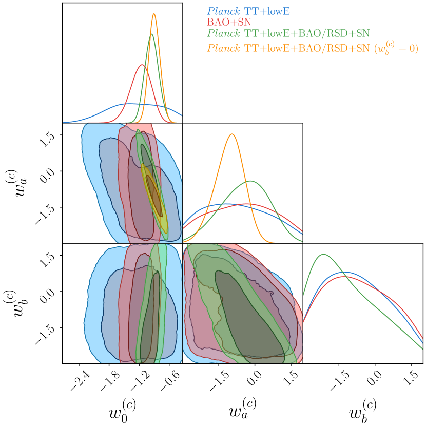
Figure 1: Marginalized posterior distributions for the ($w^{(c)}_{0},w^{(c)}_{a},w^{(c)}_{b}$) parameters of extended CPL model $w(a)_{\rm cpl}=w^{(c)}_{0}+w^{(c)}_{a}(1-a)+w^{(c)}_{b}(1-a)^{2}$. This model does not provide a good fit to the $Planck$ TT+lowE, individually, or in combination with external data. However, the tightest constraints come from the combination $Planck$ TT+lowE+BAO/RSD+SN. The best and tightest constraint on $w^{(c)}_{0}$ and $w^{(c)}_{a}$ is obtained when $w^{(c)}_{b}=0$, indicated with orange contour.

The most trivial generalization for dark energy with a constant equation of state $w_{0}$ is

$$w(a)_{\rm cpl}=w^{(c)}_{0}+w^{(c)}_{a}(1-a),$$ (3)

where in the literature is known as Chevallier–Polarski–Linder (CPL) parameterization (Chevallier & Polarski, 2001; Linder, 2003). At the high redshift equation of state is $w^{(c)}_{0}+w^{(c)}_{a}$ and at the low redshift becomes $w^{(c)}_{0}$, so $w^{(c)}_{0}$ is anticorrelated with $w^{(c)}_{a}$. The simple generalization of CPL equation of state is

$$w(a)_{\rm cpl}=w^{(c)}_{0}+w^{(c)}_{a}(1-a)+w^{(c)}_{b}(1-a)^{2}.$$ (4)

We use priors $-3\leq w^{(c)}_{0}\leq-0.33$, $-3\leq w^{(c)}_{a}\leq 2$, and $-3\leq w^{(c)}_{b}\leq 2$ alongside hard prior $w^{(c)}_{0}+w^{(c)}_{a}+w^{(c)}_{b}\leq 0$ to demand that equation of state remains negative. Marginalized contour of the posterior distributions for $(w^{(c)}_{0},w^{(c)}_{a},w^{(c)}_{b})$ are shown in Fig. 1. A wide volume of parameter space for the equation of state is allowed for both $Planck$ and external data. Adding external data to $Planck$ provides almost the tightest constraints. We obtain

$$\left.\begin{aligned} w^{(c)}_{0}&=-0.95\pm 0.14,\\ w^{(c)}_{a}&=-0.18^{+0.88}_{-1.17},\\ w^{(c)}_{b}&=-2.14^{+1.78}_{-0.78},\end{aligned}\ \right\}\ \ \mbox{\text{\parbox{119.50148pt}{\begin{flushleft}(68\,\% CL, $Planck$ TT+lowE\\ +BAO/RSD+SN),\end{flushleft}}}}$$ (5)

which means the parameters $(w^{(c)}_{0},w^{(c)}_{a},w^{(c)}_{b})$ lie $0.3$, $0.2$ and $1.2\sigma$ away from $(-1,0,0)$. Constraints on both $w^{(c)}_{a}$ and $w^{(c)}_{b}$ are poor from each data set. $Planck$ TT+lowE make $w^{(c)}_{a}$ and $w^{(c)}_{b}$ lie $0.7\sigma$ and $0.8\sigma$ away from zero. When external data are added, the mean values of $w^{(c)}_{a}$ and $w^{(c)}_{b}$ change remarkably, and error bars of $w^{(c)}_{a}$ and $w^{(c)}_{b}$ are respectively reduced by $48\%$ and $45\%$. Fixing $w^{(c)}_{b}=0$, we obtain the constraints

$$\left.\begin{aligned} w^{(c)}_{0}&=-0.91^{+0.12}_{-0.11},\\ w^{(c)}_{a}&=-0.94^{+0.55}_{-0.66},\end{aligned}\ \right\}\ \ \mbox{\text{\parbox{119.50148pt}{\begin{flushleft}(68\,\% CL, $Planck$ TT+lowE\\ +BAO/RSD+SN),\end{flushleft}}}}$$ (6)

which imply that $w^{(c)}_{0}$ and $w^{(c)}_{a}$ lie $0.9$ and $1.7\sigma$ away from $-1$ and zero, respectively. Error bars of $w^{(c)}_{a}$ are decreased by $55\%$ and $78\%$ for the upper and lower bound, respectively. Seljak et al. (2005) obtained $w^{(c)}_{0}=-0.98\pm 0.19$ and $w^{(c)}_{a}={-0.05}^{+0.83}_{-0.65}$ of CPL parameterization for 1st year WMAP+SN measurements in combination with Ly$\alpha$ forest analysis of SDSS. Their results show that CPL is not different from $\Lambda$CDM. We find that at the $1\sigma$ confidence level, the CPL model is not similar to $\Lambda$CDM cosmology for combination $Planck$ TT+lowE+BAO/RSD+SN.

The Bayes factor $\ln B$ is $-0.8$ and $-0.6$ for CPL and extended form $w(a)=w_{0}+w_{a}(1-a)+w_{b}(1-a)^{2}$ with respect to $\Lambda$CDM for full data, respectively. These values for the Bayes factor imply that there is no significant preference for $\Lambda$ dark energy over CPL and its extended form.

3.2 PADE Parametrization

Instead of expressing equation of state $w(a)_{\rm cpl}=w^{(c)}_{0}+w^{(c)}_{a}(1-a)$ up to quadratic expansion, one can parameterize it as

$$w(a)_{\rm pade}=\frac{w^{(p)}_{0}+w^{(p)}_{a}(1-a)}{1+w^{(p)}_{b}(1-a)},$$ (7)

where is named PADE parameterization (Rezaei et al., 2017). At the high redshifts equation of state is $(w^{(p)}_{0}+w^{(p)}_{a})/(1+w^{(p)}_{b})$, and at the low redshifts turns to $w^{(p)}_{0}$. Therefore, $w^{(p)}_{0}$ is anticorrelated with both $w^{(p)}_{a}$ and $w^{(p)}_{b}$. Also, $w^{(p)}_{a}$ and $w^{(p)}_{b}$ are positively correlated. We use priors $-3\leq w^{(p)}_{0}\leq-0.33$ and $-3\leq w^{(p)}_{a}\leq 2$ with $-1\leq w^{(p)}_{b}\leq 2$alongside hard prior $w^{(p)}_{0}+w^{(p)}_{a}\leq 0$ to ensure that equation of state remains non-singular and negative. Marginalized contour of the posterior distributions for $(w^{(p)}_{0},w^{(p)}_{a},w^{(p)}_{b})$ are shown in Fig. 2. We find

$$\left.\begin{aligned} w^{(p)}_{0}&=-0.73^{+0.26}_{-0.32},\\ w^{(p)}_{a}&=-1.07^{+0.58}_{-0.68},\\ w^{(p)}_{b}&=-0.06\pm 0.18,\end{aligned}\ \right\}\ \ \mbox{\text{\parbox{119.50148pt}{\begin{flushleft}(68\,\% CL, $Planck$ TT+lowE\\ +BAO/RSD+SN),\end{flushleft}}}}$$ (8)

which shows the parameters $(w^{(p)}_{0},w^{(p)}_{a},w^{(p)}_{b})$ lie $0.8$, $1.8$ and $0.3\sigma$ away from $(-1,0,0)$ and implies that PADE parameterization at the $1\sigma$ confidence level behaves like CPL parameterization in favour of full data. The parameter $w^{(p)}_{b}$ imposes poor constraints on the $w^{(p)}_{0}$ with respect to $w^{(c)}_{0}$ and pushes $w^{(p)}_{a}$ somewhat to lower value in comparison with $w^{(c)}_{a}$ without change on the error bars (see equation (6)).

Fig. 2 implies that there could exist a tension between CMB and non-CMB data sets, which means one must care to combine them for PADE model. In Bayesian inference, the $R$ statistic provides a measure for clarification tension between two different data sets (Marshall et al., 2006). Given two different independent data sets $A$ and $B$, the Bayesian ratio $R$ is defined via

$$R=\frac{\mathcal{Z}_{A+B}}{\mathcal{Z}_{A}\mathcal{Z}_{B}},$$ (9)

where evidence or marginal likelihood $\mathcal{Z}_{D}$, defined as the probability of measuring the observed data $D$ for a given model $\mathcal{M}$ is given by

$$\mathcal{Z}_{D}\equiv P(D|\mathcal{M})=\int{P(D|\theta,\mathcal{M})~{}P(\theta|\mathcal{M})~{}d\theta}=\int{\mathcal{L}_{D}~{}\pi~{}d\theta}.$$ (10)

Here, $\mathcal{L}_{D}\equiv P(D|\theta,\mathcal{M})$ is the likelihood and $\pi\equiv P(\theta|\mathcal{M})$ denotes prior of parameters $\theta$. The value $R\gg 1$ implies that both data sets are in agreement, while $R\ll 1$ means that data sets are discordant. The $R$ statistic depends on the volume of prior $\pi$, and the tension can be hidden by increasing the prior width (DES Collaboration, 2021). Nevertheless, if $R$ indicates that two data sets are discordant, it should be taken seriously, because increasing the prior width pushes $R$ to the larger value which means two data sets are in agreement (Handley & Lemos, 2019). For these roughly wide priors, $R$ is

$$\ln R=\ln\mathcal{Z}_{Planck+ext}-\ln\mathcal{Z}_{Planck}-\ln\mathcal{Z}_{ext}=-4.17,$$ (11)

where “$ext$” denotes geometrical data. The value $R=0.015$ indicates that PADE dark energy model gives rise to a tension between $Planck$ and geometrical data. Thus, it is better that the PADE model not be considered a reliable parameterization. This tension indicates this model is not favoured by the data.

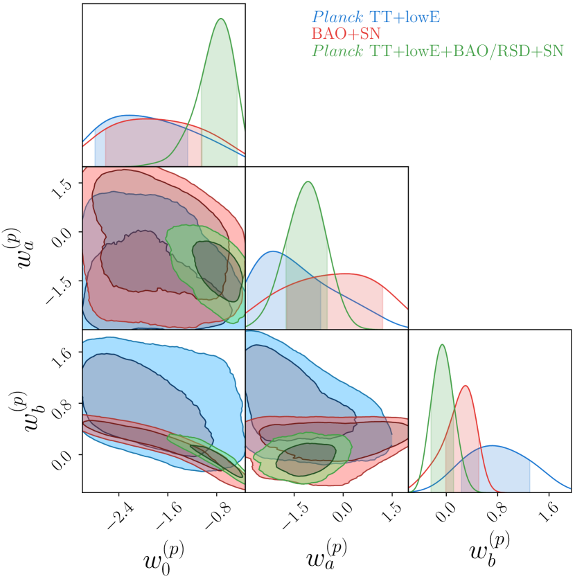
Figure 2: Marginalized posterior distributions for ($w^{(p)}_{0},w^{(p)}_{a},w^{(p)}_{b}$) parameters of the PADE model $w(a)_{\rm pade}={[w^{(p)}_{0}+w^{(p)}_{a}(1-a)]}/{[1+w^{(p)}_{b}(1-a)]}$. $Planck$ TT+lowE provides poor constraints on the dark energy parameters. The $R$ statistic with value $R=0.015$ implies that the $Planck$ CMB and geometrical data are discordant when applied to PADE model. Therefore, the constraints given by equation (8) are not reliable because two data sets must not be combined.

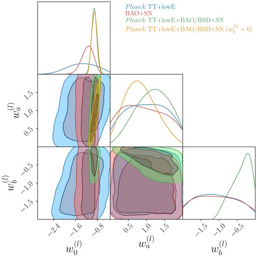
Figure 3: Marginalized posterior distributions of the ($w^{(l)}_{0},w^{(l)}_{a},w^{(l)}_{b}$) parameters for logarithmic model $w(a)_{\rm log}=[{w^{(l)}_{0}+w^{(l)}_{a}\ln a}]/[{1+w^{(l)}_{b}\ln a}]$ from various data. Using $Planck$ TT+lowE alone provides poor constraints with a wide area in parameter space. The tightest constraints come from the combination $Planck$ TT+lowE+BAO/RSD+SN. The orange contour corresponds to $w^{(l)}_{b}=0$, but as we can see the constraints in the plane ($w^{(l)}_{0}$,$w^{(l)}_{a}$) do not change significantly.

3.3 Logarithmic Parametrization

Since the time scale of the expansion history of the Universe is given by $H^{-1}={\left(d\ln a/dt\right)}^{-1}$, following Efstathiou (1999), is worth considering the time scale evolution of dark energy in units of the e-folding scale $\ln a$

$$w(a)_{\rm log}=w^{(l)}_{0}+w^{(l)}_{a}\ln a,$$ (12)

with extended form

$$w(a)_{\rm log}=\frac{w^{(l)}_{0}+w^{(l)}_{a}\ln a}{1+w^{(l)}_{b}\ln a}.$$ (13)

In order that the equation of state remains negative and non-singular, prior of the parameters $w^{(l)}_{a}$ and $w^{(l)}_{b}$ must be chosen positive and negative, respectively. Therefore, $w^{(l)}_{0}$ with both $w^{(l)}_{a}$ and $w^{(l)}_{b}$ is positively correlated, and ($w^{(l)}_{a}$,$w^{(l)}_{b}$) are anti-correlated. We apply priors $-3\leq w^{(l)}_{0}\leq-0.33$, $0\leq w^{(l)}_{a}\leq 2$, and $-2\leq w^{(l)}_{b}\leq 0$. Marginalized contour of the posterior distributions for $(w^{(l)}_{0},w^{(l)}_{a},w^{(l)}_{b})$ are shown in Fig. 3. A wide volume of parameter space for the equation of state is allowed for both $Planck$ and non-CMB data. Geometrical data provides tighter constraints than $Planck$ for $w^{(l)}_{0}$, but both data set impose poor constraints on $w^{(l)}_{a}$ and $w^{(l)}_{b}$. Combining these two data sets provides the tightest constraints with the values

$$\left.\begin{aligned} w^{(l)}_{0}&=-0.92^{+0.09}_{-0.10},\\ w^{(l)}_{a}&=1.23\pm 0.50,\\ w^{(l)}_{b}&=-0.20^{+0.17}_{-0.35},\end{aligned}\ \right\}\ \ \mbox{\text{\parbox{119.50148pt}{\begin{flushleft}(68\,\% CL, $Planck$ TT+lowE\\ +BAO/RSD+SN).\end{flushleft}}}}$$ (14)

Dark energy parameters $(w^{(l)}_{0},w^{(l)}_{a},w^{(l)}_{b})$ lie $1$, $2.8$ and $1.1\sigma$ away from $\Lambda$CDM values. Fixing the parameter $w^{(l)}_{b}=0$, we obtain the constraints

$$\left.\begin{aligned} w^{(l)}_{0}&=-0.91\pm 0.10,\\ w^{(l)}_{a}&=0.74^{+0.48}_{-0.42},\end{aligned}\ \right\}\ \ \mbox{\text{\parbox{119.50148pt}{\begin{flushleft}(68\,\% CL, $Planck$ TT+lowE\\ +BAO/RSD+SN),\end{flushleft}}}}$$ (15)

which implies $w^{(l)}_{0}$ and $w^{(l)}_{a}$ lie $0.9$ and $1.7\sigma$ away from $-1$ and zero, respectively. The parameter $w^{(l)}_{b}$ does not change significantly constraints on $w^{(l)}_{0}$, but pushes the peak of $w^{(l)}_{a}$ to larger value without significant change on the error bars. Staicova & Benisty (2022) obtained $w^{(l)}_{0}=-1.18\pm 0.11$ and $w^{(l)}_{a}=-0.20\pm 0.86$ which means $w^{(l)}_{a}$ lies $0.2\sigma$ away from zero for BAO+SN.

The Bayes factor $\ln B$ is $0.2$ and $-0.8$ for $(w^{(l)}_{0},w^{(l)}_{a})$ and $(w^{(l)}_{0},w^{(l)}_{a},w^{(l)}_{b})$ models with respect to $\Lambda$CDM cosmology for $Planck$ TT+lowE+BAO/RSD+SN, respectively. The values $\ln B=0.2$ and $-0.8$ indicate that the Bayes factor is inconclusive in terms of preference for $w(a)=w_{0}+w_{a}\ln a$ and $\Lambda$ dark energy, respectively.

3.4 Oscillating Parameterization

Number of	Dark energy	Parameters	$\ln B_{w(a)/{\rm{\Lambda}}}$	Outcome
parameters	model		$Planck$ TT+lowE+BAO/RSD+SN
$1$	$\Lambda$	$w_{\Lambda}=-1$	$~{}~{}~{}\cdots$	$\cdots$
	$w_{\rm 0}+w_{a}(1-a)$	$[w_{\rm 0},w_{a}]$	$-0.8$	The preference for $\Lambda$ is inconclusive
2	$w_{\rm 0}+w_{a}\ln a$	$[w_{\rm 0},w_{a}]$	${\color[rgb]{1,1,1}+}0.2$	The preference for $w(a)$ model is inconclusive
	$w_{\rm 0}+w_{a}\sin(\ln a)$	$[w_{\rm 0},w_{a}]$	$-2.0$	The preference for $\Lambda$ is moderate
	$w_{\rm 0}+w_{a}(1-a)+w_{b}(1-a)^{2}$	$[w_{\rm 0},w_{a},w_{b}]$	$-0.6$	The preference for $\Lambda$ is inconclusive
	$\left[{w_{\rm 0}+w_{a}(1-a)}\right]\big{/}{\left[1+w_{b}(1-a)\right]}$	$[w_{\rm 0},w_{a},w_{b}]$	$-2.6~{}(\rm unreliable)$	The $w(a)$ model cannot be compared due to tension
3	$({w_{\rm 0}+w_{a}\ln a})\big{/}({1+w_{b}\ln a})$	$[w_{\rm 0},w_{a},w_{b}]$	$-0.8$	The preference for $\Lambda$ is inconclusive
	$w_{\rm 0}+w_{a}\sin({\mathcal{A}}\ln a)$	$[w_{\rm 0},w_{a},\mathcal{A}]$	$-1.1$	The $w(a)$ model is weakly unsupported

Table 1: Bayesian comparison for time-dependent dark energy models from $Planck$ in combination with external data. Here, the Bayes factor is described as $\ln B_{w(a)/{\rm{\Lambda}}}=\ln{(\mathcal{Z}_{w(a)}/\rm\mathcal{Z}_{{\Lambda}})}$ with $0.4$ as the error on the $\ln B_{w(a)/{\rm{\Lambda}}}$. A negative (positive) value for $\ln B_{w(a)/{\rm{\Lambda}}}$ indicates that the competing model is unsupported (supported) with respect to the $\Lambda$CDM model. For both $w(a)=w_{0}+w_{a}(1-a)$ and $w(a)=w_{0}+w_{a}(1-a)+w_{b}(1-a)^{2}$, the Bayes factor is inconclusive in terms of the preference for $\Lambda$. Nevertheless, the former is the most favourable model because the presence of $w_{b}$ leads to poor constraints on the parameters $w_{0}$ and $w_{a}$. There is no significant support in favour of dark energy $w(a)=w_{0}+w_{a}\ln a$ over $\Lambda$ because this preference is inconclusive. For the equation of state $w(a)=(w_{0}+w_{a}\ln a)/(1+w_{b}\ln a)$, the Bayes factor is inconclusive in terms of preference for $\Lambda$. The model $w(a)=w_{0}+w_{a}\sin(\ln a)$ has the least strength of support where $\Lambda$ dark energy is moderately supported, and the equation of state $w(a)=w_{0}+w_{a}\sin(\mathcal{A}\ln a)$ is weakly unsupported. The Bayesian evidence estimation for model $w(a)=\left[{w_{\rm 0}+w_{a}(1-a)}\right]\big{/}{\left[1+w_{b}(1-a)\right]}$ is not reliable as this model gives rise to a tension between $Planck$ and BAO/RSD+SN when applied for this model, hence, this model cannot be considered as a reliable model.

An oscillating dark energy equation of state can potentially solve coincidence problem (Dodelson et al., 2000; Nojiri & Odintsov, 2006). It is worth mentioning that there is no need to have oscillating potential $V(\varphi)$ for investigating oscillation behavior in the dark energy equation of state $w(a)$ (Linder, 2006). Periodicity of dark energy is described in terms of $\ln a$

$$w(a)_{\rm sin}=w^{(s)}_{0}+w^{(s)}_{a}\sin(\mathcal{A}\ln a+\theta),$$ (16)

because $H^{-1}=(d\ln a/dt)^{-1}$ represents natural period of the cosmic expansion. For the sine function to be injective, we set phase $\theta=0$ to have $-\pi/2\leq\mathcal{A}\ln a\leq 0$ for a wide range of values of the scale factor $a$. The prior $0\leq\mathcal{A}\leq 1$ provides the condition that the sine function is injective for scale factor $a\ll 1$. With a positive $\mathcal{A}$, $w^{(s)}_{0}$ is positively correlated with $w^{(s)}_{a}$ and $\mathcal{A}$. We apply prior $-3\leq w^{(s)}_{0}\leq-0.33$, $0\leq w^{(s)}_{a}\leq 3$ and $0\leq\mathcal{A}\leq 1$. For $\mathcal{A}=1$, we obtain the constraints

$$\left.\begin{aligned} w^{(s)}_{0}&=-0.91^{+0.12}_{-0.10},\\ w^{(s)}_{a}&=0.80^{+0.53}_{-0.47},\end{aligned}\ \right\}\ \ \mbox{\text{\parbox{119.50148pt}{\begin{flushleft}(68\,\% CL, $Planck$ TT+lowE\\ +BAO/RSD+SN),\end{flushleft}}}}$$ (17)

which indicates that $w^{(s)}_{0}$ and $w^{(s)}_{a}$ lie $0.9$ and $1.7\sigma$ away from $\Lambda$CDM values, respectively. Pan et al. (2018) obtained $w^{(s)}_{0}=-0.98\pm 0.05$ and $w^{(s)}_{a}=0.01\pm 0.03$ for $Planck$ (2015)+BAO/RSD+SN. These results show that this model is similar to $\Lambda$CDM because $w^{(s)}_{0}$ and $w^{(s)}_{a}$ are different from -1 and zero at the $0.4$ and $0.3\sigma$ confidence level, respectively. For $\mathcal{A}\neq 1$, $Planck$ data shift the peak of the posterior distribution of $\mathcal{A}$ toward zero value. Adding external data changes significantly constraints on the $w^{(s)}_{0}$ but has no major impact on the posterior of both $w^{(s)}_{a}$ and $\mathcal{A}$. For the full data set, we obtain

$$\left.\begin{aligned} w^{(s)}_{0}&=-0.95^{+0.07}_{-0.08},\\ w^{(s)}_{a}&=1.29^{+0.97}_{-0.69},\\ \mathcal{A}&=0.38^{+0.32}_{-0.21},\end{aligned}\ \right\}\ \ \mbox{\text{\parbox{119.50148pt}{\begin{flushleft}(68\,\% CL, $Planck$ TT+lowE\\ +BAO/RSD+SN),\end{flushleft}}}}$$ (18)

which means dark energy parameters $(w^{(s)}_{0},w^{(s)}_{a},\mathcal{A})$ lie $0.6$, $1.9$ and $1.9\sigma$ away from $(-1,0,1)$. Marginalized contour of the posterior distributions for $(w^{(o)}_{0},w^{(o)}_{a},\mathcal{A})$ are shown in Fig. 4. A varying amplitude $\mathcal{A}$ changes significantly constraints on $w^{(s)}_{0}$ and $w^{(s)}_{a}$. The constraints on $w^{(s)}_{0}$ get somewhat improved and the center is pushed to -1. The peak of posterior distributions of $w^{(o)}_{a}$ moves toward to larger value and error bars are increased by $80\%$ for the upper band for $Planck$ TT+lowE+BAO/RSD+SN. When we only apply $Planck$ measurements, the Hubble parameter $H_{0}$ turns to the high value corresponding to the phantom region as a result of priors of the equation of state parameters.

The Bayes factor $\ln B$ is $-2.0$ and $-1.1$ for $(w^{(s)}_{0},w^{(s)}_{a})$ and $(w^{(s)}_{0},w^{(s)}_{a},\mathcal{A})$ models with respect to $\Lambda$CDM cosmology for $Planck$ TT+lowE+BAO/RSD+SN, respectively. These results show that the strength of support for $\Lambda$ dark energy over $w(a)=w_{0}+w_{a}\sin(\ln a)$ is moderate, and the preference for $\Lambda$ over equation of state $w(a)=w_{0}+w_{a}\sin(\mathcal{A}\ln a)$ is weak.

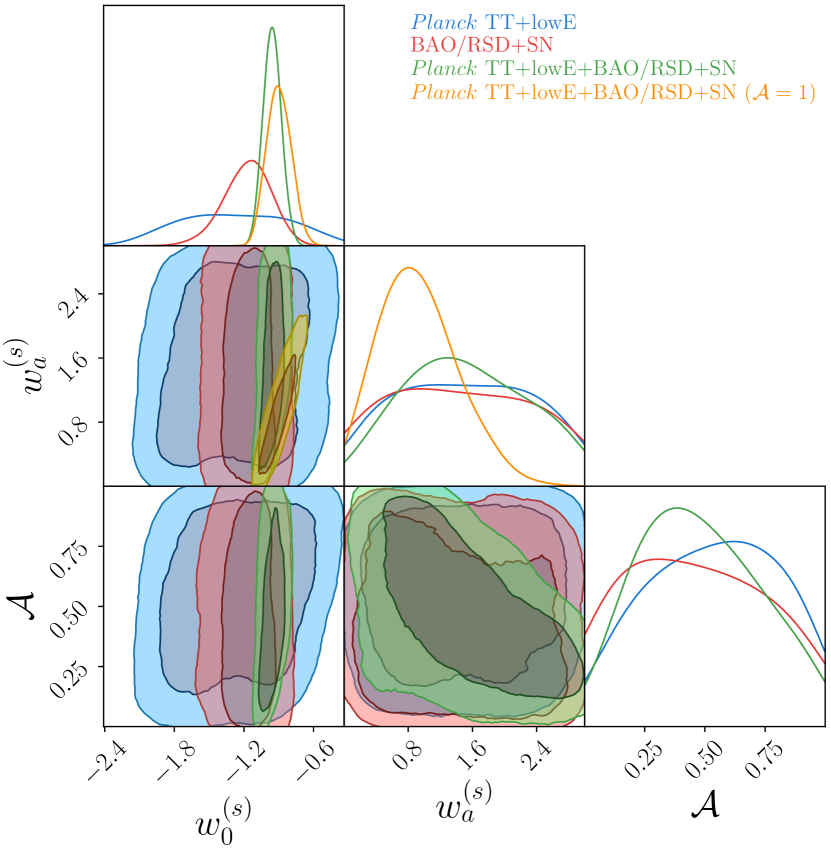
Figure 4: Marginalized posterior distributions of the ($w^{(s)}_{0},w^{(s)}_{a},\mathcal{A}$) parameters for oscillating parameterization $w(a)_{\rm sin}=w^{(s)}_{0}+w^{(s)}_{a}\sin(\mathcal{A}\ln a)$ from various data. The tightest constraints come from the combination $Planck$ TT+lowE+BAO/RSD+SN. Using $Planck$ TT+lowE alone provides poor constraints with a wide area in parameter space that corresponds to large values of the Hubble parameter. The orange contour corresponds to the two free parameters model with $\mathcal{A}=1$, which obviously shows the best and tightest constraints on the $w^{(s)}_{a}$.

4 Discussion & Conclusion

In this work, we imposed observational constraints and performed a model selection approach on the different models of time-dependent dark energy models in favour of $Planck$ temperature and polarization data alongside probes based on distance measurements in combination with RSD measurements. We considered models with two free parameters and then generalize each model to three free parameters in the equation of state. For all models, $Planck$ TT+lowE and non-CMB probes separately provide poor constraints on the parameters and combining them gives rise to the tightest posterior distributions.

Instead of expanding scale factor up to quadratic term $(1-a)^{2}$, we used PADE model $w(a)=[w_{0}+w_{a}(1-a)]/[1+w_{b}(1-a)]$. The $R$ statistic as tension metric indicates that the PADE model gives rise to a tension between $Planck$ CMB measurements and a combination of BAO/RSD+SN which translates into a requirement that there is a problem with the PADE parameterization and it cannot be considered as a reliable model.

We have summarized the Bayes factor for all considered models in Table 1 for full data, in which we quote $0.4$ as the error on the $\ln B_{w(a)/{\rm{\Lambda}}}$. According to the values of the Bayes factor and considering the dispersion of posterior distributions of dark energy free parameters, two-parameter models are sufficient for investigating the time dependency behavior of dark energy, compared to their three free parameter parameterizations. Among models with two free parameters, only logarithmic model $w(a)=w_{0}+w_{a}\ln a$ has a preference over $\Lambda$ dark energy but this strength of support is not significant because $\ln B_{w(a)/{\rm{\Lambda}}}=0.2$. The preference for $\Lambda$ over CPL model $w(a)=w_{0}+w_{a}(1-a)$ is inconclusive with $\ln B_{w(a)/{\rm{\Lambda}}}=-0.8$, and oscillating dark energy $w(a)=w_{0}+w_{a}\sin(\ln a)$ is almost moderately unsupported with respect to $\rm\Lambda CDM$ with $\ln B_{w(a)/{\rm{\Lambda}}}=-2.0$.

For the competing models with three free parameters, the Bayesian evidence implies that the strength of support for $\Lambda$ dark energy over both equations of states $w(a)=w_{0}+w_{a}(1-a)+w_{b}(1-a)^{2}$ and $w(a)=[w_{0}+w_{a}\ln a]/[1+w_{b}\ln a]$ is inconclusive with receptively $\ln B_{w(a)/{\rm{\Lambda}}}=-0.6$ and $-0.8$, and time-dependent dark energy $w(a)=w_{0}+w_{a}\sin(\mathcal{A}\ln a)$ is weakly unsupported with respect to $\rm\Lambda CDM$ with $\ln B_{w(a)/{\rm{\Lambda}}}=-1.1$.

5 acknowledgment

We deeply thank the referee for valuable comments and feedback. The analysis for this paper was run on the Gavazang cluster of the Institute for Advanced Studies in Basic Sciences (IASBS). Also, We are grateful to Bj$\ddot{\rm o}$rn Malte Sch$\ddot{\rm a}$fer for constructive comments.

6 Data Availability

All data used in this work are publicly available and implemented to public package $\tt CosmoSIS$. $Planck$ CMB angular anisotropies power spectra are available from Planck Legacy Archive https://pla.esac.esa.int/#cosmology. The BAO measurements are available from the cited papers, and the Pantheon supernovae data sets are available from https://github.com/dscolnic/Pantheon.

References

- Alam et al. (2017) Alam S., et al., 2017, MNRAS, 470, 2617
- Anderson et al. (2014a) Anderson L., et al., 2014a, MNRAS, 439, 83
- Anderson et al. (2014b) Anderson L., et al., 2014b, MNRAS, 441, 24
- Ata et al. (2018) Ata M., et al., 2018, MNRAS, 473, 4773
- Audren et al. (2013) Audren B., Lesgourgues J., Benabed K., Prunet S., 2013, J. Cosmology Astropart. Phys., 2013, 001
- Ballesteros et al. (2012) Ballesteros G., Hollenstein L., Jain R. K., Kunz M., 2012, J. Cosmology Astropart. Phys., 2012, 038
- Bertschinger (2006) Bertschinger E., 2006, ApJ, 648, 797
- Beutler et al. (2011) Beutler F., et al., 2011, MNRAS, 416, 3017
- Blas et al. (2011) Blas D., Lesgourgues J., Tram T., 2011, J. Cosmology Astropart. Phys., 2011, 034
- Blomqvist et al. (2019) Blomqvist M., et al., 2019, A&A, 629, A86
- Caldwell (2002) Caldwell R. R., 2002, Physics Letters B, 545, 23
- Caldwell et al. (1998) Caldwell R. R., Dave R., Steinhardt P. J., 1998, Phys. Rev. Lett., 80, 1582
- Chevallier & Polarski (2001) Chevallier M., Polarski D., 2001, International Journal of Modern Physics D, 10, 213
- DES Collaboration (2018) DES Collaboration 2018, Phys. Rev. D, 98, 043526
- DES Collaboration (2021) DES Collaboration 2021, MNRAS, 505, 6179
- DES Collaboration (2022) DES Collaboration 2022, arXiv e-prints, p. arXiv:2202.08233
- Dodelson et al. (2000) Dodelson S., Kaplinghat M., Stewart E., 2000, Phys. Rev. Lett., 85, 5276
- Efstathiou (1999) Efstathiou G., 1999, MNRAS, 310, 842
- Einstein (1917) Einstein A., 1917, Sitzungsberichte der Königlich Preußischen Akademie der Wissenschaften (Berlin), pp 142–152
- Eisenstein et al. (1998) Eisenstein D. J., Hu W., Tegmark M., 1998, ApJ, 504, L57
- Fang et al. (2008) Fang W., Hu W., Lewis A., 2008, Phys. Rev. D, 78, 087303
- Feroz et al. (2009) Feroz F., Hobson M. P., Bridges M., 2009, MNRAS, 398, 1601
- Feroz et al. (2019) Feroz F., Hobson M. P., Cameron E., Pettitt A. N., 2019, The Open Journal of Astrophysics, 2, 10
- Handley & Lemos (2019) Handley W., Lemos P., 2019, Phys. Rev. D, 100, 043504
- Hinton (2016) Hinton S. R., 2016, The Journal of Open Source Software, 1, 00045
- Hu (2005) Hu W., 2005, Phys. Rev. D, 71, 047301
- Jassal et al. (2005) Jassal H. K., Bagla J. S., Padmanabhan T., 2005, MNRAS, 356, L11
- Jeffreys (1939) Jeffreys H., 1939, Theory of Probability, Oxford University Press, Oxford
- Kazin et al. (2014) Kazin E. A., et al., 2014, MNRAS, 441, 3524
- Kunz (2012) Kunz M., 2012, Comptes Rendus Physique, 13, 539
- Lewis & Bridle (2002) Lewis A., Bridle S., 2002, Phys. Rev. D, 66, 103511
- Lewis et al. (2000) Lewis A., Challinor A., Lasenby A., 2000, ApJ, 538, 473
- Linder (2003) Linder E. V., 2003, Phys. Rev. Lett., 90, 091301
- Linder (2005) Linder E. V., 2005, Phys. Rev. D, 72, 043529
- Linder (2006) Linder E. V., 2006, Astroparticle Physics, 25, 167
- Maor et al. (2001) Maor I., Brustein R., Steinhardt P. J., 2001, Phys. Rev. Lett., 86, 6
- Marshall et al. (2006) Marshall P., Rajguru N., Slosar A., 2006, Phys. Rev. D, 73, 067302
- Mehta et al. (2012) Mehta K. T., Cuesta A. J., Xu X., Eisenstein D. J., Padmanabhan N., 2012, MNRAS, 427, 2168
- Nojiri & Odintsov (2006) Nojiri S., Odintsov S. D., 2006, Physics Letters B, 637, 139
- Pan et al. (2018) Pan S., Saridakis E. N., Yang W., 2018, Phys. Rev. D, 98, 063510
- Percival & White (2009) Percival W. J., White M., 2009, MNRAS, 393, 297
- Perlmutter et al. (1998) Perlmutter S., et al., 1998, Nature, 391, 51
- Planck Collaboration V (2020) Planck Collaboration V 2020, A&A, 641, A5
- Planck Collaboration VI (2020) Planck Collaboration VI 2020, A&A, 641, A6
- Planck Collaboration XIV (2016) Planck Collaboration XIV 2016, A&A, 594, A14
- Ratra & Peebles (1988) Ratra B., Peebles P. J. E., 1988, Phys. Rev. D, 37, 3406
- Rezaei et al. (2017) Rezaei M., Malekjani M., Basilakos S., Mehrabi A., Mota D. F., 2017, ApJ, 843, 65
- Riess et al. (1998) Riess A. G., et al., 1998, AJ, 116, 1009
- Riess et al. (2004) Riess A. G., et al., 2004, ApJ, 607, 665
- Ross et al. (2015) Ross A. J., Samushia L., Howlett C., Percival W. J., Burden A., Manera M., 2015, MNRAS, 449, 835
- Scolnic et al. (2018) Scolnic D. M., et al., 2018, ApJ, 859, 101
- Seljak et al. (2005) Seljak U., et al., 2005, Phys. Rev. D, 71, 103515
- Staicova & Benisty (2022) Staicova D., Benisty D., 2022, A&A, 668, A135
- Trotta (2007) Trotta R., 2007, MNRAS, 378, 72
- Vikman (2005) Vikman A., 2005, Phys. Rev. D, 71, 023515
- Weinberg (1989) Weinberg S., 1989, Reviews of Modern Physics, 61, 1
- Wetterich (1988) Wetterich C., 1988, Nuclear Physics B, 302, 668
- Xia et al. (2006) Xia J.-Q., Zhao G.-B., Li H., Feng B., Zhang X., 2006, Phys. Rev. D, 74, 083521
- Zuntz et al. (2015) Zuntz J., et al., 2015, Astronomy and Computing, 12, 45