Decouple Graph Neural Networks: Train Multiple Simple GNNs Simultaneously Instead of One

Abstract

Graph neural networks (GNN) suffer from severe inefficiency due to the exponential growth of node dependency with the increase of layers. It extremely limits the application of stochastic optimization algorithms so that the training of GNN is usually time-consuming. To address this problem, we propose to decouple a multi-layer GNN as multiple simple modules for more efficient training, which is comprised of classical forward training (FT) and designed backward training (BT). Under the proposed framework, each module can be trained efficiently in FT by stochastic algorithms without distortion of graph information owing to its simplicity. To avoid the only unidirectional information delivery of FT and sufficiently train shallow modules with the deeper ones, we develop a backward training mechanism that makes the former modules perceive the latter modules, inspired by the classical backward propagation algorithm. The backward training introduces the reversed information delivery into the decoupled modules as well as the forward information delivery. To investigate how the decoupling and greedy training affect the representational capacity, we theoretically prove that the error produced by linear modules will not accumulate on unsupervised tasks in most cases. The theoretical and experimental results show that the proposed framework is highly efficient with reasonable performance, which may deserve more investigation.

1 Introduction

In recent years, neural networks [1, 2], due to the impressive performance, have been extended to graph data, known as graph neural networks (GNN) [3]. As GNNs significantly improve the results of graph tasks, it has been extensively investigated from different aspects, such as graph convolution network (GCN) [4, 5], graph attention networks (GAT) [6, 7], spatial-temporal GNN (STGNN) [8], graph auto-encoder [9, 10], graph contrastive learning [11], etc.

Except for the variants that originate from different perspectives, an important topic is motivated by the well-known inefficiency of GNN. In classical neural networks [2], the optimization is usually based on stochastic algorithms with limited batch [12, 13] since samples are independent of each other. However, the aggregation-like operations defined in [14] result in the dependency of each node on its neighbors and the amount of dependent nodes for one node increases exponentially with the growth of layers, which results in the unexpected increases of batch size. Some works are proposed based on neighbor sampling [14, 15, 16, 17] and graph approximation [18] to limit the batch size, while some methods [19, 20] attempt to directly apply high-order graph operation and sacrifice the most non-linearity. The training stability is a problem for neighbor sampling methods [14, 15, 17] though VRGCN [16] has attempted to control the variance via improving sampling. Note that the required nodes may still grow (slowly) with the increase of depth. ClusterGCN [18] finds an approximate graph with plenty of connected components so that the batch size is strictly upper-bounded. The major challenge of these methods is the information missing during sampling. The simplified methods [19, 20] are efficient but the limited non-linearity may be the bottleneck of these methods. These methods may incorporate the idea of GIN [21] to improve the capacity [20].

To apply stochastic optimization while retaining the exact graph structure, we propose a framework, namely stacked graph neural network (SGNN), which decouples a multi-layer GNN as multiple simple GNN modules and then trains them simultaneously rather than connecting them with the increase of the depth. Inspired by the backward propagation algorithm, we find that the main difference between stacked networks [22] and classical networks is no training information propagated from the latter modules to the former ones. The lack of backward information delivery may be the main reason of the performance limitation of stacked models. The contributions are concluded as: (1) We accordingly propose a backward training strategy to let the former modules receive the information from the final loss and latter modules, which leads to a cycled training framework to control bias and train shallow modules correctly. (2) Under this framework, a multi-layer GNN can be decoupled into multiple simple GNNs, named as separable GNNs in this paper, so that every training step could use the stochastic optimization without any samplings or changes on graph. Therefore, SGNN could take both non-linearity and high efficiency into account. (3) We investigate how the decoupling and greedy training affect the representational capacity of the linear SGNN. It is proved that the error would not accumulate in most cases when the final objective is graph reconstruction.

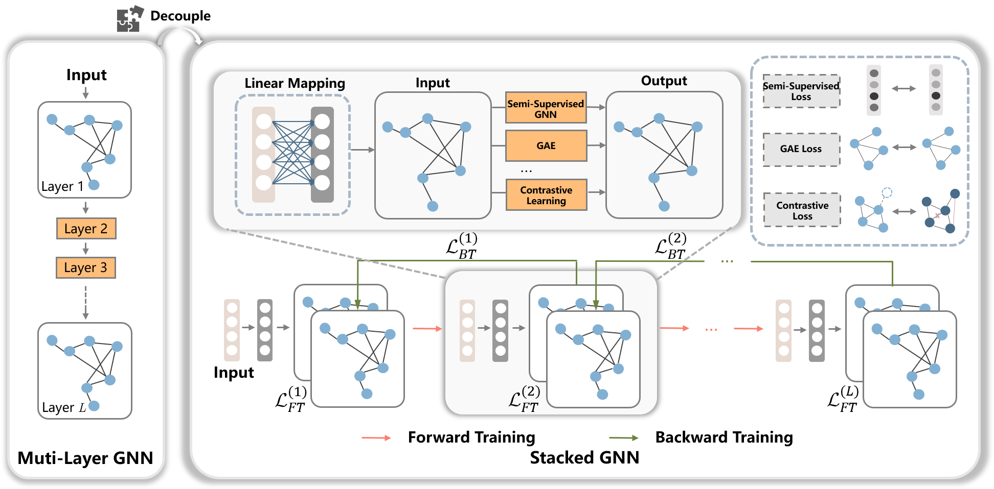
Figure 1: Illustration of a stacked graph neural network decoupled from an $L$-layer GNN. To train each module individually, some loss (e.g., semi-supervised loss, unsupervised loss, contrastive loss) is required and it is denoted by $\mathcal{L}_{FT}^{(t)}$. To let the shallow modules perceive the deeper ones, $\mathcal{M}_{t}$ passes back the expected input features to $\mathcal{M}_{t-1}$ during the backward training. The divergence between the features output by $\mathcal{M}_{t}$ and the expected features of $\mathcal{M}_{t-1}$ formulates the BT loss $\mathcal{L}_{BT}^{(t)}$.

2 Background

Graph Neural Networks Aiming to extend convolution operation into graph, graph convolution became a hot topic [5, 23, 24] and graph convolution network (GCN) [4] has become an important baseline. By introducing self-attention techniques [25], graph attention networks (GAT) [6, 7] are proposed and applied to other applications [26, 27]. As [28] claimed that GNNs suffer from the over-smoothing problem, GALA [10] develops the graph sharpening and ResGCN [29] attempts to designs a deeper architecture. The theoretical works [28, 30, 31] have different views towards the depth of GNNs. Some works [28, 30] claimed that the expressive power of GNN decreases with the increase of layers, while the others argue that the assumptions in [30] may not hold and deeper GNNs have stronger power [31]. Moreover, some works [32, 21] investigate the expressive capability by showing the connection between Weisfeiler-Lehman test [33] and GNNs. Nevertheless, most of them neglect the inefficiency problem of GNNs.

Efficient Graph Neural Networks To accelerate the optimization through batch gradient descent to GNN without too much deviation, several models [14, 15, 16, 17] propose to sample data points according to graph topology. These models propose different sampling strategies to obtain stable results. GraphSAGE [14] produces a subgraph with limited neighbors for each node while FastGCN [15] samples fixed nodes for each layer with the importance sampling. The variance of sampling is further controlled in [16]. ClusterGCN [18] aims to generate an approximate graph with plenty of connected components so that each component can be used as a batch per step. SGC [19] simplifies GCN by setting all activations of middle layers as linear functions and SSGC [20] further improves it. In summary, SGNN proposed in this paper retains the non-linearity and requires no node sampling or sub-graph sampling. L2-GCN [34] attempts to extend the idea of the classical stacked auto-encoder into the popular GCN while DGL-GNN [35] further develops a parallel version. They both fail to train all GNN modules jointly but SGNN firstly offers a novel framework to train them like training layers in a conventional neural network.

Connections to Existing Models Stacked Auto-Encoder (SAE) [22] is a model applied to the pre-training of neural networks. It trains the current two-layer auto-encoder [36] and then feeds the latent features output by the middle layer to the next auto-encoder. The model is often used as a pre-training model instead of a formal model. MGAE [37] is an extension of SAE and its fundamental module is graph auto-encoder [9]. The main difference compared with the proposed model is whether each module could be perceived by modules from both forward and backward directions. The stack paradigm is similar to the classical boosting models [38, 39, 40] while some works [41, 42] also investigated the boosting algorithm of neural networks. In recent years, some boosting GNN models [43, 44] are also developed. The most boosting algorithms (e.g., [41, 43]) aim to learn a prediction function gradually while the proposed SGNN aims to learn ideal embeddings gradually. Note that AdaGCN [44] is also trained gradually and the features are combined using AdaBoost [38]. More importantly, all these boosting methods for GNNs are only trained forward and the backward training is missing. Deep neural interface [45] proposes to decouple neural networks to asynchronously accelerate the computation of gradients. The decoupling is an acceleration trick to compute the gradients of $L$-layer networks, while SGNN proposed in this paper explicitly separates an $L$-layer GNN into $L$ simple modules. In other words, the ultimate goal of SGNN is not to optimize an $L$-layer GNN.

3 Proposed Method

Motivated by SAE [22] and the fact that the simplified models [19, 20] are highly efficient for GNN, we therefore rethink the substantial difference between the stacked networks and multi-layer GNNs. To sum up, we attempt to answer the following two questions in this paper:

• How to decouple a complex GNN into multiple simple GNNs and train them jointly?

• How does the decoupling affect the representational capacity and final performance?

We will discuss the first question in this section and then elaborate on another one in Section 4.

3.1 Preliminary

Each decoupled GNN model of the proposed model is named as a module and the $t$-th module is denoted by $\mathcal{M}_{t}$ for simplicity. The vector and matrix are denoted by lower-case and upper-case letters in bold, respectively. $\|\cdot\|$ represents the Frobenius norm. Given a graph, let $\bm{A}\in\mathbb{R}^{n\times n}$ be adjacency matrix and $\bm{X}\in\mathbb{R}^{n\times d}$ be node features. A typical GNN layer can be usually defined as

$$\bm{H}=f(\bm{A},\bm{X},\bm{W})=\varphi(\bm{P}\bm{X}\bm{W}),$$ (1)

where $\bm{W}$ is projection coefficient and $\bm{P}=\phi(\bm{A})$ is a function of $\bm{A}$. When we discuss each individual module, we assume that $\bm{W}\in\mathbb{R}^{d\times k}$ for simplicity. For example, GCN [4] defines $\bm{P}$ as $\bm{P}_{\rm GCN}=\bm{D}^{-\frac{1}{2}}(\bm{A}+\bm{I})\bm{D}^{-\frac{1}{2}}$ and $\bm{D}$ is the degree matrix of $\bm{A}+\bm{I}$. When multiple layers are integrated, the learned representation given by multiple GNN layers can be written as

$$\begin{split}\bm{H}&=f_{1}\circ f_{2}\circ\cdots\circ f_{L}(\bm{A},\bm{X},\bm{W}_{1},\ldots,\bm{W}_{L})\\ &=\varphi_{L}(\bm{P}\varphi_{L-1}(\cdots\varphi_{1}(\bm{P}\bm{X}\bm{W}_{1})\cdots)\bm{W}_{L}),\end{split}$$ (2)

where $L$ is the amount of layers. Assume that the average number of neighbors is $c$. To compute $\bm{H}$, each sample will need $\mathcal{O}(c^{L})$ extra samples. If the depth is large and the graph is connected, then all nodes have to be engaged to compute for one node. The uncontrolled batch size results in the time-consuming training. In vanilla GNNs, the computational complexity is $\mathcal{O}(KL\|\bm{A}\|_{0}\sum_{i=0}^{m-1}d_{i}d_{i+1})$ on sparse graphs where $K$ is the number of iterations and $d_{i}$ is the dimension of $\bm{W}_{i}$. For large-scale datasets, both time and space complexity are too expensive.

3.2 Stacked Graph Neural Networks

Although the stacked networks usually have more parameters than multi-layer networks, which frequently indicates that the stacked networks may be more powerful, they only serve as a technique for pre-training. Specifically speaking, they simply transfer the representations learned by the current network to the next one but no feedback is passed back. It causes the invisibility of the succeeding modules and the final objective. As a result of the unreliability of the former modules, the stacked model is conventionally used as an unsupervised pre-training model.

Rethinking the learning process of a network, multiple layers are optimized simultaneously by gradient-based methods where the gradient is calculated by the well-known backward propagation algorithm [46]. The algorithm consists of forward propagation (FP) and backward propagation (BP). FP computes the required values for BP, which can be viewed as an information delivery process. Note that FP is similar to the training of the stacked networks. Specifically, transferring the output of the current module to the next one in the stacked network is like the computation of neurons layer by layer during FP. Inspired by this, we aim to design a BP-like training strategy, namely backward training (BT), so that the former modules could be tuned according to the feedback. The core idea of our stacked graph neural network (SGNN) is shown in Figure 1.

3.2.1 Separability: Crucial Concept for Efficiency

Before introducing SGNN in detail, we formally introduce the key concept and core motivation of how to accelerate GNN via SGNN.

Definition 3.1.

If a GNN model can be formulated as $f(\bm{A},\bm{X},\bm{W})=f_{1}(f_{0}(\bm{A},\bm{X}),\bm{W})$, then it is a separable GNN. If it can be further formulated as $f(\bm{A},\bm{X},\bm{W})=f_{1}(f_{0}(\bm{A},\bm{X}),\bm{W})=g_{1}(\bm{A},g_{0}(\bm{X},\bm{W}))$, then it is a fully-separable GNN.

To keep simplicity, define the set of separable GNNs as $\mathcal{F}_{k}=\{f:\mathbb{R}^{n\times n}\times\mathbb{R}^{n\times d}\times\mathbb{R}^{d\times k}\mapsto\mathbb{R}^{n\times k}|f(\bm{A},\bm{X},\bm{W})=f_{1}(f_{0}(\bm{A},\bm{X}),\bm{W})\}$ and the set of fully-separable GNNs as $\mathcal{F}_{k}^{*}=\{f:\mathbb{R}^{n\times n}\times\mathbb{R}^{n\times d}\times\mathbb{R}^{d\times k}\mapsto\mathbb{R}|f(\bm{A},\bm{X},\bm{W})=f_{1}(f_{0}(\bm{A},\bm{X}),\bm{W})=g_{1}(\bm{A},g_{0}(\bm{X},\bm{W}))\}$. Note that most single-layer GNN models are fully-separable. For instance, SGC [19] is fully-separable where $f_{0}(\bm{A},\bm{X})=\bm{P}^{m}\bm{X}$ and $f_{1}(f_{0}(\bm{A},\bm{X}),\bm{W})=\varphi(f_{0}(\bm{A},\bm{X})\cdot\bm{W})$, while the single-layer GIN [3] is separable but not fully-separable since $\bm{P}\cdot{\rm MLP}(\bm{X})\neq{\rm MLP}(\bm{PX})$ usually holds. However, a single-layer GAT [6] is not separable since the graph operation is relevant to $\bm{W}$.

The separable property actually factorizes a GNN model to 2 parts, graph operation $f_{0}$ and neural operation $f_{1}$. Since all dependencies among nodes in GNNs are caused by the graph operation, one can compute $\bm{X}^{\prime}=f_{0}(\bm{A},\bm{X})$ once (like preprocessing) in separable GNNs and then the GNN is converted into a typical network. After computing $\bm{X}^{\prime}$, the information contained in graph has been passed into $\bm{X}^{\prime}$ and the succeeding sampling would not affect the topology of graph. Therefore, we can obtain a highly efficient GNN model that can be optimized by SGD, provided that each module is separable. On the other hand, the fully-separable condition is essential for the backward training to pass back the information over multiple modules. Since most single-layer GNNs are separable but not fully-separable, we show how to revise separable GNNs to introduce the fully-separability.

Then, we formally clarify the core idea of SGNN by showing how to handle Q1.

3.2.2 Forward Training (FT)

The first challenge is how to set the training objective for each module $\mathcal{M}_{t}$. It is crucial to apply SGNN to both supervised and unsupervised scenes. Suppose that we have a separable GNN module $\mathcal{M}$ and let $\bm{H}=f(\bm{A},\bm{X},\bm{W})$ be the features learned by the separable GNN module. For the unsupervised cases, if $\mathcal{M}_{t}$ is a GAE, then the loss of FT is formulated as

$$\mathcal{L}_{FT}=\ell(\bm{A},\bm{X},\bm{H})=d(\bm{A},\kappa(\bm{H})),$$ (3)

where $d(\cdot,\cdot)$ represents the metric function and $\kappa:\mathbb{R}^{n\times k}\mapsto\mathbb{R}^{n\times n}$ is a mapping function. For instance, a simple loss introduced by [9] is $d(\bm{A},\kappa(H))=KL(\bm{A}\|\sigma(\bm{H}\bm{H}^{T}))$ where $\sigma(\cdot)$ is the sigmoid function, and $KL(\cdot\|\cdot)$ is the Kullback-Leibler divergence. The other options include but not limited to symmetric content reconstruction [10] and graph contrastive learning [11]. For modules with supervision information, a projection matrix $\bm{R}\in\mathbb{R}^{k\times c}$ is introduced to map the $k$-dimension embedding vector into soft labels with $c$ classes. For the node classification, the loss can be simply set as

$$\mathcal{L}_{FT}=KL(\bm{Y}\|\textrm{softmax}(\bm{H}\bm{R})),$$ (4)

where $\bm{Y}\in\mathbb{R}^{n\times c}$ is the supervision information for supervised tasks. Note that the above loss is equivalent to the classical softmax regression if $\bm{H}$ is constant. The loss could also be link prediction, graph classification, etc. Although base modules can utilize diverse losses, we only discuss the situation that all modules use the same kind of loss in this paper for simplicity.

Input : Adjacency matrix $\bm{A}$, feature matrix $\bm{X}$, balance coefficient $\eta$, the number of epochs $K$, $L$ separable GNN modules $\{\mathcal{M}_{t}\}_{t=1}^{L}$, $\bm{H}_{0}\leftarrow\bm{X}$.

Output : Features output by $\mathcal{M}_{L}$.

for $i=1,\ldots,K$ do

       # Forward Train Stacked Graph Neural Networks

       for $t=1,2,\ldots,L-1$ do

             Feed the current features to $\mathcal{M}_{t}$ and reset $\bm{U}_{t}$: $\bm{X}_{t}\leftarrow\bm{H}_{t-1}$, $\bm{U}_{t}\leftarrow\bm{I}$.

             # Train with only $\mathcal{L}_{FT}$ at the first forward training

             ${\bm{X}_{t}}^{\prime}=f_{0}^{(t)}(\bm{A},\bm{X}_{t})$    # Preprocessing for mini-batch algorithms

             Compute loss $\mathcal{L}^{(t)}\leftarrow\mathcal{L}_{FT}^{(t)}$ if $i==1$ else $\mathcal{L}_{FT}^{(t)}+\eta\mathcal{L}_{BT}^{(t)}$

             Train $\mathcal{M}_{t}$ by optimizing $\min_{\bm{W}_{t}}\mathcal{L}^{(t)}$ based on mini-batch algorithms.

             Obtain the features: $\bm{H}_{t}\leftarrow f^{(t)}_{1}({\bm{X}_{t}}^{\prime},\bm{W}_{t})$.

      $\bm{X}_{L}\leftarrow\bm{H}_{t}$, $\bm{U}_{L}\leftarrow\bm{I}$, ${\bm{X}}_{L}^{\prime}=f_{0}^{(L)}(\bm{A},X_{L})$.

       Train $\mathcal{M}_{L}$ by optimizing $\min_{\bm{W}_{L},\bm{U}_{L}}\mathcal{L}_{FT}^{(L)}$ based on mini-batch algorithms.

       # Backward Train Stacked Graph Neural Networks

       for $t=L-1,L-2,\ldots,1$ do

             Compute the expected output feature of $\mathcal{M}_{t}$: $\bm{Z}_{t+1}\leftarrow(g^{*}_{0})_{t+1}(\bm{X}_{t+1},\bm{U}_{t+1})$.

             Train $\mathcal{M}_{t}$ by optimizing $\min_{\bm{W}_{t},\bm{U}_{t}}\mathcal{L}_{FT}^{(t)}+\eta\mathcal{L}_{BT}^{(t)}$ based on mini-batch algorithms.

      

Algorithm 1 Procedure of Stacked Graph Neural Networks Composed of $L$ Modules

3.2.3 Backward Training (BT)

The second challenge is how to train multiple separable GNNs simultaneously in order to ensure performance. Roughly speaking, the gradients of all layers in neural networks are computed exactly due to the repeated delivery of information by FP and BP. BP lets the shallow layers perceive the deep ones through the feedback, while the tail modules are invisible to the head ones in FT. We accordingly design the backward training (BT) for SGNN. To achieve the reverse information delivery, a separable GNN layer is modified by introducing the fully-separability,

$$\begin{split}\bm{H}&=\hat{f}(\bm{A},\bm{X},\bm{W})=\hat{f}_{1}(\hat{f}_{0}(\bm{A},\bm{X}),\bm{W})\\ &=\hat{f}_{1}(f^{*}(\bm{A},\bm{X},\bm{U}),\bm{W}),~{}\forall\hat{f}\in\mathcal{F}_{k},f^{*}\in\mathcal{F}_{d}^{*},\end{split}$$ (5)

where $\bm{U}\in\mathbb{R}^{d\times d}$ and $\bm{W}\in\mathbb{R}^{d\times k}$. Note that $f^{*}(\bm{A},\bm{X},\bm{U})=g_{1}^{*}(\bm{A},g_{0}^{*}(\bm{X},\bm{U}))$. Clearly, if $\bm{U}$ is fixed as a constant, then the modified layer is equivalent to the original separable GNN layer $\hat{f}$. Denote $\bm{Z}=g_{0}^{*}(\bm{X},\bm{U})$ and $\bm{Z}$ is the expected features. Specifically, $\bm{Z}_{t}$ is the learned feature during the backward training of $\mathcal{M}_{t}$, and it is also the expected input of $\mathcal{M}_{t}$, i.e., from $\mathcal{M}_{t-1}$. In the forward training, the delivery of information is based on the learned features $\bm{H}_{t}$, and $\bm{Z}$ plays the similar role in the backward training. The loss of backward training attempts to shrink the difference between the output feature $\bm{H}_{t}$ of $\mathcal{M}_{t}$ and expected input $\bm{Z}_{t+1}$ of $\mathcal{M}_{t+1}$,

$$\mathcal{L}_{BT}^{(t)}=d(\bm{H}_{t},\bm{Z}_{t+1})=d(f^{*}_{t}(\bm{A},\bm{X}_{t},\bm{U}_{t}),\bm{Z}_{t+1}).$$ (6)

Note that $\mathcal{L}_{BT}$ is only activated after the first forward training leading to the final loss of $\mathcal{M}_{t}$ as

$$\mathcal{L}^{(t)}=\mathcal{L}_{FT}^{(t)}+\eta\mathcal{L}_{BT}^{(t)},$$ (7)

and it is updated during each backward training. The introduction of $\bm{Z}$ will not limit the application of stochastic optimization since the expected features can also be sampled at each iteration without restrictions. The procedure is summarized as Algorithm 1.

Remark that $\bm{U}_{t}$ remains as the identity matrix during FT. This setting leads to each forward computation across $L$ base modules being equivalent to a forward propagation $L$-layer GNN. In other words, an SGNN with $L$ modules can be regarded as a decomposition of an $L$-layer GNN. One may concern that why not to learn $\bm{U}_{t}$ and $\bm{W}_{t}$ together in FT. In this case, we prefer to use $\bm{U}_{t}$ only for learning the expected features of $\mathcal{M}_{t+1}$ and the capability improvement from the co-learning $\bm{U}_{t}$ in FT could also be implemented by $\bm{W}$, which is equivalent to use GIN [21] as base modules.

3.3 Complexity

As each base module is assumed as a separable GNN, both FT and BT of $\mathcal{M}_{t}$ can be divided into two steps, the preprocessing step for graph operation and the training step for parameters learning. Denote the output dimension of $\mathcal{M}_{t}$ as $d_{t}$ and the dimension of original content feature as $d_{0}=d$. The preprocessing to compute ${\bm{X}}_{t}^{\prime}=f_{0}(\bm{A},\bm{X}_{t})$ requires $\mathcal{O}(\|\bm{A}\|_{0}d_{t})$ cost. Suppose that each module is trained $E$ iterations and the batch size is set as $m$. Then the computation cost of the training step is $\mathcal{O}(Emd_{t-1}d_{t})$. Note that only the GNN mapping is considered and the computation of the loss is ignored. Overall, the computational complexity of an SGNN with $L$ modules is approximately $\mathcal{O}(K\|\bm{A}\|_{0}\sum_{t=0}^{L-1}d_{t}+Em\sum_{t=1}^{L}d_{t-1}d_{t})$. Remark that the graph is only used once during every epoch and no sampling is processed on the graph such that the graph structure is completely retained which is unavailable in the existing fast GNNs. The coefficient of $\|\bm{A}\|_{0}$ is only $K\sum_{t=1}^{L-1}d_{t}$. The space complexity is only $\mathcal{O}(\|\bm{A}\|_{0}+md_{t-1}d_{t})$. Therefore, the growth of graph scale will not affect the efficiency of SGNN. Due to the efficiency, all experiments can be conducted on a PC with an NVIDIA 1660 (6GB) and 16GB RAM.

4 Theoretical Analysis

To answer Q2 raised in the beginning of Section 3, we discuss the impact of the decoupling in this section. Intuitively speaking, if an $L$-layer GNN achieves satisfactory results, then there exists $\{\bm{W}_{t}\}_{t=1}^{L}$ such that an SGNN with $L$ modules could achieve the same results. However, each $\mathcal{M}_{t}$ is trained greedily according to the forward training loss $\mathcal{L}_{FT}$, while middle layers of a multi-layer GNN are trained according to the same objective. The major concern is whether the embedding learned by a greedy strategy leads to an irreversible deviation in the forward training.

In this section, we investigate the possible side effects on a specific SGNN comprised of unsupervised modules defined in Eq. (3) with linear activations. The conclusion is not apparent since simply setting $\bm{W}$ as an identity matrix does not prove it for GNN due to the existence of $\bm{P}$. Remark that a basic premise is that the previous module has achieved a reasonable result.

Given a linear separable-GNN module $\mathcal{M}$ which is defined as $\bm{H}=\bm{PXW}\in\mathbb{R}^{n\times k}$, suppose that the forward training uses the reconstruction error $\|\bm{P}-\bm{H}\bm{H}^{T}\|$ as $\mathcal{L}_{FT}$. We first introduce the matrix angle to better understand whether the preconditions of Theorem 4.1 are practicable.

Definition 4.1.

Given two matrices $\bm{B}_{1},\bm{B}_{2}\in\mathbb{R}^{n\times n}$, we define the matrix angle as $\theta(\bm{B}_{1},\bm{B}_{2})=\arccos\langle\bm{B}_{1},\bm{B}_{2}\rangle/(\|\bm{B}_{1}\|\cdot\|\bm{B}_{2}\|)$.

Before elaborating on theorems, we introduce the following assumption, which separates the discussions into two cases.

Assumption 4.1.

$\bm{X}\bm{X}^{T}$ does not share the same eigenspace with $\bm{P}-\bm{X}\bm{X}^{T}$.

Note that the above assumption is weak and frequently holds in most cases. For simplicity, $\bm{U}_{r}\in\mathbb{R}^{n\times r}$ ($r\in\mathbb{N}_{+}$) is the eigenvectors associated with $r$ leading eigenvalues. Under this assumption, we find that the error of $\mathcal{M}$ is upper-bounded by $\varepsilon$.

Theorem 4.1.

Let $\delta=1-\cos(\theta_{*}/2)$ and $\theta_{*}=\theta((\bm{P}-\bm{X}\bm{X}^{T})\bm{Q},\bm{Q}(\bm{P}-\bm{X}\bm{X}^{T}))$ where $\bm{Q}=\bm{U}_{o}\bm{U}_{o}^{T}-\bm{I}/2$ and $o=\min({\rm rank}(\bm{X}),k)$. Under Assumption 4.1, if $\|\bm{P}-\bm{H}\bm{H}^{T}\|=\varepsilon\leq\mathcal{O}(\delta)$ and $\sigma_{*}\leq\mathcal{O}(\sqrt{\delta})$ where $\sigma_{*}$ is the $(o+1)$-th largest singular value of $\bm{X}$, then there exists $\bm{W}\in\mathbb{R}^{d\times k}$ so that $\|\bm{P}-\bm{H}\bm{H}^{T}\|\leq\varepsilon$. In other words, if $\varepsilon$ is small enough, then $\bm{H}\bm{H}^{T}$ could be a better approximation than $\bm{X}\bm{X}^{T}$.

Specially, if ${\rm rank}(\bm{X})\leq k$ or $k=d$, $\sigma_{*}=0$ so that $\sigma_{*}\leq\mathcal{O}(\sqrt{\delta})$ holds. From the above theorem, we claim that the error through $\mathcal{M}$ will not accumulate (i.e., bound by $\varepsilon$) provided that the input $\bm{X}$, the output of the previous modules, is well-trained. We further provide an upper-bound of error if Assumption 4.1 does not hold. The following theorem shows the increasing speed of error is at most linear with the tail singular-values.

Theorem 4.2.

If Assumption 4.1 does not hold, then there exists $\bm{W}\in\mathbb{R}^{d\times k}$ so that $\|\bm{P}-\bm{H}\bm{H}^{T}\|\leq\varepsilon+\mathcal{O}(\sigma_{*}^{2})$.

Corollary 4.1.

Given an SGNN with $L$ linear modules $\{\mathcal{M}_{t}\}_{t=1}^{L}$ with $\mathcal{L}_{FT}^{(t)}=\|\bm{P}-\bm{H}_{t}\bm{H}_{t}^{T}\|$, if $\bm{P}-\bm{H}_{1}\bm{H}_{1}^{T}$ and $\bm{H}_{1}\bm{H}_{1}^{T}$ share the same eigenspace, then $\mathcal{L}^{(L)}_{FT}\leq\mathcal{L}^{(1)}_{FT}+\sum_{t=1}^{L-1}\mathcal{O}(\sigma_{*}^{2}(\bm{H}_{t}))$.

Based on Theorem 4.2, we conclude that the residual would not accumulate rapidly when Assumption 4.1 does not hold. All proofs and more discussions are put in Section B-D.

Table 1: Data Information

Dataset	Nodes	Edges	Classes	Features	Train / Val / Test Nodes
Cora	2,708	5,429	7	1,433	140 / 500 / 1,000
Citeseer	3,327	4,732	6	3,703	120 / 500 / 1,000
Pubmed	19,717	44,338	3	500	60 / 500 / 1,000
Reddit	233K	11.6M	41	602	152K / 24K / 55K

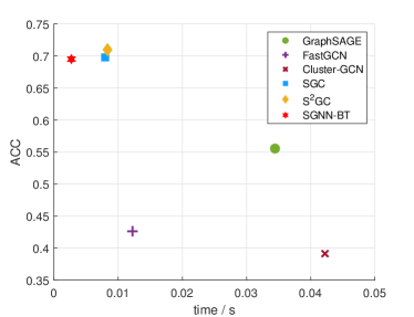
(a) Pubmed (clustering)

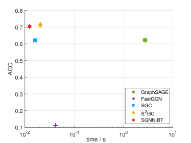
(b) Reddit (clustering)

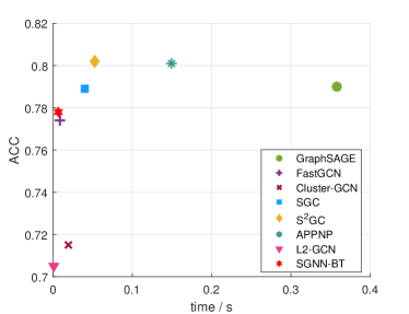
(c) Pubmed (classification)

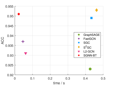
(d) Reddit (classification)

Figure 2: Performance and training efficiency of several scalable GNNs. The efficiency metric is computed by “Consuming Time / # Iterations”. The consuming time begins from loading data into RAM. The first line shows the result of node clustering and the second line is the result of node classification.

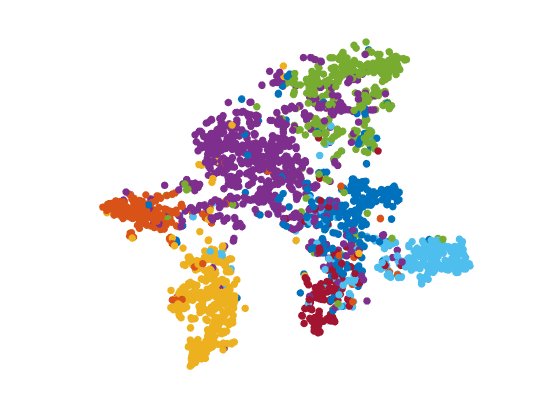
(a) GCN on Cora

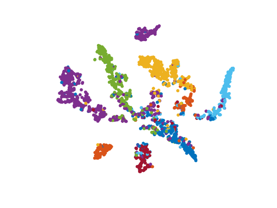
(b) SGNN on Cora

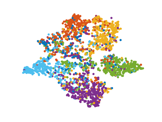
(c) GCN on Citeseer

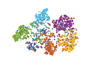
(d) SGNN on Citeseer

Figure 3: Visualization of SGNN comprised of 3 modules and 3-layer GCN on node classification. For SGNN, the output of $\mathcal{M}_{3}$ is visualized. For GCN, the output of the final GCN-layer is visualized.

5 Experiments

In this section, we conduct experiments to investigate whether the performance of SGNN could approach the performance of the original $L$-layer GNN in a highly-efficient way and what the impact of the non-linearity and flexibility brought by the decoupling is. To sufficiently answer the above 2 problems, both node clustering and semi-supervised node classification are used. Due to the limitation of space, only 4 common datasets, including Cora, Citeseer, Pubmed [47], and Reddit [14]. Cora and Citeseer contain thousands of nodes. Pubmed has nearly 20 thousands nodes and Reddit contains more than 200 thousands nodes, which are middle-scale and large-scale datasets respectively. The details of four common datasets are shown in Table 1. More experiments on OGB datasets can be found in Section 5.4.

Table 2: Node clustering results

Datasets	Cora		Citeseer		PubMed		Reddit
	ACC	NMI	ACC	NMI	ACC	NMI	ACC	NMI
K-Means	0.4922	0.3210	0.5401	0.3054	0.5952	0.2780	0.1927	0.2349
ARGA	0.6400	0.4490	0.5730	0.3500	0.6807	0.2757	N/A	N/A
MGAE	0.6806	0.4892	0.6691	0.4158	0.5932	0.2957	N/A	N/A
GraphSAGE	0.6163	0.4826	0.5664	0.3425	0.5554	0.0943	0.6225	0.7291
FastGAE	0.3527	0.1553	0.2672	0.1178	0.4262	0.0442	0.1115	0.0715
ClusterGAE	0.4579	0.2261	0.4182	0.1767	0.3913	0.0001	N/A	N/A
GAE	0.5960	0.4290	0.4080	0.1760	0.6861	0.2957	N/A	N/A
AGC (SGC)	0.6892	0.5368	0.6700	0.4113	0.6978	0.3159	0.5833	0.6894
SGNN-FT	0.6278	0.5075	0.6141	0.3776	0.6444	0.2312	0.5943	0.7156
SGNN-BT	0.7463	0.5546	0.6730	0.4159	0.6951	0.3337	0.7042	0.7601
S2GC	0.6960	0.5471	0.6911	0.4287	0.7098	0.3321	0.7011	0.7509
GAE-S2GC	0.6976	0.5317	0.6435	0.3969	0.6528	0.2452	0.6272	0.7158
SGNN-S2GC	0.7223	0.5404	0.6822	0.4243	0.7084	0.3302	0.7023	0.7575

5.1 Node Clustering

5.1.1 Experimental Settings

We first testify the effectiveness of SGNN on the node clustering. We compare our method against 10 methods, including a baseline clustering model K-means, three GCN models without considering training efficiency (GAE [9], ARGA [48], MGAE [37]), and six fast GCN models with GAE-loss (GraphSAGE [14], FastGAE [15], ClusterGAE [18], AGC [49] (an unsupervised extension of SGC [19]), S²GC [20], and GAE-S²GC).

The used codes are based on the publicly released implementation. To ensure fairness, all multi-layer GNN models consist of two layers and SGNN is comprised of two modules. For models that could be trained by stochastic algorithms, the size of mini-batch is set as 128. The learning rate is set as 0.001 and the number of epochs is set as 100. We set the size first layer as 128 and the second layer size as 64. In particular, when training every module of SGNN, 20% entries of the adjacency matrix are ignored. $\bm{U}$ is initialized as an identity matrix, and $\eta$ is set as $10^{3}$ by default. The number of backward training is set as 5 or 10. To investigate the effectiveness of backward training, we report the experimental results with sufficient training for each module, which is denoted by SGNN-FT, while SGNN with the proposed backward training is represented by SGNN-BT. To study the performance of SGNN with different base models, we choose a fully-separable GNN, S²GC, as the base model and this method is marked as SGNN-S²GC. As S²GC does not use the GAE framework, we also added a competitor, namely GAE-S²GC, which uses S²GC as the encoder, to ensure fairness. For SGNN-S²GC and GAE-S²GC, all extra hyper-parameters are simply set according to the original paper of S²GC for both node clustering and node classification. We do not tune the hyper-parameters of S²GC manually. All methods are run five times and the average scores are recorded. The result are summarized in Table 2.

Table 3: Test accuracy (%) of supervised SGNN averaged over 10 runs on 3 citation datasets

Datasets	Cora	Citeseer	Pubmed
GAT	83.0 $\pm$ 0.7	72.5 $\pm$ 0.7	79.0 $\pm$ 0.3
DGI	82.3 $\pm$ 0.6	71.8 $\pm$ 0.7	76.8 $\pm$ 0.6
GCNII	85.5 $\pm$ 0.5	73.4 $\pm$ 0.6	80.2 $\pm$ 0.4
FastGCN†	79.8 $\pm$ 0.3	68.8 $\pm$ 0.6	77.4 $\pm$ 0.3
GraphSAGE†	77.4 $\pm$ 0.6	66.7 $\pm$ 0.3	79.0 $\pm$ 0.3
Cluster-GCN†	65.3 $\pm$ 3.9	57.7 $\pm$ 2.3	71.5 $\pm$ 1.9
GCN	81.4 $\pm$ 0.4	70.9 $\pm$ 0.5	79.0 $\pm$ 0.4
SGC	81.0 $\pm$ 0.0	71.9 $\pm$ 0.1	78.9 $\pm$ 0.0
SGNN-BT	81.4 $\pm$ 0.5	70.2 $\pm$ 0.4	77.8 $\pm$ 0.3
S2GC	83.5 $\pm$ 0.0	73.6 $\pm$ 0.1	80.2 $\pm$ 0.0
SGNN-S2GC	83.8 $\pm$ 0.2	73.2 $\pm$ 0.3	80.2 $\pm$ 0.4

Table 4: Test accuracy (%) averaged over 5 runs on Reddit

Methods	Reddit
GAT	N/A
DGI	94.0
SAGE-mean	95.0
SAGE-GCN	93.0
FastGCN	93.7
Cluster-GCN	96.6
GCN	N/A
SGC	94.9
SGNN-BT	95.10 $\pm$ 0.02
S2GC	95.3
SGNN-S2GC	95.28 $\pm$ 0.03

5.1.2 Performance

From Table 2, we find that SGNN outperforms in most datasets. If the released codes could not run on Reddit due to out-of-memory (OOM), we put the notation “N/A” instead of results. In particular, SGNN-BT obtains good improvements on Reddit with high efficiency. Specifically speaking, it is about 8% higher than the well-known GraphSAGE. SGNN-FT performs above the average on some datasets. It usually outperforms GraphSAGE but fails to exceed SGC. Due to the deeper structure caused by multiple modules, the performance of SGNN excels the simple GAE. It also outperforms SGC due to more non-linearity brought by multiple modules. Note that S²GC and SGC are strong competitors, while SGNN can easily employ them as a base module since they are separable. From the ablation experiments, SGNN-BT works better than SGNN-FT, which indicates the necessity of the backward training.

We also investigate how the number of modules $L$ affects the node clustering accuracy and the results averaged over 5 runs are reported in Table 5. To ensure fairness, we also show the performance of GAE with the same depth though deeper GCN and GAE usually return unsatisfied results. Note that the neurons of each layers are set as $[256,128,64,32,16,16,16]$, respectively. It is not hard to find that SGNN is robust to the depth compared with the conventional GNNs.

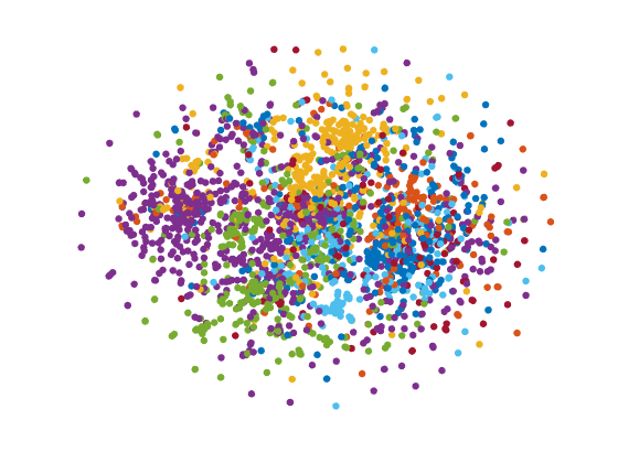
(a) $\bm{H}_{0}$: Input of $\mathcal{M}_{1}$

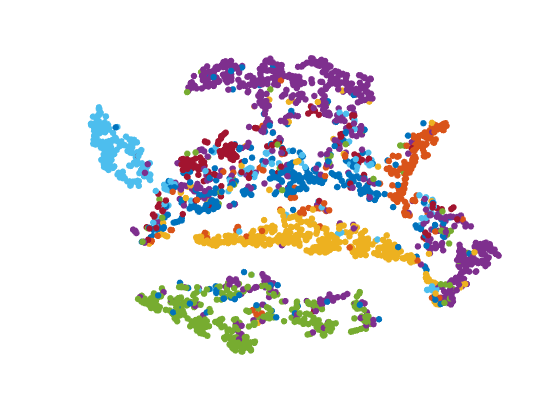
(b) $\bm{H}_{1}$: From $\mathcal{M}_{1}$ to $\mathcal{M}_{2}$

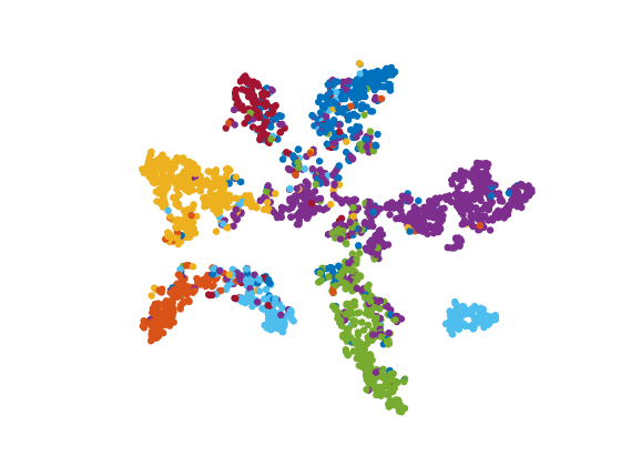
(c) $\bm{H}_{2}$: From $\mathcal{M}_{2}$ to $\mathcal{M}_{3}$

(d) $\bm{H}_{3}$: Output of $\mathcal{M}_{3}$

(e) $\bm{H}_{0}$: Input of $\mathcal{M}_{1}$

(f) $\bm{H}_{1}$: From $\mathcal{M}_{1}$ to $\mathcal{M}_{2}$

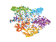
(g) $\bm{H}_{2}$: From $\mathcal{M}_{2}$ to $\mathcal{M}_{3}$

(h) $\bm{H}_{3}$: Output of $\mathcal{M}_{3}$

Figure 4: Visualization of a trained SGNN comprised of 3 modules on node classification of Cora and Citeseer. The first line shows the visualization of Cora and the bottom line shows the visualization of Citeseer.

(a) $\bm{H}_{0}$: Input of $\mathcal{M}_{1}$

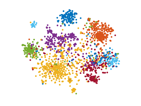
(b) $\bm{H}_{1}$: From $\mathcal{M}_{1}$ to $\mathcal{M}_{2}$

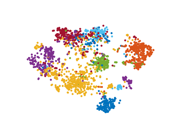
(c) $\bm{H}_{2}$: From $\mathcal{M}_{2}$ to $\mathcal{M}_{3}$

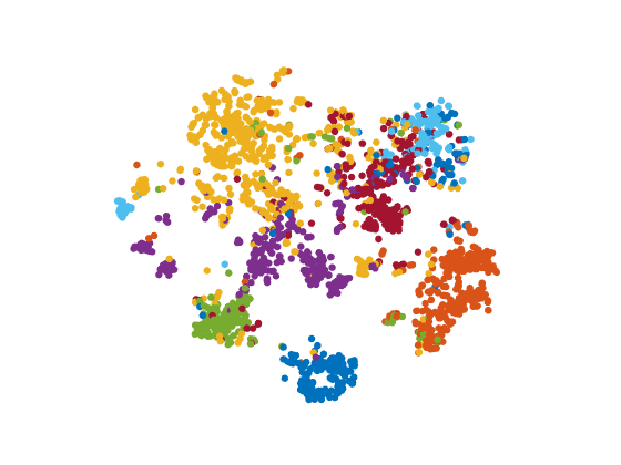
(d) $\bm{H}_{3}$: Output of $\mathcal{M}_{3}$

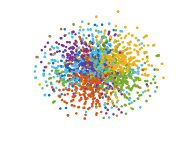
(e) $\bm{H}_{0}$: Input of $\mathcal{M}_{1}$

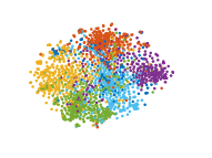
(f) $\bm{H}_{1}$: From $\mathcal{M}_{1}$ to $\mathcal{M}_{2}$

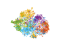
(g) $\bm{H}_{2}$: From $\mathcal{M}_{2}$ to $\mathcal{M}_{3}$

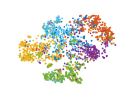
(h) $\bm{H}_{3}$: Output of $\mathcal{M}_{3}$

Figure 5: Visualization of a trained SGNN comprised of 3 modules on node clustering of Cora and Citeseer. The first line is visualization on Cora and the second line is visualization on Citeseer.

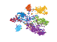
(a) $\bm{H}_{1}$ after 1 epoch

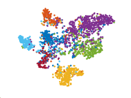
(b) $\bm{H}_{1}$ after 2 epochs

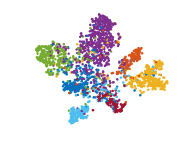
(c) $\bm{H}_{1}$ after 3 epochs

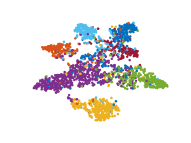
(d) $\bm{H}_{1}$ after 5 epochs

Figure 6: t-SNE Visualization of the output of $\mathcal{M}_{1}$ from a trained SGNN comprised of 3 modules on node classification of Citeseer.

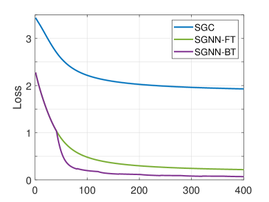
(a) Cora

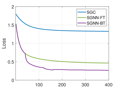
(b) Pubmed

Figure 7: Convergence curve of the final loss. The order of SGC is set as $L$. The backward training significantly decreases the final loss and the non-linearity also plays an important role.

5.1.3 Efficiency

Figure 2 shows the consuming time of several GNNs with higher efficiency on Pubmed and Reddit. Instead of neglecting the preprocessing operation, we measure the efficiency through a more rational way. We record the totally consuming time after loading data into RAM and then divide the total number of updating parameters of GNNs. The measurement could reflect the real difference of diverse training techniques aiming to apply batch-based algorithms to GNN. It should be emphasized the reason why SGC is worse than SGNN regarding the consuming time. The key point is the different costs of their preprocessing operation. For an $L$-order SGC, the computation cost of $\bm{P}^{L}\bm{X}$ is at least $\mathcal{O}(\|\bm{A}\|_{0}Ld)$ while SGNN with $L$ first-order modules totally requires $\mathcal{O}(\|\bm{A}\|_{0}\sum_{i=1}^{L}d_{i})$ for the same preprocessing operation. The metric also provides a fair comparison between SGC and other models since the stopping criteria are always different.

Table 5: Investigation about the impact of $L$ on SGNN and GAE regarding node clustering.

$L$	Cora			Citeseer			Pubmed
	SGNN	GAE	FastGAE	SGNN	GAE	FastGAE	SGNN	GAE	FastGAE
2	0.75	0.60	0.35	0.67	0.41	0.27	0.70	0.69	0.43
3	0.66	0.63	0.33	0.65	0.58	0.25	0.64	0.64	0.42
4	0.68	0.65	0.33	0.59	0.58	0.24	0.64	0.60	0.41
5	0.69	0.62	0.33	0.53	0.45	0.24	0.64	0.60	0.41
6	0.69	0.53	0.32	0.44	0.32	0.24	0.64	0.48	0.41
7	0.68	0.52	0.32	0.44	0.31	0.24	0.64	0.46	N/A

5.2 Node Classification

5.2.1 Experimental Setting

We also conduct experiments of semi-supervised classification on four datasets. The split of datasets follows [19] which is shown in Table 1. We compare SGNN against GCN [4], GAT [6], DGI [50], APPNP [51], L2-GCN [34] FastGCN [15], GraphSAGE [14], Cluster-GCN [18], SGC [19], GCNII [52], and S²GC [20]. Similarly, we testify SGNN with two different base models, namely SGNN-BT and SGNN-S²GC. For GraphSAGE, we use the mean operator by default and some notations are added if the extra operators are used. On citation networks, the learning rate is set as $0.01$, while it is $10^{-4}$ on Reddit. Since the nodes for training are less than 200 on citation networks, we use all training points in each iteration for all methods while we sample 256 points as a mini-batch for approaching expected features during backward training of SGNN. On Reddit, the batch size of all batch-based models is set as 512. We do not apply the early stopping criterion used in [4] and the max iteration follows the setting of SGC. The embedding dimensions of each module are the same as the setting in node clustering. For the sake of fairness, we report the results obtained by SGNN with two modules using first-order operation. The forward training loss is defined in Eq. (4). Moreover, all compared models share an identical implementation of their mini-batch iterators, loss function and neighborhood sampler (when applicable). The balance coefficient of $\mathcal{L}_{FT}$ and $\mathcal{L}_{BT}$ is set as $1$ by default. We report the results averaged over 10 runs on citation datasets and 5 runs on Reddit in Table 4 and Table 4. The hyper-parameters are shared for different datasets which are optimized on Cora.

Table 6: Node Classification Results on Large Datasets

Datasets	Products		Arxiv
	Test Acc	Val Acc	Test Acc	Val Acc
MLP	61.06	75.54	55.50	57.65
GCN	75.64	92.00	71.74	73.00
GraphSAGE	78.50	92.24	71.49	72.77
Cluster-GCN	78.97	92.12	N/A	N/A
Softmax	47.70	N/A	52.77	N/A
SGC	68.87	N/A	68.78	N/A
S2GC	70.22	N/A	70.15	N/A
SGNN-BT	74.44	91.13	71.57	71.66

5.2.2 Performance

The results of compared methods in Table 4 are taken from the corresponding papers. When the experimental results are missed, we run the publicly released codes and the corresponding records are superscripted by ${\dagger}$. From Tables 4 and 4, we conclude that SGNN outperforms the models with neighbor sampling such as GraphSAGE, FastGCN, and ClusterGCN on citation networks and the performance of SGNN exceeds most models on Reddit. On simple citation networks, SGNN loses the least accuracy compared with other batch-based models, which is close to GCN. Owing to the separability of each module, the batch sampling requires no neighbor sampling and causes no loss of graph information. Note that we simply employ the single-layer GCN as the base modules in our experiments, while some high-order methods that obtain competitive results are also available for SGNN. Although some methods achieve preferable results, they either fail to run or obtain unsatisfactory results on large-scale datasets. Besides, we also show the comparison of efficiency on node classification task in Table 2.

5.2.3 Visualization to Show Impact of the Decoupling

In Figure 3, we visualize the output of a 3-module SGNN and a 3-layer GCN to directly show that the decoupling would not cause the trivial features, which corresponds to the theoretical conclusion in Section 4. To show the benefit of the non-linearity brought by SGNN and the backward training, the convergence curves of SGC, SGNN-FT, and SGNN-BT are shown in Figure 7. Note that the figure shows the variation of the final loss. In SGNN, the final loss is the loss of $\mathcal{M}_{L}$, while it is the unique training loss in SGC. SGC with $L$-order graph operation is used. From this figure, we can conclude that: (1) The non-linearity does lead to a better loss value; (2) The backward training significantly decreases the loss. In summary, the decoupling empirically does not cause the negative impact.

5.3 Visualization

We also provide more visualizations in Figures 4 and 5. We run SGNN with 3 GNN modules and visualize the input and output of $\mathcal{M}_{1}$, $\mathcal{M}_{2}$, and $\mathcal{M}_{3}$ through $t$-SNE on Cora and Citeseer, for node clustering and node classification. The purpose of these two figures is to empirically investigate whether the decoupling would cause the accumulation of residuals and errors. The experimental results support the theoretical results that are provided in Section 4. One may concern the impact of $\eta$ (trade-off coefficient between $\mathcal{L}_{FT}$ and $\mathcal{L}_{B}T$) on the performance. We testify SGNN with different $\eta$ from $\{10^{-5},10^{-3},10^{-1},10^{1},10^{3},10^{5}\}$ and find that $\eta=10^{3}$ usually leads to good results. Accordingly, we only report results SGNN with $\eta=10^{3}$ in this paper. Moreover, we show the impact of $\eta$ to node clustering on Cora and Citeseer in Figure 8.

Moreover, we show the output of $\mathcal{M}_{1}$ of different periods in Figure 6, in order to show the impact of the backward training. From the figure, we find that BT indeed affects the latent features, which is particularly apparent in Figure 6(d).

5.4 Experiments on OGB Datasets

We further show some experiments of node classification on two OGB datasets, OGB-Products and OGB-Arxiv, which are downloaded from https://ogb.stanford.edu/docs/nodeprop/. The OGB-Products contains more than 2 million nodes and OGB-Arxiv contains more than 150 thousand nodes.

It should be emphasized that we only use the simple single-layer GCN as the base module of SGNN. The performance can be further improved by incorporating different models such as GCNII, GIN, etc. In particular, we only tune hyper-parameters on Arxiv, and we simply report results of SGNN with settings from Reddit.

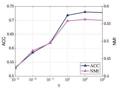
(a) Cora

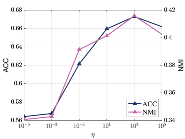
(b) Citeseer

Figure 8: Impact of $\eta$ to node clustering on Cora and Citeseer

6 Conclusion and Future Works

In this paper, we propose the Stacked Graph Neural Networks (SGNN). We first decouple a multi-layer GNN into multiple simple GNNs, which is formally defined as separable GNNs in our paper to ensure the availability of batch-based optimization without loss of graph information. The bottleneck of the existing stacked models is that the information delivery is only unidirectional, and therefore a backward training mechanism is developed to make the former modules perceive the latter ones. We also theoretically prove that the residual of linear SGNN would not accumulate in most cases for unsupervised graph tasks. The theoretical and experimental results show that the proposed framework is more than an efficient method and it may deserve further investigation in the future. The theoretical analysis focuses on linear SGNN and the generalization bound is also not investigated in this paper. Therefore, they will be the core of our future work. Moreover, as $\mathcal{L}_{FT}$ could be any losses, how to choose the most appropriate loss for each module will be also a crucial topic in our future works.

Appendix A Proofs

Appendix B Lemma for Proofs

Lemma B.1.

For two given symmetric matrices $\bm{A}$ and $\bm{B}$, $\bm{A}$ and $\bm{B}$ share the same eigenspace if and only if $\bm{A}$ and $\bm{B}$ commute.

Proof.

First, if $\bm{A}$ and $\bm{B}$ share the same eigenspace, then there exists $\bm{P}$ such that

$$\bm{A}=\bm{P}\bm{\Lambda}_{A}\bm{P}^{T},\bm{B}=\bm{P}\bm{\Lambda}_{B}\bm{P}^{T}.$$ (8)

Accordingly, we have $\bm{A}\bm{B}=\bm{P}\bm{\Lambda}_{A}\bm{\Lambda}_{B}\bm{P}^{T}=\bm{BA}$.

Then, we turn to prove the converse. If $\bm{A}$ and $\bm{B}$ commute, suppose that $\bm{A}\bm{u}=\lambda\bm{u}$ and then

$$\bm{ABu}=\bm{BAu}=\lambda\bm{Bu}.$$ (9)

Apply eigenvalue decomposition, we have $\bm{A}=\bm{U}\bm{\Lambda}\bm{U}^{T}$. Note that if $\bm{A}\bm{u}_{1}=\lambda_{1}\bm{u}_{1}$, $\bm{A}\bm{u}_{2}=\lambda_{2}\bm{u}_{2}$, and $\lambda_{1}\neq\lambda_{2}$, then $\bm{u}_{2}^{T}\bm{B}\bm{u}_{1}=0$ since $\bm{B}\bm{u}_{1}$ is also an eigenvector associated with $\lambda_{1}$. Therefore, $\bm{U}^{T}\bm{BU}$ is a block-diagonal matrix, i.e.,

$$\bm{U}^{T}\bm{B}\bm{U}=\left[\begin{array}[]{c c c c}\bm{C}_{1}&&&\\ &\bm{C}_{2}&&\\ &&\ddots&\\ &&&\bm{C}_{k}\\ \end{array}\right].$$ (10)

Apply eigendecomposition to $\bm{C}_{i}$,

$$\bm{C}_{i}=\bm{U}_{i}\bm{\Lambda}_{i}\bm{U}_{i}^{T}.$$ (11)

Denote

$$\bm{T}=\left[\begin{array}[]{c c c c}\bm{U}_{1}&&&\\ &\bm{U}_{2}&&\\ &&\ddots&\\ &&&\bm{U}_{k}\\ \end{array},\right]$$ (12)

and $\bm{V}=\bm{U}\bm{T}$, which leads to

$$\bm{T}^{T}\bm{U}^{T}\bm{B}\bm{U}\bm{T}=\bm{\Lambda}_{B}~{}~{}\textrm{and}~{}~{}\bm{T}^{T}\bm{U}^{T}\bm{A}\bm{U}\bm{T}=\bm{\Lambda}_{A}$$ (13)

where $\bm{V}^{T}\bm{V}=\bm{I}$. Hence, the lemma is proved. ∎

Appendix C Proof of Theorem 4.1

Theorem.

Let $\delta=1-\cos(\theta_{*}/2)$ and $\theta_{*}=\theta((\bm{P}-\bm{X}\bm{X}^{T})\bm{Q},\bm{Q}(\bm{P}-\bm{X}\bm{X}^{T}))$ where $\bm{Q}=\bm{U}_{o}\bm{U}_{o}^{T}-\bm{I}/2$ and $o=\min({\rm rank}(\bm{X}),k)$. Under Assumption 4.1, if $\|\bm{P}-\bm{H}\bm{H}^{T}\|=\varepsilon\leq\mathcal{O}(\delta)$ and $\sigma_{*}\leq\mathcal{O}(\sqrt{\delta})$ where $\sigma_{*}$ is the $(o+1)$-th largest singular value of $\bm{X}$, then there exists $\bm{W}\in\mathbb{R}^{d\times k}$ so that $\|\bm{P}-\bm{H}\bm{H}^{T}\|\leq\varepsilon$ In other words, if $\varepsilon$ is small enough, then $\bm{H}\bm{H}^{T}$ could be a better approximation than $\bm{X}\bm{X}^{T}$.

Proof.

Use the notation $\ell(\cdot,\cdot,\cdot)$ as the reconstruction loss

$$\ell(\bm{P},\bm{X},\bm{W})=\|\bm{P}-\bm{PXW}\bm{W}^{T}\bm{X}^{T}\bm{P}^{T}\|.$$ (14)

According to the conditions, we define

$$\bm{E}=\bm{P}-\bm{X}\bm{X}^{T}\Rightarrow\|\bm{E}\|=\varepsilon.$$ (15)

Apply SVD, we can factorize $\bm{X}$ as

$$\bm{X}=\bm{U}_{o}\bm{\Sigma}_{o}\bm{V}_{o}^{T}+\bm{U}_{e}\bm{\Sigma}_{e}\bm{V}_{e}^{T},$$ (16)

where $e=d-o$. Clearly, we have $\bm{V}_{o}^{T}\bm{V}_{e}=\bm{0}$ and thus

$$\begin{split}\bm{P}=\bm{X}\bm{X}^{T}+\bm{E}=\bm{U}_{k}\bm{\Sigma}_{k}^{2}\bm{U}_{k}^{T}+\bm{U}_{e}\bm{\Sigma}_{e}^{2}\bm{U}_{e}^{T}+\bm{E}.\end{split}$$ (17)

Therefore, $\bm{H}\bm{H}^{T}$ can be written as

$$\bm{H}\bm{H}^{T}=\bm{P}(\bm{U}_{o}\bm{\Sigma}_{o}\bm{V}_{o}^{T}+\bm{U}_{e}\bm{\Sigma}_{e}\bm{V}_{e}^{T})\bm{W}\bm{W}^{T}(\bm{V}_{o}\bm{\Sigma}_{o}\bm{U}_{o}^{T}+\bm{V}_{e}\bm{\Sigma}_{e}\bm{U}_{e}^{T})\bm{P}.$$ (18)

Let $\bm{W}_{0}$ be a valid solution as

$$\bm{W}_{0}=\begin{cases}\bm{W}_{0}~{}~{}&s.t.~{}\bm{V}_{k}^{T}\bm{W}_{0}=\bm{\Sigma}_{k}^{-2}~{}~{}~{}~{}{\rm if~{}rank}(\bm{X})=k\\ [\bm{W}_{r};\bm{0}]~{}~{}&s.t.~{}\bm{V}_{r}^{T}\bm{W}_{r}=\bm{\Sigma}_{r}^{-2}~{}~{}~{}~{}{\rm if~{}rank}(\bm{X})=r\leq k\end{cases}.$$ (19)

By the above definition, $\bm{V}_{e}^{T}\bm{W}=\bm{0}$. Therefore, with ${\rm rank}(\bm{X})>k$,

$$\begin{split}&\|\bm{H}\bm{H}^{T}-\bm{P}\|\\ =&\|\bm{U}_{k}\bm{\Sigma}_{k}^{3}\bm{V}_{k}\bm{W}_{0}\bm{W}_{0}^{T}\bm{V}_{k}\bm{\Sigma}_{k}^{3}\bm{U}_{k}^{T}+\bm{E}\bm{U}_{k}\bm{\Sigma}_{k}\bm{V}_{k}\bm{W}_{0}\bm{W}_{0}^{T}\bm{V}_{k}\bm{\Sigma}_{k}^{3}\bm{U}_{k}^{T}\\ &~{}+\bm{U}_{k}\bm{\Sigma}_{k}^{3}\bm{V}_{k}\bm{W}_{0}\bm{W}_{0}^{T}\bm{V}_{k}\bm{\Sigma}_{k}\bm{U}_{k}^{T}\bm{E}+\bm{E}\bm{U}_{k}\bm{\Sigma}_{k}\bm{V}_{k}\bm{W}_{0}\bm{W}_{0}^{T}\bm{V}_{k}\bm{\Sigma}_{k}\bm{U}_{k}^{T}\bm{E}-\bm{P}\|\\ =&\|\bm{U}_{k}\bm{\Sigma}_{k}^{2}\bm{U}_{k}^{T}+\bm{E}\bm{U}_{k}\bm{U}_{k}^{T}+\bm{U}_{k}\bm{U}_{k}^{T}\bm{E}+\bm{E}\bm{U}_{k}\bm{\Sigma}_{k}^{-2}\bm{U}_{k}^{T}\bm{E}-\bm{U}_{k}\bm{\Sigma}_{k}^{2}\bm{U}_{k}^{T}-\bm{U}_{e}\bm{\Sigma}_{e}^{2}\bm{U}_{e}^{T}-\bm{E}\|\\ =&\|\bm{E}\bm{U}_{k}\bm{U}_{k}^{T}+\bm{U}_{k}\bm{U}_{k}^{T}\bm{E}+\bm{E}\bm{U}_{k}\bm{\Sigma}_{k}^{-2}\bm{U}_{k}^{T}\bm{E}-\bm{U}_{e}\bm{\Sigma}_{e}^{2}\bm{U}_{e}^{T}-\bm{E}\|\\ \leq&\|\bm{E}\bm{U}_{k}\bm{U}_{k}^{T}+\bm{U}_{k}\bm{U}_{k}^{T}\bm{E}-\bm{E}\|+\|\bm{E}\bm{U}_{k}\bm{\Sigma}_{k}^{-2}\bm{U}_{k}^{T}\bm{E}\|+\|\bm{U}_{e}\bm{\Sigma}_{e}^{2}\bm{U}_{e}^{T}\|.\\ \end{split}$$ (20)

Similarly, if ${\rm rank}(\bm{X})=r\leq k$,

$$\|\bm{H}\bm{H}^{T}-\bm{P}\|= \|\bm{E}\bm{U}_{r}\bm{U}_{r}^{T}+\bm{U}_{r}\bm{U}_{r}^{T}\bm{E}+\bm{E}\bm{U}_{r}\bm{\Sigma}_{r}^{-2}\bm{U}_{r}^{T}\bm{E}-\bm{E}\|$$ (21)

$$\leq \|\bm{E}\bm{U}_{r}\bm{U}_{r}^{T}+\bm{U}_{r}\bm{U}_{r}^{T}\bm{E}-\bm{E}\|+\|\bm{E}\bm{U}_{r}\bm{\Sigma}_{r}^{-2}\bm{U}_{r}^{T}\bm{E}\|.$$ (22)

Now we focus on the general case, ${\rm rank}(\bm{X})>k$ and the conclusion can be easily extended into the low-rank case. Note that

$$\|\bm{E}(\bm{U}_{k}\bm{U}_{k}^{T}-\frac{1}{2}\bm{I})\|=\|(\bm{U}_{k}\bm{U}_{k}^{T}-\frac{1}{2}\bm{I})\bm{E}\|,$$ (23)

and the first term can be written as

$$\|\bm{E}\bm{U}_{k}\bm{U}_{k}^{T}+\bm{U}_{k}\bm{U}_{k}^{T}\bm{E}-\bm{E}\|^{2}$$

$$= \|\bm{E}(\bm{U}_{k}\bm{U}_{k}^{T}-\frac{1}{2}\bm{I})+(\bm{U}_{k}\bm{U}_{k}^{T}-\frac{1}{2}\bm{I})\bm{E}\|^{2}$$

$$= \|\bm{E}(\bm{U}_{k}\bm{U}_{k}^{T}-\frac{1}{2}\bm{I})\|^{2}+\|(\bm{U}_{k}\bm{U}_{k}^{T}-\frac{1}{2}\bm{I})\bm{E}\|^{2}+2\langle\bm{E}(\bm{U}_{k}\bm{U}_{k}^{T}-\frac{1}{2}\bm{I}),(\bm{U}_{k}\bm{U}_{k}^{T}-\frac{1}{2}\bm{I})\bm{E}\rangle$$

$$= 2\|\bm{E}(\bm{U}_{k}\bm{U}_{k}^{T}-\frac{1}{2}\bm{I})\|^{2}+2s\|\bm{E}(\bm{U}_{k}\bm{U}_{k}^{T}-\frac{1}{2}\bm{I})\|^{2}$$

$$= 2(1+s)\|\bm{E}(\bm{U}_{k}\bm{U}_{k}^{T}-\frac{1}{2}\bm{I})\|^{2},$$

where

$$s=\frac{\langle\bm{E}(\bm{U}_{k}\bm{U}_{k}^{T}-\frac{1}{2}\bm{I}),(\bm{U}_{k}\bm{U}_{k}^{T}-\frac{1}{2}\bm{I})\bm{E}\rangle}{\|\bm{E}(\bm{U}_{k}\bm{U}_{k}^{T}-\frac{1}{2}\bm{I})\|^{2}}.$$ (24)

Due to that

$$\|\bm{E}(\bm{U}_{k}\bm{U}_{k}^{T}-\frac{1}{2}\bm{I})\|^{2} ={\rm tr}(\bm{E}^{2}(\bm{U}_{k}\bm{U}_{k}^{T}-\frac{1}{2}\bm{I}))$$

$$={\rm tr}(\bm{E}^{2}(\bm{U}_{k}\bm{U}_{k}^{T}\bm{U}_{k}\bm{U}_{k}^{T}-2\times\frac{1}{2}\bm{U}_{k}\bm{U}_{k}^{T}+\frac{1}{4}\bm{I}))$$

$$=\frac{1}{4}{\rm tr}(\bm{E}^{2})=\frac{1}{4}\varepsilon^{2},$$

we have

$$\|\bm{E}\bm{U}_{k}\bm{U}_{k}^{T}+\bm{U}_{k}\bm{U}_{k}^{T}\bm{E}-\bm{E}\| =\sqrt{2(1+s)}\|\bm{E}(\bm{U}_{k}\bm{U}_{k}^{T}-\frac{1}{2}\bm{I})\|=\sqrt{\frac{1+s}{2}}\varepsilon.$$ (25)

Let $\bm{Q}=(\bm{U}_{k}\bm{U}_{k}^{T}-\bm{I}/2)$ and $s$ can be reformulated as

$$s=\cos(\bm{E}\bm{Q},\bm{Q}\bm{E}),$$ (26)

and we have the following definition

$$\theta_{*}=\arccos(s)=\theta(\bm{E}\bm{Q},\bm{Q}\bm{E}).$$ (27)

According to Lemma B.1, Assumption 4.1 indicates that

$$\bm{E}(\bm{U}_{k}\bm{U}_{k}^{T}-\frac{1}{2}\bm{I})=(\bm{U}_{k}\bm{U}_{k}^{T}-\frac{1}{2}\bm{I})\bm{E}\Rightarrow s<1.$$ (28)

And therefore, $\sqrt{(1+s)/2}\in[0,1)$. Let $\delta=1-\sqrt{(1+s)/2}=1-\cos(\theta_{*}/2)>0$ and the above equation can be reformulated as

$$\|\bm{E}\bm{U}_{k}\bm{U}_{k}^{T}+\bm{U}_{k}\bm{U}_{k}^{T}\bm{E}-\bm{E}\|=(1-\delta)\varepsilon.$$ (29)

The second term can be formulated as

$$\|\bm{E}\bm{U}_{k}\bm{\Sigma}_{k}^{-2}\bm{U}_{k}^{T}\bm{E}\|\leq \|\bm{U}_{k}\bm{\Sigma}_{k}^{-2}\bm{U}_{k}^{T}\|\varepsilon^{2}$$ (30)

$$= \varepsilon^{2}\sqrt{{\rm tr}(\bm{U}_{k}\bm{\Sigma}_{k}^{-4}\bm{U}_{k}^{T})}=\varepsilon^{2}\sqrt{{\rm tr}(\bm{\Sigma}^{-4}\bm{U}_{k}^{T}\bm{U}_{k})}$$ (31)

$$= \varepsilon^{2}\sqrt{\sum_{i=1}^{k}\frac{1}{\sigma_{i}^{4}}}\leq\sqrt{r}\frac{\varepsilon^{2}}{\sigma_{k}^{2}},$$ (32)

while the third term is

$$\|\bm{U}_{e}\bm{\Sigma}_{e}^{2}\bm{U}_{e}^{T}\|=\|\bm{\Sigma}_{e}^{2}\|=(\sum_{i=k+1}^{n}\sigma_{i}^{4})^{1/2}\leq\sqrt{n-k}\sigma_{*}^{2},$$ (33)

To sum up, the error of $\mathcal{M}$ is bounded as

$$\|\bm{H}\bm{H}^{T}-\bm{P}\|\leq(1-\delta)\varepsilon+\sqrt{k}\frac{\varepsilon^{2}}{\sigma_{k}^{2}}+\sqrt{e}\sigma_{*}^{2}.$$ (34)

If

$$\sqrt{k}\frac{\varepsilon}{\sigma_{k}^{2}}\leq\frac{\delta}{2}\Rightarrow\varepsilon\leq\frac{\delta\sigma_{k}^{2}}{2\sqrt{k}},$$ (35)

and

$$\sqrt{n-k}\sigma_{*}^{2}\leq\frac{\delta}{2}\Rightarrow\sigma_{*}\leq\sqrt{\frac{\delta}{2\sqrt{n-k}}}.$$ (36)

then $\|\bm{H}\bm{H}^{T}-\bm{P}\|\leq\varepsilon$. In other words, when $\varepsilon\leq\mathcal{O}(\delta)$ and $\sigma_{*}\leq\mathcal{O}(\sqrt{\delta})$, the error will be bounded by $\varepsilon$.

For the case that ${\rm rank}(\bm{X})=r<k$, it is not hard to verify that

$$\|\bm{H}\bm{H}^{T}-\bm{P}\| \leq\|\bm{E}\bm{U}_{r}\bm{U}_{r}^{T}+\bm{U}_{r}\bm{U}_{r}^{T}\bm{E}-\bm{E}\|+\|\bm{E}\bm{U}_{r}\bm{\Sigma}_{r}^{-2}\bm{U}_{r}^{T}\bm{E}\|$$ (37)

$$\leq(1-\delta)\varepsilon+\sqrt{r}\frac{\varepsilon^{2}}{\sigma_{r}^{2}}.$$ (38)

As

$$\sqrt{r}\frac{\varepsilon}{\sigma_{r}^{2}}\leq\frac{\delta}{2}\Rightarrow\varepsilon\leq\frac{\delta\sigma_{r}^{2}}{2\sqrt{r}}=\mathcal{O}(\delta),$$ (39)

and $\sigma_{*}=0\leq\mathcal{O}(\sqrt{\delta})$, we get $\|\bm{H}\bm{H}^{T}-\bm{P}\|\leq\varepsilon$. Hence, we have

$$\min_{\bm{W}}\ell(\bm{P},\bm{X},\bm{W})\leq\ell(\bm{P},\bm{X},\bm{W}_{0})\leq\varepsilon,$$ (40)

and the theorem is proved. ∎

Appendix D Proof of Theorem 4.2

Theorem.

If Assumption 4.1 does not hold, then there exists $\bm{W}\in\mathbb{R}^{d\times k}$ so that $\|\bm{P}-\bm{H}\bm{H}\|\leq\varepsilon+\mathcal{O}(\sigma_{*}^{2})$.

Proof.

According to Ineq. (20),

$$\|\bm{H}\bm{H}^{T}-\bm{P}\|\leq\|\bm{E}\bm{U}_{k}\bm{U}_{k}^{T}+\bm{U}_{k}\bm{U}_{k}^{T}\bm{E}-\bm{E}\|+\|\bm{E}\bm{U}_{k}\bm{\Sigma}_{k}^{-2}\bm{U}_{k}^{T}\bm{E}\|+\|\bm{U}_{e}\bm{\Sigma}_{e}^{2}\bm{U}_{e}^{T}\|.$$ (41)

Suppose that $\bm{E}=\bm{U}\bm{\Lambda}\bm{U}^{T}$ so that $\bm{P}=\bm{U}(\bm{S}+\bm{\Lambda})\bm{U}^{T}$ where $\bm{S}=\bm{\Sigma}\bm{\Sigma}^{T}={\rm diag}(\bm{\Sigma}_{k}^{2};\bm{0})$.

$$\bm{P}=\bm{U}(\bm{S}+\bm{\Lambda})\bm{U}^{T} =[\bm{U}_{r},\bm{U}_{e}]\left[\begin{array}[]{c c}\bm{\Sigma}_{r}^{2}+\bm{\Lambda}_{r}&\bm{0}\\ \bm{0}&\bm{\Sigma}_{e}^{2}+\bm{\Lambda}_{e}\end{array}\right]\left[\begin{array}[]{c}\bm{U}_{r}^{T}\\ \bm{U}_{e}^{T}\end{array}\right]$$

$$=\bm{U}_{k}(\bm{\Sigma}_{k}^{2}+\bm{\Lambda}_{k})\bm{U}_{k}^{T}+\bm{U}_{e}(\bm{\Sigma}_{e}^{2}+\bm{\Lambda}_{e})\bm{U}_{e}^{T}$$

Then let $\bm{V}_{k}\bm{W}=(\bm{\Sigma}_{k}^{3}+\bm{\Lambda}_{k}\bm{\Sigma}_{k})^{\dagger}(\bm{\Sigma}_{k}^{2}+\bm{\Lambda}_{k})^{1/2}$

$$\begin{split}\|\bm{P}-\bm{H}\bm{H}^{T}\|&=\|\bm{U}(\bm{S}+\bm{\Lambda})\bm{\Sigma}\bm{V}^{T}\bm{W}\bm{W}^{T}\bm{V}\bm{\Sigma}^{T}(\bm{S}+\bm{\Lambda})\bm{U}^{T}-\bm{P}\|\\ &=\|\bm{U}_{k}(\bm{\Sigma}_{k}^{3}+\bm{\Lambda}_{k}\bm{\Sigma}_{k})\bm{V}_{k}^{T}\bm{W}\bm{W}^{T}\bm{V}_{k}(\bm{\Sigma}_{k}^{3}+\bm{\Lambda}_{k}\bm{\Sigma}_{k})\bm{U}_{k}^{T}-\bm{P}\|\\ &=\|\bm{U}_{k}\hat{\bm{I}}(\bm{\Sigma}_{k}^{2}+\bm{\Lambda}_{k})\hat{\bm{I}}\bm{U}_{k}^{T}-\bm{U}_{k}(\bm{\Sigma}_{k}^{2}+\bm{\Lambda}_{k})\bm{U}_{k}^{T}-\bm{U}_{e}(\bm{\Sigma}_{e}^{2}+\bm{\Lambda}_{e})\bm{U}_{e}^{T}\|\\ &=\|\bm{U}_{e}(\bm{\Sigma}_{e}^{2}+\bm{\Lambda}_{e})\bm{U}_{e}^{T}\|\leq\|\bm{\Sigma}_{e}^{2}\|+\|\bm{\Lambda}_{e}\|\\ &\leq\varepsilon+\mathcal{O}(\sigma_{*}^{2})\end{split}$$ (42)

where $\hat{\bm{I}}=(\bm{\Sigma}_{k}^{3}+\bm{\Lambda}_{k}\bm{\Sigma}_{k})(\bm{\Sigma}_{k}^{3}+\bm{\Lambda}_{k}\bm{\Sigma}_{k})^{{\dagger}}=\bm{\Sigma}_{k}(\bm{\Sigma}_{k}^{2}+\bm{\Lambda}_{k})(\bm{\Sigma}_{k}^{2}+\bm{\Lambda}_{k})^{\dagger}\bm{\Sigma}_{k}^{-1}$. Clearly, $\hat{\bm{I}}=\mathbbm{1}\{\bm{\Sigma}_{r}^{2}+\bm{\Lambda}_{r}\neq 0\}$. Therefore, Hence, the theorem is proved. ∎

Corollary D.1.

If Assumption 4.1 does not hold and ${\rm rank}(\bm{X})\leq k$, then there exists $\bm{W}\in\mathbb{R}^{d\times k}$ so that $\|\bm{P}-\bm{H}\bm{H}\|\leq\varepsilon$.

Proof.

Suppose that $\bm{E}=\bm{U}\bm{\Lambda}\bm{U}^{T}$ so that $\bm{P}=\bm{U}(\bm{S}+\bm{\Lambda})\bm{U}^{T}$ where $\bm{S}=\bm{\Sigma}\bm{\Sigma}^{T}={\rm diag}(\bm{\Sigma}_{r}^{2};\bm{0})$.

$$\bm{P}=\bm{U}(\bm{S}+\bm{\Lambda})\bm{U}^{T}=[\bm{U}_{r},\bm{U}_{e}]\left[\begin{array}[]{c c}\bm{\Sigma}_{r}^{2}+\bm{\Lambda}_{r}&\bm{0}\\ \bm{0}&\bm{\Lambda}_{e}\end{array}\right]\left[\begin{array}[]{c}\bm{U}_{r}^{T}\\ \bm{U}_{e}^{T}\end{array}\right]=\bm{U}_{r}(\bm{\Sigma}_{r}^{2}+\bm{\Lambda}_{r})\bm{U}_{r}^{T}+\bm{U}_{e}\bm{\Lambda}_{e}\bm{U}_{e}^{T}$$ (43)

Let $\bm{W}=[\bm{W}_{r};\bm{0}]$ subjected to $\bm{V}_{r}^{T}\bm{W}_{r}=(\bm{\Sigma}_{r}^{3}+\bm{\Lambda}_{r}\bm{\Sigma}_{r})^{{\dagger}}(\bm{\Sigma}^{2}+\bm{\Lambda}_{r})^{1/2}$ Then

$$\|\bm{H}\bm{H}^{T}-\bm{P}\| =\|\bm{U}(\bm{S}+\bm{\Lambda})\bm{\Sigma}\bm{V}^{T}\bm{W}\bm{W}^{T}\bm{V}\bm{\Sigma}^{T}(\bm{S}+\bm{\Lambda})\bm{U}^{T}-\bm{P}\|$$

$$=\|\bm{U}_{r}(\bm{\Sigma}_{r}^{3}+\bm{\Lambda}_{r}\bm{\Sigma}_{r})\bm{V}_{r}^{T}\bm{W}\bm{W}^{T}\bm{V}_{r}(\bm{\Sigma}_{r}^{3}+\bm{\Lambda}_{r}\bm{\Sigma}_{r})\bm{U}_{r}^{T}-\bm{P}\|$$

$$=\|\bm{U}_{r}\hat{\bm{I}}(\bm{\Sigma}_{r}^{2}+\bm{\Lambda}_{r})\hat{\bm{I}}\bm{U}_{r}^{T}-\bm{U}_{r}(\bm{\Sigma}_{r}^{2}+\bm{\Lambda}_{r})\bm{U}_{r}^{T}-\bm{U}_{e}\bm{\Lambda}_{e}\bm{U}_{e}^{T}\|,$$

where $\hat{\bm{I}}=(\bm{\Sigma}_{r}^{3}+\bm{\Lambda}_{r}\bm{\Sigma}_{r})(\bm{\Sigma}_{r}^{3}+\bm{\Lambda}_{r}\bm{\Sigma}_{r})^{{\dagger}}=\bm{\Sigma}_{r}(\bm{\Sigma}_{r}^{2}+\bm{\Lambda}_{r})(\bm{\Sigma}_{r}^{2}+\bm{\Lambda}_{r})^{\dagger}\bm{\Sigma}_{r}^{-1}$. Clearly, $\hat{\bm{I}}=\mathbbm{1}\{\bm{\Sigma}_{r}^{2}+\bm{\Lambda}_{r}\neq 0\}$. Therefore,

$$\|\bm{H}\bm{H}^{T}-\bm{P}\|=\|\bm{U}_{e}\bm{\Lambda}_{e}\bm{U}_{e}^{T}\|=\|\bm{\Lambda}_{e}\|\leq\varepsilon.$$ (44)

Hence, the corollary is proved. ∎

References

- [1] Karen Simonyan and Andrew Zisserman. Very deep convolutional networks for large-scale image recognition. In 3rd International Conference on Learning Representations, ICLR 2015, San Diego, CA, USA, May 7-9, 2015, Conference Track Proceedings, 2015.
- [2] Kaiming He, Xiangyu Zhang, Shaoqing Ren, and Jian Sun. Deep residual learning for image recognition. In Proceedings of the IEEE Conference on Computer Vision and Pattern Recognition, pages 770–778, 2016.
- [3] Franco Scarselli, Marco Gori, Ah Chung Tsoi, Markus Hagenbuchner, and Gabriele Monfardini. The graph neural network model. IEEE Transactions on Neural Networks, 20(1):61–80, 2008.
- [4] Thomas N Kipf and Max Welling. Semi-supervised classification with graph convolutional networks. In ICLR, 2017.
- [5] Mathias Niepert, Mohamed Ahmed, and Konstantin Kutzkov. Learning convolutional neural networks for graphs. In International Conference on Machine Learning, pages 2014–2023, 2016.
- [6] Petar Velickovic, Guillem Cucurull, Arantxa Casanova, Adriana Romero, Pietro Liò, and Yoshua Bengio. Graph attention networks. In 6th International Conference on Learning Representations, 2018.
- [7] Devin Kreuzer, Dominique Beaini, Will Hamilton, Vincent Létourneau, and Prudencio Tossou. Rethinking graph transformers with spectral attention. In Advances in Neural Information Processing Systems, volume 34, pages 21618–21629, 2021.
- [8] Xiaoyang Wang, Yao Ma, Yiqi Wang, Wei Jin, Xin Wang, Jiliang Tang, Caiyan Jia, and Jian Yu. Traffic flow prediction via spatial temporal graph neural network. In Proceedings of The Web Conference 2020, pages 1082–1092, 2020.
- [9] Thomas N Kipf and Max Welling. Variational graph auto-encoders. arXiv preprint arXiv:1611.07308, 2016.
- [10] Jiwoong Park, Minsik Lee, Hyung Jin Chang, Kyuewang Lee, and Jin Young Choi. Symmetric graph convolutional autoencoder for unsupervised graph representation learning. In Proceedings of the IEEE/CVF International Conference on Computer Vision, pages 6519–6528, 2019.
- [11] Kaveh Hassani and Amir Hosein Khasahmadi. Contrastive multi-view representation learning on graphs. In International Conference on Machine Learning, pages 4116–4126. PMLR, 2020.
- [12] John Duchi, Elad Hazan, and Yoram Singer. Adaptive subgradient methods for online learning and stochastic optimization. Journal of machine learning research, 12(7), 2011.
- [13] Diederik P. Kingma and Jimmy Ba. Adam: A method for stochastic optimization. In Yoshua Bengio and Yann LeCun, editors, 3rd International Conference on Learning Representations, ICLR 2015, San Diego, CA, USA, May 7-9, 2015, Conference Track Proceedings, 2015.
- [14] Will Hamilton, Zhitao Ying, and Jure Leskovec. Inductive representation learning on large graphs. In Advances in Neural Information Processing Systems, pages 1024–1034, 2017.
- [15] Jie Chen, Tengfei Ma, and Cao Xiao. Fastgcn: Fast learning with graph convolutional networks via importance sampling. arXiv preprint arXiv:1801.10247, 2018.
- [16] Jianfei Chen, Jun Zhu, and Le Song. Stochastic training of graph convolutional networks with variance reduction. In International Conference on Machine Learning, pages 942–950, 2018.
- [17] Hanqing Zeng, Hongkuan Zhou, Ajitesh Srivastava, Rajgopal Kannan, and Viktor K. Prasanna. Graphsaint: Graph sampling based inductive learning method. In 8th International Conference on Learning Representations, ICLR 2020, Addis Ababa, Ethiopia, April 26-30, 2020. OpenReview.net, 2020.
- [18] Wei-Lin Chiang, Xuanqing Liu, Si Si, Yang Li, Samy Bengio, and Cho-Jui Hsieh. Cluster-gcn: An efficient algorithm for training deep and large graph convolutional networks. In Proceedings of the 25th ACM SIGKDD International Conference on Knowledge Discovery & Data Mining, pages 257–266, 2019.
- [19] Felix Wu, Amauri H. Souza Jr., Tianyi Zhang, Christopher Fifty, Tao Yu, and Kilian Q. Weinberger. Simplifying graph convolutional networks. In Proceedings of the 36th International Conference on Machine Learning, volume 97, pages 6861–6871, 2019.
- [20] Hao Zhu and Piotr Koniusz. Simple spectral graph convolution. In 9th International Conference on Learning Representations, 2021.
- [21] Keyulu Xu, Weihua Hu, Jure Leskovec, and Stefanie Jegelka. How powerful are graph neural networks? In International Conference on Learning Representations, 2019.
- [22] Pascal Vincent, Hugo Larochelle, Isabelle Lajoie, Yoshua Bengio, and Pierre-Antoine Manzagol. Stacked denoising autoencoders: Learning useful representations in a deep network with a local denoising criterion. Journal of Machine Learning Research, 11:3371–3408, 2010.
- [23] Joan Bruna, Wojciech Zaremba, Arthur Szlam, and Yann LeCun. Spectral networks and locally connected networks on graphs. In 2nd International Conference on Learning Representations, 2014.
- [24] Michaël Defferrard, Xavier Bresson, and Pierre Vandergheynst. Convolutional neural networks on graphs with fast localized spectral filtering. In Advances in Neural Information Processing Systems, pages 3844–3852, 2016.
- [25] Ashish Vaswani, Noam Shazeer, Niki Parmar, Jakob Uszkoreit, Llion Jones, Aidan N. Gomez, Lukasz Kaiser, and Illia Polosukhin. Attention is all you need. In Advances in Neural Information Processing Systems 30: Annual Conference on Neural Information Processing Systems 2017, pages 5998–6008, 2017.
- [26] Byung-Hoon Kim, Jong Chul Ye, and Jae-Jin Kim. Learning dynamic graph representation of brain connectome with spatio-temporal attention. In Advances in Neural Information Processing Systems, volume 34, pages 4314–4327. Curran Associates, Inc., 2021.
- [27] Dongyan Guo, Yanyan Shao, Ying Cui, Zhenhua Wang, Liyan Zhang, and Chunhua Shen. Graph attention tracking. In Proceedings of the IEEE/CVF Conference on Computer Vision and Pattern Recognition (CVPR), pages 9543–9552, 2021.
- [28] Qimai Li, Zhichao Han, and Xiao-Ming Wu. Deeper insights into graph convolutional networks for semi-supervised learning. In Thirty-Second AAAI Conference on Artificial Intelligence, 2018.
- [29] Guohao Li, Matthias Muller, Ali Thabet, and Bernard Ghanem. Deepgcns: Can gcns go as deep as cnns? In Proceedings of the IEEE/CVF International Conference on Computer Vision, pages 9267–9276, 2019.
- [30] Kenta Oono and Taiji Suzuki. Graph neural networks exponentially lose expressive power for node classification. In International Conference on Learning Representations, 2020.
- [31] Weilin Cong, Morteza Ramezani, and Mehrdad Mahdavi. On provable benefits of depth in training graph convolutional networks. Advances in Neural Information Processing Systems, 34, 2021.
- [32] Christopher Morris, Martin Ritzert, Matthias Fey, William L Hamilton, Jan Eric Lenssen, Gaurav Rattan, and Martin Grohe. Weisfeiler and leman go neural: Higher-order graph neural networks. In Proceedings of the AAAI Conference on Artificial Intelligence, pages 4602–4609, 2019.
- [33] Boris Weisfeiler and Andrei Leman. The reduction of a graph to canonical form and the algebra which appears therein. Nauchno-Technicheskaya Informatsia, 2(9):12–16, 1968.
- [34] Yuning You, Tianlong Chen, Zhangyang Wang, and Yang Shen. L2-GCN: layer-wise and learned efficient training of graph convolutional networks. In 2020 IEEE/CVF Conference on Computer Vision and Pattern Recognition, CVPR 2020, Seattle, WA, USA, June 13-19, 2020, pages 2124–2132, 2020.
- [35] Yewen Wang, Jian Tang, Yizhou Sun, and Guy Wolf. Decoupled greedy learning of graph neural networks. In Optimization for Machine Learning, 2020.
- [36] G. E Hinton and R. Salakhutdinov. Reducing the dimensionality of data with neural networks. Science, 313(5786):504–507, 2006.
- [37] Chun Wang, Shirui Pan, Guodong Long, Xingquan Zhu, and Jing Jiang. Mgae: Marginalized graph autoencoder for graph clustering. In Proceedings of the 2017 ACM on Conference on Information and Knowledge Management, pages 889–898, 2017.
- [38] Yoav Freund and Robert E. Schapire. A decision-theoretic generalization of on-line learning and an application to boosting. J. Comput. Syst. Sci., 55(1):119–139, 1997.
- [39] Jerome H Friedman. Greedy function approximation: a gradient boosting machine. Annals of statistics, pages 1189–1232, 2001.
- [40] Tianqi Chen and Carlos Guestrin. Xgboost: A scalable tree boosting system. In Balaji Krishnapuram, Mohak Shah, Alexander J. Smola, Charu C. Aggarwal, Dou Shen, and Rajeev Rastogi, editors, Proceedings of the 22nd ACM SIGKDD International Conference on Knowledge Discovery and Data Mining, San Francisco, CA, USA, August 13-17, 2016, pages 785–794.
- [41] Holger Schwenk and Yoshua Bengio. Boosting neural networks. Neural Comput., 12(8):1869–1887, 2000.
- [42] Zhi-Hua Zhou, Jianxin Wu, and Wei Tang. Ensembling neural networks: Many could be better than all. Artif. Intell., 137(1-2):239–263, 2002.
- [43] Sergei Ivanov and Liudmila Prokhorenkova. Boost then convolve: Gradient boosting meets graph neural networks. In 9th International Conference on Learning Representations, ICLR 2021, Virtual Event, Austria, May 3-7, 2021. OpenReview.net, 2021.
- [44] Ke Sun, Zhanxing Zhu, and Zhouchen Lin. Adagcn: Adaboosting graph convolutional networks into deep models. In 9th International Conference on Learning Representations, ICLR 2021, Virtual Event, Austria, May 3-7, 2021. OpenReview.net, 2021.
- [45] Max Jaderberg, Wojciech Marian Czarnecki, Simon Osindero, Oriol Vinyals, Alex Graves, David Silver, and Koray Kavukcuoglu. Decoupled neural interfaces using synthetic gradients. In Proceedings of the 34th International Conference on Machine Learning, ICML 2017, Sydney, NSW, Australia, 6-11 August 2017, volume 70, pages 1627–1635, 2017.
- [46] David E Rumelhart, Geoffrey E Hinton, and Ronald J Williams. Learning representations by back-propagating errors. nature, 323(6088):533–536, 1986.
- [47] Prithviraj Sen, Galileo Namata, Mustafa Bilgic, Lise Getoor, Brian Gallagher, and Tina Eliassi-Rad. Collective classification in network data. AI Mag., 29(3):93–106, 2008.
- [48] Shirui Pan, Ruiqi Hu, Guodong Long, Jing Jiang, Lina Yao, and Chengqi Zhang. Adversarially regularized graph autoencoder for graph embedding. In IJCAI, pages 2609–2615, 2018.
- [49] Xiaotong Zhang, Han Liu, Qimai Li, and Xiao-Ming Wu. Attributed graph clustering via adaptive graph convolution. In Proceedings of the 28th International Joint Conference on Artificial Intelligence, pages 4327–4333, 2019.
- [50] Petar Velickovic, William Fedus, William L. Hamilton, Pietro Liò, Yoshua Bengio, and R. Devon Hjelm. Deep graph infomax. In 7th International Conference on Learning Representations, ICLR 2019, New Orleans, LA, USA, May 6-9, 2019, 2019.
- [51] Johannes Klicpera, Aleksandar Bojchevski, and Stephan Günnemann. Predict then propagate: Graph neural networks meet personalized pagerank. In 7th International Conference on Learning Representations, ICLR 2019, New Orleans, LA, USA, May 6-9, 2019, 2019.
- [52] Ming Chen, Zhewei Wei, Zengfeng Huang, Bolin Ding, and Yaliang Li. Simple and deep graph convolutional networks. In Proceedings of the 37th International Conference on Machine Learning, ICML 2020, 13-18 July 2020, Virtual Event, volume 119, pages 1725–1735, 2020.