Chern Numbers Associated with the Periodic Toda Lattice

Abstract

The periodic Toda lattice is solved by exploiting the spectral properties of the Lax operator, in which the boundary states play an important role. We show that these boundary states have a topological origin similar to that of the edge states in topological insulators, and consequently, that the bulk wave functions of the Lax operator yield nontrivial Chern numbers. This implies that the periodic Toda lattice belongs to the same topological class as the Thouless pump. We demonstrate that the cnoidal wave of the Toda lattice exhibits a Chern number of $-1$ per period.

The Toda lattice Toda (1967a, b) is a one-dimensional model with nonlinear interaction. The integrability of the model reveals various physical properties of the nonlinear wave propagation based on exact solutions. For example, the Toda lattice allows solitons on a lattice, and a periodic solution, known as a cnoidal wave, can be interpreted as a sequence of solitons Toda (1967a, b). The inverse scattering method based on the Lax representation Lax (1968) was developed on the lattice, which enables us to obtain an $N$ soliton solution Flaschka (1974a). The Lax representation is also useful for solving the periodic Toda lattice. Exploiting the spectral properties of the Lax operator, the exact solution was explicitly written by the Riemann theta function Kac and van Moerbeke (1975); Date and Tanaka (1976). Here, the boundary states of the Lax operator play a crucial role. That is, the solutions of the Toda lattice under the periodic boundary condition are expressed using the spectrum of the Lax operator under the open boundary condition.

In this letter, we shed light on the topological property of these boundary states in the periodic Toda lattice. Rather than being topological, the solitons of the Toda lattice are known to result from the balance between the nonlinear and dispersive effects. The solitons of integrable systems are often referred to as non-topological solitons. Nevertheless, we demonstrate that the boundary states of the Lax operator have a topological origin similar to the edge states of topological insulators. This argument is based on the theory of the bulk–edge correspondence in the quantum Hall effect Hatsugai (1993a, b), which claims that the edge states are guaranteed by the bulk topological property. We show that the periodic Toda lattice is classified as topological class A Altland and Zirnbauer (1997); Zirnbauer (1996); Schnyder et al. (2008), the same class to which the quantum Hall effect in two dimensions Thouless et al. (1982); Kohmoto (1985) and the Thouless pump in $1+1$ dimensions belong Thouless (1983); Nakajima et al. (2016); Lohse et al. (2016). Thus, the solutions of the periodic Toda lattice can be characterized by the Chern numbers.

Solitons are stable against small perturbations Kaup (1976). Naturally, topological solitons are protected topologically. In this regard, it is necessary to point out that the stability of non-topological solitons in integrable systems also has a topological origin, although the topology of non-topological solitons has not yet been considered. The results of this study are valid only for the periodic solution of the Toda lattice, and do not apply directly to the soliton solutions for infinite chains. However, the periodic solution is a so-called soliton train Toda (1967b), such that the topological stability of the periodic solution is relevant to that of its component, the soliton itself.

The Toda potential is defined as

$$\phi(x) =\frac{a}{b}(e^{-bx}-1)+ax.$$ (1)

The harmonic potential limit is $b\rightarrow 0$ while keeping $ab$ finite, whereas the hard-core potential limit is $b\rightarrow\infty$. Let us consider the periodic system of $q$ particles described by the equations of motion (EOM) $m\ddot{x}_{j}=\phi^{\prime}(x_{j+1}-x_{j})-\phi^{\prime}(x_{j}-x_{j-1})$, where $j=1,2,\cdots,q$ and $x_{j+q}=x_{j}$. In preparation, let us review the way in which to rewrite the EOM such that they are suitable for the exact solution. First, we introduce the dimensionless variables as follows: $Q_{j}=bx_{j}$ and $\tau=\sqrt{ab}t/m$. The EOM can then be rewritten as

$$\ddot{Q}_{j} =e^{Q_{j-1}-Q_{j}}-e^{Q_{j}-Q_{j+1}},$$ (2)

where the time derivative is with respect to $\tau$. Define $e^{\frac{Q_{j}-Q_{j+1}}{2}}=2a_{j}$ and $\dot{Q}_{j}=2b_{j}$. Then, the EOM of the Toda lattice under the periodic boundary condition become

$$\dot{a}_{j}=a_{j}(b_{j}-b_{j+1}),$$

$$\dot{b}_{j}=2(a_{j-1}^{2}-a_{j}^{2}),$$ (3)

with $a_{j+q}=a_{j}$ and $b_{j+q}=b_{j}$. Note that $\prod_{j=1}^{q}a_{j}=2^{-q}$ holds by definition. Finally, the EOM (3) can be cast into the Lax equation Flaschka (1974b)

$$\dot{L}(t)=[B(t),L(t)],$$ (4)

where the Lax pair $L$ and $B$ is defined by the action on the wave function $\varphi_{j}$ with $\varphi_{j+q}=\varphi_{j}$ such that

$$(L\varphi)_{j}=a_{j-1}\varphi_{j-1}+b_{j}\varphi_{j}+a_{j}\varphi_{j+1},$$

$$(B\varphi)_{j}=a_{j-1}\varphi_{j-1}-a_{j}\varphi_{j+1}.$$ (5)

Instead of solving Eq. (4), it is convenient to consider the eigenvalue problem for $L(t)$ Date and Tanaka (1976):

$$L(t)\varphi_{n}(t)=\lambda_{n}\varphi_{n}(t).$$ (6)

Along with the auxiliary conditions $\dot{\varphi}_{n}(t)=B(t)\varphi_{n}(t)$ and $\dot{\lambda}_{n}=0$, Eq. (6) is equivalent to the Lax equation (4).

Figure 1: The infinite chain of the periodic Toda lattice. The unit cell is composed of $q$-sites labeled by $j=1,\dots,q$, on which $a_{j}$ and $b_{j}$ are set in the Lax operator. The unit cells are distinguished by the label $l$. The dashed square is another choice of the unit cell, starting with $j=2$ and ending with $1$. The dashed square is a unit cell for the computation of $b_{1}(t)$.

For the exact solution, it is convenient to consider an infinite system with the same $q$-periodicity Date and Tanaka (1976). To this end, let us extend $j\rightarrow ql+j$ where $l$ takes integers while $j=1,2,\cdots,q$, and impose $a_{ql+j}=a_{j}$ and $b_{ql+j}=b_{j}$ as shown in Fig. 1. The wave function of $L$ is also extended to $\tilde{\varphi}_{ql+j}\equiv\tilde{\varphi}_{j}^{l}$, which is regarded as a $q$-vector $(\tilde{\varphi}^{l})_{j}$ specified by $l$. To write the corresponding Lax eigenvalue equation (6), we introduce the matrix-valued operator $\hat{L}(t)$

$$\hat{L} =\left(\begin{array}[]{ccccccc}b_{1}&a_{1}&&&&&a_{q}\delta^{*q}\\ a_{1}&b_{2}&a_{2}&&&&\\ &a_{2}&b_{3}&a_{3}&&&\\ &&a_{3}&&&&\\ &&&&\ddots&a_{q-2}&\\ &&&&a_{q-2}&b_{q-1}&a_{q-1}\\ a_{q}\delta^{q}&&&&&a_{q-1}&b_{q}\\ \end{array}\right),$$ (14)

where $\delta=e^{\partial_{i}}$ and $\delta^{*}=e^{-\partial_{i}}$ are the forward and backward shift operators, respectively; $\delta f_{i}=f_{i+1}$ and $\delta^{*}f_{i}=f_{i-1}$. For convenience, we further define

$${\cal K}=a_{q}\left(\begin{array}[]{ccccccc}&&&&&&1\\ &&&&&\quad 0&\\ &&&&&&\\ &&&\quad\iddots&&&\\ &&&&&\\ &&&&&&\\ 0&&&&&&\\ \end{array}\right).$$ (22)

Then, the eigenvalue equation of the Lax operator is extended as:

$$\hat{L}\tilde{\varphi}^{l}\equiv\left({\cal K}\Delta^{*}+{\cal V}+{\cal K}^{T}\Delta\right)\tilde{\varphi}^{l}=\lambda\tilde{\varphi}^{l},$$ (23)

where $\Delta\equiv\delta^{q}$ operates on $l$ such that $\Delta\tilde{\varphi}^{l}=\tilde{\varphi}^{l+1}$ and likewise for $\Delta^{*}$, and ${\cal V}$ is the remaining part of $L$ acting on the same unit cell labeled by $l$.

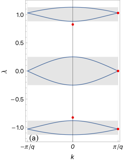
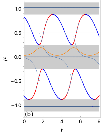
Figure 2: (Color online) Example of the spectrum for the $q=6$ system with the initial condition $a_{1}(=a_{4}):a_{2}(=a_{5}):a_{3}(=a_{6})=3:2:1$, while $b_{j}=0$. (a) The solid curves show $\lambda_{n}(k)$, and the red dots are the edge states at $t=0$. The shaded regions indicate the energies for which the Bloch states are allowed. (b) Time-evolution of the edge states in (a). The red and blue dots represent the edge states localized at the left and right ends, respectively, whereas the dark-blue dots forming straight lines are for the edge states within zero gaps that are prohibited to move. The shaded regions are the bulk bands. The small dark-blue and orange dots show the Berry phase $\Gamma_{n}$ (mod 1) of the lowest and middle bulk bands, respectively,

First, we consider a bulk system with $-\infty<l<\infty$. The $q$-periodicity of finite systems is enhanced to $q$-translational invariance in Eq. (23). Then, it follows from the Bloch theorem that $\tilde{\varphi}^{l}_{j}=\tilde{\varphi}_{ql+j}$ is simultaneously an eigenstate of the translation operator $\Delta$ as well as of $\hat{L}$. Thus, we set

$$\tilde{\varphi}^{l}_{j}=e^{ikql}\varphi_{j}(t,k),\quad(j=1,\dots,q)$$ (24)

where the Bloch function $\varphi_{j}(t,k)$ satisfies $\varphi_{j+q}(t,k)=\varphi_{j}(t,k)$. Note here that the $t$-dependence is explicitly written. Acting on the Bloch function, the Lax operator $\hat{L}(t)$ in (14) becomes the Bloch–Lax operator $L(t,k)$ in which the difference operators in $\hat{L}(t)$ are replaced by $\delta^{q}\rightarrow e^{iqk}$ and $\delta^{*q}\rightarrow e^{-iqk}$. We note that $|k|\leq\pi/q$. In Fig. 2 (a), an example of the bulk spectrum is shown, which is the system of $q=6$ particles with the initial condition $a_{1}=a_{4},a_{2}=a_{5},a_{3}=a_{6}\propto 3,2,1$. The spectrum comprises six bands, of which three pairs are gapless, forming three bands. This is because the minimum period is 3. Therefore, this feature is also true for a more generic system with $q=3N$ particles if a similar initial condition with period-3 is imposed. In this case, $N$ bulk bands appear in each shaded region in Fig. 2 (a) to form a single folded band. Thus, a total of three bands are separated by bulk gaps.

Next, we consider Eq. (23) under the open boundary condition. The exact solutions of the Toda lattice under the periodic boundary condition were obtained by using the edge states of $\hat{L}(t)$ Date and Tanaka (1976), where the edge states indicate the localized states at boundaries, which are absent in the bulk system. For numerical computations, a theory of edge states based on the Hermiticity of Hamiltonians, developed for quantum tight-binding Hamiltonians, is convenient Fukui (2020). Let $\tilde{\varphi}^{l}$ be defined on the semi-infinite line $l\geq 1$. The unit cell at $l=1$ is referred to as the left end. Equation (23) is explicitly given by the following recurrence relation: ${\cal K}\tilde{\varphi}^{l-1}+{\cal V}\tilde{\varphi}^{l}+{\cal K}^{T}\tilde{\varphi}^{l+1}=\lambda\tilde{\varphi}^{l}$. In particular, the initial equation for $l=1$ is given by:

$${\cal K}\tilde{\varphi}^{0}+{\cal V}\tilde{\varphi}^{1}+{\cal K}^{T}\tilde{\varphi}^{2}=\lambda\tilde{\varphi}^{1}.$$ (25)

Thus, to define the system for $l\geq 1$, ${\cal K}\tilde{\varphi}^{0}=0$ is imposed as the initial condition of the recurrence relation. Such vector $\tilde{\varphi}^{0}$ is generically given by $(\tilde{\varphi}^{0})^{T}=\left(\chi^{T},0\right)$, where $\chi$ is a $(q-1)$-vector. Now, assume a generalized Bloch state given by $\tilde{\varphi}^{l}=e^{iqKl}\tilde{\varphi}^{0}$ with a complex wavenumber $K=k+i\kappa$. Then, it is shown that not only is Eq. (23) satisfied for all $l\geq 1$, but also the Hermiticity of $L(t,k)$ is guaranteed at the boundary, as discussed in Ref. Fukui (2020). To be specific, the equation to be solved is

$$\left(\begin{array}[]{ccccc|c}b_{1}&a_{1}&&&&e^{-iqK_{n}}a_{q}\!\!\!\!\\ a_{1}&&&&&\\ &&\ddots&&&\\ &&&&a_{q-2}&\\ &&&a_{q-2}&b_{q-1}&a_{q-1}\\ \hline\cr\!\!e^{iqK_{n}}a_{q}\!\!\!\!\!\!&&&&a_{q-1}&b_{q}\\ \end{array}\right)\!\!\!\left(\begin{array}[]{c}\\ \\ \\ \!\!\chi_{n}\!\!\!\!\\ \\ \\ \hline\cr 0\end{array}\right)\!\!=\!\mu_{n}\!\!\left(\begin{array}[]{c}\\ \\ \\ \!\!\chi_{n}\!\!\!\!\\ \\ \\ \hline\cr 0\end{array}\right),$$ (46)

where $\mu_{n}(t,K_{n})$ denotes the energy of the edge states. Thus, it turns out that the eigenvalues of the edge states are those of the $(q-1)\times(q-1)$ reduced matrix of the Bloch–Lax operator in the above equation, and the last row gives the condition

$$e^{iqK_{n}}a_{q}\chi_{1n}+a_{q-1}\chi_{q-1,n}=0,$$ (47)

which determines $K_{n}=k_{n}+i\kappa_{n}$. In the present case, $k_{n}$ is restricted to $k_{n}=0,\pi$, and $\kappa_{n}$ is a generic real number depending on $t$. For the wave function $\tilde{\varphi}_{n}^{l}$ to be localized at the left end, $\kappa_{n}>0$ because $|\tilde{\varphi}_{n}^{l}|=e^{-q\kappa_{n}l}|\tilde{\varphi}^{0}|$. When $\kappa_{n}<0$, it cannot be an edge state at this end; instead, a state such as this is localized at the right end, if the system with the right end is considered (see Ref. Fukui (2020)). Thus, for a positive (negative) $\kappa$, the edge state is localized at the left (right) end.

We first examine how these edge states are embedded in the bulk band structure. In Fig. 2 (a), the edge states at $t=0$ are shown by red dots. Among the five edge states in the system with $q=6$ particles, three are fixed at the band touching points. Because the bulk spectrum is time independent, the energies of these edge states must also be. Thus, the other two edge states within the open gaps are responsible for the time evolution of the solution of the periodic Toda lattice. More generically, for a system of $q=3N$ particles with the same period-3 initial condition, there appear $3N-1$ edge states, among which $N-1$ states in each band are pinned at gapless points, and the remaining two edge states are located in the gaps.

Next, we show in Fig. 2 (b) the spectrum of the edge states as a function of $t$. The energies of the two edge states oscillate, whereas those of the three edge states are constant. The desired solution of $b_{q}(t)$ is obtained by simply using the time evolution of the edge states, such that footnote1

$$b_{q}(t)=\sum_{j=1}^{q}b_{j}(0)-\sum_{n=1}^{q-1}\mu_{n}(t).$$ (48)

Using the hyperelliptic abelian integrals and the solution to Jacobi’s inversion problem for the above equation, the exact solution can be written using the Riemann theta function Date and Tanaka (1976). This implies that the spectrum of the edge states $\mu_{n}(t)$ is sufficient to obtain the exact solution of the periodic Toda lattice. Here, let us turn our attention to the wave function $\varphi_{n}(t,k)$, which provides further information about the end at which the edge states are localized. Such a feature is irrelevant to the exact solutions, but informs us of the topological property of the solution. From Fig. 2 (b), we find that when $t=0$, the edge states are localized at the right end and when they touch the bulk bands under time evolution, they become localized at the opposite left end. Generically, the energies of the edge states oscillate as time evolves and when they touch the lower (upper) bulk band, the right (left) edge states change to the left (right) edge states. This is one of the characteristic properties of topological edge states.

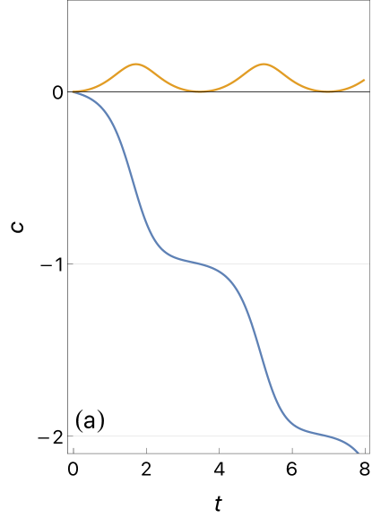
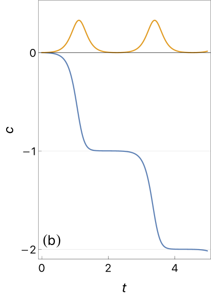
Figure 3: (Color online) (a) Berry fluxes $c(t)$ of the lowest and middle (orange) band for the same system as in Fig. 2. (b) the same system but for the initial condition, $a_{1}:a_{2}:a_{3}=20:2:1$, with a stronger nonlinearity than (a).

This feature of the Lax operator $L(t,k)$ is reminiscent of the Hamiltonian of the Thouless pump Thouless (1983), of which the Hamiltonian is generally a function of $t$ and $k$, $H(t,k)$ with $H(t+T_{0})=H(t,k)$ and $H(t,k+2\pi)=H(t,k)$. If the edge states of the Toda lattice have the same topological origin as the Thouless pump, they are guaranteed by the bulk topological invariants, the Chern numbers. This motivated us to compute the Berry phases and Berry fluxes associated with the Bloch wave function $\varphi(t,k)$ in Eq. (24).

First, we introduce the Berry phase:

$$\Gamma_{n}(t) =\frac{1}{2\pi i}\int_{-\pi}^{\pi}{\color[rgb]{0,0,0}dk}A_{n}(t,k),$$ (49)

where $A_{n}(t,k)$ is the Berry connection associated with the $n$-th band, which is defined as

$$A_{n}(t,k)=\varphi_{n}^{\dagger}(t,k)\partial_{k}\varphi_{n}(t,k).$$ (50)

The Berry phase describes the charge polarization in quantum systems Marzari et al. (2012). In Fig. 2 (b), the Berry phases $\Gamma_{n}(t)$ for the lowest and middle bands are shown modulo 1. We see that the Berry phase of the lowest band has a nontrivial winding number. Next, we introduce the Berry flux, defined as:

$$c_{n}(t)=\Gamma_{n}(t)-\Gamma_{n}(0).$$ (51)

This is equivalent to

$$c_{n}(t) =\frac{1}{2\pi i}\int_{0}^{t}\!\!dt\!\!\int_{-\pi}^{\pi}\!\!{\color[rgb]{0,0,0}dkF_{n}(t,k),}$$ (52)

where $F_{n}(t,k)$ is the Berry curvature, which is defined as

$$F_{n}(t,k)=\partial_{t}\varphi_{n}^{\dagger}(t,k)\partial_{k}\varphi_{n}(t,k)-{\rm c.c}.$$ (53)

For a periodic solution with a period $T_{0}$, $c_{n}(T_{0})$ is guaranteed to be an integer referred to as the Chern number.

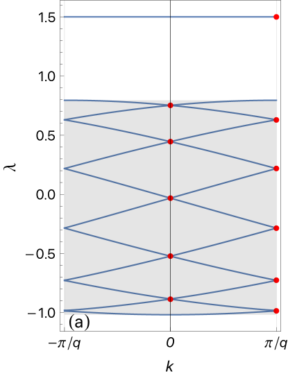
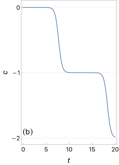
Figure 4: (Color online) (a) Bulk spectrum of the system with $q=12$ for the exact cnoidal wave solution. (b) Berry flux of (a).

In Fig. 3 (a), we show $c(t)$ for the system in Fig. 2 calculated by the method developed in Ref. Fukui et al. (2005). We see that for just one period, $c$ changes by $-1$. This implies that the Chern number of the lowest band is $c=-1$. This bulk topological invariant guarantees the existence and stability of the edge states in the lower gap. By contrast, the second band does not have nonzero Chern numbers; hence, it is a topologically trivial band. Thus, the edge states in the upper gap are topologically stable, because they are associated with the sum of the Chern numbers below the gap $-1+0=-1$ Hatsugai (1993b, a). For other multiband systems not shown here, we also observe similar behavior of the edge states in open gaps. The stability of the edge states indicates the stability of the solutions of the Toda lattice; thus, we conclude that the solutions of the periodic Toda lattice are topologically stable. Remarkably, when substantial nonlinearity exists, as shown in Fig. 3 (b), $c(t)$ plateaus at the integers $c=-n$. From the distance between these plateaus, we can easily determine the Chern numbers for one period of the solutions for (3).

This feature is also true for the cnoidal wave of the periodic Toda lattice Toda (1967a, b). In Fig. 4, we show the bulk spectrum and Berry flux of the $q=12$ system for the exact single-mode cnoidal wave solution with very large nonlinearity. As expected, this is a two-band system Date and Tanaka (1976), and the Berry flux exhibits very sharp plateaus, from which we obtain the Chern number of $c=-1$ for one period.

This observation raises the question of whether the Bloch–Lax operator $L(t,k)$ allows topologically trivial solutions, such as for the Thouless pump. In the Thouless pump, not only the edge states but also the bulk states depend on time, such that at a certain time, gap-closing may occur, resulting in a transition between the nontrivial and trivial phases Nakajima et al. (2016); Lohse et al. (2016). However, in the present case, the bulk spectrum is time independent, implying that such a point-like gap closing phenomenon is absent. Therefore, it is natural to expect the Lax operator to have no trivial phase; hence, the cnoidal wave and more generic solutions of the periodic Toda lattice are topologically stable.

In conclusion, we revealed the topological properties of the edge states that are used to obtain the exact solution of the periodic Toda lattice. We attributed the stability of nontopological solitons to the topological properties of the Lax operator.

This work was supported in part by a Grant-in-Aid for Scientific Research (22K03448) from the Japan Society for the Promotion of Science.

References

- Toda (1967a) M. Toda, J. Phys. Soc. Jpn 22, 431 (1967a), URL https://doi.org/10.1143/JPSJ.22.431.
- Toda (1967b) M. Toda, J. Phys. Soc. Jpn 23, 501 (1967b), URL https://doi.org/10.1143/JPSJ.23.501.
- Lax (1968) P. D. Lax, Comm. Pure Appl. Math. 21, 467 (1968), eprint https://onlinelibrary.wiley.com/doi/pdf/10.1002/cpa. 3160210503, URL https://onlinelibrary.wiley.com/doi/abs/10.1002/cpa.3160210503.
- Flaschka (1974a) H. Flaschka, Prog. Theor. Phys. 51, 703 (1974a), ISSN 0033-068X, eprint https://academic.oup.com/ptp/article-pdf/51/3/703/5304458/51-3-703.pdf, URL https://doi.org/10.1143/PTP.51.703.
- Kac and van Moerbeke (1975) M. Kac and P. van Moerbeke, Proc. Natl. Acad. Sci. U.S.A 72, 1627 (1975).
- Date and Tanaka (1976) E. Date and S. Tanaka, Prog. Theor. Phys. 55, 457 (1976), URL https://doi.org/10.1143/PTP.55.457.
- Hatsugai (1993a) Y. Hatsugai, Phys. Rev. Lett. 71, 3697 (1993a), URL http://link.aps.org/doi/10.1103/PhysRevLett.71.3697.
- Hatsugai (1993b) Y. Hatsugai, Phys. Rev. B 48, 11851 (1993b), URL https://link.aps.org/doi/10.1103/PhysRevB.48.11851.
- Altland and Zirnbauer (1997) A. Altland and M. R. Zirnbauer, Phys. Rev. B 55, 1142 (1997), URL http://link.aps.org/doi/10.1103/PhysRevB.55.1142.
- Zirnbauer (1996) M. R. Zirnbauer, J. Math. Phys. 37, 4986 (1996), URL https://doi.org/10.1063/1.531675.
- Schnyder et al. (2008) A. P. Schnyder, S. Ryu, A. Furusaki, and A. W. W. Ludwig, Phys. Rev. B 78, 195125 (2008), URL http://link.aps.org/doi/10.1103/PhysRevB.78.195125.
- Thouless et al. (1982) D. J. Thouless, M. Kohmoto, M. P. Nightingale, and M. den Nijs, Phys. Rev. Lett. 49, 405 (1982), URL http://link.aps.org/doi/10.1103/PhysRevLett.49.405.
- Kohmoto (1985) M. Kohmoto, Ann. Phys. 160, 343 (1985).
- Thouless (1983) D. J. Thouless, Phys. Rev. B 27, 6083 (1983), URL http://link.aps.org/doi/10.1103/PhysRevB.27.6083.
- Nakajima et al. (2016) S. Nakajima, T. Tomita, S. Taie, T. Ichinose, H. Ozawa, L. Wang, M. Troyer, and Y. Takahashi, Nat. Phys. 12, 296 (2016), URL http://dx.doi.org/10.1038/nphys3622.
- Lohse et al. (2016) M. Lohse, C. Schweizer, O. Zilberberg, M. Aidelsburger, and I. Bloch, Nat. Phys. 12, 350 (2016), URL http://dx.doi.org/10.1038/nphys3584.
- Kaup (1976) D. J. Kaup, SIAM J. Appl. Math. 31, 121 (1976), eprint https://doi.org/10.1137/0131013, URL https://doi.org/10.1137/0131013.
- Flaschka (1974b) H. Flaschka, Phys. Rev. B 9, 1924 (1974b), URL https://link.aps.org/doi/10.1103/PhysRevB.9.1924.
- Fukui (2020) T. Fukui, Phys. Rev. Res. 2, 043136 (2020), URL https://link.aps.org/doi/10.1103/PhysRevResearch.2.043136.
- (20) For variables other than , choose the appropriate unit cell; for example, that surrounded by the dashed square in Fig. 1, from which one can compute .
- Marzari et al. (2012) N. Marzari, A. A. Mostofi, J. R. Yates, I. Souza, and D. Vanderbilt, Rev. Mod. Phys. 84, 1419 (2012), URL http://link.aps.org/doi/10.1103/RevModPhys.84.1419.
- Fukui et al. (2005) T. Fukui, Y. Hatsugai, and H. Suzuki, J. Phys. Soc. Jpn. 74, 1674 (2005), URL http://dx.doi.org/10.1143/JPSJ.74.1674.