Universal Slow Dynamics of Chemical Reaction Networks

Abstract

Understanding the emergent behavior of chemical reaction networks (CRNs) is a fundamental aspect of biology and its origin from inanimate matter. A closed CRN monotonically tends to thermal equilibrium, but when it is opened to external reservoirs, a range of behaviors is possible, including transition to a new equilibrium state, a non-equilibrium state, or indefinite growth. This study shows that slowly driven CRNs are governed by the conserved quantities of the closed system, which are generally far fewer in number than the species. Considering both deterministic and stochastic dynamics, a universal slow dynamics equation is derived with singular perturbation methods, and is shown to be thermodynamically consistent. The slow dynamics is highly robust against microscopic details of the network, which may be unknown in practical situations. In particular, non-equilibrium states of realistic large CRNs can be sought without knowledge of bulk reaction rates. The framework is successfully tested against a suite of networks of increasing complexity and argued to be relevant in the treatment of open CRNs as chemical machines.

I Introduction

The goal of theory for complex systems is often to reduce the number of degrees of freedom from a large intractable number down to something manageable, whose dynamics can then be understood intuitively. Ideally, such a reduction should be principled, mathematically well-controlled, and lead to a description in terms of universal effective variables. This challenge is especially acute in the biosciences where dizzying complexity is the norm. We address it for chemical reaction networks (CRN), which provide the substrate for biochemistry and hence biology.

Model reduction for CRNs has a long history Okino98 ; Radulescu12 ; Snowden17 . Since CRNs often contain a wide range of timescales, many reduction methods exploit this by quasi-equilibrium or quasi-steady-state approximations Schneider00 . However, existing theories employ different reductions for each particular CRN, thus not leading to any universal description. This may be sufficient for detailed analysis of a particular system, but makes cross-system analysis difficult and hinders unification of diverse phenomena. Moreover, these approaches work at the level of the rate equations, ignoring stochastic effects known to be important in biochemistry Bressloff17 . They may also fail to respect thermodynamic constraints Peng23 .

Here we take a different route, grounded in hydrodynamics, a branch of condensed matter physics Chaikin00 . The starting point for hydrodynamics is the observation that molecular timescales, on the order of picoseconds, are miniscule compared to macroscopic forcing timescales. Thus most degrees of freedom relax very rapidly to a state of local thermodynamic equilibrium. However, over macroscopic distances, forcing conditions can differ, thus leading to different local equilibria. In such a hydrodynamic limit in which forcing is slow in time and gradual in space, only a subset of degrees of freedom, dictated by symmetries and conservation laws, are important. Indeed, conserved quantities are precisely those whose densities need to be tracked, while the other degrees of freedom relax quickly and can be neglected . Conventional continuum theories for fluids, elastic solids, liquid crystals, and others are all of this type, differing only in the assumed symmetries Chaikin00 .

This vantage is natural for chemical reaction networks, since individual reactions conserve the number of each element, leading to a large number of conservation laws. While previous and ongoing work on CRNs in the mathematical literature has also exploited conservation laws Ren06 ; Lee10 ; Desoeuvres22 , such approaches do not incorporate thermodynamic constraints, nor do they yield a universal description. Instead we combine notions from hydrodynamics with stochastic thermodynamics Schmiedl07 ; Seifert12 ; Van-den-Broeck13 ; Wachtel18 ; Wachtel22 ; Avanzini23 , building thermodynamic consistency in from the beginning. This is useful to quantify CRNs as chemical machines, as will be discussed later Wachtel22 ; Avanzini23 .

In particular we consider slowly driven well-mixed physical CRNs, and show that they are governed by conservation of elements, similar to hydrodynamic theories. We derive a universal slow dynamics equation, (25) below, that can be applied to generic slowly-driven CRNs. For a CRN with $N$ species and $E$ elements, the reduced theory generally involves only $E$ variables. We work at the large-deviations level of the particle number distribution, thus incorporating the leading stochastic effects.

This article is organized as follows. First, we define our CRN, emphasizing the role of microscopic reversibility. Then we analyze the rate equation in the slowly-driven setting, showing that a naive perturbation expansion breaks down. This is cured by a singular perturbation theory, which leads to the slow dynamics equation. We then extend the theory to include stochastic effects, and test our theory with numerical simulations, showing its broad utility. Finally we show how the theory can be extended to initial states that are far from equilibrium.

Species are indexed with $i,j,\ldots$ while reactions are indexed with $\alpha,\beta,\ldots$. We use vector notation whenever possible. For example, stoichiometric coefficients $p_{i\alpha}$ and $q_{i\alpha}$ are also written as $\vec{p}_{\alpha}$ and $\vec{q}_{\alpha}$. All contractions are explicitly indicated by dots. In CRNs, many functions appear that act component-wise on different species. We write $[\vec{f}({\vec{n}})\vec{g}({\vec{n}})\cdots]$ for the vector in species space whose components are $f_{j}({\vec{n}})g_{j}({\vec{n}})\cdots$. For example, $[{\vec{n}}^{eq}e^{\vec{c}}]$ has components $n_{j}^{eq}e^{c_{j}}$, etc. When such expressions are considered as diagonal matrices, we double the brackets, i.e. $[[\vec{f}]]$ is the matrix with elements $\delta_{ij}f_{i}$. To sum or multiply over all species we write $\sum[\vec{f}]$ and $\prod[\vec{f}]$, respectively. We also apply this notation to component-wise vectors over reactions.

II Slowly driven chemical reaction networks

We define a physical CRN as follows. We have $N$ species $X_{i}$, interacting with $M$ reactions $\alpha$, split into the core and the boundary interactions. Write a general core reaction as

$$\sum_{i}p_{i\alpha}X_{i}\rightleftharpoons\sum_{i}q_{i\alpha}X_{i},$$ (1)

where $p_{i\alpha}$ and $q_{i\alpha}$ are the stoichiometric coefficients for the molecular species as reactant and product, respectively.

The number of moles of all species are collected in a vector ${\vec{n}}$. Quantum mechanics requires that if a reaction $\alpha$ occurs with rate $k^{+}_{\alpha}$, then its corresponding backward reaction must occur, with rate $k^{-}_{\alpha}$. As a condition for existence of thermal equilibrium, these rates are not independent but constrained in ratio to satisfy

$$\frac{k^{+}_{\alpha}({\vec{n}})}{k^{-}_{\alpha}({\vec{n}})}=e^{-\frac{1}{RT}(\Delta G)_{\alpha}},$$ (2)

where $(\Delta G)_{\alpha}=(\vec{q}_{\alpha}-\vec{p}_{\alpha})\cdot\vec{G}({\vec{n}})$ is the difference in molar Gibbs free energy between products and reactants. (2) is known as local detailed balance Van-den-Broeck13 ; Polettini14 ; Rao16 ; Wachtel22 , or microscopic reversibility Astumian18 . Importantly, it does not require or imply that the CRN be in thermal equilibrium or close to it. In a physical CRN, we require that all reactions in the core of the system satisfy (2). For the boundary interactions, which force the system, we consider intake and degradation pairs

$$X_{i}^{\mathscr{C}}\rightleftharpoons X_{i},$$ (3)

with rates $\epsilon r_{i}^{+}$ and $\epsilon r_{i}^{-}$, respectively, where $\epsilon$ is a dimensionless constant. The ${\mathscr{C}}$ decoration denotes a chemostat.

The CRN is slowly driven when $\epsilon\ll 1$, meaning that all reservoir interactions are slow compared to internal reactions. This condition is quite natural. Indeed, bulk reaction rates are proportional to the volume of the system, $\Omega$, while boundary rates are proportional to the surface area, $\partial\Omega$. Their ratio $L\equiv\Omega/\partial\Omega$ is a length, on the order of the linear dimension of the system. To obtain the dimensionless parameter $\epsilon$, this must be compared with a microscopic length. For example, in the case of passive diffusion across a membrane with similar concentrations on both sides of the membrane, the microscopic length is $\delta\approx D/(k_{0}d)$ where $d$ is the membrane thickness and $D$ is the diffusion constant . $\epsilon$ can be defined as $\epsilon=\delta/L$, which for typical values $d\sim 10nm$ and $D\sim 10^{-9}m^{2}/s$ gives $\epsilon\sim 10^{-14}m/L$, which is small even for microscopic systems. This example furthermore illustrates that the slow driving condition can be avoided if systems have an anomalously large surface area (as in mitochondria), if diffusion is active (as in the sodium-potassium pump), if large concentration differences are held across the membrane, or if important bulk reactions are significantly slower than $k_{0}$.

As a consequence of slow driving, after an initial relaxation the system will be close to some thermal equilibrium state. However, over long timescales it can have a non-trivial dynamics near evolving equilibria, just as a fluid that is stirred or poured will transition through a series of near-equilibria, described in that case by the Navier-Stokes equations. Our main result is an evolution equation for the slow degrees of freedom, which, as we show, correspond to conserved quantities, in precise analogy with hydrodynamics. For a generic large CRN, the conserved quantities are the number of each element (H,C,O,..) and number of free electrons, if ions are present.

The local detailed balance condition (2) can also be derived microscopically. Indeed, modern transition rate theory Gilbert90 predicts from first principles

$$k^{+}_{\alpha}({\vec{n}})=ke^{-\frac{1}{RT}(\delta G)_{\alpha}({\vec{n}})},$$ (4)

where $(\delta G)_{\alpha}({\vec{n}})=G_{A_{\alpha}}-\sum_{i}p_{i\alpha}G_{i}({\vec{n}})$ is the difference in molar Gibbs free energy between the activated complex and the reactants, and $k=\Omega c^{\circ}k_{0}$ in terms of $k_{0}=1/(2\pi\beta\hbar)\approx 6\times 10^{12}$ Hz at 300K. Here $\Omega$ is the system volume, assumed to be dominated by the solvent, and $c^{\circ}$ is standard concentration 1 mol/L. (4) holds for both forward and backward reactions, mutatis mutandis, so that (2) is satisfied.

For ideal dilute solutions, the free energies (chemical potentials) for each species take the form

$$G_{i}({\vec{n}})=\mu^{\circ}_{i}+RT\log(n_{i}/c^{\circ}\Omega)=RT\log(n_{i}/n_{i}^{eq})$$ (5)

where $\mu^{\circ}_{i}$ is the chemical potential in standard conditions, and $n_{i}^{eq}=\Omega c^{\circ}e^{-\mu^{\circ}_{i}/RT}$. The forward reaction rates are thus proportional to $\prod_{i}(n_{i}/c^{\circ}\Omega)^{p_{i\alpha}}$, which is the law of mass action. The flux of reaction $\alpha$ is

$$J_{\alpha}({\vec{n}}) =k^{+}_{\alpha}({\vec{n}})-k^{-}_{\alpha}({\vec{n}})$$

$$=ke^{-G_{A_{\alpha}}/RT}\left(\prod\left[({\vec{n}}/{\vec{n}}^{eq})^{\vec{p}_{\alpha}}\right]-\prod\left[({\vec{n}}/{\vec{n}}^{eq})^{\vec{q}_{\alpha}}\right]\right)$$ (6)

We can write the rates of reservoir interactions in the form

$$r_{i}^{+}=r_{i}z^{\mathscr{C}}_{i},\quad r_{i}^{-}(n_{i})=r_{i}n_{i}/\Omega,$$ (7)

where $z_{i}^{\mathscr{C}}$ is the molar concentration of species $i$ in its reservoir; in general this can be time-dependent. The numbers $r_{i}$ have units of rate per mole times volume, while the factors $z^{\mathscr{C}}_{i}$ and $n_{i}$ account for the law of mass action.

Note that to precisely distinguish energy from entropy, and hence to unambiguously identify heat flows, requires a microscopic Hamiltonian Schmiedl07 . However, by comparing (2) to our rate parametrization for reservoir interactions, we can write

$$\frac{r_{i}^{+}}{r_{i}^{-}(n_{i})}=\frac{\epsilon r_{i}z_{i}^{\mathscr{C}}}{\epsilon r_{i}n_{i}/\Omega}=e^{-\frac{1}{RT}(G_{i}({\vec{n}})-W_{i})},$$ (8)

where $W_{i}$ is the work done by the reservoir in one intake reaction. This identifies $W_{i}=\mu^{c^{\circ}}_{i}+RT\log(z_{i}^{\mathscr{C}}/c^{\circ})$, which is just the chemical potential of species $i$ at the reservoir concentration, as expected.

To quantify how far a CRN is from equilibrium, we measure the entropy production rate

$$T\dot{S}=TR\sum\left[(\vec{k}^{+}-\vec{k}^{-})\log\frac{\vec{k}^{+}}{\vec{k}^{-}}\right]\geq 0$$ (9)

Define the N by M stoichiometric matrix $\mathbb{S}=[\mathbb{S}^{0}\;\mathbb{S}^{\mathscr{C}}]$ where $\mathbb{S}^{0}_{i\alpha}=q_{i\alpha}-p_{i\alpha}$ are the stoichiometric coefficients for the core reactions, and $\mathbb{S}^{\mathscr{C}}_{i\alpha}=+1$ when $\alpha$ corresponds to a reservoir of species $i$, and 0 otherwise. Using local detailed balance, the entropy production can be rewritten as

$$T\dot{S} =-\sum\left[(\vec{k}^{+}-\vec{k}^{-})\left(\mathbb{S}^{T}\cdot\vec{G}({\vec{n}})-(\mathbb{S}^{{\mathscr{C}}})^{T}\cdot\vec{W}\right)\right]$$

$$=-\vec{G}({\vec{n}})\cdot\mathbb{S}\cdot(\vec{k}^{+}-\vec{k}^{-})+\vec{W}\cdot(\vec{r}^{+}-\vec{r}^{-}),$$ (10)

which will be useful below.

Note that in our setup, each species present in a reservoir has two concentrations: its dynamical concentration in the system, $n_{j}/\Omega$, and its concentration in the reservoir, denoted $z_{j}^{\mathscr{C}}$. These only become equal, in general, when the reservoir rate $r_{j}\to\infty$ (although we will see other situations below where they equilibrate). Thus having a fully chemostatted species, as often considered in the literature, is a strong driving limit, since the corresponding species must be added or removed faster than any reaction rate in the system, to maintain its constant concentration. Our setup more naturally respects real-world constraints.

III Deterministic analysis

To illustrate our approach, we first consider the rate equations for our model; later we will generalize our results to include stochastic effects. The rate equations are

$$\partial_{t}{\vec{n}}=\mathbb{S}\cdot{\vec{J}}({\vec{n}})$$ (11)

where ${\vec{J}}$ is the vector of reaction fluxes. Separating the reactions into core and boundary, this becomes

$$\partial_{t}{\vec{n}}=\mathbb{S}^{0}\cdot{\vec{J}}^{\;0}({\vec{n}})+\epsilon\;[\;\vec{r}\;(\vec{z}^{\mathscr{C}}-{\vec{n}}/\Omega)],$$ (12)

where ${\vec{J}}^{\;0}({\vec{n}})$ is the reaction flux vector for core reactions, and where $r_{j}=0$ if there is no reservoir for species $j$. (12) suggests a perturbative solution in $\epsilon:{\vec{n}}={\vec{n}}^{0}+\epsilon{\vec{n}}^{1}+\ldots$. At leading order $\partial_{t}{\vec{n}}^{0}=\mathbb{S}^{0}\cdot{\vec{J}}^{0}({\vec{n}}^{0})$, which describes a closed system. The system monotonically tends to thermal equilibrium, described by ${\vec{J}}^{0}({\vec{n}}^{0})=0$. The general steady-state solution is

$${\vec{n}}^{0}=[{\vec{n}}^{eq}e^{{\vec{c}}}]=\Omega c^{\circ}[e^{-\vec{\mu}^{\circ}/RT}e^{{\vec{c}}}]$$ (13)

where we must have $(\mathbb{S}^{0})^{T}\cdot{\vec{c}}=0$. Such vectors ${\vec{c}}$ are the conserved quantities of the closed CRN. To see this more explicitly, let ${\vec{Y}}=(e^{-},H,C,O,\ldots)$ be a vector of elements that appear in the CRN, and write each species as an abstract sum of elements

$$X_{j}=\sum_{e}\zeta_{je}Y_{e},$$ (14)

defining the atomic matrix $\zeta$. Let there be $E$ elements so that $\zeta$ is an N by E matrix. The condition for conservation of element $e$ at reaction $\alpha$ is

$$0=\sum_{j}q_{j\alpha}\zeta_{je}-\sum_{j}p_{j\alpha}\zeta_{je}=\big{(}(\mathbb{S}^{0})^{T}\cdot\zeta\big{)}_{\alpha e},$$ (15)

showing that $\vec{\zeta}_{e}$ is a conserved quantity. If the columns of $\zeta$ are a basis for this space, then we can write

$${\vec{c}}=\zeta\cdot{\vec{\eta}},$$ (16)

where ${\vec{\eta}}$ is a vector in element space. Comparing with (13) we see that nonzero ${\vec{c}}$ is equivalent to shifting chemical potentials by

$$\vec{\mu}^{\circ}\to\vec{\mu}^{\circ}-RT\zeta\cdot{\vec{\eta}}.$$ (17)

Therefore $RT{\vec{\eta}}$ corresponds to a shift in the chemical potential of elements. ( In our rate parametrization a full transformation would require also shifting activation energies by $G_{A_{\alpha}}\to G_{A_{\alpha}}-RT\vec{p_{\alpha}}\cdot\zeta\cdot{\vec{\eta}}$.) It acts as a ‘tilt’ in the free energy landscape, which fixes the number of each element as

$$\vec{y}=\zeta^{T}\cdot{\vec{n}}=\zeta^{T}\cdot[{\vec{n}}^{eq}e^{\zeta\cdot{\vec{\eta}}}]+\mathscr{O}(\epsilon)$$ (18)

Although this gives $E$ equations in $E$ unknowns, they cannot be explicitly solved for ${\vec{\eta}}$.

At the next order we have

$$\partial_{t}{\vec{n}}^{1}=(\mathbb{S}^{0})\cdot\left.\big{(}\partial{\vec{J}}^{\;0}/\partial{\vec{n}}\big{)}\right|_{{\vec{n}}^{0}}\cdot{\vec{n}}^{1}+\left.[\vec{r}(\vec{z}^{\mathscr{C}}-{\vec{n}}/\Omega)]\right|_{{\vec{n}}^{0}}$$ (19)

If we multiply by $\zeta^{T}$ we get

$$\partial_{t}\zeta^{T}\cdot{\vec{n}}^{1}=\zeta^{T}\cdot[\vec{r}(\vec{z}^{\mathscr{C}}-{\vec{n}}^{0}/\Omega)],$$ (20)

which expresses element balance. This equation can be directly integrated. For simplicity assume that the reservoirs are independent of time. Then after an initial relaxation we will have

$$\zeta^{T}\cdot{\vec{n}}^{1}(t)\sim t\zeta^{T}\cdot[\vec{r}(\vec{z}^{\mathscr{C}}-{\vec{n}}^{0}(\infty)/\Omega)],$$ (21)

which diverges at large $t$. After a time $t\sim 1/\epsilon$ we will have $\epsilon{\vec{n}}^{1}\sim{\vec{n}}^{0}$ and the perturbation series breaks down. Thus the slow driving limit $\epsilon\to 0$ is singular. This is not specific to our boundary conditions or simplifying assumptions, but is completely generic.

This mathematical singularity has a simple physical interpretation: when the system is open to reservoirs, elements can be exchanged with the environment. Over a long time scale $t\sim 1/\epsilon$, the relevant thermal equilibrium state can be completely different from its initial value. Fortunately, this suggests a cure to the long-time divergence: we need to consider a multiple-scales asymptotic analysis Bender99 ; Hinch91 . We introduce the slow time $\tau=t\epsilon$, so-named because $\tau\sim\mathscr{O}(1)$ when $t\sim 1/\epsilon$, and replace the time derivative by

$$\frac{\partial}{\partial t}\to\frac{\partial}{\partial t}+\epsilon\frac{\partial}{\partial\tau}$$

The leading order solution remains the same, except that the coefficients ${\vec{\eta}}$ get promoted to functions of the slow time, capturing their evolution on long time scales. The $\mathscr{O}(\epsilon)$ equation becomes

$$\partial_{\tau}{\vec{n}}^{0}+\partial_{t}{\vec{n}}^{1}=(\mathbb{S}^{0})\cdot\left.\big{(}\partial{\vec{J}}^{\;0}/\partial{\vec{n}}\big{)}\right|_{{\vec{n}}^{0}}\cdot{\vec{n}}^{1}+[\vec{r}(\vec{z}^{\mathscr{C}}-{\vec{n}}^{0}/\Omega)]$$

Multiplying by $\zeta^{T}$ we have

$$\zeta^{T}\cdot\partial_{\tau}{\vec{n}}^{0}+\zeta^{T}\cdot\partial_{t}{\vec{n}}^{1}=\zeta^{T}\cdot[\vec{r}(\vec{z}^{\mathscr{C}}-{\vec{n}}^{0}/\Omega)]$$ (22)

At this order, the divergences are cured if we impose

$$\zeta^{T}\cdot\partial_{\tau}{\vec{n}}^{0}=\zeta^{T}\cdot[\vec{r}(\vec{z}^{\mathscr{C}}-{\vec{n}}^{0}/\Omega)]$$ (23)

which are the slow dynamics equations. As shown below, these same equations will remain valid for stochastic dynamics. We have $E$ equations in $E$ DOF. More explicitly,

$$\sum_{j,e^{\prime}}\zeta_{je}n_{j}^{eq}e^{\sum_{e}\zeta_{je}\eta_{e}}\zeta_{je^{\prime}}\partial_{\tau}\eta_{e^{\prime}}=\sum_{j}\zeta_{je}r_{j}(z_{j}^{\mathscr{C}}-n_{j}^{eq}e^{\sum_{e}\zeta_{je}\eta_{e}}/\Omega)$$ (24)

Defining the matrix $M({\vec{\eta}})=\zeta^{T}\cdot[[{\vec{n}}^{eq}e^{\zeta\cdot{{\vec{\eta}}}}]]\cdot\zeta$ and the external flux ${\vec{J}}^{\mathscr{C}}({\vec{\eta}})=[\vec{r}(\vec{z}^{\mathscr{C}}-{\vec{n}}^{eq}e^{\zeta\cdot{\vec{\eta}}}/\Omega)]$ we can write this as

$$M\cdot\partial_{\tau}{\vec{\eta}}=\zeta^{T}\cdot{\vec{J}}^{\mathscr{C}},$$ (25)

which is our main result. (25) is a strongly nonlinear system of equations governing the evolution of near-equilibrium states in a slowly driven CRN. The core CRN can be completely arbitrary, as long as it is detailed balanced. The reservoirs can be forced arbitrarily on the slow time scale; that is, $\vec{r}$ and ${\vec{n}}^{\mathscr{C}}$ can be arbitrary functions of $\tau$.

Note that $\zeta^{T}\cdot{\vec{n}}$ is simply the number of moles of each element; thus from (23) the slow dynamics equation is simply the conservation law for elements, which under slowly-driven conditions gives a closed set of equations. Remarkably, the number of degrees of freedom is reduced from $N$ down to $E$. Moreover, these slow DOF are not arbitrary but are easily interpretable and universal across different CRNs.

If some elements appear in the CRN but not in any reservoirs, then their concentrations are clearly conserved at their initial values; in this case the corresponding entries of the slow dynamics equations can be immediately solved, leading to a further reduction in the number of evolving DOF.

(25) is also remarkably universal in form: it does not depend on any activation energies in the core, and steady states are also independent of core chemical potentials. It can thus be applied to poorly characterized CRNs where only the stoichiometry, chemical potentials, and reservoir interactions are known.

The slow dynamics equation describes the dissipative dynamics through near-equilibrium states. In SI, we show that at leading order the dissipation depends only on the slow dynamics, and not also on ${\vec{n}}^{1}$ as might naively be expected. In particular it takes a simple form

$$T\dot{S} =\vec{W}\cdot(\vec{r}^{+}-\vec{r}^{-})+\mathscr{O}(\epsilon^{2})$$ (26)

which can be evaluated on the solution of (25).

Above, we use the elements as the conserved quantities of the CRN. In full generality, one can replace the matrix $\zeta$ above with a basis of conserved quantities defined from the relation $\mathbb{S}^{0}\cdot\zeta=0$; these are called ‘moieties’ and for small CRNs can differ from the elements De-Martino09 . For example, if carbon and oxygen only appear in the CRN in multiples of CO, then their individual concentrations, while both conserved, are degenerate. All our developments hold if $\zeta$ is a basis of conserved moieties rather than elements, but for clarity of exposition, we continue to use the terminology of elements. Moreover, for large CRNs where we expect our theory to be of interest, there are generally no conserved quantities besides the elements.

IV Stochastic analysis

We now extend our results to include stochastic effects; in a first reading, this section can be omitted. We begin from the Doi-Peliti path integral formulation Doi76 ; Peliti85 , which is an exact rewriting of the chemical master equation for the full counting statistics $\mathbb{P}({\vec{n}},t)$. For a self-contained review see De-Giuli22b . The CRN is specified by the quasi-Hamiltonian (or Liouvillian) $H=H_{0}+\epsilon H_{\mathscr{C}}$ with

$$H_{0}({\vec{n}},\vec{\nu}) =\sum_{\alpha}k_{\alpha}\left\{\quantity(e^{\vec{\nu}\cdot\quantity(\vec{q}_{\alpha}-\vec{p}_{\alpha})}-1)\prod\left[\quantity(\frac{{\vec{n}}}{{\vec{n}}^{eq}})^{\vec{p}_{\alpha}}\right]\right.$$

$$\left.+\quantity(e^{-\vec{\nu}\cdot\quantity(\vec{q}_{\alpha}-\vec{p}_{\alpha})}-1)\prod\left[\quantity(\frac{{\vec{n}}}{{\vec{n}}^{eq}})^{\vec{q}_{\alpha}}\right]\right\}$$ (27)

$$H_{\mathscr{C}}({\vec{n}},\vec{\nu}) =\sum\left[\vec{r}(e^{-\vec{\nu}}-1){\vec{n}}/\Omega+\vec{r}(e^{\vec{\nu}}-1)\vec{z}^{\mathscr{C}}\right].$$ (28)

The $\vec{\nu}$ variables act as a per-species bias. As explained in SI, in the macroscopic regime where particle numbers are large the leading behavior of $\rho\equiv\log\mathbb{P}$ satisfies a Hamilton-Jacobi equation Kubo73 ; Kitahara75 ; Smith20

$$\frac{\partial\rho({\vec{n}},t)}{\partial t}=H({\vec{n}},-\nabla_{{\vec{n}}}\rho({\vec{n}},t)).$$ (29)

(29) goes beyond the Gaussian approximation as it includes rare trajectories between different attractors, if they exist. In the slowly driven case, we require that $\Omega c^{\circ}\epsilon\gg 1$, which ensures that the slow driving is more relevant than finite-size fluctuations from the bulk of the system.

Let $\{\vec{c}_{x}\}_{x=1}^{E}$ be a basis of the left kernel (or cokernel) of the stoichiometric matrix $\mathscr{K}=\operatorname{coker}\mathbb{S}$, i.e., this system has $E$ conserved quantities. We solve (29) under the initial condition

$$\rho({\vec{n}},t=0) =\sum\left[{\vec{n}}\log\vec{\lambda}^{(0)}-\vec{\lambda}^{(0)}-{\vec{n}}\log\frac{{\vec{n}}}{e}\right],$$ (30)

$$\vec{\lambda}^{(0)} =[{\vec{n}}^{eq}e^{{\vec{c}}^{(0)}}],$$ (31)

where $\vec{c}^{(0)}$ is an arbitrary vector in $\mathscr{K}$. This is a large deviation function of a Poisson distribution in the limit $n_{i}\to\infty$

$$\mathbb{P}({\vec{n}},0)=\prod\left[\frac{\quantity(\vec{\lambda}^{(0)})^{{\vec{n}}}e^{-\vec{\lambda}^{(0)}}}{({\vec{n}}/e)^{{\vec{n}}}}\right]\sim\prod\left[\frac{\quantity(\vec{\lambda}^{(0)})^{{\vec{n}}}e^{-\vec{\lambda}^{(0)}}}{{\vec{n}}!}\right]$$

with means $\vec{\lambda}^{(0)}$.

Introducing the two time variables $t$ and $\tau=\epsilon t$ as in the previous subsection, (29) is rewritten as

$$\quantity(\partialderivative{t}+\epsilon\partialderivative{\tau})\rho({\vec{n}},t,\tau) =H({\vec{n}},-\nabla_{{\vec{n}}}\rho({\vec{n}},t,\tau))$$

with

$$\rho({\vec{n}},t=0,\tau=0) =\sum_{i}\quantity[n_{i}\log\lambda_{i}^{(0)}-\lambda_{i}^{(0)}-n_{i}\log\frac{n_{i}}{e}].$$

We expand the solution of this equation as $\rho({\vec{n}},t,\tau)=\rho_{0}({\vec{n}},t,\tau)+\epsilon\rho_{1}({\vec{n}},t,\tau)+\cdots$. The leading equation is

$$\partialderivative{t}\rho_{0}({\vec{n}},t,\tau)=H_{0}({\vec{n}},-\nabla_{{\vec{n}}}\rho_{0}({\vec{n}},t,\tau)),$$

which is already solved by the initial condition. We cannot determine the $\tau$-dependence of the vector $\vec{c}(\tau)\in\mathscr{K}$ at this order.

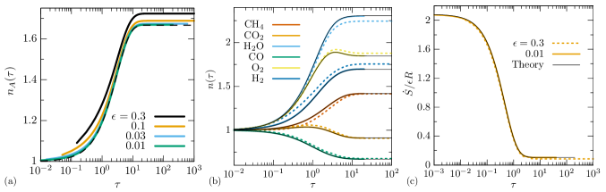
Figure 1: The slow dynamics equation tracks solutions to the full rate equations, even through non-equilibrium processes. In (a) the ABC model is shown with numerical solutions (solid), and the slow dynamics equation (dashed) for a range of $\epsilon$. In (b,c), the methane combustion model is shown for numerical solutions with $\epsilon=0.3$ (dashed) and $\epsilon=0.01$ (solid, colored) and compared to the result from the slow dynamics equation (solid, black). These results use parameters $k_{1}=k_{2}=k_{3}=r_{A}=r_{C}=1,n_{A}(t=0)=n^{eq}_{A}=1,n_{B}(t=0)=n^{eq}_{B}=2,n_{C}(t=0)=n^{eq}_{C}=3,n^{\mathscr{C}}_{A}=2,n^{\mathscr{C}}_{C}=4.$ for the ABC model and $k_{i}\to 1,n_{i}^{eq}=1,r_{i}=1,n_{i}^{\mathscr{C}}=2$ for the methane combustion model.

At the next order we have

$$\partialderivative{t}\rho_{1}+\partialderivative{\tau}\rho_{0}=-\nabla_{n}\rho_{1}\cdot\nabla_{\nu}H_{0}({\vec{n}},-\nabla_{n}\rho_{0})+H_{\mathscr{C}}({\vec{n}},-\nabla_{n}\rho_{0}),$$

which can be written

$$\partialderivative{\rho_{1}}{t}+\nabla_{n}\rho_{1}\cdot\nabla_{\nu}H_{0}({\vec{n}},-\nabla_{n}\rho_{0})=\sum\left[(1-{\vec{n}}/{\vec{\lambda}})(\partial_{\tau}{\vec{\lambda}}-{\vec{J}}^{{\mathscr{C}}})\right]$$ (32)

Now we note that, deterministically, the system is always close to some equilibrium state (i.e. $|{\vec{n}}-{\vec{n}}^{eq}|\sim\epsilon$) where ${\vec{n}}^{eq}$ is of the form (13). Further deviations are exponentially suppressed in probability when $\Omega c^{\circ}\epsilon\gg 1$, as assumed. Consider a general equilibrium ${\vec{n}}=[{\vec{n}}^{eq}e^{\zeta\cdot{\vec{\eta}}^{\prime}}]$ where ${\vec{\eta}}^{\prime}\neq{\vec{\eta}}$. On any such state, we have $\nabla_{\nu}H_{0}=0$, so that this equation can be directly integrated:

$$\rho_{1}|_{{\vec{n}}=[{\vec{n}}^{eq}e^{\zeta\cdot{\vec{\eta}}^{\prime}}]} =\int^{t}dt^{\prime}\sum\left[(1-e^{\zeta\cdot({\vec{\eta}}^{\prime}-{\vec{\eta}})})(\partial_{\tau}{\vec{\lambda}}-{\vec{J}}^{{\mathscr{C}}})\right],$$ (33)

which may lead to secular divergences. We demand that for all nearby equilibria $|{\vec{\eta}}^{\prime}-{\vec{\eta}}|\ll 1$, the right-hand-side vanishes. We thus expand $e^{\zeta\cdot({\vec{\eta}}^{\prime}-{\vec{\eta}})}\approx 1+\zeta\cdot({\vec{\eta}}^{\prime}-{\vec{\eta}})$ and impose

$$0=\zeta^{T}\cdot(\partial_{\tau}{\vec{\lambda}}-{\vec{J}}^{{\mathscr{C}}}),$$ (34)

which is equivalent to (23), with ${\vec{n}}^{(0)}$ replaced by $\vec{\lambda}$. We thus recover the slow dynamics equation in the stochastic approach, as the leading equation necessary to prevent long-time divergences in the singular perturbation expansion.

In this approximation, the particle distribution remains Poissonian at leading order, with mean ${\vec{\lambda}}$ that corresponds to ${\vec{n}}^{0}$ in the rate equations. Note that the first correction to Poissonian distributions is given by the solution to (32). Since this is a linear PDE for $\rho_{1}$, it can be solved by the method of characteristics. This solution will depend on a trajectory of the closed system.

It is clear that (34) only prevents the leading divergences, and there are not enough DOF in ${\vec{\lambda}}(\tau)$ to prevent further ones: this implies that the full distribution must be non-Poissonian. To go beyond (34), it is easiest to use a cumulant generating function representation, as discussed in SI. This analysis shows that, once (34) is solved, all higher-order divergences are tamed by solving a series of linear tensorial ODEs. These ODEs all involve the same matrix $M$ that appears in (25), indicating its central role for slow dynamics in CRNs.

V Numerical validation

We illustrate our theory with a series of models of increasing complexity. Initially we consider models with a small range of reaction rates, corresponding to physical systems at high temperature.

V.1 ABC Model

The first model, which we dub the ABC model, has 3 internal reactions

$$A \xrightleftharpoons{k_{1}}B,$$ (35)

$$A+B \xrightleftharpoons{k_{2}}2B,$$ (36)

$$B \xrightleftharpoons{k_{3}}C$$ (37)

and two reservoirs

$$A \xrightleftharpoons{r_{A}}A^{\mathscr{C}},$$ (38)

$$C \xrightleftharpoons{r_{C}}C^{\mathscr{C}}.$$ (39)

It is stoichiometrically trivial, but simple enough that the slow dynamics equation can be analytically solved, as detailed in SI. This solution, giving ${\vec{n}}^{0}(\tau)$, is compared with illustrative numerical results from the full rate equations, shown in Fig. 1a. The leading order analytical solution ${\vec{n}}^{0}(\tau)$ differs from numerical results by an amount of order $\epsilon$, as expected.

The slow dynamics of the ABC model can also be solved at the stochastic level. As shown in SI, the probability remains Poissonian with computable mean. The solution agrees with direct numerical simulation of the Master equation with the Gillespie algorithm Gillespie77 .

V.2 Methane combustion

We now consider a version of methane combustion (see Methods):

$$\ch{CH4}+\ch \xrightleftharpoons{k_{1}}\ch{2H2O}+\ch{4CO},$$ (40)

$$\ch{O2}+\ch{2CO} \xrightleftharpoons{k_{2}}\ch{2CO2},$$ (41)

$$\ch{H2}+\ch{CO2} \xrightleftharpoons{k_{3}}\ch{H2O}+\ch{CO},$$ (42)

$$\ch{H2O} \xrightleftharpoons{r_{3}}\ch{H2O}^{\mathscr{C}},$$ (43)

$$\ch{O2} \xrightleftharpoons{r_{5}}\ch{O2}^{\mathscr{C}},$$ (44)

$$\ch{H2} \xrightleftharpoons{r_{6}}\ch{H2}^{\mathscr{C}}.$$ (45)

Although small, this CRN has features typical of large physical networks: the stoichiometric analysis (see SI) shows that there are 3 conserved quantities, corresponding to the concentrations of C, H, and O, as expected. We consider it in the high temperature limit $T\to\infty$ where all bulk rates are equal $k_{i}\to 1$ (in appropriate units), and we furthermore set $n_{i}^{eq}=1,r_{i}=1,n_{i}^{\mathscr{C}}=2$ for simplicity. Example numerical time evolutions are shown in Fig.1b (colored) and compared with the result from the slow dynamics equation (black). At $\epsilon=0.01$ the results are indistinguishable while even at $\epsilon=0.3$ (dashed) the slow dynamics result captures all qualitative features of the dynamics, and provides a quantitative approximation with relative errors smaller than $\epsilon$.

The entropy production rate is shown in Fig.1c (colored). As predicted by our analysis, the entropy production is well-captured by the contribution from slow dynamics (black). Thus, even though the system is always close to some thermal equilibrium state, it is nevertheless out-of-equilibrium and constantly producing entropy.

Moreover, for this choice of reservoirs, the final state of the system is a non-equilibrium steady state, with small but finite entropy production. It can be found by looking for steady states of the slow dynamics. This gives two equations for $e^{\eta_{H}}$ and $e^{\eta_{O}}$, which do not depend at all on the bulk dynamics. These are easily reduced to a cubic equation for $e^{\eta_{O}}$, with strong positivity constraints on the coefficients, since rates and concentrations cannot be negative. This situation – reduction to a polynomial in an activity $e^{\eta_{e}}$ – is typical. An explicit example will be given below.

V.3 Broad spectrum of reaction rates

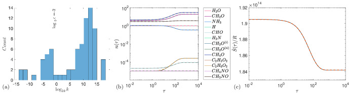
Figure 2: The slow dynamics equation can be applied to CRNs with a broad range of reaction rates. In (a) the histogram of reaction rates is shown (including both forward and reverse reactions), along with the chosen value of $\epsilon$ in simulations. Numerical integration of the rate equations (b, colors) is shown along with the prediction from slow dynamics (b, black). The entropy production (c, colors) is well predicted by the slow dynamics contribution (c, black).

In realistic CRNs at room temperature, the reaction rates span a wide range of scales. This presents challenges both for numerical simulations and for the basis of our theory, which requires a time-scale separation between the bulk and the reservoir interactions. Nevertheless, at high enough temperature such a separation can be found and the theory applied. Here we consider an ‘early Earth’ CRN modelling a submarine hydrothermal system containing formaldehyde, ammonia, and water, of interest for the origin of life as submarine hydrothermal systems are a potential source of abiotic amino acids Martin08 ; Smith16 . Using Reaction Mechanism Generator (see Methods) we obtain species that can be obtained from the initial pool, along with the corresponding reactions, including their rates; the full list of 13 species and 40 reactions is in SI.

This CRN conserves the concentrations of C, H, O, and N, so its slow dynamics is governed by only 4 DOF, a large reduction from the initial 13 DOF.

We solved the rate equations with reservoirs of $\mathrm{CH_{2}O,H,CH_{4}O}$, and $\mathrm{C_{2}H_{6}O_{2}}$ at T=1000K. For this choice of reservoirs, N is still conserved, as is the difference of C and O concentrations (since all reservoirs have an equal number of C and O atoms). Thus only 2 nontrivial DOF are needed to understand its slow dynamics. As shown in Figure 2, despite the range of reaction rates spanning 30 orders of magnitude and initial concentrations spanning more than 5 orders of magnitude, the slow dynamics equation quantitatively predicts the evolution of all species, and the entropy production.

V.4 Exponential growth

The slow dynamics equation is not limited to description of transients between equilibrium states; the theory also applies when a steady state is not reached. With the early Earth CRN, if coupled to reservoirs of $\mathrm{CH_{2}O,NH_{3},H,CHO,H_{2}N}$, then the system grows on the slow time scale $\tau$, as shown in SI. Again the slow dynamics equation captures this behavior.

V.5 Autotrophic Core

As a final example, we consider a very large reaction network of 404 reactions and 375 species, proposed in Wimmer21 as a minimal CRN from which to construct the amino acids and nucleic acid monomers necessary for life, along with cofactors needed for their synthesis, from primitive building blocks, namely H₂, CO₂, and NH₃; the authors have in mind an aqueous environment like a serpentizing hydrothermal vent Smith16 . Here we show how our theory can be used with such a CRN. More details on the CRN appear in SI.

On general grounds, whenever a reservoir is added to a CRN, then one of two things can happen: either a conservation law is broken, or a redundancy is created among the reservoirs, corresponding to an effective reaction performed by the CRN, also known as an emergent cycle; these can be obtained algebraically from the stoichiometric matrix Polettini14 ; Rao16 ; Wachtel22 . Existence of an emergent cycle is a necessary condition for a CRN to reach a non-equilibrium steady state. Moreover, many biologically important NESS have only a few emergent cycles Wachtel22 .

Consider first reservoirs of H₂O, H₂, CO₂, and NH₃, as suggested in Wimmer21 . These reservoirs break conservation of H, O, N, and C, and do not create any emergent cycles. Therefore the system cannot evolve to a NESS, but it can grow indefinitely, as indeed occurs. The slow dynamics is 4 dimensional, and easily solved numerically. Since the left-hand-side of the slow dynamics equation involves the $M$ matrix, which has contributions from the equilibrium concentrations of all species, then one needs to know the chemical potentials of all bulk species.

Consider now a scenario with more reservoirs. A minimal way to create a NESS is to add one emergent cycle. For example, if we add carbon monoxide $\ch{CO}$ then we create one emergent cycle

$$\ch{CO2}+\ch{H2} \xrightleftharpoons{}\ch{CO}+\ch{H2O}$$ (46)

Then when coupled to these reservoirs, the CRN can either grow indefinitely or evolve to a NESS, performing some of the effective reactions. NESS can be sought by looking for steady states of the slow dynamics. In terms of the net fluxes into the system from the reservoirs $J_{i}=r_{i}(z_{i}^{\mathscr{C}}-n_{i}^{0}/\Omega)$ these are

$$0 =J_{CO_{2}}+J_{CO}$$ (47)

$$0 =2J_{H_{2}O}+2J_{H_{2}}+3J_{NH_{3}}$$ (48)

$$0 =2J_{CO_{2}}+J_{CO}+J_{H_{2}O}$$ (49)

$$0 =J_{NH_{3}}$$ (50)

for C, H, O, and N, respectively. The last equation means that the system must equilibrate to be at the reservoir concentration of methane. Explicitly

$$0=r_{NH_{3}}(z_{NH_{3}}^{\mathscr{C}}-n_{NH_{3}}^{eq}e^{\eta_{N}}e^{3\eta_{H}}/\Omega)$$

implies $e^{\eta_{N}}=e^{-3\eta_{H}}z_{NH_{3}}^{\mathscr{C}}\Omega/n_{NH_{3}}^{eq}$. Note that $e^{\eta_{N}}$ depends on $e^{\eta_{H}}$, so it is still nontrivial – but since $J_{NH_{3}}=0$, it drops out of the remaining equations for the NESS.

To solve the remaining equations it is convenient to absorb equilibrium concentrations into the rates and reservoir concentrations, viz.,

$$J_{i}=r_{i}(z_{i}^{\mathscr{C}}-n_{i}^{eq}e^{\sum_{e}\zeta_{ie}\eta_{e}}/\Omega)\equiv\tilde{r}_{i}(\tilde{z}_{i}-e^{\sum_{e}\zeta_{ie}\eta_{e}})$$ (51)

Then labelling the reservoirs in the order $(\ch{H2O},\ch{H2},\ch{CO2},\ch{NH3},\ch{CO})$ the remaining equations reduce to

$$0 =\tilde{r}_{3}(\tilde{z}_{3}-e^{\eta_{C}+2\eta_{O}})+\tilde{r}_{5}(\tilde{z}_{5}-e^{\eta_{C}+\eta_{O}})$$ (52)

$$0 =\tilde{r}_{1}(\tilde{z}_{1}-e^{2\eta_{H}+\eta_{O}})+\tilde{r}_{2}(\tilde{z}_{2}-e^{2\eta_{H}})$$ (53)

$$0 =\tilde{r}_{3}(\tilde{z}_{3}-e^{\eta_{C}+2\eta_{O}})+\tilde{r}_{1}(\tilde{z}_{1}-e^{2\eta_{H}+\eta_{O}})$$ (54)

Solving the first two

$$e^{\eta_{C}} =e^{-\eta_{O}}\frac{\tilde{r}_{3}\tilde{z}_{3}+\tilde{r}_{5}\tilde{z}_{5}}{\tilde{r}_{3}e^{\eta_{O}}+\tilde{r}_{5}}$$ (55)

$$e^{2\eta_{H}} =\frac{\tilde{r}_{1}\tilde{z}_{1}+\tilde{r}_{2}\tilde{z}_{2}}{\tilde{r}_{1}e^{\eta_{O}}+\tilde{r}_{2}}$$ (56)

we reduce the problem to

$$0 =\tilde{r}_{3}\tilde{z}_{3}+\tilde{r}_{1}\tilde{z}_{1}-\tilde{r}_{3}\frac{\tilde{r}_{3}\tilde{z}_{3}+\tilde{r}_{5}\tilde{z}_{5}}{\tilde{r}_{3}e^{\eta_{O}}+\tilde{r}_{5}}e^{\eta_{O}}-\tilde{r}_{1}\frac{\tilde{r}_{1}\tilde{z}_{1}+\tilde{r}_{2}\tilde{z}_{2}}{\tilde{r}_{1}e^{\eta_{O}}+\tilde{r}_{2}}e^{\eta_{O}},$$ (57)

which becomes a quadratic equation for $e^{\eta_{O}}$. Thus NESS can easily be found. Now, for given reservoir rates and concentrations, one must check that each $e^{\eta_{e}}$ is positive; otherwise the solution is not physical.

Physical solutions can further be divided into two classes: if all the $\eta_{e}$ are negative, then the equilibrium concentrations of molecules at infinite temperature decrease with increasing atomic number: larger molecules are less abundant. Instead if some $\eta_{e}>0$, then that element leads to an increasing concentration with increasing atomic number: large molecules can become exponentially more abundant in the NESS. This opens the possibility for a phase transition separating such regimes, which can be probed with the slow dynamics equation, with further subtleties at finite $T$ depending on the behavior of chemical potentials with atomic composition. We leave the detailed study of this effect to the future. Here, we simply solved (57) for a variety of reservoir rates and concentrations, found solutions with all $\eta_{e}<0$, and then compared the result with that of the full rate equations. They agree, showing that the general structure of potential NESS can be probed without knowledge of the CRN bulk, even for very large CRNs, in the slow driving limit.

For this CRN, we also looked at examples with numerous reservoirs. In such cases, without fine-tuning of parameters, one finds that the system grows; this behavior was then confirmed by solution of the full rate equations. Examples are shown in SI.

VI Extension to far-from-equilibrium states

Although above we considered initial states that were near equilibrium before coupling to external reservoirs, this is not essential to obtain a reduction to conserved quantities. Suppose instead that there is a leading order coupling to reservoirs, which we assume is stationary. Write $\vec{r}\to\mbox{$\frac{1}{\epsilon}$}\vec{r}^{0}+\vec{r}$ so that the rate equation, in the two-time ansatz, is

$$\partial_{t}{\vec{n}}+\epsilon\partial_{\tau}{\vec{n}}=\underbrace{(\mathbb{S}^{0})\cdot{\vec{J}}^{\;0}({\vec{n}})+[\vec{r}^{0}({\vec{n}}^{\mathscr{C}}-{\vec{n}})]}_{\tilde{\mathbb{S}}\cdot\tilde{\vec{J}}^{\;0}({\vec{n}})}+\epsilon[\vec{r}({\vec{n}}^{\mathscr{C}}-{\vec{n}})]$$

Expanding ${\vec{n}}={\vec{n}}^{0}+\epsilon{\vec{n}}^{1}+\ldots$, at leading order $\partial_{t}{\vec{n}}^{0}=\tilde{\mathbb{S}}\cdot\tilde{\vec{J}}^{\;0}({\vec{n}}^{0})$. With time-independent coupling to reservoirs, this will either describe relaxation to a non-equilibrium steady state (NESS), or blow-up. Assume that we reach a NESS. Then at the next order we have an equation of the form (III), with $\mathbb{S}$ replaced by $\tilde{\mathbb{S}}$. This will generally have long-time divergences unless ${\vec{n}}^{0}$ depends on the slow time $\tau$. Let $\zeta$ be a basis of the conserved quantities of $\tilde{\mathbb{S}}$, i.e. $\tilde{\mathbb{S}}^{T}\cdot\zeta=0$. Then the slow dynamics equation is again (23). The differences with the previous analysis are that now (i) the conserved quantities do not necessarily correspond to elements, since the leading-order reservoirs will break some conservation laws; and (ii) ${\vec{n}}^{0}$ is not a known function of the slow DOF ${\vec{\eta}}$. This latter fact means that although true, (23) cannot be solved without constitutive information on the ${\vec{n}}^{0}({\vec{\eta}})$ relationship. Moreover, this unknown relationship ${\vec{n}}^{0}({\vec{\eta}})$ will in general involve the bulk reaction rates, unlike the detailed-balanced case. The main result here is that one knows the dimension of the reduced dynamics, equal to the number of conserved quantities of the NESS.

VII Discussion & Conclusions

We have shown that slowly driven CRNs are governed by the conserved quantities of the corresponding closed system. The latter are generally the element concentrations, giving a huge reduction in DOF in large CRNs. The natural dynamical variables of the slow dynamics are chemical potentials, ${\vec{\eta}}$, which evolve according to (25). From the solution of this equation, which does not involve the bulk reaction rates, one can obtain the full dynamics, at leading order in driving. Moreover, in this limit one can easily probe the structure of NESS for large, realistic CRNs.

This framework may be useful to understand free energy transduction in open CRNs Wachtel22 . Indeed, open CRNs can be considered as chemical machines that interconvert species between the reservoirs. For example, the early Earth CRN considered above, when coupled to reservoirs of $\mathrm{CH_{2}O,H,CH_{4}O}$, and $\mathrm{C_{2}H_{6}O_{2}}$, has effective reactions (emergent cycles)

$$\ch{CH_{2}O}+2\ch{H} \xrightleftharpoons{}\ch{CH_{4}O}$$ (58)

$$\ch{CH_{2}O}+\ch{CH_{4}O} \xrightleftharpoons{}\ch{C_{2}H_{6}O_{2}}.$$ (59)

The free energy change in an emergent cycle is obtained straightforwardly from the chemical potentials of the species, but to understand the efficiency of the chemical machine, one requires the flux through the cycle, except in special cases Wachtel22 . Generally this necessitates the entire suite of reaction rates and a numerical solution of the rate equations. A limiting factor in the analysis is then that many rates are not known for biochemical networks of interest.

Our analysis provides an alternative. For any given forcing, one can solve the slow dynamics equation, without knowledge of any bulk reaction rates. With this solution in hand, one can evaluate the reaction fluxes and then the efficiency. This solution is guaranteed to work in the limit of slow driving, and can provide a benchmark value at finite-rate driving.

For similar reasons, our theory may be useful in conjunction with a circuit theory for CRNs Avanzini23 . In the latter, a CRN is coarse-grained by treating subsets of CRNs as chemical modules, connected to each other by particular species. For each module, the theory requires the relationship between the flux through emergent cycles and the concentrations of chemostatted species. If a module is treated as fast compared to its external connections, then our theory can be used to find the current-concentration relations, as shown in SI for an example from Avanzini23 . This is particularly useful for large, poorly-characterized modules where our method does not require the bulk reaction rates.

Independence of the slow dynamics with respect to bulk activation energies is a strong, generic form of robustness applicable to all chemical machines whose core is detailed-balanced. Moreover, dissipation is minimized, since the system is always close to some equilibrium state. The price of this robustness is that the system responds slowly to outside forcing. Whether this slow dynamics is relevant for real-world chemical machines then depends on system-specific tradeoffs between robustness and speed.

We note that an alternative weak-driving theory has been obtained in Freitas21 , also using the Hamilton-Jacobi equation. This theory is based upon the log-probability correction $\rho_{1}$, but without the multiple time scale analysis. This is sufficient for non-equilibrium steady states as considered in Freitas21 , but in dynamical problems it will generally suffer from long-time divergences.

Our reduction of complex dynamics to that of the conserved quantities is reminiscent of hydrodynamics. There are, however, some differences. First, in hydrodynamics one assumes that the system is coupled to other systems that differ only weakly from it. Here instead we do not assume that the reservoirs are near the system: their concentrations can be arbitrarily far from the corresponding concentration in the system. We only assume that they react slowly with the system. Second, in hydrodynamics one considers systems that interact spatially, whereas our system is well-mixed and interacts with external reservoirs without any explicit spatial coupling. The extension of our results to include spatial effects will be presented in a future publication.

Methods:

For constructing the methane combustion model, the toolbox ”Stoichiometry Tools” in MATLAB was used Kantor23 . The input $\{\ch{CH4},\ch{CO2},\ch{H2O},\ch{CO},\ch{O2},\ch{H2}\}$ led to the reactions (40).

For larger models, we used Reaction Mechanism Generator (RMG) Gao16 ; Liu21 . Given an input pool of species, RMG iteratively finds possible reactions between the species and new species that can be produced. Rates, enthalpies, and entropies are either looked up in a database, or estimated using additivity methods. For the early Earth model, we used the input set $\{\ch{CH2O},\ch{NH3},\ch{H2O}\}$, with $\ch{H2O}$ as a solvent, into RMG. It results in the 40 reactions and 10 new species shown in SI.

We note that RMG is not guaranteed to find all possible reactions among species. In testing against known CRNs relevant to the origin of life, we found that RMG sometimes failed to find reactions known to be possible. Thus we use it as a method to benchmark our framework against CRNs with valid stoichiometry and a broad range of realistic rates.

For the autotrophic core CRN, we worked only at $T\to\infty$ so that no bulk reaction rates or chemical potentials were needed.

All ordinary differential equations were integrated in MATLAB using the ode15s solver.

References

- (1) Okino M S and Mavrovouniotis M L 1998 Chemical reviews 98 391–408
- (2) Radulescu O, Gorban A N, Zinovyev A and Noel V 2012 Frontiers in genetics 3 131
- (3) Snowden T J, van der Graaf P H and Tindall M J 2017 Bulletin of mathematical biology 79 1449–1486
- (4) Schneider K R and Wilhelm T 2000 Journal of mathematical biology 40 443–450
- (5) Bressloff P C 2017 Journal of Physics A: Mathematical and Theoretical 50 133001
- (6) Peng L and Hong L 2023 arXiv preprint arXiv:2308.06770
- (7) Chaikin P M and Lubensky T C 2000 Principles of Condensed Matter Physics (Cambridge, U.K.: Cambridge University Press) ISBN 9780521794503
- (8) Ren Z, Pope S B, Vladimirsky A and Guckenheimer J M 2006 The Journal of chemical physics 124
- (9) Lee C H and Othmer H G 2010 Journal of mathematical biology 60 387–450
- (10) Desoeuvres A, Iosif A, Lüders C, Radulescu O, Rahkooy H, Seiß M and Sturm T 2022 arXiv preprint arXiv:2212.13474
- (11) Schmiedl T and Seifert U 2007 The Journal of chemical physics 126 044101
- (12) Seifert U 2012 Reports on progress in physics 75 126001
- (13) Van den Broeck C 2013 Stochastic thermodynamics: A brief introduction vol 184 (IOS Press Amsterdam) pp 155–193
- (14) Wachtel A, Rao R and Esposito M 2018 New Journal of Physics 20 042002
- (15) Wachtel A, Rao R and Esposito M 2022 The Journal of Chemical Physics 157 024109
- (16) Avanzini F, Freitas N and Esposito M 2023 Physical Review X 13 021041
- (17) Polettini M and Esposito M 2014 The Journal of chemical physics 141 024117
- (18) Rao R and Esposito M 2016 Physical Review X 6 041064
- (19) Astumian R D 2018 Chemical Communications 54 427–444
- (20) Gilbert R G and Smith S C 1990 Theory of unimolecular and recombination reactions (Publishers’ Business Services [distributor])
- (21) Bender C M and Orszag S A 1999 Advanced Mathematical Methods for Scientists and Engineers vol I (Springer)
- (22) Hinch E J 1991 Matched Asymptotic Expansions 1st ed (Cambridge, U.K.: Cambridge)
- (23) De Martino A, Martelli C and Massucci F A 2009 EPL (Europhysics Letters) 85 38007
- (24) Doi M 1976 Journal of Physics A: Mathematical and General 9 1465
- (25) Peliti L 1985 Journal de Physique 46 1469–1483
- (26) De Giuli E and Scalliet C 2022 Journal of Physics A: Mathematical and Theoretical 55 474002
- (27) Kubo R, Matsuo K and Kitahara K 1973 Journal of Statistical Physics 9 51–96
- (28) Kitahara K 1975
- (29) Smith E 2020 Entropy 22 1137
- (30) Gillespie D T 1977 The journal of physical chemistry 81 2340–2361
- (31) Martin W, Baross J, Kelley D and Russell M J 2008 Nature Reviews Microbiology 6 805–814 URL https://doi.org/10.1038/nrmicro1991
- (32) Smith E and Morowitz H J 2016 The origin and nature of life on earth: the emergence of the fourth geosphere (Cambridge University Press)
- (33) Wimmer J L, Vieira A d N, Xavier J C, Kleinermanns K, Martin W F and Preiner M 2021 Microorganisms 9 458
- (34) Freitas N, Falasco G and Esposito M 2021 New Journal of Physics 23 093003
- (35) Kantor J 2023 Stoichiometry tools URL https://www.mathworks.com/matlabcentral/fileexchange/29774-stoichiometry-tools
- (36) Gao C W, Allen J W, Green W H and West R H 2016 Computer Physics Communications 203 212–225
- (37) Liu M, Grinberg Dana A, Johnson M S, Goldman M J, Jocher A, Payne A M, Grambow C A, Han K, Yee N W and Mazeau E J 2021 Journal of Chemical Information and Modeling 61 2686–2696