Holography in anomaly flow in orbifold gauge theory

Abstract

In orbifold gauge theory and gauge-Higgs unification models, gauge anomaly flows with an Aharonov-Bohm phase $\theta_{H}$ in the fifth dimension. We analyze $SU(2)$ gauge theory with doublet fermions in the flat $M^{4}\times(S^{1}/Z_{2})$ spacetime and in the Randall-Sundrum (RS) warped space. With orbifold boundary conditions the $U(1)$ part of gauge symmetry remains unbroken at $\theta_{H}=0$ and $\pi$. Chiral anomalies smoothly vary with $\theta_{H}$ in the RS space. Anomaly coefficients associated with this anomaly flow are expressed in terms of the values of the wave functions of gauge fields at the UV and IR branes in the RS space and parity conditions of fermion fields. Holography in anomaly flow is observed. Conditions for the anomaly cancellation turn out independent of $\theta_{H}$.

1 Introduction

Chiral fermions generally induce chiral anomaly.[1, 2, 3] Even for massive fermions chiral anomaly can be generated if gauge couplings are not purely vector-like. Something special happens in gauge-Higgs unification (GHU), in which gauge symmetry is dynamically broken by an Aharonov-Bohm (AB) phase $\theta_{H}$ in the fifth dimension.[4, 5, 6] It has been noticed in the GUT inspired $SO(5)\times U(1)_{X}\times SU(3)_{C}$ GHU in the Randall-Sundrum (RS) warped space [7] that quarks and leptons are massless and purely chiral at $\theta_{H}=0$, become massive at $\theta_{H}\not=0$, and smoothly become vector-like at $\theta_{H}=\pi$. Gauge bosons such as $W$ and $Z$ bosons are massless gauge bosons of $SU(2)_{L}\times U(1)_{Y}$ at $\theta_{H}=0$, become massive at $\theta_{H}\not=0$, and smoothly converted to massless gauge bosons of $SU(2)_{R}\times U(1)_{Y^{\prime}}$ at $\theta_{H}=\pi$. This prompts the following question. What happens to the anomaly generated by chiral quarks and leptons at $\theta_{H}=0$? Does it disappear at $\theta_{H}=\pi$? What is the fate of chiral anomaly?

To pin down what is going on in GHU formulated on orbifolds, the dependence of chiral anomaly on the AB phase $\theta_{H}$ in $SU(2)$ gauge theory with doublet fermions in the flat $M^{4}\times(S^{1}/Z_{2})$ space and in the RS warped space has been investigated in Refs. [8, 9]. In the flat $M^{4}\times(S^{1}/Z_{2})$ space the mass spectrum of the Kaluza-Klein (KK) modes of gauge bosons and fermions changes linearly in $\theta_{H}$, namely as $m_{n}=|n+(\theta_{H}/\pi)|/R$ or $|n+(\theta_{H}/2\pi)|/R$, so that the level crossing takes place where $\theta_{H}$ is a multiple of $\hbox{$\frac{1}{2}$}\pi$ or $\pi$. In the RS space there occurs no level crossing in the mass spectrum. The spectrum varies smoothly as $\theta_{H}$ changes from 0 to $2\pi$. The lowest mode remains as the lowest mode for any $\theta_{H}$. Gauge couplings of right- and left-handed modes of fermions vary smoothly as $\theta_{H}$, and the magnitude of chiral anomaly also changes as $\theta_{H}$. The anomaly coefficient (defined below) coming from one doublet fermion changes from $2$ at $\theta_{H}=0$ to $0$ at $\theta_{H}=\pi$. The anomaly flows with the AB phase $\theta_{H}$.

Furthermore it was shown that the magnitude of the total anomaly evaluated by summing contributions coming from all KK modes of fermions running along internal loops is expressed in terms of the values of the wave functions of the gauge fields at the two branes (the UV and IR branes in the RS space) and the parity conditions of fermion fields at the two branes. Each fermion field in the RS space is characterized by its own bulk mass parameter $c$ which controls its mass and wave function at general $\theta_{H}$. Although the anomaly coming from each KK mode depends on the bulk mass parameter $c$, the total anomaly does not depend on $c$. There emerges a holographic formula for the total anomaly. This holography becomes crucial to have the cancellation of gauge anomalies in GHU.

2 $SU(2)$ GHU in $M^{4}\times(S^{1}/Z_{2})$

Let us first consider $SU(2)$ GHU in the flat $M^{4}\times(S^{1}/Z_{2})$ spacetime with coordinate $x^{M}$ ($M=0,1,2,3,5$, $x^{5}=y$) whose action is given by

$$I_{\rm flat} =\int d^{4}x\int_{0}^{L}dy\,{\cal L}_{\rm flat}~{},~{}~{}{\cal L}_{\rm flat}=-\frac{1}{2}{\rm Tr}\,F_{MN}F^{MN}+\overline{\Psi}\gamma^{M}(\partial_{M}-ig_{A}A_{M})\Psi~{},$$ (2.1)

where ${\cal L}_{\rm flat}(x^{\mu},y)={\cal L}_{\rm flat}(x^{\mu},y+2L)={\cal L}_{\rm flat}(x^{\mu},-y)$. $A_{M}=\hbox{$\frac{1}{2}$}\sum_{a=1}^{3}A^{a}_{M}\tau^{a}$ and $F_{MN}=\partial_{M}A_{N}-\partial_{N}A_{N}-ig_{A}[A_{M},A_{N}]$ where $\tau^{a}$’s are Pauli matrices. Orbifold boundary conditions are given, with $(y_{0},y_{1})=(0,L)$ and $P_{0}=P_{1}=\tau^{3}$, by

$$\begin{pmatrix}A_{\mu}\cr A_{y}\end{pmatrix}(x,y_{j}-y)=P_{j}\begin{pmatrix}A_{\mu}\cr-A_{y}\end{pmatrix}(x,y_{j}+y)P_{j}^{-1}~{},$$ (2.2)

$$\Psi(x,y_{j}-y)=\begin{cases}+P_{j}\gamma^{5}\Psi(x,y_{j}+y)&\hbox{type 1A}\cr\kern 1.0pt\cr-P_{j}\gamma^{5}\Psi(x,y_{j}+y)&\hbox{type 1B}\cr\kern 1.0pt\cr(-1)^{j}P_{j}\gamma^{5}\Psi(x,y_{j}+y)&\hbox{type 2A}\cr\kern 1.0pt\cr(-1)^{j+1}P_{j}\gamma^{5}\Psi(x,y_{j}+y)&\hbox{type 2B}\end{cases}~{}.$$ (2.3)

The $SU(2)$ symmetry is broken to $U(1)$. $A^{3}_{\mu}$ and $A^{1,2}_{y}$ are parity even at both $y_{0}$ and $y_{1}$. The zero mode of $A^{3}_{\mu}$ is the 4D $U(1)$ gauge field. The 4D gauge coupling is given by $g_{4}=g_{A}/\sqrt{L}$. The zero modes of $A_{y}^{1,2}$ may develop nonvanishing expectation values. Without loss of generality we assume $\langle A_{y}^{1}\rangle=0$. An AB phase $\theta_{H}$ along the fifth dimension is then given by

$$P\exp\bigg{\{}ig_{A}\int_{0}^{2L}dy\,\langle A_{y}\rangle\bigg{\}}=e^{i\theta_{H}\tau^{2}}~{},~{}~{}\theta_{H}=g_{4}L\,\langle A_{y}^{2}\rangle~{}.$$ (2.4)

When $\theta_{H}\not=0$, $A_{\mu}^{1}$ and $A_{\mu}^{3}$ intertwine with each other. It is straightforward to find mass eigenstates. The KK expansion is given by

$$\begin{pmatrix}A_{\mu}^{1}(x,y)\cr\kern 2.0pt\cr A_{\mu}^{3}(x,y)\end{pmatrix} =\sum_{n=-\infty}^{\infty}B_{\mu}^{(n)}(x)\frac{1}{\sqrt{\pi R}}\begin{pmatrix}\sin(ny/R)\cr\cos(ny/R)\end{pmatrix}$$ (2.5)

where $R=L/\pi$. The mass of the $B_{\mu}^{(n)}(x)$ mode is $m_{n}(\theta_{H})=R^{-1}\big{|}n+\frac{\theta_{H}}{\pi}\big{|}$. The spectrum is periodic in $\theta_{H}$ with a period $\pi$. The KK expansion of a doublet fermion $\Psi=(u,d)^{t}$ of type 1A is given by

$$\begin{pmatrix}u_{R}(x,y)\cr\kern 2.0pt\cr d_{R}(x,y)\end{pmatrix} =\sum_{n=-\infty}^{\infty}\psi_{R}^{(n)}(x)\frac{1}{\sqrt{\pi R}}\begin{pmatrix}\cos(ny/R)\cr\sin(ny/R)\end{pmatrix},$$ (2.6)

$$\begin{pmatrix}u_{L}(x,y)\cr\kern 2.0pt\cr d_{L}(x,y)\end{pmatrix} =\sum_{n=-\infty}^{\infty}\psi_{L}^{(n)}(x)\frac{1}{\sqrt{\pi R}}\begin{pmatrix}-\sin(ny/R)\cr\cos(ny/R)\end{pmatrix}.$$ (2.7)

$\psi_{R}^{(n)}$ and $\psi_{L}^{(n)}$ combine to form the $\psi^{(n)}(x)$ mode with a mass given by $m_{n}(\theta_{H})=R^{-1}\big{|}n+\frac{\theta_{H}}{2\pi}\big{|}$. The spectrum is periodic in $\theta_{H}$ with a period $2\pi$. Note that the KK mass scale in the flat space is $m_{\rm KK}^{\rm flat}=1/R$.

3 $SU(2)$ GHU in the Randall-Sundrum warped space

The metric of the RS warped space is given by [10]

$$ds^{2}=e^{-2\sigma(y)}\eta_{\mu\nu}dx^{\mu}dx^{\nu}+dy^{2}$$ (3.1)

where $\eta_{\mu\nu}=\mbox{diag}(-1,+1,+1,+1)$, $\sigma(y)=\sigma(y+2L)=\sigma(-y)$ and $\sigma(y)=ky$ for $0\leq y\leq L$. It has the same topology as $M^{4}\times(S^{1}/Z_{2})$. In the region $0\leq y\leq L$ the metric can be written, in terms of the conformal coordinate $z=e^{ky}$, as

$$ds^{2}=\frac{1}{z^{2}}\bigg{(}\eta_{\mu\nu}dx^{\mu}dx^{\nu}+\frac{dz^{2}}{k^{2}}\bigg{)}\quad(1\leq z\leq z_{L}=e^{kL})~{}.$$ (3.2)

$z_{L}$ is called the warp factor of the RS space. The RS space is an anti-de Sitter (AdS) space sandwiched by the UV brane at $y=0~{}(z=1)$ and the IR brane at $y=L~{}(z=z_{L})$. The AdS curvature is given by $\Lambda=-6k^{2}$.

The action in the RS space is given by

$$I_{\rm RS}=\int d^{5}x\sqrt{-\det G}\,{\cal L}_{\rm RS}~{},~{}~{}{\cal L}_{\rm RS}=-\frac{1}{2}{\rm Tr}\,F_{MN}F^{MN}+\overline{\Psi}{\cal D}(c)\Psi~{},$$ (3.3)

$${\cal D}(c)=\gamma^{A}{e_{A}}^{M}\Big{(}\partial_{M}-ig_{A}A_{M}+\frac{1}{8}\omega_{MBC}[\gamma^{B},\gamma^{C}]\Big{)}-c\,\sigma^{\prime}~{}.$$ (3.4)

$c$ is a dimensionless bulk mass parameter. Note ${\cal L}_{\rm RS}(x^{\mu},y)={\cal L}_{\rm RS}(x^{\mu},-y)={\cal L}_{\rm RS}(x^{\mu},y+2L)$. Fields $A_{M}$ and $\Psi$ satisfy the same boundary conditions (2.3) as in the flat spacetime. The AB phase $\theta_{H}$ and the KK mass scale $m_{\rm KK}$ are given by

$$\theta_{H} =\frac{\langle A_{z}^{2(0)}\rangle}{f_{H}}~{},~{}~{}f_{H}=\frac{1}{g_{4}}\sqrt{\frac{2k}{L(z_{L}^{2}-1)}}~{},~{}~{}m_{\rm KK}=\frac{\pi k}{z_{L}-1}~{},$$ (3.5)

where $A_{z}^{a}(x,z)=k^{-1/2}\sum A_{z}^{a(n)}(x)v_{n}(z)$ and $v_{0}(z)=\sqrt{2/(z_{L}^{2}-1)}\,z$.

The KK expansion of the gauge fields $A_{\mu}^{1}$ and $A_{\mu}^{3}$ is given by

$$\begin{pmatrix}A_{\mu}^{1}(x,y)\cr\kern 1.0pt\cr A_{\mu}^{3}(x,y)\end{pmatrix}=\frac{1}{\sqrt{L}}\sum_{n=0}^{\infty}Z_{\mu}^{(n)}(x)\,\begin{pmatrix}h_{n}(y)\cr k_{n}(y)\end{pmatrix},$$ (3.6)

$$\begin{pmatrix}h_{n}(y)\cr k_{n}(y)\end{pmatrix}=\begin{pmatrix}-h_{n}(-y)\cr k_{n}(-y)\end{pmatrix}=\begin{pmatrix}h_{n}(y+2L)\cr k_{n}(y+2L)\end{pmatrix}$$ (3.7)

$$=\begin{pmatrix}\cos\theta(z)&\sin\theta(z)\cr-\sin\theta(z)&\cos\theta(z)\end{pmatrix}\begin{pmatrix}\tilde{h}_{n}(z)\cr\tilde{k}_{n}(z)\end{pmatrix},~{}~{}\theta(z)=\theta_{H}\,\frac{z_{L}^{2}-z^{2}}{z_{L}^{2}-1}\quad{\rm for~{}}0\leq y\leq L~{}.$$ (3.8)

The mass spectrum $\{m_{n}=k\lambda_{n};~{}\lambda_{0}<\lambda_{1}<\lambda_{2}<\cdots\}$ of the KK modes $\big{\{}Z_{\mu}^{(n)}(x)\big{\}}$ is determined by the zeros of

$$Z_{\mu}^{(n)}:~{}SC^{\prime}(1;\lambda_{n})+\lambda_{n}\sin^{2}\theta_{H}=0$$ (3.9)

where $S(z;\lambda)$ and $C(z;\lambda)$ are expressed in terms of Bessel functions and are given by (A.5). The wave functions $\tilde{\bf h}_{n}(z)\equiv(\tilde{h}_{n}(z),\tilde{k}_{n}(z))^{t}$ are given by (B.6).

For fermion fields we define $\check{\Psi}(x,z)=z^{-2}\,\Psi(x,z)$ for $1\leq z\leq z_{L}$. The KK expansion of $\check{\Psi}=(\check{u},\check{d})^{t}$ of type 1A is given by

$$\begin{pmatrix}{\check{u}}_{R}(x,y)\cr\kern 2.0pt\cr{\check{d}}_{R}(x,y)\end{pmatrix} =\sqrt{k}\sum_{n=0}^{\infty}\chi_{R}^{(n)}(x)\begin{pmatrix}f_{Rn}(y)\cr g_{Rn}(y)\end{pmatrix},$$ (3.10)

$$\begin{pmatrix}{\check{u}}_{L}(x,y)\cr\kern 2.0pt\cr{\check{d}}_{L}(x,y)\end{pmatrix} =\sqrt{k}\sum_{n=0}^{\infty}\chi_{L}^{(n)}(x)\begin{pmatrix}f_{Ln}(y)\cr g_{Ln}(y)\end{pmatrix},$$ (3.11)

where

$$\begin{pmatrix}f_{Rn}(y)\cr g_{Rn}(y)\end{pmatrix}=\begin{pmatrix}f_{Rn}(-y)\cr-g_{Rn}(-y)\end{pmatrix}=\begin{pmatrix}f_{Rn}(y+2L)\cr g_{Rn}(y+2L)\end{pmatrix}$$ (3.12)

$$\quad=\begin{pmatrix}\cos\hbox{$\frac{1}{2}$}\theta(z)&-\sin\hbox{$\frac{1}{2}$}\theta(z)\cr\kern 1.0pt\cr\sin\hbox{$\frac{1}{2}$}\theta(z)&\cos\hbox{$\frac{1}{2}$}\theta(z)\end{pmatrix}\begin{pmatrix}\tilde{f}_{Rn}(z)\cr\tilde{g}_{Rn}(z)\end{pmatrix}\quad{\rm for~{}}0\leq y\leq L~{},$$ (3.13)

$$\begin{pmatrix}f_{Ln}(y)\cr g_{Ln}(y)\end{pmatrix}=\begin{pmatrix}-f_{Ln}(-y)\cr g_{Ln}(-y)\end{pmatrix}=\begin{pmatrix}f_{Ln}(y+2L)\cr g_{Ln}(y+2L)\end{pmatrix}$$ (3.14)

$$\quad=\begin{pmatrix}\cos\hbox{$\frac{1}{2}$}\theta(z)&-\sin\hbox{$\frac{1}{2}$}\theta(z)\cr\kern 1.0pt\cr\sin\hbox{$\frac{1}{2}$}\theta(z)&\cos\hbox{$\frac{1}{2}$}\theta(z)\end{pmatrix}\begin{pmatrix}\tilde{f}_{Ln}(z)\cr\tilde{g}_{Ln}(z)\end{pmatrix}\quad{\rm for~{}}0\leq y\leq L~{}.$$ (3.15)

$\chi_{R}^{(n)}(x)$ and $\chi_{L}^{(n)}(x)$ combine to form a massive mode $\chi^{(n)}(x)$ for $\theta_{H}\not=0$. The mass spectrum $\{m_{n}=k\lambda_{n};~{}\lambda_{0}<\lambda_{1}<\lambda_{2}<\cdots\}$ of the KK modes $\{\chi^{(n)}(x)\}$ is determined by the zeros of

$$\chi^{(n)}:~{}S_{L}S_{R}(1;\lambda_{n},c)+\sin^{2}\hbox{$\frac{1}{2}$}\theta_{H}=0$$ (3.16)

where $S_{L}(z;\lambda,c)$ and $S_{R}(z;\lambda,c)$ are given by (A.10). The wave functions $\tilde{\bf f}_{Rn}(z)=(\tilde{f}_{Rn}(z),\tilde{g}_{Rn}(z))^{t}$ and $\tilde{\bf f}_{Ln}(z)=(\tilde{f}_{Ln}(z),\tilde{g}_{Ln}(z))^{t}$ are given by (B.11).

The mass spectra as functions of $\theta_{H}$ in the flat $M^{4}\times(S^{1}/Z_{2})$ space and in the RS warped space are depicted in Fig. 1. In the flat space the mass spectrum of each field changes linearly in $\theta_{H}$ so that the level crossing occurs. In the RS space there is no level crossing so that physical quantities change smoothly as $\theta_{H}$. It is expected that in the flat space something singular may occur at $\theta_{H}=0,\hbox{$\frac{1}{2}$}\pi,\pi,\cdots$. This is exactly what is going to happen in the anomaly as is seen below.

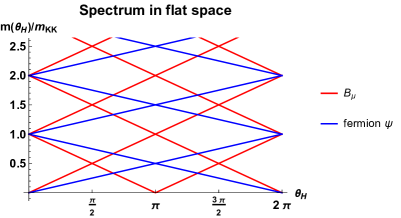
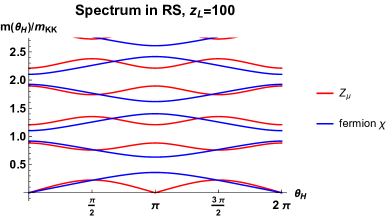
Figure 1: (Top): The mass spectrum of gauge fields $B_{\mu}^{(n)}$ and fermion fields $\psi^{(n)}$ (type 1A) in the flat $M^{4}\times(S^{1}/Z_{2})$ space is displayed. The level crossing occurs at $\theta_{H}=0,\hbox{$\frac{1}{2}$}\pi,\pi,\cdots$. (Bottom): The mass spectrum of gauge fields $Z_{\mu}^{(n)}$ and fermion fields $\chi^{(n)}$ (type 1A) in the RS warped space is displayed. The warp factor is $z_{L}=100$ and the bulk mass parameter of $\Psi$ is $c=0.25$.

4 Gauge couplings and anomaly in flat space

Gauge couplings of fermions in the flat space are easily found by inserting the KK expansions (2.5) and (2.7) into the action (2.1). One finds that the $B_{\mu}^{(n)}$ couplings of the fermion fields are given by

$$\sum_{n=-\infty}^{\infty}B_{\mu}^{\langle n\rangle}\,j^{\mu}_{(n)}$$ (4.1)

$$=\frac{g_{4}}{2}\sum_{n=-\infty}^{\infty}\sum_{m=-\infty}^{\infty}\sum_{\ell=-\infty}^{\infty}B_{\mu}^{\langle n\rangle}\Big{\{}s^{R}_{nm\ell}\,\psi_{R}^{\langle m\rangle\,\dagger}\bar{\sigma}^{\mu}\psi_{R}^{\langle\ell\rangle}+s^{L}_{nm\ell}\,\psi_{L}^{\langle m\rangle\,\dagger}\sigma^{\mu}\psi_{L}^{\langle\ell\rangle}\Big{\}}~{},$$ (4.2)

$$\hskip 85.35826pts^{R}_{nm\ell}=s^{L}_{nm\ell}=\delta_{n,m+\ell}~{}.$$ (4.3)

Here we have adopted the two-component notation; $\sigma^{\mu}=(I_{2},\vec{\sigma})$ and $\bar{\sigma}^{\mu}=(-I_{2},\vec{\sigma})$. Chiral anomaly in $\partial_{\mu}j^{\mu}_{(n)}$ arises from triangle diagrams in which various combinations of $\psi_{R/L}^{\langle\ell\rangle}$ run;

$$\partial_{\mu}j^{\mu}_{(n)}+\cdots=-\Big{(}\frac{g_{4}}{2}\Big{)}^{3}\sum_{\ell}\sum_{m}\frac{b_{n\ell m}}{16\pi^{2}}\,B_{\mu\nu}^{(\ell)}\tilde{B}^{(m)\mu\nu}$$ (4.4)

where $B_{\mu\nu}^{(\ell)}=\partial_{\mu}B_{\nu}^{(\ell)}-\partial_{\nu}B_{\mu}^{(\ell)}$. The anomaly coefficient $b_{n\ell m}$ is found to be

$$b_{n_{1}n_{2}n_{3}} =\sum_{m,\ell,p}\Big{\{}s_{n_{1}m\ell}^{R}s_{n_{2}\ell p}^{R}s_{n_{3}pm}^{R}+s_{n_{1}m\ell}^{L}s_{n_{2}\ell p}^{L}s_{n_{3}pm}^{L}\Big{\}}$$ (4.5)

$$=\begin{cases}2&{\rm for~{}}n_{1}+n_{2}+n_{3}={\rm even}\cr 0&{\rm for~{}}n_{1}+n_{2}+n_{3}={\rm odd}\end{cases}~{}.$$ (4.6)

Chiral anomalies arise even for $j^{\mu}_{(n\not=0)}$. A few examples are shown in Fig.  2.

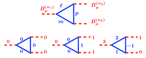
Figure 2: Chiral anomaly in the flat space.

5 Gauge couplings and anomaly in RS

Similarly gauge couplings of fermions in the RS space are expressed as

$$\sum_{n=0}^{\infty}Z_{\mu}^{\langle n\rangle}\,j^{\mu}_{(n)}$$ (5.1)

$$=\frac{g_{4}}{2}\sum_{n=0}^{\infty}\sum_{\ell=0}^{\infty}\sum_{m=0}^{\infty}Z_{\mu}^{(n)}\Big{\{}t^{R}_{n\ell m}\,\chi_{R}^{(\ell)\dagger}\bar{\sigma}^{\mu}\chi_{R}^{(m)}+t^{L}_{n\ell m}\,\chi_{L}^{(\ell)\dagger}\sigma^{\mu}\chi_{L}^{(m)}\Big{\}}~{}.$$ (5.2)

The couplings $t^{R}_{n\ell m}$ and $t^{L}_{n\ell m}$ are more involved. They are given, in terms of the wave functions in (3.8) and (3.15), by

$$t^{R}_{n\ell m}=\frac{k}{2}\int_{-L}^{L}dy\,e^{k|y|}\Big{\{}h_{n}\big{(}f_{R\ell}^{*}g_{Rm}+g_{R\ell}^{*}f_{Rm}\big{)}+k_{n}\big{(}f_{R\ell}^{*}f_{Rm}-g_{R\ell}^{*}g_{Rm}\big{)}\Big{\}},$$ (5.3)

$$t^{L}_{n\ell m}=-\frac{k}{2}\int_{-L}^{L}dy\,e^{k|y|}\Big{\{}h_{n}\big{(}f_{L\ell}^{*}g_{Lm}+g_{L\ell}^{*}f_{Lm}\big{)}+k_{n}\big{(}f_{L\ell}^{*}f_{Lm}-g_{L\ell}^{*}g_{Lm}\big{)}\Big{\}}.$$ (5.4)

Note that $t^{R/L}_{n\ell m}$ depends on $\theta_{H}$, $z_{L}$ and $c$. (It does not depend on $k$ or $m_{\rm KK}$.)

Chiral anomaly in $\partial_{\mu}j^{\mu}_{(n)}$ is written as

$$\partial_{\mu}j^{\mu}_{(n)}+\cdots=-\Big{(}\frac{g_{4}}{2}\Big{)}^{3}\sum_{\ell,m=0}^{\infty}\frac{a_{n\ell m}}{16\pi^{2}}\,Z_{\mu\nu}^{(\ell)}\tilde{Z}^{(m)\mu\nu}$$ (5.5)

where $Z_{\mu\nu}^{(\ell)}=\partial_{\mu}Z_{\nu}^{(\ell)}-\partial_{\nu}Z_{\mu}^{(\ell)}$. The anomaly coefficient $a_{n\ell m}$ is found to be

$$a_{n_{1}n_{2}n_{3}} =a_{n_{1}n_{2}n_{3}}^{R}+a_{n_{1}n_{2}n_{3}}^{L}~{},$$ (5.6)

$$a_{n_{1}n_{2}n_{3}}^{R/L} =\sum_{m,\ell,p=0}^{\infty}t_{n_{1}m\ell}^{R/L}\,t_{n_{2}\ell p}^{R/L}\,t_{n_{3}pm}^{R/L}~{}.$$ (5.7)

As the couplings $t^{R}_{n\ell m}$ and $t^{L}_{n\ell m}$ depend on $\theta_{H}$, $a^{R}_{n\ell m}$ and $a^{L}_{n\ell m}$ also do depend on $\theta_{H}$. In the RS space the dependence is smooth. For instance, $t^{R}_{000}$, $t^{L}_{000}$, $a^{R}_{000}$, $a^{L}_{000}$ and $a_{000}$ for $z_{L}=10$ and $c=0.25$ are depicted in Fig.  3. It is seen that $a_{000}$ changes from 2 to 0 as $\theta_{H}$ varies from 0 to $\pi$.

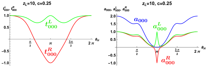
Figure 3: Gauge couplings $t^{R/L}_{000}$and anomaly coefficients $a^{R/L}_{000}$ and $a_{000}$ for $z_{L}=10$ and $c=0.25$ are shown as functions of $\theta_{H}$. $a^{R/L}_{000}$ and $a_{000}$ are evaluated by taking account of $t^{R/L}_{0m\ell}$ ($0\leq m,\ell\leq 14$).

6 Anomaly flow

In the flat space the anomaly coefficients $b_{nm\ell}$ in (4.6) are constant, whereas the anomaly coefficients $a_{nm\ell}$ in (5.7) in the RS space depend on $\theta_{H}$. There is no contradiction between these two facts. Look at the mass spectrum in Fig. 1. In the RS space the lowest mode of the gauge field is always $Z_{\mu}^{(0)}$ irrespective of the value of $\theta_{H}$. In the flat space the lowest mode is $B_{\mu}^{(0)}$ for $0<\theta_{H}<\hbox{$\frac{1}{2}$}\pi$, $B_{\mu}^{(-1)}$ for $\hbox{$\frac{1}{2}$}\pi<\theta_{H}<\frac{3}{2}\pi$, and $B_{\mu}^{(-2)}$ for $\frac{3}{2}\pi<\theta_{H}<2\pi$. The anomaly coefficient $b_{nnn}$ is $+2$ for $n=0$ and $-2$, but is 0 for $n=-1$. As the AdS curvature approaches 0, that is, as $k\rightarrow 0$, the RS space becomes the flat $M^{4}\times(S^{1}/Z_{2})$ space. In other words, $a_{000}$ must flow from 2 to 0 to 2 as $\theta_{H}$ changes from 0 to $\pi$ to $2\pi$. The anomaly flows as the AB phase $\theta_{H}$ varies. In the flat space the behavior of the anomaly becomes singular at the points of the level crossing, namely at $\theta_{H}=\hbox{$\frac{1}{2}$}\pi$ and $\frac{3}{2}\pi$.

The phenomenon of the anomaly flow is seen in all anomaly coefficients $a_{nm\ell}$. In Fig.  4 the anomaly coefficients $a^{R/L}_{012}$, $a_{012}$, $a^{R/L}_{222}$ and $a_{222}$ are plotted for $z_{L}=10$ and $c=0.25$. The anomaly flow is smooth.

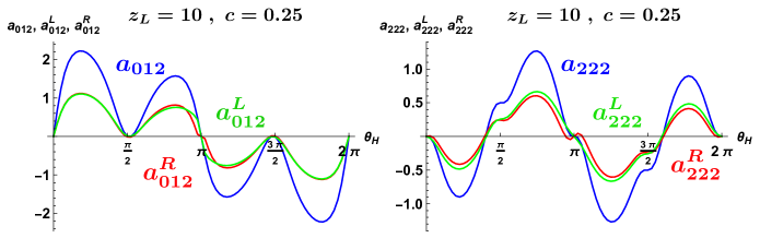
Figure 4: Anomaly coefficients $a^{R/L}_{012}$, $a_{012}$, $a^{R/L}_{222}$ and $a_{222}$ $a^{R/L}_{012}$, $a_{012}$, $a^{R/L}_{222}$ and $a_{222}$ for $z_{L}=10$ and $c=0.25$ are shown as functions of $\theta_{H}$. The coefficients are evaluated by taking account of $t^{R/L}_{jm\ell}$ ($j=0,1,2$, $0\leq m,\ell\leq 14$).

One might wonder how the anomaly flow in the RS space reduces to the anomaly flow in the flat space which seems singular at $\theta_{H}=\hbox{$\frac{1}{2}$}\pi$ and $\frac{3}{2}\pi$. The flat space limit is obtained by taking the $k\rightarrow 0$ limit in the RS space. As $k\rightarrow 0$ with $L=\pi R$ kept fixed, $z_{L}\rightarrow 1$. In Fig. 5 the behavior of $a_{000}(\theta_{H};z_{L})$ is shown.

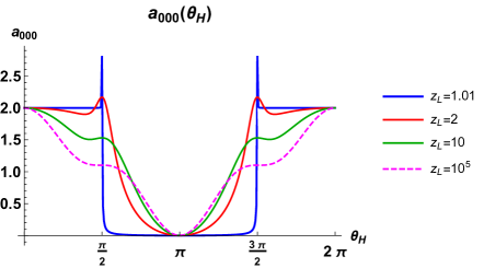
Figure 5: The $z_{L}$-dependence of the anomaly coefficient $a_{000}(\theta_{H};z_{L})$ is displayed for $c=0.25$.

One sees that $a_{000}(\theta_{H};z_{L})$ varies smoothly as $z_{L}$ changes. The $z_{L}\rightarrow 1$ limit is singular at $\theta_{H}=\hbox{$\frac{1}{2}$}\pi$ and $\frac{3}{2}\pi$, however.

$$\lim_{z_{L}\rightarrow 1}a_{000}(\theta_{H};z_{L})=\begin{cases}2&{\rm for~{}}0\leq\theta_{H}<\hbox{$\frac{1}{2}$}\pi\cr 2\sqrt{2}&{\rm for~{}}\theta_{H}=\hbox{$\frac{1}{2}$}\pi\cr 0&{\rm for~{}}\hbox{$\frac{1}{2}$}\pi\leq\theta_{H}<\frac{3}{2}\pi\cr 2\sqrt{2}&{\rm for~{}}\theta_{H}=\frac{3}{2}\pi\cr 2&{\rm for~{}}\frac{3}{2}\pi\leq\theta_{H}\leq 2\pi\end{cases}~{}.$$ (6.1)

This is precisely the behavior in the flat space as

$$\lim_{z_{L}\rightarrow 1}Z_{\mu}^{(0)}=\begin{cases}B_{\mu}^{(0)}&{\rm for~{}}0\leq\theta_{H}<\hbox{$\frac{1}{2}$}\pi\cr\frac{1}{\sqrt{2}}(B_{\mu}^{(0)}+B_{\mu}^{(-1)})&{\rm for~{}}\theta_{H}=\hbox{$\frac{1}{2}$}\pi\cr B_{\mu}^{(-1)}&{\rm for~{}}\hbox{$\frac{1}{2}$}\pi<\theta_{H}<\frac{3}{2}\pi\cr\frac{1}{\sqrt{2}}(B_{\mu}^{(-1)}+B_{\mu}^{(-2)})&{\rm for~{}}\theta_{H}=\frac{3}{2}\pi\cr B_{\mu}^{(-2)}&{\rm for~{}}\frac{3}{2}\pi<\theta_{H}\leq 2\pi\end{cases}~{}.$$ (6.2)

As a function of $\theta_{H}$, the anomaly coefficient $a_{000}(\theta_{H})$ becomes singular in the flat space limit at the points where level crossing occurs.

7 Holography in anomaly flow

In Figs. 3, 4 and 5, the anomaly coefficients coming from a fermion doublet of type 1A with the bulk mass parameter $c=0.25$ have been shown. A surprise comes when one investigates the $c$-dependence of the anomaly coefficients $a_{nm\ell}(\theta_{H};z_{L},c)$. In the realistic GHU models of electroweak interactions, namely in the $SO(5)\times U(1)_{X}\times SU(3)_{C}$ GHU in the RS space, [11] the top quark multiplet has $c\sim 0.3$ whereas the multiplets of other quarks and leptons have $c=0.6\sim 1$.

In Fig. 6 gauge couplings $t^{R/L}_{000}$and anomaly coefficients $a^{R/L}_{000}$ and $a_{000}$ for $z_{L}=10$ and $c=0.8$ are shown. The behavior in Fig. 6 should be compared with that in in Fig. 3 for $c=0.25$. Although the gauge couplings for $c=0.8$ are significantly different from those for $c=0.25$, the total anomaly coefficient $a_{000}(\theta_{H})$ turns out universal, being independent of the value of $c$. There must be a reason for this fact.

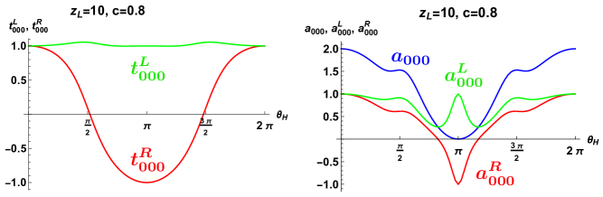
Figure 6: Gauge couplings $t^{R/L}_{000}$and anomaly coefficients $a^{R/L}_{000}$ and $a_{000}$ for $z_{L}=10$ and $c=0.8$ are shown as functions of $\theta_{H}$. The anomaly coefficient $a_{000}$ for $c=0.8$ has the same behavior as $a_{000}$ for $c=0.25$ in Fig. 3.

Let us go back to the expression for $a_{n_{1}n_{2}n_{3}}$ in (5.7) with (5.4).

$$a_{n_{1}n_{2}n_{3}}=\sum_{m,\ell,p}\Big{\{}t_{n_{1}m\ell}^{R}\,t_{n_{2}\ell p}^{R}\,t_{n_{3}pm}^{R}+t_{n_{1}m\ell}^{L}\,t_{n_{2}\ell p}^{L}\,t_{n_{3}pm}^{L}\Big{\}}~{}.$$ (7.1)

There are two ways to evaluate $a_{n_{1}n_{2}n_{3}}$.

Method 1   (i) First evaluate the couplings $t_{nm\ell}^{R/L}\,$. (ii) Then do the summation $\sum_{m\ell p}$.

Method 2   (i) First do the summation $\sum_{m\ell p}$. (ii) Then do the integration $\int dy_{1}dy_{2}dy_{3}$.

So far we have adopted Method 1 to evaluate $a_{n_{1}n_{2}n_{3}}$.

In Method 2 the first step of the summation $\sum_{m\ell p}$ leads to

$$a_{n_{1}n_{2}n_{3}}=\Big{(}\frac{k}{2}\Big{)}^{3}\int\int\int_{-\beta}^{2L-\beta}dy_{1}dy_{2}dy_{3}\,e^{\sigma(y_{1})+\sigma(y_{2})+\sigma(y_{3})}$$ (7.2)

$$\quad\times\Big{[}~{}k_{1}k_{2}k_{3}\big{\{}A_{R}(1,2)A_{R}(2,3)A_{R}(3,1)-B_{R}(1,2)B_{R}(2,3)B_{R}(3,1)$$ (7.3)

$$\hskip 62.59596pt+B_{L}(1,2)B_{L}(2,3)B_{L}(3,1)-A_{L}(1,2)A_{L}(2,3)A_{L}(3,1)\big{\}}$$ (7.4)

$$\qquad+k_{1}h_{2}h_{3}\{\cdots\}+h_{1}k_{2}h_{3}\{\cdots\}+h_{1}h_{2}k_{3}\{\cdots\}\Big{]}~{},$$ (7.5)

$$\quad k_{j}=k_{n_{j}}(y_{j})~{},~{}~{}h_{j}=h_{n_{j}}(y_{j})~{},$$ (7.6)

$$\quad\begin{pmatrix}A_{R/L}(j,k)\cr B_{R/L}(j,k)\end{pmatrix}=\begin{pmatrix}A_{R/L}\cr B_{R/L}\end{pmatrix}(y_{j},y_{k})=\sum_{n=0}^{\infty}\begin{pmatrix}f_{R/Ln}(y_{j})f_{R/Ln}^{*}(y_{k})\cr g_{R/Ln}(y_{j})g_{R/Ln}^{*}(y_{k})\end{pmatrix}.$$ (7.7)

Here we have made use of $\sum_{n=0}^{\infty}f_{R/Ln}(y)g_{R/Ln}^{*}(y^{\prime})=0$. $\beta$ appearing in the integration range in $y_{j}$ is arbitrary. Finding the explicit form of $A_{R/L}$ and $B_{R/L}$ for general $c$ is a difficult task, however.

It is possible to determine $A_{R/L}$ and $B_{R/L}$ for $c=0$. One finds, with $\delta_{L}(x)=\sum_{n}\delta(x-nL)$, that

$$\underline{\hbox{type 1A},~{}c=0}$$ (7.8)

$$A_{R}(y,y^{\prime})=B_{L}(y,y^{\prime})=\frac{e^{-\sigma(y)}}{k}\big{\{}\delta_{2L}(y-y^{\prime})+\delta_{2L}(y+y^{\prime})\big{\}}~{},$$ (7.9)

$$B_{R}(y,y^{\prime})=A_{L}(y,y^{\prime})=\frac{e^{-\sigma(y)}}{k}\big{\{}\delta_{2L}(y-y^{\prime})-\delta_{2L}(y+y^{\prime})\big{\}}~{},$$ (7.10)

Formulas for type 1B are obtained by interchanging $R$ and $L$. Similarly

$$\underline{\hbox{type 2A},~{}c=0}$$ (7.11)

$$A_{R}(y,y^{\prime})=B_{L}(y,y^{\prime})=\frac{e^{-\sigma(y)}}{k}\big{\{}\hat{\delta}_{2L}(y-y^{\prime})+\hat{\delta}_{2L}(y+y^{\prime})\big{\}}~{},$$ (7.12)

$$B_{R}(y,y^{\prime})=A_{L}(y,y^{\prime})=\frac{e^{-\sigma(y)}}{k}\big{\{}\hat{\delta}_{2L}(y-y^{\prime})-\hat{\delta}_{2L}(y+y^{\prime})\big{\}}~{},$$ (7.13)

$$\hat{\delta}_{2L}(y)=\delta_{4L}(y)-\delta_{4L}(y-2L)~{}.$$ (7.14)

Formulas for type 2B are obtained by interchanging $R$ and $L$. When one inserts (7.10) and (7.14) into (7.7), there appear the products of three delta functions in the integrand. With $0<\beta<L$ the products of delta functions reduce to

$$\begin{matrix}\delta_{2L}(y_{1}-y_{2})\delta_{2L}(y_{2}-y_{3})\delta_{2L}(y_{3}+y_{1})\cr\kern 3.0pt\cr\delta_{2L}(y_{1}+y_{2})\delta_{2L}(y_{2}+y_{3})\delta_{2L}(y_{3}+y_{1})\end{matrix}~{}\bigg{\}}$$ (7.15)

$$\quad\Rightarrow\frac{1}{2}\Big{\{}\delta(y_{1})\delta(y_{2})\delta(y_{3})+\delta(y_{1}-L)\delta(y_{2}-L)\delta(y_{3}-L)\Big{\}}~{},$$ (7.16)

$$\begin{matrix}\hat{\delta}_{2L}(y_{1}-y_{2})\hat{\delta}_{2L}(y_{2}-y_{3})\hat{\delta}_{2L}(y_{3}+y_{1})\cr\kern 3.0pt\cr\hat{\delta}_{2L}(y_{1}+y_{2})\hat{\delta}_{2L}(y_{2}+y_{3})\hat{\delta}_{2L}(y_{3}+y_{1})\end{matrix}~{}\bigg{\}}$$ (7.17)

$$\quad\Rightarrow\frac{1}{2}\Big{\{}\delta(y_{1})\delta(y_{2})\delta(y_{3})-\delta(y_{1}-L)\delta(y_{2}-L)\delta(y_{3}-L)\Big{\}}~{}.$$ (7.18)

Furthermore, as $h_{n}(0)=h_{n}(L)=0$, only the terms proportional to $k_{1}k_{2}k_{3}$ in (7.7) survive.

We have arrived at the following formula for the anomaly coefficients;

$$a_{n\ell m}(\theta_{H},z_{L}) =Q_{0}k_{n}(0)k_{\ell}(0)k_{m}(0)+Q_{1}k_{n}(L)k_{\ell}(L)k_{m}(L)~{},$$ (7.19)

where

$$(Q_{0},Q_{1}) =\begin{cases}(+1,+1)&\hbox{for type 1A}\cr(-1,-1)&\hbox{for type 1B}\cr(+1,-1)&\hbox{for type 2A}\cr(-1,+1)&\hbox{for type 2B}\end{cases}~{}.$$ (7.20)

The anomaly coefficients are determined by the values of the wave functions of the gauge fields, $k_{n}(y)$, at the UV and IR branes and the parity, $Q_{j}$, of the right-handed mode of the fermion field.

As observed at the beginning of this section, the anomaly coefficients $a_{n\ell m}(\theta_{H})$ do not depend on the bulk mass parameter $c$ of the fermion field. The anomaly formula (7.19) derived for $c=0$ should apply for other values of $c$. Indeed one can confirm it explicitly. In Fig.  7 $a_{n\ell m}$’s given by the formula (7.19) and those determined by Method 1 for $c=0.25$ are displayed in the case $z_{L}=10$. Blue curves represent the formula (7.19), whereas red dots represent the values determined from the gauge couplings $t_{nm\ell}^{R/L}$ for $c=0.25$. It is seen that the red dots are on the blue curves.

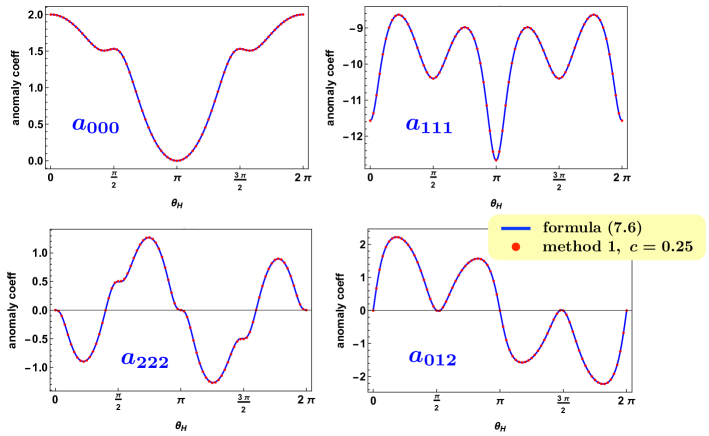
Figure 7: Anomaly coefficients $a_{000}(\theta_{H})$, $a_{111}(\theta_{H})$ , $a_{222}(\theta_{H})$ , $a_{012}(\theta_{H})$ are shown for type 1A fermions with $z_{L}=10$. Blue curves represent the formula (7.19), whereas red dots represent the values determined from the gauge couplings $t_{nm\ell}^{R/L}$ for $c=0.25$ by Method 1.

We stress that the anomaly coefficients depend solely on $k_{n}(0)$, $k_{n}(L)$, $Q_{0}$ and $Q_{1}$. They depend neither on the behavior of the wave functions of gauge fields and fermion field in the bulk region $0<y<L$, nor on the bulk mass parameter $c$ of the fermion field. The formula (7.19) represents holography in anomaly flow. Although each anomaly generated by specific fermion modes running along the internal triangle loop does depend on the detailed behavior of the wave functions of both gauge and fermion fields in the bulk, the total anomaly coefficients, after summing up all possible loop contributions, are determined by the information of the gauge fields at the UV and IR branes and of the parity conditions for the fermion field there.

The formula for the anomaly coefficients $b_{nm\ell}$ in the flat $M^{4}\times(S^{1}/Z_{2})$ spacetime simplifies. As in the RS space, one finds that

$$b_{n\ell m} =Q_{0}k^{\rm flat}_{n}(0)k^{\rm flat}_{\ell}(0)k^{\rm flat}_{m}(0)+Q_{1}k^{\rm flat}_{n}(L)k^{\rm flat}_{\ell}(L)k^{\rm flat}_{m}(L)~{}.$$ (7.21)

In the flat space $k_{n}^{\rm flat}(y)=\cos(n\pi y/L)$ so that

$$b_{n\ell m} =Q_{0}+(-1)^{n+\ell+m}\,Q_{1}~{},$$ (7.22)

which agrees with (4.6) with $Q_{0}=Q_{1}=1$ for a doublet fermion of type 1A.

8 Anomaly cancellation

In gauge theory in four dimensions gauge anomalies have to be cancelled for the consistency of the theory. In GHU the holography in anomaly flow becomes crucial to guarantee the cancellation of gauge anomalies. In the SM all gauge anomalies are cancelled among quarks and leptons in each generation.[12, 13]

In the $SU(2)$ GHU under consideration one may introduce several fermion doublets, each of which has its own bulk mass parameter $c$. Let the numbers of doublet fermions of type 1A, 1B, 2A and 2B be $n_{1A}$, $n_{1B}$, $n_{2A}$ and $n_{2B}$, respectively. It follows from (7.19) that the anomalies are cancelled if

$$n_{1A}=n_{1B}~{},~{}~{}n_{2A}=n_{2B}~{},$$ (8.1)

as the anomaly coefficients do not dependon $c$. The condition is generalized in the presence of brane fermions, namely fermions living only on the UV or IR brane. Suppose that there are $\hat{n}_{R}$ right-handed and $\hat{n}_{L}$ left-handed doublet brane fermions on the UV brane at $y=0$. As the $Z_{\mu}^{(n)}$ coupling of each brane fermion is given by $(g_{4}/2)\,k_{n}(0)$, the anomaly cancellation conditions become

$$n_{1A}-n_{1B}+n_{2A}-n_{2B}+\hat{n}_{R}-\hat{n}_{L}=0~{},$$ (8.2)

$$n_{1A}-n_{1B}-n_{2A}+n_{2B}=0~{},$$ (8.3)

It is important that the conditions (8.1) and (8.3) do not depend on $\theta_{H}$ and $z_{L}$. The conditions guarantee that not only the zero mode anomaly $a_{000}$ but also all other anomalies $a_{n\ell m}$ are cancelled at once. In GHU in the RS space the gauge couplings vary as $\theta_{H}$, which further depends on $c$, or on the fermion species, but the anomaly cancellation conditions do not depend on $\theta_{H}$.

9 Summary

We have shown that the anomaly flows with the AB phase $\theta_{H}$. In the RS space everything changes smoothly with $\theta_{H}$. In the $SU(2)$ GHU model in the RS space a chiral fermion at $\theta_{H}=0$ is transformed to a vector-like fermion at $\theta_{H}=\pi$. The magnitude of the anomaly coming from one fermion doublet varies with $\theta_{H}$. The total anomaly coefficients $a_{nm\ell}(\theta_{H})$ are given by thec formula (7.19), which represents holography in anomaly flow.

The anomalies can be cancelled among several fermion doublets. The cancellation conditions are given by (8.1) or (8.3). They are independent of $\theta_{H}$ and $z_{L}$, which is important to achieve the anomaly cancellation in the realistic GHU models in the RS space. The examination of anomaly cancellation in the $SO(5)\times U(1)_{X}\times SU(3)_{C}$ GHU in the RS space is necessary.

In this connection one may worry about the fact that the gauge couplings vary with $\theta_{H}$, and the couplings of quarks and leptons are not purely chiral at $\theta_{H}\not=0$. In the SM only left-handed quark-lepton doublets couple to $W$. In GHU models in the RS space right-handed components also have small couplings to $W$ at $\theta_{H}\not=0$. The detailed study of the GUT inspired $SO(5)\times U(1)_{X}\times SU(3)_{C}$ GHU has been done recently.[14]. In the realistic model $\theta_{H}\sim 0.1$, $m_{\rm KK}\sim 13\,$TeV and $z_{L}\sim 4\times 10^{11}$. The $W$ couplings of right-handed quarks in units of $g_{w}$ are $O(10^{-12})$, $O(10^{-9})$, and $O(10^{-5})$ for $(u,d)$, $(c,s)$ and $(t,b)$, respectively. The $W$ couplings of right-handed leptons are much smaller.

Anomaly flow by an Aharonov-Bohm phase is a new phenomenon, which is different from the phenomenon of anomaly inflow.[15, 16, 17] Further investigation is desired.

Appendix A Basis functions

Wave functions of gauge fields and fermions in the RS space are expressed in terms of the Bessel functions. For gauge fields we introduce

$$C(z;\lambda) =\frac{\pi}{2}\lambda zz_{L}F_{1,0}(\lambda z,\lambda z_{L})~{},$$ (A.1)

$$S(z;\lambda) =-\frac{\pi}{2}\lambda zF_{1,1}(\lambda z,\lambda z_{L})~{},$$ (A.2)

$$C^{\prime}(z;\lambda) =\frac{\pi}{2}\lambda^{2}zz_{L}F_{0,0}(\lambda z,\lambda z_{L})~{},$$ (A.3)

$$S^{\prime}(z;\lambda) =-\frac{\pi}{2}\lambda^{2}zF_{0,1}(\lambda z,\lambda z_{L})~{},$$ (A.4)

$$F_{\alpha,\beta}(u,v) \equiv J_{\alpha}(u)Y_{\beta}(v)-Y_{\alpha}(u)J_{\beta}(v)~{},$$ (A.5)

where $J_{\alpha}(u)$ and $Y_{\alpha}(u)$ are Bessel functions of the first and second kind. These functions satisfy

$$-z\frac{d}{dz}\frac{1}{z}\frac{d}{dz}\begin{pmatrix}C\cr S\end{pmatrix}=\lambda^{2}\begin{pmatrix}C\cr S\end{pmatrix}~{},~{}~{}-\frac{d}{dz}z\frac{d}{dz}\frac{1}{z}\begin{pmatrix}C^{\prime}\cr S^{\prime}\end{pmatrix}=\lambda^{2}\begin{pmatrix}C^{\prime}\cr S^{\prime}\end{pmatrix}~{},$$ (A.6)

$$C(z_{L};\lambda)=z_{L}~{},~{}~{}C^{\prime}(z_{L};\lambda)=0~{},~{}~{}S(z_{L};\lambda)=0~{},~{}~{}S^{\prime}(z_{L};\lambda)=\lambda~{},$$ (A.7)

$$CS^{\prime}-SC^{\prime}=\lambda z~{}.$$ (A.8)

For fermion fields with a bulk mass parameter $c$, we define

$$\begin{pmatrix}C_{L}\cr S_{L}\end{pmatrix}(z;\lambda,c) =\pm\frac{\pi}{2}\lambda\sqrt{zz_{L}}F_{c+\frac{1}{2},c\mp\frac{1}{2}}(\lambda z,\lambda z_{L})~{},$$ (A.9)

$$\begin{pmatrix}C_{R}\cr S_{R}\end{pmatrix}(z;\lambda,c) =\mp\frac{\pi}{2}\lambda\sqrt{zz_{L}}F_{c-\frac{1}{2},c\pm\frac{1}{2}}(\lambda z,\lambda z_{L})~{}.$$ (A.10)

These functions satisfy

$$D_{+}(c)\begin{pmatrix}C_{L}\cr S_{L}\end{pmatrix}=\lambda\begin{pmatrix}S_{R}\cr C_{R}\end{pmatrix},$$ (A.11)

$$D_{-}(c)\begin{pmatrix}C_{R}\cr S_{R}\end{pmatrix}=\lambda\begin{pmatrix}S_{L}\cr C_{L}\end{pmatrix},~{}~{}D_{\pm}(c)=\pm\frac{d}{dz}+\frac{c}{z}~{},$$ (A.12)

$$C_{R}=C_{L}=1~{},~{}~{}S_{R}=S_{L}=0\quad{\rm at~{}}z=z_{L}~{},$$ (A.13)

$$C_{L}C_{R}-S_{L}S_{R}=1~{}.$$ (A.14)

Appendix B Wave functions in RS

The wave functions $\tilde{\bf h}_{n}(z)\equiv(\tilde{h}_{n}(z),\tilde{k}_{n}(z))^{t}$ in (3.8) for gauge fields are given by

$$\tilde{\bf h}_{0}(z)=\bar{\bf h}_{0}^{a}(z)~{},$$ (B.1)

$$[\tilde{\bf h}_{2\ell-1}(z),\tilde{\bf h}_{2\ell}(z)]=(-1)^{\ell}\begin{cases}[\bar{\bf h}_{2\ell-1}^{a}(z),\bar{\bf h}_{2\ell}^{b}(z)]&{\rm for}-\frac{1}{2}\pi<\theta_{H}<\frac{1}{2}\pi\cr[\bar{\bf h}_{2\ell-1}^{b}(z),-\bar{\bf h}_{2\ell}^{a}(z)]&{\rm for~{}}0<\theta_{H}<\pi\cr[-\bar{\bf h}_{2\ell-1}^{a}(z),-\bar{\bf h}_{2\ell}^{b}(z)]&{\rm for~{}}\frac{1}{2}\pi<\theta_{H}<\frac{3}{2}\pi\cr[-\bar{\bf h}_{2\ell-1}^{b}(z),\bar{\bf h}_{2\ell}^{a}(z)]&{\rm for~{}}\pi<\theta_{H}<2\pi\cr[\bar{\bf h}_{2\ell-1}^{a}(z),\bar{\bf h}_{2\ell}^{b}(z)]&{\rm for~{}}\frac{3}{2}\pi<\theta_{H}<\frac{5}{2}\pi\end{cases}$$ (B.2)

$$\hskip 99.58464pt(\ell=1,2,3,\cdots)~{},$$ (B.3)

$$\bar{\bf h}_{n}^{a}(z)=\frac{1}{\sqrt{r^{a}_{n}}}\begin{pmatrix}-\sin\theta_{H}\hat{S}(z;\lambda_{n})\cr\cos\theta_{H}C(z;\lambda_{n})\end{pmatrix},~{}~{}\bar{\bf h}_{n}^{b}(z)=\frac{1}{\sqrt{r^{b}_{n}}}\begin{pmatrix}\cos\theta_{H}S(z;\lambda_{n})\cr\sin\theta_{H}\check{C}(z;\lambda_{n})\end{pmatrix},$$ (B.4)

$$\hskip 28.45274pt\hat{S}(z;\lambda)=\frac{C(1;\lambda)}{S(1;\lambda)}\,S(z;\lambda)~{},~{}~{}\check{C}(z;\lambda)=\frac{S^{\prime}(1;\lambda)}{C^{\prime}(1;\lambda)}\,C(z;\lambda)~{},$$ (B.5)

$$\hskip 28.45274ptr_{n}=\frac{1}{kL}\int_{1}^{z_{L}}\frac{dz}{z}\big{\{}|\hat{h}_{n}(z)|^{2}+|\hat{k}_{n}(z)|^{2}\big{\}}\quad{\rm for}~{}\begin{pmatrix}\hat{h}_{n}(z)\cr\hat{k}_{n}(z)\end{pmatrix}.$$ (B.6)

In (B.6) two expressions in an overlapping region in $\theta_{H}$ are the same.

The wave functions $\tilde{\bf f}_{Rn}(z)=(\tilde{f}_{Rn}(z),\tilde{g}_{Rn}(z))^{t}$ and $\tilde{\bf f}_{Ln}(z)=(\tilde{f}_{Ln}(z),\tilde{g}_{Ln}(z))^{t}$ in (3.15) for fermion fields of type 1A with $c\geq 0$ are given by

$$[\tilde{\bf f}_{R,2\ell}(z),\tilde{\bf f}_{R,2\ell+1}(z)] =\begin{cases}[\bar{\bf f}_{R,2\ell}^{a}(z),\bar{\bf f}_{R,2\ell+1}^{c}(z)]&{\rm for~{}}-\pi<\theta_{H}<\pi\cr[\bar{\bf f}_{R,2\ell}^{b}(z),\bar{\bf f}_{R,2\ell+1}^{d}(z)]&{\rm for~{}}0<\theta_{H}<2\pi\cr[-\bar{\bf f}_{R,2\ell}^{a}(z),-\bar{\bf f}_{R,2\ell+1}^{c}(z)]&{\rm for~{}}\pi<\theta_{H}<3\pi\cr[-\bar{\bf f}_{R,2\ell}^{b}(z),-\bar{\bf f}_{R,2\ell+1}^{d}(z)]&{\rm for~{}}2\pi<\theta_{H}<4\pi\cr[\bar{\bf f}_{R,2\ell}^{a}(z),\bar{\bf f}_{R,2\ell+1}^{c}(z)]&{\rm for~{}}3\pi<\theta_{H}<5\pi\cr\end{cases}$$ (B.7)

$$\hskip 28.45274pt(\ell=0,1,2,\cdots)~{},$$ (B.8)

$$\tilde{\bf f}_{L0}(z) =\bar{\bf f}_{L0}^{a}(z),$$ (B.9)

$$[\tilde{\bf f}_{L,2\ell-1}(z),\tilde{\bf f}_{L,2\ell}(z)] =\begin{cases}[\bar{\bf f}_{L,2\ell-1}^{a}(z),\bar{\bf f}_{L,2\ell}^{c}(z)]&{\rm for~{}}-\pi<\theta_{H}<\pi\cr[\bar{\bf f}_{L,2\ell-1}^{b}(z),\bar{\bf f}_{L,2\ell}^{d}(z)]&{\rm for~{}}0<\theta_{H}<2\pi\cr[-\bar{\bf f}_{L,2\ell-1}^{a}(z),-\bar{\bf f}_{L,2\ell}^{c}(z)]&{\rm for~{}}\pi<\theta_{H}<3\pi\cr[-\bar{\bf f}_{L,2\ell-1}^{b}(z),-\bar{\bf f}_{L,2\ell}^{d}(z)]&{\rm for~{}}2\pi<\theta_{H}<4\pi\cr[\bar{\bf f}_{L,2\ell-1}^{a}(z),\bar{\bf f}_{L,2\ell}^{c}(z)]&{\rm for~{}}3\pi<\theta_{H}<5\pi\cr\end{cases}$$ (B.10)

$$\hskip 28.45274pt(\ell=1,2,3,\cdots)~{}.$$ (B.11)

Here

$$\bar{\bf f}_{Rn}^{a}(z)=\frac{1}{\sqrt{r^{a}_{n}}}\begin{pmatrix}\cos\hbox{$\frac{1}{2}$}\theta_{H}C_{R}(z;\lambda_{n},c)\cr-\sin\hbox{$\frac{1}{2}$}\theta_{H}\hat{S}_{R}(z;\lambda_{n},c)\end{pmatrix},~{}~{}\bar{\bf f}_{Rn}^{b}(z)=\frac{1}{\sqrt{r^{b}_{n}}}\begin{pmatrix}\sin\hbox{$\frac{1}{2}$}\theta_{H}C_{R}(z;\lambda_{n},c)\cr\cos\hbox{$\frac{1}{2}$}\theta_{H}\check{S}_{R}(z;\lambda_{n},c)\end{pmatrix},$$ (B.12)

$$\bar{\bf f}_{Rn}^{c}(z)=\frac{1}{\sqrt{r^{c}_{n}}}\begin{pmatrix}\sin\hbox{$\frac{1}{2}$}\theta_{H}\hat{C}_{R}(z;\lambda_{n},c)\cr\cos\hbox{$\frac{1}{2}$}\theta_{H}S_{R}(z;\lambda_{n},c)\end{pmatrix},~{}~{}\bar{\bf f}_{Rn}^{d}(z)=\frac{1}{\sqrt{r^{d}_{n}}}\begin{pmatrix}-\cos\hbox{$\frac{1}{2}$}\theta_{H}\check{C}_{R}(z;\lambda_{n},c)\cr\sin\hbox{$\frac{1}{2}$}\theta_{H}S_{R}(z;\lambda_{n},c)\end{pmatrix},$$ (B.13)

$$\bar{\bf f}_{Ln}^{a}(z)=\frac{1}{\sqrt{r^{a}_{n}}}\begin{pmatrix}\sin\hbox{$\frac{1}{2}$}\theta_{H}\hat{S}_{L}(z;\lambda_{n},c)\cr\cos\hbox{$\frac{1}{2}$}\theta_{H}C_{L}(z;\lambda_{n},c)\end{pmatrix},~{}~{}\bar{\bf f}_{Ln}^{b}(z)=\frac{1}{\sqrt{r^{b}_{n}}}\begin{pmatrix}-\cos\hbox{$\frac{1}{2}$}\theta_{H}\check{S}_{L}(z;\lambda_{n},c)\cr\sin\hbox{$\frac{1}{2}$}\theta_{H}C_{L}(z;\lambda_{n},c)\end{pmatrix},$$ (B.14)

$$\bar{\bf f}_{Ln}^{c}(z)=\frac{1}{\sqrt{r^{c}_{n}}}\begin{pmatrix}\cos\hbox{$\frac{1}{2}$}\theta_{H}S_{L}(z;\lambda_{n},c)\cr-\sin\hbox{$\frac{1}{2}$}\theta_{H}\hat{C}_{L}(z;\lambda_{n},c)\end{pmatrix},~{}~{}\bar{\bf f}_{Ln}^{d}(z)=\frac{1}{\sqrt{r^{d}_{n}}}\begin{pmatrix}\sin\hbox{$\frac{1}{2}$}\theta_{H}S_{L}(z;\lambda_{n},c)\cr\cos\hbox{$\frac{1}{2}$}\theta_{H}\check{C}_{L}(z;\lambda_{n},c)\end{pmatrix},$$ (B.15)

$$\qquad r_{n}=\int_{1}^{z_{L}}dz\big{\{}|\hat{f}_{n}(z)|^{2}+|\hat{g}_{n}(z)|^{2}\big{\}}\quad{\rm for}~{}\begin{pmatrix}\hat{f}_{n}(z)\cr\hat{g}_{n}(z)\end{pmatrix},$$ (B.16)

and

$$\begin{pmatrix}\hat{S}_{L}\cr\hat{C}_{R}\end{pmatrix}(z;\lambda,c)=\frac{C_{L}(1;\lambda,c)}{S_{L}(1;\lambda,c)}\begin{pmatrix}S_{L}\cr C_{R}\end{pmatrix}(z;\lambda,c),~{}~{}\begin{pmatrix}\hat{C}_{L}\cr\hat{S}_{R}\end{pmatrix}(z;\lambda,c)=\frac{C_{R}(1;\lambda,c)}{S_{R}(1;\lambda,c)}\begin{pmatrix}C_{L}\cr S_{R}\end{pmatrix}(z;\lambda,c),$$ (B.17)

$$\begin{pmatrix}\check{S}_{L}\cr\check{C}_{R}\end{pmatrix}(z;\lambda,c)=\frac{S_{R}(1;\lambda,c)}{C_{R}(1;\lambda,c)}\begin{pmatrix}S_{L}\cr C_{R}\end{pmatrix}(z;\lambda,c),~{}~{}\begin{pmatrix}\check{C}_{L}\cr\check{S}_{R}\end{pmatrix}(z;\lambda,c)=\frac{S_{L}(1;\lambda,c)}{C_{L}(1;\lambda,c)}\begin{pmatrix}C_{L}\cr S_{R}\end{pmatrix}(z;\lambda,c).$$ (B.18)

In (B.11) two expressions in an overlapping region in $\theta_{H}$ are the same.

References