Control the qubit-qubit coupling in the superconducting circuit with double-resonator couplers
Abstract
We propose a theoretical scheme of using two-fixed frequency resonator couplers to tune the interaction between two Xmon qubits. The indirect interaction between two qubits induced by two resonators can cancel each other, so the direct qubit-qubit coupling is not essential for the switching off. So we can suppress the static ZZ coupling with the weak direct qubit-qubit coupling and even eliminate the static ZZ coupling through the destructive interferences of the double-path couplers. The cross-kerr resonance can induce additional poles for the static ZZ coupling which should be kept away during the two-qubit gates. The double-resonator couplers scheme could unfreeze some restrictions during the design of superconducting quantum chips and mitigate the static ZZ coupling, which might supply a promising platform for future superconducting quantum chip.
I Introduction
In past several years, the superconducting quantum computing develops quickly, IBM announced 433 qubits superconducting quantum chip at the end of 2022, and plan to launch quantum chip with more than 1000 qubits in 2023. The coherence time of superconducting qubits fabricated with new superconducting materials is greatly enhanced[1, 2, 3, 4, 5], and the introduction of tunable coupler greatly enhances the fidelities of two-qubit gates to above [6, 7, 8, 9, 12, 10, 11]. The quantum supremacy of random circuit sampling and other multi-body quantum simulation experiments have been conducted on the superconducting quantum chip with more than 50 qubits [14, 15, 13, 4]. But the fidelities of two-qubit gate are still not high enough for the universal quantum computer, and the state leakages and residual coupling are still need to be suppressed in superconducting qunatum chip.
The tunable coupler can switch off the interactions between adjacent qubits, which can isolate qubits from the surrounding environments for local quantum operations. In the single-coupler circuit, the induced indirect qubit-qubit coupling (dispersive type interaction) can not be zero for finite frequency detuning between qubit and coupler, so the direct qubit-qubit interaction is required for switching off. If the direct qubit-qubit coupling is very weak, the switching off frequency should be very high, and this leaves narrow available frequency ranges for readout resonators (or qubits). For the case of strong direct qubit-qubit coupling, the state leakages and crosstalks should be another perplex[6, 7, 8]. So there are many limitations during the design of single-coupler superconducting quantum chip, and the residual coupling and state leakages are still serious troubles[16].
In this article, we propose a theoretical scheme to dynamically tune the qubit-qubit coupling with the double-resonator couplers in the superconducting quantum chip. As theoretically and experimentally demonstrated, the superconducting resonator can function as a coupler[17, 20, 18, 19, 22, 21]. In particular, if the two resonator couplers take the respective maximal and minimal frequencies, the induced indirect qubit-qubit coupling by two resonators are in opposite signs and can cancel each other. So the direct qubit-qubit couplings is not indispensable for switching off in the double-resonator coupler circuit, which can hopefully unfreeze some restrictions on the superconducting quantum chip, such as the qubit-qubit coupling strengths, maximal frequencies of couplers, and so on. The switching off positions can be very close to two-qubit gate regimes in the double-resonator couplers circuit, thus the maximal frequencies of couplers can be smaller. So available frequency ranges for readout resonators or qubits can be wider in double-path coupler circuit, and this should relieve the frequency crowding on the superconducting quantum chip.
We also study the effects of superconducting artificial atom’s high-excited states on qubits’ energy levels and switching off positions. The elimination of the static ZZ coupling through the destructive interferences of double-path couplers are also explored[23, 24, 12, 25]. We find that the cross-kerr resonances through the virtual photon exchange could induce new poles of the static ZZ coupling, which should be kept away from during the two-qubit gates.
The paper is organized as follows: In Sec. II, we first perform Numerical calculation of the circuit energy levels. In Sec. III, we then discuss the Switching off for the qubit-qubit coupling. In Sec. IV, we further study the suppression and cancellation of Static ZZ coupling. Finally, we summarize the results in Sec. V.
II Circuit Energy levels
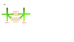
In this section, we numerically calculate the energy levels of qubits for the superconducting circuit in Fig. 1 with the QuTiP software [26, 27, 28, 16]. The superconducting circuit consists of two Xmon qubits coupling to two common resonator couplers. The two-body interactions are all assumed as capacitive type, and the direct qubit-qubit and resonator-resonator interactions are very weak. The two-body interactions in the superconducting circuit are all assumed as capacitive type. Because of the small anharmonicities, the high-excited states of superconducting artificial atoms should also make contributions to the energy levels of qubits and couplers. Truncated to the second-excited states of atoms and third-excited states of resonators, the curved surfaces of qubits and resonators’ energy levels are plotted in Appendix A (see Fig. 10).
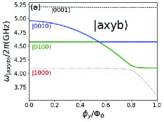
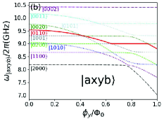
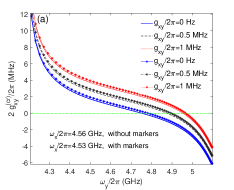
For simplicity, we focus on the special case that the resonant frequency of resonator a, resonant frequency of resonator b , and the transition frequency of qubit x are fixed, and only the transition frequency for qubit y is tuned by the external magnetic flux . By setting GHz, the energy level curves of qubits and resonators’ single and double-excited states are plotted in Figs.2(a) and 2(b), respectively. During the numerical calculations with QuTiP software , the transition frequencies of qubit x and qubit y are respectively chosen as GHz and GHz, the resonant frequencies of resonator a and resonator b are GHz and GHz, respectively. The coupling strengths between resonator a (or b) and two qubits are MHz (or MHz), so the qubits and couplers are in the dispersive coupling regimes.
The ket vector of four-body quantum state is defined as , and the values of respectively describe quantum numbers of resonator a, qubit x, qubit y, and resonator b. Because of the avoided crossing effect, each curve in Fig. 2 can not describe the whole energy level of a certain quantum state, here we mark each curve with the corresponding state at the zero magnetic flux. In Fig.2(a), the transition frequency of qubit y decreases under magnetic field, and it becomes anticrossing with qubit x at the frequency regimes close to 4.56 GHz and with resonator a at the regimes close to 4.10 GHz. For the double-excited states, the energy levels and avoided crossing gaps can be seen in Fig. 2(b). The energy level structure in Fig.2 is important for analyzing the switching off and the static ZZ coupling on the superconducting quantum chip as shown in the follow sections.
III switching off
III.1 Circuit Quantization
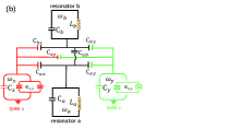
Figure 1(a) describes the superconducting circuit consisting of two Xmon qubits coupling to two common fixed frequency resonators, the frequencies of qubits are tunable. Besides the direct interactions, the qubit-resonator couplings can also induce indirect qubit-qubit and resonator-resonator interactions. The resonant frequencies of resonators a and b are respective and , while and label the transition frequencies of qubits x and y, respectively. In the case of zero magnetic fluxes, the frequencies of qubits and resonators satisfy . We expect a large distance between two resonators and neglect their inductive coupling, then the interactions are all regarded as capacitive type as shown in Fig. 1(b). The capacitances of resonators should be distributed type and proportional to their lengths, but in the article we simply label the total capacitances of resonators a and b as and , respectively.
Inspired by previous work[17, 20], the kinetic energy of superconducting circuit with double-resonator couplers can be written as , where is the capacitance of qubit or resonator, and () is relative capacitance between arbitrary two devices among qubits and resonators, with and . The and are the respective magnetic fluxes of circuit nodes for resonators a and b, while and are the respective node fluxes of qubits x and y, and they can be tuned by the external magnetic fluxes and [29, 30, 31]. If we label the and as the respective inductances of resonators a and b, thus the potential energy of superconducting circuit can be written as , the subscript label the respective variables of resonators a and b, while describe the variables of qubit x and qubit y, respectively. The is the Josephson energy of qubit , where the is the corresponding critical current, and is the flux quantum with the planck constant h and an electron charge e.
With the kinetic energy and potential energy , the Lagrangian of the superconducting circuit in Fig. 1 can be formally written as . If we define the generalized momentum operators as (with ), under the conditions , we obtain the expression of Hamiltonian (see Appendix B)
where is the Cooper-pair number operator of a qubit or resonator, and the corresponding charging energy is . The transition frequencies of resonators and qubits are respectively defined as and , while labels the anharmonicity of qubit . As shown in Appendix B, the two-body coupling strengths among qubits and resonators can be defined as
| (2) | |||||
| (3) | |||||
| (4) |
The two-body interactions are mainly decided by their relative capacitances with and . The qubit-resonator coupling strength in Eq.(2) could induce indirect interaction between two qubits, so the Eq. (4) can not describe the complete interaction between two qubits. In the single-coupler superconducting quantum chip, there are many restrictions on the capacitances and frequencies of qubits (or couplers), but these limitations might be unfrozen in the double-coupler circuit as will be discussed in the follow sections.
III.2 Effective coupling
To get the effective qubit-qubit coupling, we try to decouple the qubit-resonator interactions in this section. For the Xmon qubit, the Josephson energy is much larger than its charging energy, , and then the should be very small and we can use the approximate equation: . If we introduce the creation and annihilation operators by the definitions , and , the second-quantization Hamiltonian can be obtained as , with
| (5) | |||||
| (6) | |||||
| (7) | |||||
| (8) | |||||
| (9) |
We define to describe anharmonicity of qubit , and the nonlinear term reflects the effects of high-excited states of superconducting artificial atom. We define the to describe the frequency detuning between the qubit and resonator , while is the frequency summation of qubit and resonator . describes the frequency detuning between two qubits, and labels the frequency detuning between two resonators.
Separating the Hamiltonian as , the free term is defined as , while the interaction term is . In the qubit-resonator dispersive coupling regimes and , we define . Under the Schrieffer–Wolff transformation, if we choose and , thus the decoupled Hamiltonian becomes (see Appendix C), that is
| (10) | |||||
Since , the contributions of and have been neglected. Following the method of previous work[7], we assumed during the derivations of Eq.(10), thus the contributions of superconducting artificial atoms’ high-excited states are neglected.
The decoupled frequencies of qubits and resonators can be respectively defined as and (as shown in Appendix C,). And the decoupled qubit-qubit coupling strength can be obtained as
| (11) |
Since and depend the frequency of qubit , so the induced qubit-qubit coupling can be tuned by the external magnetic fluxes and . To switch off the qubit-qubit coupling ( Hz), we should find parameters to satisfy .
From the expression of , both two resonators make contributions to the effective qubit-qubit coupling, and their contributions might cancel each other () if the qubit frequency of qubits satisfy certain conditions. Thus the direct qubit-qubit coupling might be not necessary for the switching off in the double-resonator couplers circuit. The qubits could also induce indirect interactions between the two resonators, and the decoupled resonator-resonator coupling strength can be defined as (see Appendix C). Because of the large frequency detuning between two resonators (), the effective resonator-resonator interaction makes little effect on the energy levels of qubits and resonators.
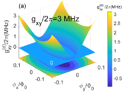
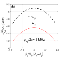
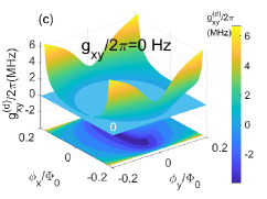
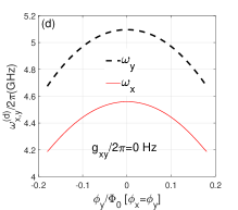
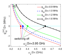
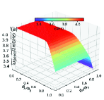
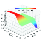
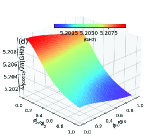
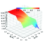
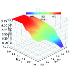
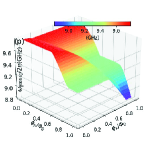
With the parameters in Fig. 2, we can get and in the idling states of qubits (without external magnetic field). This means that the qubits and resonators are in the dispersive or weak-dispersive coupling regimes, thus the perturbation method can be used to calculate the effective qubit-qubit coupling . If we choose , the signs of and are opposite. As indicated by , the resonator b will induce negative indirect qubit-qubit coupling, and the contributions of resonators a is positive. With Eq. (11), the curved surfaces of are plotted in Figs. 3(a) and 3(c), and the corresponding decoupled frequencies of qubits are shown in Figs. 3(b) and 3(d). The curved surface of has many crossing points with the zero value plane ( Hz) in Fig. 3(a) ( MHz), which correspond to switch off positions for the qubit-qubit coupling. The multiple switching off points can be used to optimize the quantum operation parameters and reduce the effects of adjoint qubits. For the case of nonzero direct qubit-qubit coupling (), the distribution of crossing points forms an approximately elliptical curve in - plane as shown in Fig. 3(a), and this means that the contributions of resonator b to induced qubit-qubit coupling (in amplitudes) is larger than the contributions of resonator a.
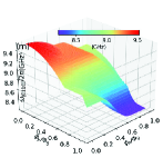
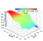
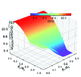
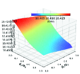
In the case of Hz, the effective qubit-qubit can also be zero if the indirect qubit-qubit couplings induced by resonators a and b are the same in amplitudes but opposite in signs (). As shown in Fig. 3(c), the curved surface of can also cross with the zero values plane ( Hz) in the case of Hz, and this means that the switching off can be realized without the direct qubit-qubit interaction in the double-resonator couplers circuit. The distribution of switching off points approximately forms a circle in - plane in Fig. 3(c), which indicates the approximate equal contributions (in amplitudes) of two resonators to the effective qubit-qubit couplings. The decoupled frequencies of qubits are plotted in Fig. 3(b) ( MHz) and Fig. 3(d)( Hz), and the effects of direct qubit-qubit coupling to the transition frequencies of qubits seems not very large.
The switching off positions are not totally decided by the direct qubit-qubit coupling in the double-resonator coupler circuit, thus we can take arbitrary small or even zero direct qubit-qubit coupling strength in principally, which might be helpful to suppress the state leakages and crosstalks on the superconducting quantum chips. And the restrictions on the direct qubit-qubit coupling strength and coupler’s frequency can be unfreezed on the double-resonator couplers superconducting quantum chip). If we choose the switching off positions close to two-qubit gate regimes, thus the maximal frequencies of couplers can be smaller, and this might create wider available frequency ranges for the readout resonators and relieve the frequency crowding on the superconducting quantum chip.
III.3 High-excited states corrections
In current theoretical model for tunable coupler circuit, the nonlinear term term is regarded as invariant during dynamical decoupling processes for qubit-resonator interactions[7, 16]. This approximation in fact neglects the effects of superconducting artificial atoms’ high-excited states, so the in Eq. (11) does not contain the information of anharmonicity . Because of the small anharmonicity for Xmon qubit (between 200 MHz and 400 MHz), the interactions between the resonators and high-excited states of superconducting artificial atoms should make corrections to the qubits’ energy levels and effective qubit-qubit coupling.
The Bogoliubov transformation has been used to analyze the variations of nonlinear term during the decoupling processes[40, 39], and the derived self-kerr and cross-kerr resonant terms under the unitary transformation reflect the contributions of superconducting artificial atoms’ high-excited states. To maintain consistency, in this section we continue to use the Schrieffer–Wolff transformation to calculate the effects of the nonlinear term (see appendix D). In the qubit-resonator dispersive coupling regimes, and , we define with . Since is a small quantity, we will separately conduct the Unitary transform to study its contributions to the high-order effects, such as cross-kerr resonance, self-kerr resonance, and so on[40]. With tedious calculations (see Appendix D), up to the second-order perturbation expansion terms, we get
Since , the indirect interaction induced by the weakly direct qubit-qubit and resonator-resonator interactions have been neglected. The first and second lines in the right side of Eq.(12) respectively describe the self-kerr and cross-kerr resonance terms, and the complete calculation results can be seen in Appendix D. There are no external pump fields for resonator couplers, so the cavity photon numbers should be very small (). Thus we can get the approximate frequency shift for qubit induced by the nonlinear terms,
| (13) |
We can see that the frequency shift for qubit is proportional to the qubit’s anharmonicity , which reflects the effects of the second-excited state of superconducting artificial atoms. Adding the frequency shift induced by the nonlinear term , we can approximately get the corrected frequency of qubit in decoupled coordinate frame
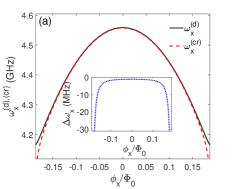
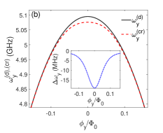
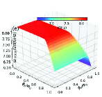
The transition frequency of qubit x in decoupled coordinate is plotted in Fig. 4(a), the deviation between and is larger at the regimes far from the zero magnetic flux points, which coincides with the curve of in insert figure. On the contrary, the maximal deviation between and appears at the regime close to the zero magnetic flux ( or ) in Fig. 4(b), this also coincides with the curve of in the insert figure.
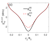
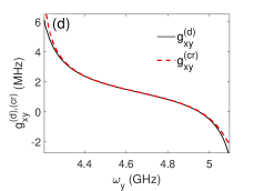
If we replace the with in Eq.(11), we can get the corrected effective qubit-qubit coupling . The resonators’ resonant frequencies and are fixed in this article, so the effective qubit-qubit coupling are mainly tuned by the qubits’ transition frequencies and . By setting GHz, we plot the curves of effective qubit-qubit coupling and on the respective and in Figs. 4(c) and 4(d), the points satisfying Hz or Hz corresponds to the switching off position for the qubit-qubit interaction. The zero value points of and are different, which reflects the effects of the nonlinear term ( also the second-excited state of superconducting artificial atom) on the switching off positions. The calculation results of the corrections to qubits’ frequencies and effective qubit-qubit coupling strength can help to accurately design the superconducting quantum chip.
III.4 Switching off the qubit-qubit coupling
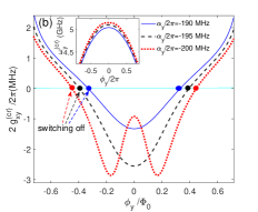
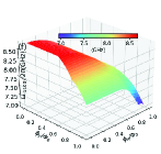
In this section, we study the effects of direct qubit-qubit coupling and qubit’s anharmonicitiy on the effective qubit-qubit coupling and the switching off position. If we take the parameters of Fig. 2, we can get and in the idling states of qubits (without external magnetic field), so the qubits and resonators are in the dispersive or weak-dispersive coupling regimes. To see clearer the working mechanism of switching-off processes in the double-resonator couplers circuit, we plot the one-dimensional curves of effective qubit-qubit coupling with the variation of qubit transition frequency in Fig. 5(a). By fixing GHz, the three curves without markers in Fig. 5(a) correspond to different direct qubit-qubit coupling strengths: Hz in the blue-solid curve, MHz in black-dashed curve, and MHz in the red-dotted curve. The crossing points of three curves with zero value line ( Hz) are different, this means that the direct qubit-qubit coupling could affect the switching off positions. If we set GHz, the switching off points in the three marked curves show considerable shifts relative to the corresponding same color curves without markers.
In Fig. 5(b), we plot the curves of effective qubit-qubit coupling on the node phase with GHz. For the same ranges of node phase , the qubit’s maximal frequencies are not the same for different anharmonicities as shown in the insert figure. For different anhamonicities , the shifts of switching off positions on three curves reflect the effects of superconducting artificial atom’s second-excited states.
The frequency of qubit y should be tuned close to for the iSWAP gate and for the Controlled-Z gate. For the single-path coupler circuit, the switching off point is usually close to the idling coupler frequency (usually about 6.0 GHz) which is far from the two-qubit gate regimes (usually below 5.0 GHz). In the double-resonator couplers circuit, the switching off positions can be very close to the two-qubit gate regimes as shown in Fig. 5(a). So the maximal frequencies of couplers can be smaller in the double-resonator couplers superconducting circuit, this leaves wider available ranges for readout resonators (or qubits) and might relieve the frequency crowding on superconducting quantum chip.
IV Static ZZ coupling
The tunable coupler could isolate the qubits from surrounding environments for local quantum operations and reduce the accumulated phases for the quantum state preparations, and this can greatly enhance the fidelity of two-qubit gate[9, 12, 10, 11, 14, 15, 13, 4]. Because of the small anharmonicity of the Xmon qubit and the high-order quantum state exchanges (originating from the qubit-qubit and qubit-coupler interactions), the quantum state leakages and the Parasitic crosstalks are still important obstructions for the further enhancement the fidelity of two-qubit gate[16]. Suppressing the residual coupling and the Parasitic crosstalks among neighbour qubits are the leading tasks for enhancing the quality of superconducting quantum chip[17, 32, 33, 34, 35].
The residual ZZ coupling consists the static type ZZ coupling and the dynamic type ZZ coupling, but the dynamic ZZ coupling is usually suppressed by optimizing the microwave pulse shapes and not the interest of this article[16, 34]. In the section, we mainly focus on the Static ZZ coupling which can be mitigated by the designing structures and working parameters of qubits and tunable couplers[23, 17, 25, 24, 32, 33, 12, 34, 35, 36, 37, 38]. In the double-coupler superconducting quantum circuit, the direct qubit-qubit coupling can be arbitrarily small in principally, and this should be helpful for suppressing the static ZZ coupling. And the destructively interferences between double-path couplers might eliminate the static ZZ coupling [23, 24, 12, 25].
IV.1 Analytic calculations
In Figs. 2(a)-2(b), we have numerically calculated the energy level curves of states , , and , in principally the static ZZ coupling can be easily calculated through the definition . In practically, it is difficult to accurately fit the energy level curves of qubits because the avoided crossing gaps are affected by multi-body interactions. By setting GHz, if we tune the frequency of qubit y to be near resonant with qubit x (), thus we can get and . Thus the qubit-resonator are dispersive coupling regimes, and the perturbation method can be used to analyze the static ZZ coupling close to the two-qubit gate regimes.
For convenience and consistency, we still use to describe the energy levels of first-excited state of qubit in this section, and the energy level for second-excited state is , where the is the qubit’s anharmoncity . If we temporarily disregard the weak direct qubit-qubit and direct resonator-resonator interactions, up to the fourth-order perturbation theory the effective Hamiltonian on the qubits’ eigenstates space can be obtained as [40, 39]
| (15) |
The ket vector describes the -th excited state of qubit , with . We define as the coupling strength between resonator and the transition of qubit . Considering the selection rule, the resonator can only interact with the neighbour quantum states of qubit : for . In this section, we neglect the small differences for the coupling strengths between resonator and different neighbour state transitions of qubit , then ( ). Defines , the describes the level shifts of Lamb type for the quantum state which is induced by the interaction between resonator and qubit ( and ), while describes the corresponding ac-stark type dispersive shifts for the quantum state ()[39, 40]. If we add the contributions of second-excited states of superconducting artificial atoms, besides the self-kerr resonant term , the cross-kerr resonant terms and should also make contributions to the static ZZ coupling(as will be discussed in follow sections)[39, 40, 41].
If we temporarily disregard the cross-kerr resonant terms, after adding the contributions of weak direct qubit-qubit coupling, and then the static ZZ coupling in qubit-resonator dispersive coupling regimes can be obtained as [8, 17, 16, 25],
| (16) | |||||
| (17) | |||||
| (18) | |||||
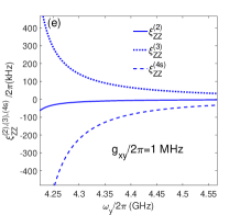
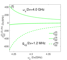
The is the second-order static ZZ coupling between two qubits, and describes the third-order static ZZ coupling between two qubits intermediated by the resonator . We use to label fourth-order static ZZ coupling contributed by the self-kerr resonance intermediated by the resonator , and the describe the static ZZ coupling induced by the cross-kerr resonance.
Even being listed together, the second-order , third-order , and fourth-order (self-kerr) static ZZ coupling terms come from different sources. As shown in Eqs.(16) and (17), the second-order term originates from the direct qubit-qubit coupling [6, 7, 8, 17], and the fourth-order term results from the perturbation expansion of qubit-resonator dispersive coupling[39, 41], while the third-order term is joint effects of direct qubit-qubit coupling and qubit-resonator interaction. Here describes the nonlinearity of resonator induced by the qubit-resonator dispersive coupling[40]. Since , the contributions of direct qubit-qubit and resonator-resonator couplings to fourth-order static ZZ coupling are neglected.
IV.2 Suppression of the Static ZZ coupling
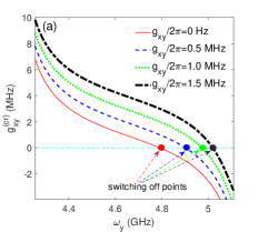
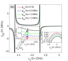
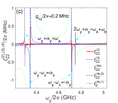
In this section, we try to suppress the Static ZZ coupling with the direct qubit-qubit coupling which can be arbitrary small in the double-coupler superconducting circuit. By setting GHz, the curves of static ZZ coupling are plotted in Fig. 6(b) according to Eqs.(16)-(18). The four curves correspond to different direct qubit-qubit coupling strengths. In the regimes suitable for the two-qubit gates, the values of static ZZ coupling are apparently suppressed by the weaker direct qubit-qubit coupling as shown in the insert figure. And the values of and are obviously suppressed by weaker direct qubit-qubit coupling in Fig. 6(c) ( MHz) compared with the results in Fig. 6(d) ( MHz). As shown in Fig. 6(b)-6(f), the static ZZ coupling can be suppressed below Sub-MHz in double-resonator coupler circuit, which is the similar level with transmon-based coupler circuit[7, 16].
For each static ZZ coupling curve in Fig. 6(b), two poles appear at and which originate from resonant state exchanges between the state and , respectively. There is also a pole locating at in each curve of static ZZ coupling in Fig. 6(b), and the poles also appears in the dashed curves (third-order static ZZ coupling) and dotted curve (fourth-order self-kerr resonance static ZZ coupling) in Figs. 6(c) and 6(d), so it should originate the qubit-qubit resonance state exchanges as indicated by the term containing in Eqs.(17)-(18). As shown in Fig. 6(a), the switching off positions in double-resonator couplers circuit can be below 5 GHz which is very close to the regimes of two-qubit gate. If the frequency of qubit y is tuned away from the switching off positions, the effective qubit-qubit coupling quickly increase to above 5 MHz for the two-qubit gates.
IV.3 Cancellation of the Static ZZ coupling
The nonzero residual coupling leads to unnecessary always-on quantum gates and additional accumulated phases, which are the dominant obstructions for the further enhancement of two-qubit gate fidelities. Recently, some work announce to eliminate the static ZZ coupling in the superconducting quantum chip[25, 35, 36], and it might also be removed in our proposed scheme through the destructive interferences of double-path couplers.
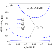
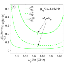
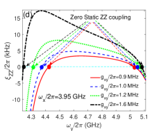
When we tune frequencies of qubit x to satisfy , and then the static ZZ coupling can be zeroes at some points as shown in Figs. 7(b) and 7(d), thus the static ZZ coupling are eliminated in the double-resonator coupler circuit. The signs of second-order , third-order and fourth-order (self-kerr resonance) static ZZ coupling are different in Figs. 7(e) and 7(f), and they cancel each other and eliminate the static ZZ coupling at certain points. It should be mentioned that the pole at in Figs. 6 do not appear in Figs. 7(b) just because they are outside the scope of drawing.
As shown in Fig. 7(a) (or Fig. 7(c)) and Fig.7(b) (or Fig. 7(d)), the static ZZ coupling are not switched off together with the effective qubit-qubit coupling. This result is not difficult to understand for the perturbation calculation methods[25, 16], because the effective qubit-qubit coupling is calculated only up to the second-order dispersive interaction (ac-Stark/Lamb Shifts), but static ZZ coupling contains some the high-order effects, such as self-kerr resonance, cross-kerr resonance, the high-excited states corrections, and so on. The intervals between zero value positions of static ZZ coupling and effective qubit-qubit coupling change for different direct qubit-qubit coupling strengths, and the black-dash-dotted curves ( MHz) get the smallest interval in Figs. 7(a) and 7(b). When we set GHz, the blue-dashed curves ( MHz) get the smallest interval in Figs. 7(c) and 7(d). So the interval between the switching off and zero static ZZ coupling points can be tuned by the direct qubit-qubit coupling and the frequencies of qubits, and it is possible to conduct the switching off and two-qubit gates both at the Zero static ZZ coupling regimes in the double-coupler superconducting circuit.
IV.4 Corrections to Static ZZ coupling
If we incorporate the variations of nonlinear term during the decoupling processes of the qubit-resonator interactions, and then the cross-kerr resonances will contribute to the ZZ coupling[39, 40, 41]. The resonator couplers are not pumped by external fields, the average cavity photon number is much smaller than one, so the single virtual photon exchanges will dominate the cross-kerr resonance processes. The cross-kerr resonance terms and in Eq.(15) describe the physical processes of virtual photon exchange between a qubit and two resonators, we plot the energy-level diagrams of single-virtual photon exchange process of cross-kerr resonance for qubit x in Fig. 8. For simplicity, only three lowest energy levels of superconducting artificial atoms are considered. The virtual photon exchange processes of cross-kerr resonance for qubit y can be obtained by replacing the x with y in Fig. 8 .
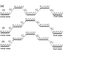
When qubit x is initially in the ground states, the Energy-level diagrams of cross-kerr resonance among qubit x, resonator a, and resonator b are shown in Fig. 8(a). The six cross-kerr resonances are attributed as three types of virtual photon exchange processes among qubit x, resonator a, and resonator b [39]. The first type: the qubit x absorbs a virtual photon from resonator a (or b) and transits to the first-excited states from the ground state, and it immediately returns the virtual photon to resonator a (or b) and decays to the ground state. Subsequently the qubit x jumps to the first-excited state again by getting another virtual photon from resonator b (or a), and finally it emits the virtual photon to resonator b (or a) and decays to the ground state. The second type: the qubit x transits to the first-excited state from the ground state by absorbing a virtual photon from resonator a (or b) and immediately jumps to the second-excited state by taking another virtual photon from resonator b (or a). Subsequently the qubit jumps to the first-excited state by emitting a virtual photon to the resonator b (or a), and finally decays to the ground state by emitting another virtual photon to resonator a (or b). The third type: the first two transition processes are the same as the second type, but the qubit firstly returns a virtual photon to resonator a (or b) in the third transition process and transits to the first-excited state, and finally decays to the ground state by emitting another photon to resonator b (or a). The virtual photon exchange processes for cross-kerr resonances among qubit y, resonator a, and resonator b can be obtained by replacing the qubit x with qubit y in Fig. 8(a). Adding together the contributions of the six type cross-kerr resonant processes, and we can obtain the energy level corrections to the ground state of qubit [39],
| (19) | |||
For simplicity, we have neglected the small differences on the interactions of a resonator with different energy levels of superconducting artificial atom, that is .
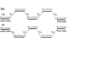
When the qubit x is the initially in the first-excited state, the Energy-level diagrams of cross-kerr resonance among qubit x, resonator a, and resonator b are shown in Fig. 8(b). The four cross-kerr resonances are attributed as two types of virtual photon exchange processes. The first type: the qubit x in the first-excited state absorbs a virtual photon from resonator a (or b) and transits to the second-excited state, and it immediately returns the photon to resonator a (or b) and jumps to the first-excited state. Subsequently the qubit jumps to the second-excited state again by getting another virtual photon from resonator b (or a) and finally it emits the photon to resonator b (or a) and jumps to the first-excited state. The second type: the qubit (in the first-excited state) emits a virtual photon to resonator a (or b) and decays to the ground state and immediately transits to the first-excited state by absorbing a virtual photon from resonator a (or b). Subsequently the qubit emits a virtual photon to resonator b (or a) and decays to the ground state and immediately absorbs another virtual photon from resonator b (or a) and finally jumps to the first-excited state. The virtual photon exchange processes for cross-kerr resonances among qubit y, resonator a, and resonator b can be obtained by replacing the qubit x with qubit y in Fig. 8(b). Adding together the contributions of the four type cross-kerr resonant processes, and we can obtain the energy level corrections to the first-excited state of qubit [39],
| (20) | |||||
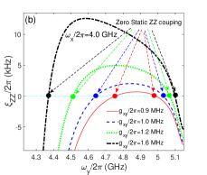
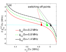
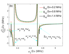
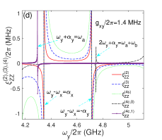
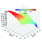
Adding the corrections by the cross-kerr resonances, the total ZZ coupling can be defined as , with , , , and . We plot the second-order (red-solid curves), third-order (blue-dashed curves), and fourth-order (self-kerr resonance) (green-dotted curves) static ZZ coupling in Fig. 9(c) ( MHz) and Fig. 9(d) ( MHz). By reducing the direct qubit-qubit coupling strengths, the values of static ZZ coupling curves are apparently suppressed in Fig. 9(c) ( MHz) compared with the result in Fig. 9(d) ( MHz). The energy level corrections to qubit’s ground state () and first-excited state () by the cross-kerr resonances are respectively plotted in the black dashed-dot curves and marked purple-solid curves in Figs. 9(c) and 9(d).
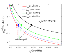
The curves of effective qubit-qubit coupling are plotted in Fig. 9(a), and values of direct qubit-qubit coupling affect switching off positions. Similar with Fig. 6(b), the two poles locating at and also appear in each curve of static ZZ coupling in Fig. 9(b). But there are two new poles in each curve of static ZZ coupling in Fig. 9(b) which should originate from the cross-kerr resonance[39, 40]. As indicated by Eqs.(19) and (20), the cross-kerr resonances through virtual photon exchanges induces additional poles for the static ZZ coupling at the point: (from Eq.(19)), (from Eq.(20)), and (from Eq.(20)). So we can see two new poles at and in each curve of Fig. 9(b). Another pole () is out of the scope of the drawing. As shown in Figs. 9(c) and 9(d), the pole at only appears on the black dash-dotted curves which correspond to the level correction to qubits’ ground states by the cross-kerr resonance . While the pole at only appears in the marked purple-solid curve which describes the level correction to qubits’ first-excited states by the cross-kerr resonance . In this article, we neglect the level corrections of cross-kerr resonances to the double-excited state , which should correspond to more complex physical processes.
V Conclusions
In conclusion, we have studied the mechanism of the switching off in the superconducting circuit consisting of two fixed-frequency resonator couplers. The induced indirect qubit-qubit coupling by two resonators can be cancelled, so the switching off can be realized without the direct qubit-qubit coupling. The frequencies of couplers can be much smaller than the single transmon-based coupler circuit, and this leaves wider available frequency spaces for couplers (or qubits), thus the frequency crowding on the superconducting chip might be relieved.
The weak direct qubit-qubit coupling can be used to suppress the static ZZ coupling in the double-coupler circuit, and the destructive interferences between double-path couplers can eliminate the static ZZ coupling, thus the quality of superconducting quantum chip might be enhanced. Our proposed double-resonator couplers scheme can unfreeze some restrictions on the superconducting quantum chip, mitigate the static ZZ coupling, and also save the dilution refrigerator lines, which might be a promising platform for superconducting quantum chip.
VI ACKNOWLEDGMENTS
H.W. is supported by the Natural Science Foundation of Shandong Province under Grant No. ZR2023LZH002 and the Inspur artificial intelligence research institute. Y.J.Z. is supported by Beijing Natural Science Foundation under Grant No. 4222064 and NSFC under Grant No. 11904013. X.-W.X. is supported by the National Natural Science Foundation of China under Grant No. 12064010, and Natural Science Foundation of Hunan Province of China under Grant No. 2021JJ20036.
Appendix A: The numerical calculation of the energy levels

In this section, we use the numerical method to calculate the two-dimensional energy level curved surfaces of the double-resonator couplers circuit (Fig. 1). Since the anharmonicities of Xmon qubit is very small, we regard the superconducting artificial atom as a multi-energy levels system in this section[39, 16]. The Hamiltonian for the circuit in Fig. 1 can be written as
where , and they respectively label the -th, -th, -th, and -th quantum states of qubit , with and . Between the quantum states and , we define the angular momentum operators as . The ladder operators can be introduced by and , thus we can get , , and . The corresponding transition frequency between states and is defined as , the describe the corresponding coupling strengths with resonator coupler . The describes the direct coupling strengths between the transition processes of for qubits x and for qubit y.
With the QuTiP software, we calculate the two-dimensional curved surfaces for the energy level of single-excited (Figs. 10(a)-10(d)) and double-excited (Figs. 10(e)-10(s)) states. During the numerical calculations with the QuTiP software, we truncate to the second excited states of qubits and assume and . Because of the anti-crossing effects, each curved surface in Fig. 10 can not describe a total energy level of certain quantum state, and we label the Z-axis of each figure by the corresponding state at zero magnetic flux.
Appendix B: Circuit Quantization
In this section, we conduct the quantization for the superconducting circuit in Fig. 1. The kinetic energy of the superconducting circuit can be obtained as [17, 20]
| (B.1) | |||||
As indicated by Fig. 1(b), the self-capacitances of the qubits and resonators is , and the relative capacitance between arbitrary two devices is defined as ( ), here with . Here and are the respective magnetic fluxes of the circuit nodes of resonators a and b, while and are respective node fluxes of qubits x and y. If we define the vector , thus the kinetic energy in Eq.(B.1) can be written as , with
| (B.6) |
where we have defined the coefficients: , , , and .
The potential energy for the superconducting circuit can be written as
| (B.7) | |||||
where is the Josephson energy of qubit , is the corresponding critical current, and is the flux quantum.
The Lagrangian of the superconducting circuit can be obtained by the definition , thus the generalized momentum can be defined as (), and it can be written in the vector form as . Thus the Hamiltonian of superconducting circuit can be written as , the inverse matrix is defined as
| (B.12) |
where is the adjugate matrix of . With the conditions , thus , we get approximate expressions for the elements in as
| (B.13) | |||||
Thus the Hamiltonian of double-resonator couplers circuit can be expressed as
The two-body coupling strengths can be defined as
| (B.15) | |||||
| (B.16) | |||||
| (B.17) |
The qubit-resonator interaction terms in Eq.(B.9) could induce indirect coupling between two qubits, which should be decoupled to obtained the effective qubit-qubit coupling.
Appendix C: Decoupling processes
The Josephson energy of Xmon qubit is much larger than its capacitance energy, , and then we can approximately get . If we introduce the creation and annihilation operators by the definitions: and , then second-quantized Hamiltonian can be obtained as , with
| (C.1) | |||||
| (C.2) | |||||
| (C.3) | |||||
| (C.4) | |||||
| (C.5) |
The transition frequencies of resonators and qubits are respectively defined as and , while the describe the anharmonicity of qubit .
In the qubit-resonator dispersive coupling regimes, , we can use the Schrieffer-Wolf transformation to decouple the variables of qubits and resonators. Since the resonator couplers are not pumped by the external fields, and the average cavity photon number should be much smaller than one, so the virtual photon exchanges will dominate the cross-kerr resonances. We define . Under the Unitary transformation , if we choose , thus the decoupled Hamiltonian can be obtained as
| (C.6) | |||||
The rotating wave approximation has been used to derive the above formula, and the constant terms were neglected. We also neglected the effects of small quantities ( and ). The anharmonicities of qubits are considered as invariant during Unitary transformation ( ), so some high-order effects relating to high-excited states of superconducting artificial atoms are neglected.
The transition frequencies of qubits, the resonant frequencies of resonators, the qubit-qubit coupling strength, and the resonator-resonator coupling strength in decoupled coordinate are obtained as
| (C.7) | |||||
| (C.8) | |||||
| (C.9) | |||||
| (C.10) | |||||
The is the decoupled qubit-qubit coupling strength which can be used to analyze the switching off. The is the decoupled resonator-resonator and much smaller than the frequency detuning between two resonators (), thus its contributions are neglected in this article.
Appendix D:Calculations of High-energy level corrections
In the current theoretical model, the kerr-nonlinear terms term are assumed bo be invariant () during the derivations of Eqs.(C.6). This means that some high-order effects and the contributions of high excited state of superconducting artificial atom are neglected, so the decoupled frequency and effective qubit-qubit coupling in Eqs.(C.7)-(C.12) contain no information of qubits’ anharmoncities. But anharmoncity of Xmon qubit is very small, thus the resonator can couple to the high-excited states of atoms, which should affect the transition frequencies of qubits and the effective qubit-qubit coupling strengths. As discussed by some theoretical work, the anharmonicity could induced fourth-order self-kerr and cross-kerr resonances, these effects could create corrections to the qubit’s energy levels[40, 39].
Bogoliubov transformation is used to analyze the higher-order effect during the decoupling processes for the qubit-resonator interactions[40]. To maintain consistency, in this article we still use the Schrieffer-Wolf transformation to analyze the contributions of the kerr-nonlinear terms during the decoupling process. In the qubit-resonator dispersive coupling regimes, and , we define , here . Since is a small quantity, we can separately conduct the Unitary transform [40], thus we get
| (D.1) | |||||
The commutation relation for the first-order expansion term,
| (D.2) | |||||
Since , we have neglected the effects of the weak direct qubit-qubit and resonator-resonator interactions.
The commutation relation for the second-order expansion term,
| (D.3) | |||||
Up to the second-order expanding terms, keeping the energy and particle number conservation terms, we can get the nonlinear term for qubit in the decoupled coordinate as
| (D.4) | |||||
In the right side of Eq.(D.4), the first line describes the self-kerr resonance, while the second line labels to the cross-kerr resonance. The third line describe the double virtual processes between one qubit and one resonator. The fourth line describes combined physical processes that the qubit and the resonator exchange a virtual photon, and the qubit simulatively participates the self-excitation and subsequent self-annihilation processes.
References
- [1] A.P.M. Place, L.V.H. Rodgers, P. Mundada, B.M. Smitham, M. Fitzpatrick, Zhaoqi Leng, A. Premkumar, J. Bryon, A. Vrajitoarea, S. Sussman, Guangming Cheng, T. Madhavan, H.K. Babla, Xuan Hoang Le, Youqi Gang, B. Jäck, A. Gyenis, Nan Yao, R.J. Cava, N.P. de Leon, and A.A. Houck, New material platform for superconducting transmon qubits with coherence times exceeding 0.3 milliseconds, Nat. Commun. 12, 1779 (2021).
- [2] Chenlu Wang, Xuegang Li, Huikai Xu, Zhiyuan Li, Junhua Wang, Zhen Yang, Zhenyu Mi, Xuehui Liang, Tang Su, Chuhong Yang, Guangyue Wang, Wenyan Wang, Yongchao Li, Mo Chen, Chengyao Li, Kehuan Linghu, Jiaxiu Han, Yingshan Zhang, Yulong Feng, Yu Song, Teng Ma, Jingning Zhang, Ruixia Wang, Peng Zhao, Weiyang Liu, Guangming Xue, Yirong Jin, and Haifeng Yu, Towards practical quantum computers: transmon qubit with a lifetime approaching 0.5 milliseconds, npj Quantum Informat. 8, 3 (2022).
- [3] Wenhui Ren, Weikang Li, Shibo Xu, Ke Wang, Wenjie Jiang, Feitong Jin, Xuhao Zhu, Jiachen Chen, Zixuan Song, Pengfei Zhang, Hang Dong, Xu Zhang, Jinfeng Deng, Yu Gao, Chuanyu Zhang, Yaozu Wu, Bing Zhang, Qiujiang Guo, Hekang Li, Zhen Wang, Jacob Biamonte, Chao Song, Dong-Ling Deng, and H. Wang, Experimental quantum adversarial learning with programmable superconducting qubits, Nat. Comput. Sci. 2, 711 (2022).
- [4] Shibo Xu, Zheng-Zhi Sun, Ke Wang, Liang Xiang, Zehang Bao, Zitian Zhu, Fanhao Shen, Zixuan Song, Pengfei Zhang, Wenhui Ren, Xu Zhang, Hang Dong, Jinfeng Deng, Jiachen Chen, Yaozu Wu, Ziqi Tan, Yu Gao, Feitong Jin, Xuhao Zhu, Chuanyu Zhang, Ning Wang, Yiren Zou, Jiarun Zhong, Aosai Zhang, Weikang Li, Wenjie Jiang, Li-Wei Yu, Yunyan Yao, Zhen Wang, Hekang Li, Qiujiang Guo, Chao Song, H. Wang, Dong-Ling Deng, Digital simulation of non-Abelian anyons with 68 programmable superconducting qubits, Chin. Phys. Lett. 40 060301 (2023).
- [5] M. Bal, A.A. Murthy, Shaojiang Zhu, F. Crisa, Xinyuan You, Ziwen Huang, T. Roy, J. Lee, D. van Zanten, R. Pilipenko, I. Nekrashevich, D. Bafia, Y. Krasnikova, C. J. Kopas, E. O. Lachman, D. Miller, J. Y. Mutus, M.J. Reagor, H. Cansizoglu, J. Marshall, D.P. Pappas, Kim Vu, K. Yadavalli, Jin-Su Oh, Lin Zhou, M.J. Kramer, F.Q. Lecocq, D.P. Goronzy, C.G. Torres-Castanedo, G. Pritchard, V.P. Dravid, J.M. Rondinelli, M.J. Bedzyk, M.C. Hersam, J. Zasadzinski, J. Koch, J.A. Sauls, A. Romanenko, and A. Grassellino, Systematic Improvements in Transmon Qubit Coherence Enabled by Niobium Surface Encapsulation, https://arxiv.org/abs/2304.13257 (2023).
- [6] Y. Chen, C. Neill, P. Roushan, N. Leung, M. Fang, R. Barends, J. Kelly, B. Campbell, Z. Chen, B. Chiaro, A. Dunsworth, E. Jeffrey, A. Megrant, J. Y. Mutus, P. J. J. ÓMalley, C. M. Quintana, D. Sank, A. Vainsencher, J. Wenner, T. C. White, Michael R. Geller, A. N. Cleland, and J. M. Martinis, qubit Architecture with High Coherence and Fast Tunable Coupling, Phys. Rev. Lett. 113, 220502 (2014).
- [7] F. Yan, P. Krantz, Y. Sung, M. Kjaergaard, D. L. Campbell, T. P. Orlando, S. Gustavsson, and W. D. Oliver, Tunable Coupling Scheme for Implementing High-Fidelity Two-qubit Gates, Phys. Rev. Appl. 10, 054062 (2018).
- [8] X. Li, T. Cai, H. Yan, Z. Wang, X. Pan, Y. Ma, W. Cai, J. Han, Z. Hua, X. Han, Y. Wu, H. Zhang, H. Wang, Yipu Song, Luming Duan, and Luyan Sun, Tunable Coupler for Realizing a Controlled-Phase Gate with Dynamically Decoupled Regime in a Superconducting Circuit, Phys. Rev. Appl. 14, 024070 (2020).
- [9] Yuan Xu, Ji Chu, Jiahao Yuan, Jiawei Qiu, Yuxuan Zhou, Libo Zhang, Xinsheng Tan, Yang Yu, Song Liu, Jian Li, Fei Yan, and Dapeng Yu, High-Fidelity, High-Scalability Two-Qubit Gate Scheme for Superconducting Qubits, Phys. Rev. Lett. 125, 240503 (2020).
- [10] J. Stehlik, D.M. Zajac, D.L. Underwood, T. Phung, J. Blair, S. Carnevale, D. Klaus, G.A. Keefe, A. Carniol, M. Kumph, M. Steffen, and O.E. Dial, Tunable Coupling Architecture for Fixed-Frequency Transmon Superconducting Qubits, Phys. Rev. Lett. 127, 080505 (2021).
- [11] I.N. Moskalenko, I.A. Simakov, N.N. Abramov, A.A. Grigorev, D.O. Moskalev, A.A. Pishchimova, N.S. Smirnov, E.V. Zikiy, I.A. Rodionov, and I.S. Besedin, High fidelity two-qubit gates on fluxoniums using a tunable coupler, Npj Quantum Inform. 8, 130 (2022).
- [12] A. Kandala, K. X. Wei, S. Srinivasan, E. Magesan, S. Carnevale, G. A. Keefe, D. Klaus, O. Dial, and D. C. McKay, Demonstration of a High-Fidelity cnot Gate for Fixed-Frequency Transmons with Engineered ZZ Suppression, Phys. Rev. Lett. 127, 130501 (2021).
- [13] Qingling Zhu, Sirui Cao, Fusheng Chen, Ming-Cheng Chen, Xiawei Chen, Tung-Hsun Chung, Hui Deng, Yajie Du, Daojin Fan, Ming Gong, Cheng Guo, Chu Guo, Shaojun Guo, Lianchen Han, Linyin Hong, He-Liang Huang, Yong-Heng Huo, Liping Li, Na Li, Shaowei Li, Jian-Wei Pan, Quantum computational advantage via 60-qubit 24-cycle random circuit sampling, Sci. Bull. 67, 240 (2022).
- [14] F. Arute, K. Arya, R. Babbush, D. Bacon, J. C. Bardin, R. Barends, R. Biswas, S. Boixo, F. G. S. L. Brandao, D. A. Buell, B. Burkett, Yu Chen, Zijun Chen, B. Chiaro, R. Collins, W. Courtney, A. Dunsworth, E. Farhi, B. Foxen, A. Fowler, C. Gidney, M. Giustina, R. Graff, K. Guerin, S. Habegger, M. P. Harrigan, M. J. Hartmann, A. Ho, M. Hoffmann, T. Huang, T. S. Humble, S. V. Isakov, E. Jeffrey, Zhang Jiang, D. Kafri, K. Kechedzhi, Julian Kelly, P. V. Klimov, S. Knysh, A. Korotkov, F. Kostritsa, D. Landhuis, M. Lindmark, E. Lucero, D. Lyakh, S. Mandrà, J. R. McClean, M. McEwen, A. Megrant, Xiao Mi, K. Michielsen, M. Mohseni, J. Mutus, O. Naaman, M. Neeley, C. Neill, M. Y. Niu, E. Ostby, A. Petukhov, J. C. Platt, C. Quintana, E. G. Rieffel, P. Roushan, N. C. Rubin, D. Sank, K. J. Satzinger, V. Smelyanskiy, K. J. Sung, M. D. Trevithick, A. Vainsencher, B. Villalonga, T. White, Z. J. Yao, P. Yeh, A. Zalcman, H. Neven, J. M. Martinis, Quantum supremacy using a programmable superconducting processor, Nature 574, 505 (2019).
- [15] Yulin Wu, Wan-Su Bao, Sirui Cao, Fusheng Chen, Ming-Cheng Chen, Xiawei Chen, Tung-Hsun Chung, Hui Deng, Yajie Du, Daojin Fan, Ming Gong, Cheng Guo, Chu Guo, Shaojun Guo, Lianchen Han, Linyin Hong, He-Liang Huang, Yong-Heng Huo, Liping Li, Na Li, Shaowei Li, Yuan Li, Futian Liang, Chun Lin, Jin Lin, Haoran Qian, Dan Qiao, Hao Rong, Hong Su, Lihua Sun, Liangyuan Wang, Shiyu Wang, Dachao Wu, Yu Xu, Kai Yan, Weifeng Yang, Yang Yang, Yangsen Ye, Jianghan Yin, Chong Ying, Jiale Yu, Chen Zha, Cha Zhang, Haibin Zhang, Kaili Zhang, Yiming Zhang, Han Zhao, Youwei Zhao, Liang Zhou, Qingling Zhu, Chao-Yang Lu, Cheng-Zhi Peng, Xiaobo Zhu, and Jian-Wei Pan, Strong Quantum Computational Advantage Using a Superconducting Quantum Processor, Phys. Rev. Lett. 127, 180501 (2021).
- [16] Y. Sung, L. Ding, J. Braumüller, A. Vepsäläinen, B. Kannan, M. Kjaergaard, A. Greene, G. O. Samach, C. McNally, D. Kim, A. Melville, B. M. Niedzielski, M. E. Schwartz, J. L. Yoder, T. P. Orlando, S. Gustavsson, and W. D. Oliver, Realization of High-Fidelity CZ and ZZ-Free ISWAP Gates with a Tunable Coupler, Phys. Rev. X 11, 021058 (2021).
- [17] Hui Wang, Yan-Jun Zhao, Rui Wang, Xun-Wei Xu, Qiang Liu, Jianhua Wang, and Changxin Jin, Frequency Adjustable Resonator as a Tunable Coupler for Xmon Qubits, J. Phys. Soc. Jpn. 91, 104005 (2022).
- [18] Ming Gong, Shiyu Wang, Chen Zha, Ming-Cheng Chen, He-Liang Huang, Yulin Wu, Qingling Zhu, Youwei Zhao, Shaowei Li, Shaojun Guo, Haoran Qian, Yangsen Ye, Fusheng Chen, Chong Ying, Jiale Yu, Daojin Fan, Dachao Wu, Hong Su, Hui Deng, Hao Rong, Kaili Zhang, Sirui Cao, Jin Lin, Yu Xu, Lihua Sun, Cheng Guo, Na Li, Futian Liang, V. M. Bastidas, Kae Nemoto, W. J. Munro, Yong-Heng Huo, Chao-Yang Lu, Cheng-Zhi Peng, Xiaobo Zhu, Jian-Wei Pan, Quantum walks on a programmable two-dimensional 62-qubit superconducting processor, Science 372, 948(2021).
- [19] IBM-Q-Team, IBM-Q-53 Rochester backend specification v1.2.0, (2020).
- [20] Yulin Wu, Li-Ping Yang, Ming Gong, Yarui Zheng, Hui Deng, Zhiguang Yan, Yanjun Zhao, Keqiang Huang, A. D Castellano, W. J Munro, K. Nemoto, Dong-Ning Zheng, C.P. Sun, Yu-xi Liu, Xiaobo Zhu, Li Lu, An efficient and compact switch for quantum circuits, npj Quantum Inf. 4, 50 (2018).
- [21] J. Stehlik, D.M. Zajac, D.L. Underwood, T. Phung, J. Blair, S. Carnevale, D. Klaus, G.A. Keefe, A. Carniol, M. Kumph, M. Steffen, and O.E. Dial, Tunable Coupling Architecture for Fixed-Frequency Transmon Superconducting Qubits, Phys. Rev. Lett. 127, 080505 (2021).
- [22] D.C. McKay, S. Filipp, A. Mezzacapo, E. Magesan, J.M. Chow, and J.M. Gambetta, Universal Gate for Fixed-Frequency Qubits via a Tunable Bus, Phys. Rev. Appl. 6, 064007(2016).
- [23] P. Mundada, Gengyan Zhang, T. Hazard, and A. Houck, Suppression of Qubit Crosstalk in a Tunable Coupling Superconducting Circuit, Phys. Rev. Appl. 12, 054023 (2019).
- [24] Hayato Goto, Double-Transmon Coupler: Fast Two-Qubit Gate with No Residual Coupling for Highly Detuned Superconducting Qubits, Phys. Rev. Appl. 18, 034038 (2022).
- [25] E. A. Sete, A. Q. Chen, R. Manenti, S. Kulshreshtha, and S. Poletto, Floating Tunable Coupler for Scalable Quantum Computing Architectures, Phys. Rev. Appl. 15, 064063 (2021).
- [26] J. R. Johansson, P. D. Nation, and F. Nori: ”QuTiP 2: A Python framework for the dynamics of open quantum systems.”, Comp. Phys. Comm. 184, 1234 (2013) [DOI: 10.1016/j.cpc.2012.11.019].
- [27] J. R. Johansson, P. D. Nation, and F. Nori: ”QuTiP: An open-source Python framework for the dynamics of open quantum systems.”, Comp. Phys. Comm. 183, 1760 (2012) [DOI: 10.1016/j.cpc.2012.02.021].
- [28] Huichen Sun, Tunable Coupler in Superconducting Circuits and Impedance Engineering for Josephson Parametric Amplifier. MS thesis. University of Waterloo (2020).
- [29] N.J. Glaser, F. Roy, and S. Filipp, Controlled-Controlled-Phase Gates for Superconducting Qubits Mediated by a Shared Tunable Coupler, Phys. Rev. Appl. 19, 044001 (2023).
- [30] Mi. H. Devoret, Quantum fluctuations in electrical circuits, Les Houches, Session LXIII 7 (1995).
- [31] S. M. Girvin, Circuit qed: Superconducting qubits coupled to microwave photons, Proceedings of the 2011 Les Houches Summer School (2011).
- [32] P. Mundada, Gengyan Zhang, T. Hazard, and A. Houck, Suppression of Qubit Crosstalk in a Tunable Coupling Superconducting Circuit, Phys. Rev. Appl.12, 054023 (2019).
- [33] Peng Zhao, Kehuan Linghu, Zhiyuan Li, Peng Xu, Ruixia Wang, Guangming Xue, Yirong Jin, and Haifeng Yu, Quantum Crosstalk Analysis for Simultaneous Gate Operations on Superconducting Qubits PRX Quantum 3, 020301 (2022).
- [34] A.C. Santos, Role of parasitic interactions and microwave crosstalk in dispersive control of two superconducting artificial atoms, Phys. Rev. A 107, 012602 (2023).
- [35] Peng Zhao, Peng Xu, Dong Lan, Ji Chu, Xinsheng Tan, Haifeng Yu, and Yang Yu, High-Contrast ZZ Interaction Using Superconducting Qubits with Opposite-Sign Anharmonicity Phys. Rev. Lett. 125, 200503 (2020).
- [36] Jaseung Ku, Xuexin Xu, Markus Brink, David C. McKay, Jared B. Hertzberg, M.H. Ansari, and B.L.T. Plourde, Suppression of Unwanted ZZ Interactions in a Hybrid Two-Qubit System Phys. Rev. Lett. 125, 200504 (2020).
- [37] F. Marxer, A. Vepsäläinen, S. W. Jolin, J. Tuorila, A. Landra, C. Ockeloen-Korppi, Wei Liu, O. Ahonen, A. Auer, L. Belzane, V. Bergholm, Chun Fai Chan, Kok Wai Chan, T. Hiltunen, J. Hotari, E. Hyyppä, J. Ikonen, D. Janzso, M. Koistinen, J. Kotilahti, Tianyi Li, J. Luus, M. Papic, M. Partanen, J. Räbinä, J. Rosti, M. Savytskyi, M. Seppälä, V. Sevriuk, E. Takala, B. Tarasinski, M. J. Thapa,. F. Tosto, N. Vorobeva, Liuqi Yu, Kuan Yen Tan, Juha Hassel, M. Möttönen, and J. Heinsoo, Long-Distance Transmon Coupler with cz-Gate Fidelity above , PRX Quantum 4, 010314 (2023).
- [38] C. Leroux, A. D. Paolo, and A. Blais, Superconducting coupler with exponentially large on-off ratio, Phys. Rev. Appl. 16, 064062 (2021).
- [39] Guanyu Zhu, D. G. Ferguson, V. E. Manucharyan, and J. Koch, Circuit QED with fluxonium qubits: Theory of the dispersive regime, Phys. Rev. B 87, 024510 (2013).
- [40] A. Blais, A.L. Grimsmo, S.M. Girvin, and A. Wallraff, Circuit quantum electrodynamics, Rev. Mod. Phys. 93, 025005 (2021).
- [41] R. Krishnan and J. A. Pople, Approximate fourth-order perturbation theory of the electron correlation energy, Int. J. Quantum Chem.14, 91 (1978).