Topological Guided Actor-Critic Modular Learning of Continuous Systems with Temporal Objectives

Abstract

This work investigates the formal policy synthesis of continuous-state stochastic dynamic systems given high-level specifications in linear temporal logic. To learn an optimal policy that maximizes the satisfaction probability, we take a product between a dynamic system and the translated automaton to construct a product system on which we solve an optimal planning problem. Since this product system has a hybrid product state space that results in reward sparsity, we introduce a generalized optimal backup order, in reverse to the topological order, to guide the value backups and accelerate the learning process. We provide the optimality proof for using the generalized optimal backup order in this optimal planning problem. Further, this paper presents an actor-critic reinforcement learning algorithm when topological order applies. This algorithm leverages advanced mathematical techniques and enjoys the property of hyperparameter self-tuning. We provide proof of the optimality and convergence of our proposed reinforcement learning algorithm. We use neural networks to approximate the value function and policy function for hybrid product state space. Furthermore, we observe that assigning integer numbers to automaton states can rank the value or policy function approximated by neural networks. To break the ordinal relationship, we use an individual neural network for each automaton state’s value (policy) function, termed modular learning. We conduct two experiments. First, to show the efficacy of our reinforcement learning algorithm, we compare it with baselines on a classic control task, CartPole. Second, we demonstrate the empirical performance of our formal policy synthesis framework on motion planning of a Dubins car with a temporal specification.

I Introduction

Recently, formal policy synthesis has attracted substantial research attention because the synthesized policy can provide a provable satisfaction probabilistic guarantee for high-level specifications. High-level specifications can define more sophisticated system behaviors, distinguished from a traditional A-to-B motion planning task. For instance, a high-level specification can describe an autonomous taxi task: a taxi running out of gas/electricity needs to avoid the crowded downtown and complete: (a) visit a gas station and then drop the passenger at the destination or (b) drop the passenger then go to a gas station. Providing probabilistic guarantees brings significant values in a broad range of safety-critical applications, including robotics [1], military defense [2], cybersecurity [3], and other cyber-psychical systems [4]. One most encountered safety-critical example in robotics is that a robot avoids obstacles. If we can quantitatively evaluate the probability of a robot running into obstacles, we can trade off between this probability and other decisive factors, such as cost. Despite the theoretical successes and state-of-art experimental results on formal policy synthesis, there are challenges when implemented in real-world applications: (1) availability of system models; i.e., the system model is often unknown. (2) power of handling the continuous-state space; i.e., we encounter continuous systems almost all the time, while most published results are demonstrated on discrete systems.

This paper investigates the formal policy synthesis for continuous-state stochastic dynamic systems with high-level specifications expressed in linear temporal logic (LTL). LTL can succinctly specify a collection of desired system properties, such as safety, liveness, persistence, and stability [5]. To learn an optimal policy that maximizes the probability of satisfying a LTL formula, we follow an automaton-based approach. We take a product between the stochastic system and the task automaton, where we translate the task automaton via existing LTL-automaton conversion [6]. When the system visits the final states, it satisfies the specification and receives positive rewards; However, since this system has a hybrid state space, entering the final states requires extremely high sampling complexity, raising the sparse reward issue. To mitigate this issue, we generalize the optimal backup order in Markov decision process (MDP) to that in product MDP, in reverse to topological order, to guide the value backups and help accelerate the learning process. Topological order provides the structural information on the order of updating values of product states. We present an algorithm to update values level-by-level, where topological order introduces a set of level sets. Specifically, the system receives reward signals when it transits from the current level to the previous level whose values have converged and been optimal. We provide proof that using topological order still guarantees optimality.

Further, we propose a reinforcement learning (RL) algorithm where topological order applies. This algorithm only requires paths of the stochastic process but not the system model. Our proposed RL algorithm is a variant of the actor-critic algorithm and differs from the soft actor-critic (SAC) algorithm by the distinctive way of policy evaluation. We evaluate our policy by solving a sequential optimization problem and leveraging the augmented Lagrangian method for hyperparameter self-tuning. The proposed SAC algorithm alternates between: (a) policy evaluation and (b) policy improvement. We prove that our algorithm achieves optimality and convergence in a tabular case. We approximate value and policy functions for hybrid product state space by neural networks. However, by assigning integers to denote automaton states, it ranks values of different automaton states by integers [7]. Instead, we approximate each automaton state’s value (policy) functions by individual neural networks, termed modular learning. Specifically, if there are $N$ automaton states at the current level, we use $2N$ neural networks to approximate values and policy functions.

Compared to minimizing the temporal error like temporal difference learning [8], our policy evaluation is inspired by the linear programming solution for MDP [9]. By using the mellowmax operator, we formulate a similar constrained optimization problem. However, as the system is continuous/hybrid, we transform the original constrained optimization problem into an equivalent stochastic constrained optimization, and we only require the constraints to be satisfied on trajectories sampled in an off-policy manner. Further, to remove the system model in constraints, we adopt an unbiased estimate to approximate the value of the current state by using only the current action, the next state, and the reward of execution for the trajectories. We transform the inequality constraints into equality constraints by adopting the augmented Lagrangian method. We present an algorithm to solve this unconstrained optimization problem sequentially, where sequential solving means solving a sequence of subproblems with a fixed set of hyperparameters. At the end of each subproblem, we update the hyperparameters. The sequential optimization improves the value and policy function as the number of subproblems solved increases.

Contribution

Our central theoretical contribution is to present a comprehensive, efficient formal policy synthesis framework for continuous-state stochastic dynamic systems with high-level specifications. Learning a control policy that maximizes the satisfaction probability of high-level specifications is genuinely intractable when the system model is continuous and not available. We first introduce the topological order and define a generalized optimal backup order to mitigate reward sparsity in continuous/hybrid state space. We next present a sequential, actor-critic RL algorithm that only requires sampled trajectories by interacting with the environment. The algorithm converges and achieves optimality in a tabular case. Using neural networks is the standard practice to save the trouble of storing values/policies in continuous/hybrid space. But we approximate each value/policy function at each task state by one neural network to break the ordinal relationship between automaton states denoted by integers. We illustrate the empirical performance benefited from advanced mathematical methods by comparing our proposed RL algorithm with baselines. Further, we demonstrate the efficacy of our formal policy synthesis framework on motion planning of a Dubins car with a temporal specification.

II Preliminary

Notation

Let $\mathbb{R}$ denote the set of real numbers. For a set $X$, $2^{X}$ denotes its power set. We use the notation $\Sigma$ to denote a finite set of symbols, also known as the alphabet. A sequence of symbols $w=\sigma_{0}\sigma_{1}\dots\sigma_{n}$ with $\sigma_{i}\in\Sigma$ for any $0\leq i\leq n$ is called a finite word. The set $\Sigma^{\ast}$ is the set of all finite words. We denote the set of all $\omega$-regular words as $\Sigma^{\omega}$ obtained by concatenating the elements in $\Sigma$ infinitely many times. The indicator function is denoted by $\mathbf{1}$, where $\mathbf{1}(E)$ evaluates to be $1$ if the event $E$ is true, $0$ otherwise.

II-A Linear Temporal Logic and Labeled MDP

We use linear temporal Llogic (LTL) to describe a complex high-level task. An LTL is defined inductively as follows:

$$\varphi\coloneqq\top\mid p\mid\neg\varphi\mid\varphi_{1}\land\varphi_{2}\mid\bigcirc\,\varphi\mid\varphi_{1}{\mbox{$\,{\sf U}\,$}}\varphi_{2},$$

where $\top$ is universally true, and $p\in\mathcal{AP}$ is an atomic proposition. The operator $\bigcirc\,$ is a temporal operator called the “next” operator. The formula $\bigcirc\,\varphi$ means that the formula $\varphi$ will be true at the next state. The operator $\,{\sf U}\,$ is a temporal operator called the “until” operator. The formula $\varphi_{1}\mbox{$\,{\sf U}\,$}\varphi_{2}$ means that $\varphi_{2}$ will become true in some future time steps, and before that $\varphi_{1}$ holds true for every time step.

The operators $\Diamond\,$ (read as eventually) and $\Box\,$ (read as always) are defined using the operator $\,{\sf U}\,$ as follows: $\Diamond\,\varphi=\top\mbox{$\,{\sf U}\,$}\varphi$ and $\Box\,\varphi=\neg\Diamond\,\neg\varphi$. Given an $\omega$-regular word $w=\sigma_{0}\sigma_{1}\ldots\in(2^{\mathcal{AP}})^{\omega}$, $w\models\varphi$ holds if the following holds.

$$w \models\top$$

$$w \models p p\in\sigma_{0}(\text{i.e., }\sigma_{0}\models p),$$ iff

$$w \models\varphi_{1}\land\varphi_{2} w\models\varphi_{1}\land w\models\varphi_{2},$$ iff

$$w \models\neg\varphi w\not\models\varphi,$$ iff

$$w \models\bigcirc\,\varphi \sigma_{1}\sigma_{2}\sigma_{3}\ldots\models\varphi,$$ iff

$$w \models\varphi_{1}\mbox{$\,{\sf U}\,$}\varphi_{2} \exists j\geq 0,\sigma_{j}\sigma_{j+1}\ldots\models\varphi_{2},$$ iff

$$\text{ and }\sigma_{i}\sigma_{i+1}\ldots\models\varphi_{1},$$

$$\text{ for all }0\leq i<j.$$

For details about the syntax and semantics of LTL, the readers are referred to [10].

In this paper, we restrict the specifications to the class of syntactically co-safe LTL (scLTL) [11]. An scLTL formula contains only temporal operators $\Diamond\,$, $\bigcirc\,$, and $\,{\sf U}\,$ when written in a positive normal form [12] (i.e., the negation operator $\neg$ appears only in front of atomic propositions). The unique property of scLTL formulas is that a word satisfying an scLTL formula $\varphi$ only needs a good prefix. That is, given a good prefix $w\in\Sigma^{\ast}$, the word $ww^{\prime}\models\varphi$ satisfies the scLTL formula $\varphi$ for any $w^{\prime}\in\Sigma^{\omega}$. The set of good prefixes can be compactly represented as the language accepted by a deterministic finite-state automaton (DFA) defined as follows.

Definition 1 (Deterministic Finite-state Automaton (DFA)).

A DFA of an scLTL formula $\varphi$ is a tuple $\mathcal{A}=\langle Q,\Sigma,\delta,\iota,F\rangle$ that includes a finite set $Q$ of states, a finite set $\Sigma=2^{\mathcal{AP}}$ of symbols, a deterministic function $\delta\colon Q\times\Sigma\to Q$, a unique initial state $\iota$, and a set $F$ of accepting states.

For a finite word $w=\sigma_{0}\sigma_{1}\ldots\sigma_{n}\in\Sigma^{\ast}$, the DFA generates a sequence of states $q_{0}q_{1}\ldots q_{n+1}$ such that $q_{0}=\iota$ and $q_{i+1}=\delta(q_{i},\sigma_{i})$ for any $0\leq i\leq n$. The word $w$ is accepted by the DFA if and only if $q_{n+1}\in F$. The set of words accepted by the DFA $\mathcal{A}$ is called its language. We assume that the DFA is complete — that is, for every state-action pair $(q,\sigma)$, $\delta(q,\sigma)$ is defined. An incomplete DFA can be made complete by adding a sink state $q_{\mathsf{sink}}$ such that $\forall\sigma\in\Sigma,\delta(q_{\mathsf{sink}},\sigma)=q_{\mathsf{sink}}$, and directing all undefined transitions to the sink state $q_{\mathsf{sink}}$.

Example 1.

Figure 1: DFA accepting the formula $\varphi$.

A sequential visiting task requires a car to avoid obstacles and accomplish one of the following: (a) visit $A$ and do not visit $D$ or obstacles until $C$ is visited; (b) visit $D$ and do not visit $A$ or obstacles until $B$ is visited. To describe this task, we define a set $\mathcal{AP}$ of atomic propositions as follows:

• $A$: car reaches $A$.

• $B$: car reaches $B$.

• $C$: car reaches $C$.

• $D$: car reaches $D$.

• $O$: car reaches obstacles.

Given the set $\mathcal{AP}$ of atomic propositions, we can capture the sequential visiting task by an scLTL formula as follows:

$$\varphi=\neg O\mbox{$\,{\sf U}\,$}(\varphi_{1}\lor\varphi_{2}),$$

where

$$\varphi_{1}=(A\land((\neg D\land\neg O)\mbox{$\,{\sf U}\,$}C)),$$

$$\varphi_{2}=(D\land((\neg A\land\neg O)\mbox{$\,{\sf U}\,$}B)),$$

and the corresponding DFA is depicted in Fig. 1. For clarity, we trim self loops in Fig. 1. That is, for state $q_{0}$, we remove transitions from $q_{0}$ to $q_{0}$ via symbol $\sigma$, where $\sigma\in 2^{\mathcal{AP}}\setminus(\{A\}\cup\{D\})$. We remove transitions for state $q_{1},q_{2},q_{3}$, and $q_{4}$ similarly.

We consider a class of planning in stochastic systems subject to high-level specifications. A stochastic dynamic system can be modeled as a labeled Markov decision process (MDP).

Definition 2 (Labeled Markov Decision Process (MDP) [13]).

A labeled Markov decision process is a tuple

$$\operatorname{M}=\langle S,A,P,s_{0},L,\mathcal{AP}\rangle,$$

where the components of $\operatorname{M}$ are defined as follows:

• $S$ is a set of states.

• $A$ is a set of actions.

• $P\colon S\times A\times S\to[0,1]$ is the transition probability function, where $P(\cdot\mid s,a)$ represents the probability distribution over next states given an action $a\in A$ taken at the current state $s\in S$.

• $s_{0}$ is a unique initial state.

• $\mathcal{AP}$ is a set of atomic propositions.

• $L\colon S\to 2^{\mathcal{AP}}$ is the labeling function that maps a state $s\in S$ to a subset of propositions $L(s)\subseteq\mathcal{AP}$ that hold true at state $s$.

A randomized policy is a function $\pi\colon S\times A\to[0,1]$ maps the current state into a distribution over actions. The set of policies is denoted by $\Pi$. Given an MDP $\operatorname{M}$ and a policy $\pi$, the policy induces a distribution over state-action sequences, termed as paths. An infinite (resp. finite) path $\rho^{\pi}=s_{0}a_{0}s_{1}a_{1}\ldots\in(S\times A)^{\omega}$ (resp. $s_{0}a_{0}s_{1}a_{1}\ldots s_{N}\in(S\times A)^{\ast}S$) conditional on the policy $\pi$ being followed satisfies: for all $t\geq 0$, we have $s_{t+1}\sim P(\cdot\mid s_{t},a_{t})$ and $a_{t}\sim\pi(\cdot\mid s_{t})$. We denote the set of all paths as $\mathsf{path}$, the set of paths following policy $\pi$ as $\mathsf{path}^{\pi}$, and the set of paths starting at state $s$ as $\mathsf{path}(s)$. We use $\mathcal{D}^{\pi}$ to denote the trajectory distribution induced by the policy $\pi$ and $\mathcal{D}^{\pi}(s)$ to denote the trajectory distribution induced by the policy $\pi$ starting at state $s$.

Given a finite path $\rho=s_{0}a_{0}s_{1}a_{1}\dots s_{N}\in\mathsf{path}$, we obtain a sequence of labels $L(\rho)=L(s_{0})L(s_{1})\ldots L(s_{N})\in\Sigma^{\ast}$. A finite path $\rho$ satisfies the formula $\varphi$, denoted by $\rho\models\varphi$, if and only if $L(\rho)$ is accepted by the corresponding DFA.

II-B Problem Formulation

We aim to solve a MaxProb problem defined as follows.

Problem 1 (MaxProb Problem).

Given an MDP and a high-level specification expressed in an scLTL formula $\varphi$, the MaxProb is to learn an optimal policy $\pi^{\ast}$ that maximizes the probability of satisfying the formula $\varphi$. Formally,

$$\pi^{\ast}=\mathop{\mathrm{argmax}}_{\pi\in\Pi}\mathop{\bf E{}}\nolimits_{\rho_{t}\sim\mathcal{D}^{\pi}}[\sum_{t=0}^{\infty}\mathbf{1}(\rho_{t}\models\varphi)],$$ (1)

where $\rho_{t}=s_{0}a_{0}s_{1}a_{1}\dots s_{t}\in\mathsf{path}^{\pi}$.

III Automaton-based Formal Policy Synthesis

We introduce the product MDP to model the stochastic dynamic system with a high-level specification in scLTL.

Definition 3 (Product MDP).

Given a labeled MDP $\operatorname{M}=\langle S,A,P,s_{0},L,\mathcal{AP}\rangle$ and a DFA $\mathcal{A}=\langle Q,\Sigma,\delta,\iota,F\rangle$ associated with an scLTL formula $\varphi$, a product MDP is a tuple

$$\operatorname{\mathcal{M}}=\operatorname{M}\otimes\mathcal{A}=\langle Z,A,\operatorname{\Delta},z_{0},\operatorname{\mathcal{F}}\rangle,$$

where the components of $\operatorname{\mathcal{M}}$ are defined as follows:

• $Z\colon S\times Q$ is a set of product states. Every product state $z=(s,q)\in Z$ has two components:

  • $s$ is a state in MDP.

  • $q$ is an automaton state keeping track of the progress towards satisfying the specification.

• $A$ is a set of actions inherited from MDP.

• $\operatorname{\Delta}\colon Z\times A\times Z\to[0,1]$ is a new transition probability function: for each product state $z=(s,q)\in Z$, action $a\in A$, and next product state $z^{\prime}=(s^{\prime},q^{\prime})\in Z$,

  $$\operatorname{\Delta}((s^{\prime},q^{\prime})\mid(s,q),a)=P(s^{\prime}\mid s,a)\mathbf{1}(q^{\prime}=\delta(q,L(s^{\prime}))).$$

• $z_{0}=(s_{0},q_{0})$ is the initial state that includes the initial state $s_{0}$ in MDP and $q_{0}=\Delta(\iota,L(s_{0}))$, where $\iota$ is the initial state of the DFA $\mathcal{A}$.

• $\operatorname{\mathcal{F}}=S\times F$ is the set of final states, where $F$ is the set of accepting states in DFA $\mathcal{A}$. Any product state $(s,q)\in\operatorname{\mathcal{F}}$ is a sink/absorbing state. By entering these states the system satisfies the specification and will never come out again.

To solve MaxProb problem 1, we introduce the reward function defined over the product MDP. The reward function $R\colon Z\times A\to\mathbb{R}$ maps the current product state and action into a real value, where $R(z,a)$ is the reward for executing action $a\in A$ at product state $z\in Z$. Formally, for each product state $z=(s,q)\in Z$, action $a\in A$, and next product state $z^{\prime}=(s^{\prime},q^{\prime})\in Z$,

$$R(z,a)=\mathbf{1}(z\in{Z\setminus\operatorname{\mathcal{F}}})\sum_{z^{\prime}\in Z}\Delta(z^{\prime}\mid z,a)\mathbf{1}(z^{\prime}\in\operatorname{\mathcal{F}}).$$ (2)

equation (2) describes that a reward is only received transiting from a product state not in final states $\operatorname{\mathcal{F}}$ to a product state in final states $\operatorname{\mathcal{F}}$. Given defined reward function (2), MaxProb problem 1 becomes an optimal planning problem on product MDP whose objective is to maximize the excepted sum of rewards. We term the excepted sum of rewards as value function $\mathcal{V}$. A value function $\mathcal{V}$ starting at a product state $z=(s,q)\in Z$ following policy $\pi$ is defined as follows:

$$\mathcal{V}^{\pi}(z)=\mathop{\bf E{}}\nolimits_{\rho\sim\mathcal{D}^{\pi}(z)}[\sum_{t=0}^{\infty}\gamma^{t}R(z_{t},a_{t})],$$ (3)

where $\rho=z_{0}a_{0}z_{1}a_{1}\dots z_{t}a_{t}\dots\in\mathsf{path}^{\pi}(z)$, and $\gamma\in[0,1)$ is a discounting factor. The goal of the optimal planning problem is to learn an optimal policy that maximizes that expected sum of rewards. Slightly abusing the notation, we introduce the randomized policy $\pi\colon Z\times A\times Z\to[0,1]$ over product MDP. The optimal policy $\pi^{\ast}$ is achieved only if: for all $z=(s,q)\in Z$,

$$\pi^{\ast}(z)=\mathop{\mathrm{argmax}}_{\pi\in\Pi}\mathcal{V}^{\pi}(z).$$ (4)

III-A Hierarchical Decomposition

Reward function (2) introduces the sparse reward issue. That is because if the state space is large or continuous, then the system has difficulty transiting into a state in final states $\operatorname{\mathcal{F}}$ and receiving a reward. To address the reward sparsity, this section introduces the topological order to generalize the optimal backup order in MDP [14] to that in product MDP. The generalized optimal backup uses the causal dependence to direct the value backups and results in a more efficient value learning process. Optimal planning over product MDP with the generalized optimal backup order shall guarantee the optimality of the value function.

Causal dependence is first introduced in [15] to describe the value of a state depends on the values of its successors.

Definition 4 (Causal Dependence in MDP [15]).

If there exists an action $a\in A$ such that $P(s^{\prime}\mid s,a)>0$, and Bellman equation indicates $\mathcal{V}(s)$ is dependent on $\mathcal{V}(s^{\prime})$, then state $s$ causally depends on state $s^{\prime}$.

Causal dependency suggests that it is more efficient to perform backup on state $s^{\prime}$ before state $s$. This observation leads to the optimal backup order in MDP.

Theorem 1 (Optimal Backup Order [14]).

If an MDP is acyclic, then there exists an optimal backup order. By applying the optimal backup order, the optimal value function can be found with each state needing only one backup.

We can generalize the causal dependence in Def. 1 to that in product MDP.

Definition 5.

(Causal Dependence on $Z$) In product MDP $\operatorname{\mathcal{M}}$, a state $(s,q)$ is causally dependent on state $(s^{\prime},q^{\prime})$, the causal dependence on $Z$ is a subset $\rightharpoonup$ of the set $\{((s,q),(s^{\prime},q)\mid(s,q),(s^{\prime},q^{\prime})\in Z)\}$. If there exists an action $a\in A$ such that $\operatorname{\Delta}((s^{\prime},q^{\prime})\mid(s,q),a)>0$, then $((s,q),(s^{\prime},q^{\prime}))\in\rightharpoonup$, and we write it as $(s,q)\rightharpoonup(s^{\prime},q^{\prime})$.

However, if the product state space is large or hybrid, finding the causal dependence between product states becomes computationally expensive. But we observe that on DFA, if there exists a symbol $\sigma\in\Sigma$ such that $q^{\prime}=L(q,\sigma)$, and the automaton state $q^{\prime}$ makes more satisfaction progress than automaton state $q$, then we should perform backup on product state $(s^{\prime},q^{\prime})$ before product state $(s,q)$ for any $s,s^{\prime}\in S$.

Given such observation, we define the invariant set and guard set in Product MDP, which are generalizations of similar definitions in Markov chains [16].

Definition 6 (Invariant Set).

Given an automaton state $q\in Q$ and an MDP $\operatorname{M}$, the invariant set of $q$ with respect to $\operatorname{M}$, denoted by $\operatorname{Inv}(q,\operatorname{M})$, is a set of MDP states such that no matter which action is selected, the system has probability one to stay within the state $q$. Formally,

$$\operatorname{Inv}(q,\operatorname{M})= \{s\in S\mid\forall a\in A,\forall s^{\prime}\in S,$$ (5)

$$P(s^{\prime}\mid s,a)>0\text{ implies }\delta(q,L(s^{\prime}))=q\}.$$

Definition 7 (Guard Set).

Given automaton states $q,q^{\prime}\in Q$ and an MDP $\operatorname{M}$, the guard set of $q$ and $q^{\prime}$ with respect to $\operatorname{M}$, denoted by $\operatorname{Guard}(q,q^{\prime},\operatorname{M})$, is a set of MDP states where there exists an action $a\in A$, and the system can transit from $q$ to $q^{\prime}$ with a positive probability by taking such an action $a\in A$. Formally,

$$\operatorname{Guard}(q,q^{\prime},\operatorname{M}) =\{s\in S\mid\exists a\in A,\exists s^{\prime}\in S,$$ (6)

$$P(s^{\prime}\mid s,a)>0\land\delta(q,L(s^{\prime}))=q^{\prime}\}.$$

To help understand the defined invariant set and guard set, we provide the following example.

Example 2.

A task is to eventually reach a state $s_{2}$. Slightly abusing notation, we define a set of atomic proposition $\mathcal{AP}=\{s_{2}\}$, where the atomic proposition $s_{2}\in\mathcal{AP}$ means that system visits state $s_{2}$. Given the defined set $\mathcal{AP}$, we model the system as a labeled MDP $\operatorname{M}=\langle S=\{s_{0},s_{1},s_{2}\},A=\{a_{1}\},P,s_{0},L,\mathcal{AP}=\{s_{2}\}\rangle$, where labeling function $L$ is defined as follows: $L(s_{0})=\emptyset$, $L(s_{1})=\emptyset$, and $L(s_{2})=\{s_{2}\}$, and transition probability function $P$ is visualized in Fig. 2(a). The task can be described by the formula $\Diamond\,s_{2}$, where the associated DFA is in Fig. 2(b).

(a)

(b)

Figure 2: (a) $\operatorname{M}=\langle S=\{s_{0},s_{1},s_{2}\},A=\{a_{1}\},P,s_{0},L,\mathcal{AP}=\{s_{2}\}\rangle$, where the satisfaction progress is labeled beneath the state. (b) DFA accepting the formula $\Diamond\,s_{2}$.

By Def. 6 and 7, we have $\operatorname{Inv}(q_{1},\operatorname{M})=\{s_{2}\}$ and $\operatorname{Guard}(q_{0},q_{1},\operatorname{M})=\{s_{1}\}$.

With the definition of the guard set in Def. 7, we define causal dependence on automaton state space $Q$.

Definition 8 (Causal Dependence on $Q$).

Given a DFA $\mathcal{A}$, the causal dependence on $Q$ is a subset $\rightharpoonup$ of the set $\{(q,q^{\prime})\mid q,q^{\prime}\in Q\}$. If $\operatorname{Guard}(q,q^{\prime},\operatorname{M})\neq\emptyset$, then $(q,q^{\prime})\in\rightharpoonup$, and we write it as $q\rightharpoonup q^{\prime}$.

If $q_{1}\rightharpoonup q_{2}$ and $q_{2}\rightharpoonup q_{1}$, then we say $q_{1}$ and $q_{2}$ are mutually causally dependent, and we denote it as $q_{1}\rightleftharpoons q_{2}$. However, when $q_{1}\rightleftharpoons q_{2}$, it becomes unclear that in which order product state $(s_{1},q_{1})$ and product state $(s_{2},q_{2})$ should be updated when there exists actions $a_{1},a_{2}\in A$ such that $\Delta((s_{2},q_{2})\mid(s_{1},q_{1}),a_{1})>0$ and $\Delta((s_{1},q_{1})\mid(s_{2},q_{2}),a_{2})>0$. It is nature to group these automaton states that are mutually causally dependent and update these corresponding product states together.

A meta-mode $X\subseteq Q$ is a subset of automaton states that are mutually causally dependent on each other. If an automaton state $q$ is not mutually causally dependent on any other automaton state, then the set $\{q\}$ itself is a meta-mode.

Definition 9 (Maximal Meta-Mode).

Given a DFA $\mathcal{A}$, a maximal meta-mode $X$ is a subset of $Q$ such that:

• For every state $q,q^{\prime}\in X$, $q\rightleftharpoons q^{\prime}$.

• For every state $q\in X$, for every state $q^{\prime}\in Q\setminus X$, $q\not\rightleftharpoons q^{\prime}$.

We denote the set of all maximal meta-modes as $\operatorname{\mathcal{X}}$.

Lemma 1.

The set $\operatorname{\mathcal{X}}$ of all maximal meta-modes is a partition of automaton state space $Q$, i.e., $Q=\cup_{X\in\operatorname{\mathcal{X}}}X$.

Proof.

By way of contradiction, if $\cal X$ is not a partition of automaton state space $Q$, then there exists an automaton state $q$ such that $q\in X\cap X^{\prime}$. Because $q$ is mutually causally dependent on all states in $X$ as well as $X^{\prime}$, then any pair $(q_{1},q_{2})\in X\times X^{\prime}$ will be mutually causally dependent—a contradiction to the definition of $\cal X$. ∎

We next define the causal dependence on the set $\operatorname{\mathcal{X}}$ of all maximal meta-modes.

Definition 10 (Causal Dependence on $\operatorname{\mathcal{X}}$).

Given Def. 9, the causal dependence on $\operatorname{\mathcal{X}}$ is a subset $\rightharpoonup$ of the set $\{(X,X^{\prime})\mid X,X^{\prime}\in\operatorname{\mathcal{X}}\}$. If there exists $q\in X,q^{\prime}\in X^{\prime}$, and $q\rightharpoonup q^{\prime}$, then $(X,X^{\prime})\in\rightharpoonup$, and we write it as $X\rightharpoonup X^{\prime}$.

If $X_{1}\rightharpoonup X_{2}$ and $X_{2}\rightharpoonup X_{3}$, for simplicity, we write it as $X_{1}\rightharpoonup^{+}X_{3}$. The following lemma suggests that two product states in the product MDP can be causally dependent if their discrete dependent modes are causally dependent.

Lemma 2.

Given two meta-modes $X,X^{\prime}\in\operatorname{\mathcal{X}}$, if $X\rightharpoonup^{+}X^{\prime}$ but not $X^{\prime}\rightharpoonup^{+}X$, then for any state $(s,q)\in S\times X$ and $(s^{\prime},q^{\prime})\in S\times X^{\prime}$, one of the following holds:

• $(s,q)\rightharpoonup^{+}(s^{\prime},q^{\prime})$ and $(s^{\prime},q^{\prime})\not\rightharpoonup^{+}(s,q)$.

• $(s,q)$ and $(s^{\prime},q^{\prime})$ are causally independent.

Proof.

We prove the first case by way of contradiction. If $(s,q)\rightharpoonup^{+}(s^{\prime},q^{\prime})$ and $(s^{\prime},q^{\prime})\rightharpoonup^{+}(s,q)$, then there must exist a product state $(s^{\prime\prime},q^{\prime\prime})$ such that $(s^{\prime},q^{\prime})\rightharpoonup^{+}(s^{\prime\prime},q^{\prime\prime})$ and $(s^{\prime\prime},q^{\prime\prime})\rightharpoonup(s,q)$. Relating the causal dependence of on product states in Def. 5 and the definition of guard set in Def. 7, we have $s^{\prime\prime}\in\operatorname{Guard}(q^{\prime\prime},q,\operatorname{M})$ and $q^{\prime\prime}\rightharpoonup q$. This implies $q^{\prime}\rightharpoonup^{+}q^{\prime\prime}\rightharpoonup q$, and we have $X^{\prime}\rightharpoonup^{+}X$, which is a contradiction to $X^{\prime}\not\rightharpoonup^{+}X$. The second case is obvious, and the proof is omitted. ∎

Lemma 2 provides structural information about backup order on product states; that is, if $X\rightharpoonup^{+}X^{\prime}$ and $X^{\prime}\not\rightharpoonup^{+}X$, then we should first update the product states $\{(s,q)\mid S\times X^{\prime}\}$ then the product states $\{(s,q)\mid S\times X\}$.

Example 3.

Figure 3: The set of maximal meta-modes $\operatorname{\mathcal{X}}=\{X_{0},X_{1},X_{2},X_{3}\}$ on DFA accepting the formula $\varphi$.

Continue on Example 1. We use the Kosaraju-Sharir’s algorithm [17] to obtain the set of maximal meta-modes $\operatorname{\mathcal{X}}=\{X_{0},X_{1},X_{2},X_{3}\}$, where $X_{0}=\{q_{0}\},X_{1}=\{q_{1},q_{2}\},X_{2}=\{q_{3}\}$, and $X_{3}=\{q_{4}\}$. We draw the set of maximal meta-modes in Fig. 3. However, Lemma 2 does not provide a total order over $\operatorname{\mathcal{X}}$. That is because two maximal meta-modes can be casually independent. In this example, $X_{2}=\{q_{3}\}$ and $X_{3}=\{q_{4}\}$ are casually independent.

There still exist two causally independent maximal meta-modes in Example 3, and we cannot decide the backup order. To address this, we provide Algorithm 1 to obtain a set $\{\operatorname{\mathcal{L}}_{i}\mid 0\leq i\leq n\}$, termed as a set of level sets over meta-modes.

Algorithm 1 Computation of Level Sets over Meta-Modes

0:  Set of maximal meta-modes $\operatorname{\mathcal{X}}$.

0:  Set of level sets over meta-modes $\{\operatorname{\mathcal{L}}_{j}\}$. Initialization: $\operatorname{\mathcal{L}}_{0}=\{X\in\operatorname{\mathcal{X}}\mid F\cap X\neq\emptyset\lor\{q_{\mathsf{sink}}\}\cap X\neq\emptyset\}$, $i=1$.

1:  while $\operatorname{\mathcal{L}}_{i-1}\neq\emptyset$ do

2:     $\bar{\operatorname{\mathcal{X}}}=\cup_{k=0}^{i-1}\operatorname{\mathcal{L}}_{k}$

3:     $\operatorname{\mathcal{L}}_{i}=\{X\in\operatorname{\mathcal{X}}\setminus\bar{\operatorname{\mathcal{X}}}\mid\exists X^{\prime}\in\operatorname{\mathcal{L}}_{i-1},X\rightharpoonup X^{\prime},\forall X^{\prime\prime}\in\operatorname{\mathcal{X}}\setminus(\bar{\operatorname{\mathcal{X}}}\cup\{X\}),X\not\rightharpoonup X^{\prime\prime}\}$

4:     $i=i+1$

5:  end while

6:  return  $\{\operatorname{\mathcal{L}}_{j}\mid j<i-1\}$

Example 4.

Figure 4: The set of level sets over meta-modes $\{\operatorname{\mathcal{L}}_{0},\operatorname{\mathcal{L}}_{1},\operatorname{\mathcal{L}}_{2}\}$ on DFA accepting the formula $\varphi$.

Continue on Example 3, we use Algorithm 1 to obtain a set of level sets over meta-modes $\{\operatorname{\mathcal{L}}_{0},\operatorname{\mathcal{L}}_{1},\operatorname{\mathcal{L}}_{2}\}$, where $\operatorname{\mathcal{L}}_{0}=\{X_{2},X_{3}\}$, $\operatorname{\mathcal{L}}_{1}=\{X_{1}\}$, and $\operatorname{\mathcal{L}}_{2}=\{X_{0}\}$. We visualize the set of level sets over meta-modes $\{\operatorname{\mathcal{L}}_{0},\operatorname{\mathcal{L}}_{1},\operatorname{\mathcal{L}}_{2}\}$ in Fig. 4, where $\operatorname{\mathcal{L}}_{0}=\{q_{3},q_{4}\}$, $\operatorname{\mathcal{L}}_{1}=\{q_{1},q_{2}\}$, and $\operatorname{\mathcal{L}}_{2}=\{q_{0}\}$.

By way of construction, the set of level sets groups two casually independent meta-modes that depend on the same level together; We introduce topological order on the set of level sets.

Definition 11 (Topological Order).

Given a set of level sets over meta-modes $\{\operatorname{\mathcal{L}}_{i}\mid 0\leq i\leq n\}$, a topological order is a subset $\rightsquigarrow$ of the set $\{(\operatorname{\mathcal{L}}_{j},\operatorname{\mathcal{L}}_{k})\mid\operatorname{\mathcal{L}}_{j},\operatorname{\mathcal{L}}_{k}\in\{\operatorname{\mathcal{L}}_{i}\mid 0\leq i\leq n\}\}$. If $j=k+1$, then $(\operatorname{\mathcal{L}}_{j},\operatorname{\mathcal{L}}_{k})\in\rightsquigarrow$, and we write is as $\operatorname{\mathcal{L}}_{j}\rightsquigarrow\operatorname{\mathcal{L}}_{k}$. We denote the topological order for the set of level sets over meta-modes $\{\operatorname{\mathcal{L}}_{i}\mid 0\leq i\leq n\}$ as follows:

$$\operatorname{\mathcal{L}}_{n}\rightsquigarrow\operatorname{\mathcal{L}}_{n-1}\rightsquigarrow\dots\rightsquigarrow\operatorname{\mathcal{L}}_{1}\rightsquigarrow\operatorname{\mathcal{L}}_{0}.$$

Given Def. 11, we define the generalized optimal backup order in reverse to the topological order.

Theorem 2 (Generalized Optimal Backup Order).

Given a probabilistic planning problem for product MDP and the topological order, if we update the value function of each level set in reverse to the topological order $\rightsquigarrow$, then the optimal value function for each level set can be found with only one backup operation.

Proof.

We show this by induction. Suppose we have a set of level sets $\{\operatorname{\mathcal{L}}_{0}\}$, the problem is reduced to optimal planning in a product MDP that performs only one update for the value function in $\operatorname{\mathcal{L}}_{0}$. When we have $\{\operatorname{\mathcal{L}}_{i}\mid i\geq 0\}$, for $1\leq i\leq n$, Line 2 in Algorithm 2 performs value function update for level set $\operatorname{\mathcal{L}}_{i}$, where value $\mathcal{V}(s,q)$ only depends on the values of its descent states, that is, the value $\mathcal{V}(s,q)$ depends on the values of the set $\{\mathcal{V}(s^{\prime},q^{\prime})\mid(s,q)\rightharpoonup(s^{\prime},q^{\prime})\}$. It is noted that any descendant automaton state $q^{\prime}$ of the state $(s,q)$ must belong to $\operatorname{\mathcal{L}}_{k}$ for some $k\leq i$. It means the value of any descendant $\mathcal{V}(s^{\prime},q^{\prime})$ for $(s,q)$ is either updated in level $\operatorname{\mathcal{L}}_{k}$, $k<i$, or along with the value $\mathcal{V}(s,q)$, when $k=i$. As a result, when the value function $\{\mathcal{V}(s,q)\mid s\in S,q\in\operatorname{\mathcal{L}}_{i}\}$ converges, it remains unchanged. Value function in higher level sets updates without affecting level $i$. Thus, each level set only needs to be updated once. ∎

Given the set of level sets over meta-modes $\{\operatorname{\mathcal{L}}_{i}\mid 0\leq i\leq n\}$, we propose Algorithm 2 for solving planning problem over product MDP optimally. The Algorithm starts with all values being $0$ for any states $(s,q)\in S\times\operatorname{\mathcal{L}}_{0}$. That is because level set $\operatorname{\mathcal{L}}_{0}$ only contains final states or the sink state. Then for level $i$, Line 2 in Algorithm 2 can call any optimal algorithm to solve the values for any states $(s,q)\in S\times\operatorname{\mathcal{L}}_{i}$ given the values for any state $(s^{\prime},q^{\prime})\in S\times\operatorname{\mathcal{L}}_{k}$, where $i<k$, have learned.

Algorithm 2 Topological Guided Value Learning

0:  Set of level sets over meta-modes $\{\operatorname{\mathcal{L}}_{i}\mid 0\leq i\leq n\}$ and product MDP $\operatorname{\mathcal{M}}$.

0:  Optimal value function $\mathcal{V}$. Initialization: Let $\mathcal{V}_{0}(s,q)=0$, for all $(s,q)\in S\times\operatorname{\mathcal{L}}_{0}$.

1:  for $i=1$ to $n$ do

2:     Call any optimal algorithm to solve the value function $\mathcal{V}(s,q)$ for all $(s,q)\in S\times\operatorname{\mathcal{L}}_{i}$.

3:  end for

IV Policy Synthesis on Each Level Set

This section first formulates a constrained optimization problem to solve optimal value function for level $i$ (Line 2 in Algorithm 2) over product MDP. Because it is intractable to solve such an optimization problem in hybrid state space, this section then presents a sequential actor-critic RL algorithm. Our actor-critic algorithm is inspired by this constrained optimization formulation and the classic actor-critic algorithm [18].

IV-A Constrained Optimization for Product MDP

The value function for level $i$ can be solved optimally in a constrained optimization problem. First, we introduce the optimal mellowmax operation $\operatorname{\mathcal{T}}$ as follows: for all $(s,q)\in S\times Q$,

$$\operatorname{\mathcal{T}}\mathcal{V}(s,q)=\tau\log\sum_{a\in A}\exp\{\mathcal{Q}((s,q),a)/\tau\},$$ (7)

where the state-action value function $\mathcal{Q}$ is defined as follows:

$$\mathcal{Q}((s,q),a)=R((s,q),a)+\gamma\mathop{\bf E{}}\nolimits_{(s^{\prime},q^{\prime})\sim\Delta(\cdot\mid(s,q),a)}[\mathcal{V}(s^{\prime},q^{\prime})],$$

and $\tau>0$ is a user-specified temperature. If $\tau\to 0$, then mellowmax operator $\operatorname{\mathcal{T}}$ recovers the operator $\max$.

Given optimal values $\mathcal{V}^{\ast}(s,q)$ for all $(s,q)\in S\times\operatorname{\mathcal{L}}_{k}$, where $k<i$, we formulate the problem for level $i$ as follows (similar to the linear programming formulation [9]):

$$\min_{\mathcal{V}} \quad\sum_{(s,q)\in S\times\operatorname{\mathcal{L}}_{i}}c(s,q)\mathcal{V}(s,q)$$ (8)

s.t. $$\quad\operatorname{\mathcal{T}}\mathcal{V}(s,q)-\mathcal{V}(s,q)\leq 0,\forall(s,q)\in S\times\operatorname{\mathcal{L}}_{i}$$

The set $\{c(s,q)\mid(s,q)\in S\times\operatorname{\mathcal{L}}_{i},c(s,q)>0\}$ is termed as state-relevance weights. In problem (8), $\mathcal{V}(s^{\prime},q^{\prime})$ is to be solved if $q^{\prime}\in\operatorname{\mathcal{L}}_{i}$ or has been solved if $q^{\prime}\in\operatorname{\mathcal{L}}_{k}$ for some $k<i$.

The solution to problem (8) is the optimal value function $\mathcal{V}^{\ast}(s,q)$ for all $(s,q)\in S\times\operatorname{\mathcal{L}}_{i}$. We have the optimal state-action value function $\mathcal{Q}^{\ast}$ is defined as follows: for all $(s,q)\in S\times\operatorname{\mathcal{L}}_{i}$,

$$\mathcal{Q}^{\ast}((s,q),a) =R((s,q),a)$$

$$+\gamma\mathop{\bf E{}}\nolimits_{(s^{\prime},q^{\prime})\sim\Delta(\cdot\mid((s,q),a)}[\mathcal{V}^{\ast}(s^{\prime},q^{\prime})],$$

and the corresponding optimal policy is defined as follows: for all $(s,q)\in S\times\operatorname{\mathcal{L}}_{i}$, $a\in A$,

$$\pi^{\ast}(a\mid(s,q))=\exp\{(\mathcal{Q}^{\ast}((s,q),a)-\mathcal{V}^{\ast}(s,q))/\tau\}.$$

However, problem (8) poses constraints on every state in level $i$, which makes the computation intractable when the product state space is hybrid.

IV-B Sequential Actor-Critic Algorithm

We use neural networks to approximate value function and policy function for level $i$ to tackle with hybrid product state space. That is because maintaining value and policy for each product state at level $i$ is intractable. Specifically, for all state $(s,q)\in S\times\operatorname{\mathcal{L}}_{i}$, the approximate value function and policy function are denoted by $\mathcal{V}_{\theta}(s,q)$ and $\pi_{\phi}(\cdot\mid s,q)$, respectively, where $\theta$ and $\phi$ are the corresponding parameters to search. A product MDP in Def. 3 can be treated as an MDP augmented with an automaton state space. Given such observation, for simplicity, we present our algorithm in the conventional MDP context.

Compared to a classic actor-critic algorithm, where the critic network and actor network share a common objective function, our proposed actor-critic algorithm provides a novel policy evaluation mechanism—a constrained optimization. By adopting such a formulation, we can leverage advanced mathematical techniques for hyperparameter self-tuning. Similar to the classic actor-critic algorithm, our proposed algorithm consists of two components: policy evaluation and policy improvement, and alternates between these two. We provide proof of the convergence and optimality of our algorithm.

Policy Evaluation

We define a mellowmax operator $\operatorname{\mathcal{T}}^{\pi}$ with respect to policy $\pi$: for any $s\in S$,

$$\operatorname{\mathcal{T}}^{\pi}\mathcal{V}(s)=\sum_{a\in A}\pi(a\mid s)(\mathcal{Q}(s,a)-\tau\log\pi(a\mid s)).$$

It can be shown that the value function $\mathcal{V}^{\pi}$ is the solution for the following optimization problem:

$$\min_{\mathcal{V}} \quad\sum_{s\in S}c(s)\mathcal{V}(s)$$ (9)

s.t. $$\quad\mathcal{V}(s)\geq\operatorname{\mathcal{T}}^{\pi}\mathcal{V}(s),\forall s\in S$$

Lemma 3 (Convergence of Policy Evaluation).

A value function $\mathcal{V}$ solves

$$\min_{\mathcal{V}} \quad\sum_{s\in S}c(s)\mathcal{V}(s)$$

s.t. $$\quad\mathcal{V}(s)\geq\operatorname{\mathcal{T}}^{\pi}\mathcal{V}(s),\forall s\in S$$

if and only if it solves

$$\min_{\mathcal{V}} \quad\lVert\mathcal{V}^{\pi}-\mathcal{V}\rVert_{1,c}$$

s.t. $$\quad\mathcal{V}(s)\geq\operatorname{\mathcal{T}}^{\pi}\mathcal{V}(s),\forall s\in S$$

Proof.

The proof is similar to Lemma 1 in [9] with the replacement of operator $\operatorname{\mathcal{T}}^{\pi}$ and omitted. ∎

If we let $c(s)$ = $\mbox{Pr}^{\pi}(s)$, for all $s\in S$, where $\mbox{Pr}^{\pi}$ denotes the state marginals of the trajectory distribution induced by a policy $\pi$, then for any function $f\colon S\to\mathbb{R}$, the following holds:

$$\sum_{s\in S}\mbox{Pr}^{\pi}(s)f(s) =\sum_{\rho\in\mathsf{path}^{\pi}}\mathcal{D}^{\pi}(\rho)\sum_{t\geq 0}f(s_{t})$$ (10)

$$=\mathop{\bf E{}}\nolimits_{\rho\sim\mathcal{D}^{\pi}}[\sum_{t\geq 0}f(s_{t})],$$

where $\rho=s_{0}a_{0}s_{1}a_{1}\ldots\in\mathsf{path}^{\pi}$, and $\mathcal{D}^{\pi}(\rho)$ is the probability of a path $\rho\in\mathsf{path}^{\pi}$. Intuitively, equation (10) states the fact that the expected sum of value on states visited by following policy $\pi$ is equal to the expected sum of value over paths following policy $\pi$.

Given equation (10) and replace $f$ with $\mathcal{V}$, the problem (9) becomes as follows:

$$\min_{\mathcal{V}} \quad\mathop{\bf E{}}\nolimits_{\rho\sim\mathcal{D}^{\pi}}[\sum_{t\geq 0}\mathcal{V}(s_{t})]$$ (11)

s.t. $$\quad\mathcal{V}(s)\geq\operatorname{\mathcal{T}}^{\pi}\mathcal{V}(s),\forall s\in S$$

where $\rho=s_{0}a_{0}s_{1}a_{1}\ldots\in\mathsf{path}^{\pi}$.

We define a function $g\colon S\to\mathbb{R}$ such that

$$g(s) =\operatorname{\mathcal{T}}^{\pi}\mathcal{V}(s)-\mathcal{V}(s)$$

$$=\sum_{a\in A}\pi(a\mid s)(\mathcal{Q}(s,a)-\tau\log\pi(a\mid s))-\mathcal{V}(s)$$

$$=\sum_{a\in A}\pi(a\mid s)(R(s,a)+\gamma\mathop{\bf E{}}\nolimits_{s^{\prime}\sim P(\cdot\mid s,a)}[\mathcal{V}(s^{\prime})]$$

$$-\tau\log\pi(a\mid s))-\mathcal{V}(s).$$

To transform the inequality in problem (11) into equality, we introduce a continuous function $h\colon\mathbb{R}\to\mathbb{R}$ such that

$$h(x)=0,\forall x\in(-\infty,0],\text{and }h(x)>0,\forall x\in(0,\infty).$$ (12)

For instance, $h(x)=(\max\{x,0\})^{2}$.

Given function $g$ and $h$, the problem (11) becomes as follows:

$$\min_{\mathcal{V}} \quad\mathop{\bf E{}}\nolimits_{\rho\sim\mathcal{D}^{\pi}}[\sum_{t\geq 0}\mathcal{V}(s_{t})]$$ (13)

s.t. $$\quad h(g(s))=0,\forall s\in S$$

where $\rho=s_{0}a_{0}s_{1}a_{1}\ldots\in\mathsf{path}^{\pi}$.

Note that $g(s)$, for any $s\in S$, requires the knowledge of the transition probabilities for the expected value of next state $\mathop{\bf E{}}\nolimits_{s^{\prime}\sim P(\cdot\mid s,a)}[\mathcal{V}(s^{\prime})]$. However, we can replace $R(s,a)+\gamma\mathop{\bf E{}}\nolimits_{s^{\prime}\sim P(\cdot\mid s,a)}[\mathcal{V}(s^{\prime})]$ with $R(s,a)+\gamma\mathcal{V}(s^{\prime})$ that is an unbiased estimate [19]. We define the unbiased estimate $\tilde{g}\colon S\to\mathbb{R}$ as follows: for any state $s\in S$,

$$\tilde{g}(s) =\sum_{a\in A}\pi(a\mid s)(R(s,a)+\gamma\mathcal{V}(s^{\prime})$$ (14)

$$-\tau\log\pi(a\mid s))-\mathcal{V}(s),\text{where }s^{\prime}\sim P(\cdot\mid s,a).$$

For a continuous-state MDP, there are an infinite number of constraints in problem (11). To relieve this, we only constrain on states visited by policy $\pi$ and obtain a new equivalent problem as follows:

$$\min_{\mathcal{V}} \quad\mathop{\bf E{}}\nolimits_{\rho\sim\mathcal{D}^{\pi}}[\sum_{t\geq 0}\mathcal{V}(s_{t})]$$ (15)

s.t. $$\quad\mathop{\bf E{}}\nolimits_{\rho\sim\mathcal{D}^{\pi}}[h(\tilde{g}(s_{t}))]=0$$

where $\rho=s_{0}a_{0}s_{1}a_{1}\ldots\in\mathsf{path}^{\pi}$.

The augmented Lagrange function of a given path $\rho=s_{0}a_{0}s_{1}a_{1}\dots\in\mathsf{path}^{\pi}$ is defined as follows:

$$\mathcal{L}(\rho,\vec{\lambda},\vec{\nu}) =\sum_{t\geq 0}[\mathcal{V}(s_{t})]$$ (16)

$$+\sum_{t\geq 0}[\lambda_{t}(h(\tilde{g}(s_{t})))]+\sum_{t\geq 0}[\frac{\nu_{t}}{2}h(\tilde{g}(s_{t}))^{2}]$$

$$=\sum_{t\geq 0}[\mathcal{V}(s_{t})+\lambda_{t}(h(\tilde{g}(s_{t})))+\frac{\nu_{t}}{2}h(\tilde{g}(s_{t}))^{2}].$$

where $\rho=s_{0}a_{0}s_{1}a_{1}\ldots\in\mathsf{path}^{\pi}$, and we let $\vec{\lambda}=[\lambda_{0},\lambda_{1},\dots,]^{\intercal}$ and $\vec{\nu}=[\nu_{0},\nu_{1},\dots,]^{\intercal}$.

Given the augmented Lagrange function, problem (13) becomes as follows:

$$\min_{\mathcal{V}}\quad\mathop{\bf E{}}\nolimits_{\rho\sim\mathcal{D}^{\pi}}[\mathcal{L}(\rho,\vec{\lambda},\vec{\nu})]$$ (17)

We solve problem (17) with sequential optimization techniques; sequential optimization solves a sequence of subproblems with corresponding fixed hyperparameters $\{\vec{\lambda}_{m}\mid m\geq 0\}$ and $\{\vec{\nu}_{m}\mid m\geq 0\}$. For $m$-th subproblem, we aim to solve the following subproblem:

$$\min_{\mathcal{V}}\quad\mathop{\bf E{}}\nolimits_{\rho\sim\mathcal{D}^{\pi}}[\mathcal{L}(\rho,\vec{\lambda}_{m},\vec{\nu}_{m})]$$ (18)

Policy Improvement

Policy improvement is to minimize soft consistency error [20]. Formally:

$$\min_{\pi}\quad\mathop{\bf E{}}\nolimits_{\rho\sim\mathcal{D}^{\pi}}[\frac{1}{2}C(\rho)^{2}]$$ (19)

We define soft consistency error of a finite path $\rho=s_{0}a_{0}s_{1}a_{1}\cdots s_{T}\in\mathsf{path}^{\pi}$ as follows:

$$C(\rho) =-\mathcal{V}^{\pi}(s_{0})+\gamma^{T}\mathcal{V}^{\pi}(s_{T})$$ (20)

$$+\sum_{t=0}^{T-1}\gamma^{t}(R(s_{t},a_{t})-\tau\log\pi(a_{t}\mid s_{t})).$$

It can be shown that $\pi=\pi^{\ast}$ when $J^{\pi}=0$.

Lemma 4 (Consistency Implies Optimality [20]).

If $\mathcal{V}$ and $\pi$ satisfy, for all $(s,a)\in S\times A$:

$$\mathcal{V}(s)=R(s,a)+\gamma\mathop{\bf E{}}\nolimits_{s^{\prime}\sim P(\cdot\mid s,a)}[\mathcal{V}(s^{\prime})]-\tau\log\pi(a\mid s),$$

then $\mathcal{V}=\mathcal{V}^{\ast}$ and $\pi=\pi^{\ast}$.

Policy Iteration

The actor-citric algorithm alternates between policy evaluation and policy improvement, and it will provably converge to the optimal policy in tabular case [21]. Likewise, it can be shown that our proposed algorithm converges to the optimal value function and policy function.

Theorem 3 (Policy Iteration extended from [18]).

Repeated application of police evaluation (13) and policy improvement (19) to any $\pi$ converges to a policy $\pi^{\ast}$ such that $\mathcal{V}^{\ast}(s,a)>\mathcal{V}^{\pi}(s,a)$ for all $\pi\in\Pi$ and for all $(s,a)\in S\times A$.

Proof.

The proof is similar to Theorem 1 in [18] and omitted. ∎

However, we can only perform such an exact algorithm in the tabular case. For continuous-state MDP, we approximate the exact algorithm and propose a practical approximation Algorithm 3.

Given an approximate value function $\mathcal{V}_{\theta}$ and approximate policy function $\pi_{\phi}$, we rewrite equation (14) as follows:

$$\tilde{g}_{\theta}^{\phi}(s)= \sum_{a\in A}\pi_{\phi}(a\mid s)(R(s,a)+\gamma\mathcal{V}_{\theta}(s^{\prime})$$ (21)

$$-\tau\log\pi_{\phi}(a\mid s))-\mathcal{V}_{\theta}(s_{t}),\text{ where }s^{\prime}\sim P(\cdot\mid s,a),$$

Plugging equation (21) in equation (16), the augmented Lagrange function becomes as follows:

$$\mathcal{L}_{\theta}^{\phi}(\rho,\vec{\lambda},\vec{\nu})=\sum_{t\geq 0}[\mathcal{V}_{\theta}(s_{t})+\lambda_{t}(h(\tilde{g}_{\theta}^{\phi}(s_{t})))+\frac{\nu_{t}}{2}h(\tilde{g}_{\theta}^{\phi}(s_{t}))^{2}].$$ (22)

Correspondingly, $m$-th subproblem (18) becomes as follows:

$$\min_{\theta}\quad\mathop{\bf E{}}\nolimits_{\rho\sim\mathcal{D}^{\pi_{\phi}}}[\mathcal{L}^{\phi}_{\theta}(\rho,\vec{\lambda}_{m},\vec{\nu}_{m})]$$ (23)

We use gradient descent to update parameter $\theta$ as follows:

$$\theta_{n+1}=\theta_{n}-\eta\triangledown_{\theta}\mathop{\bf E{}}\nolimits_{\rho\sim\mathcal{D}^{\pi_{\phi_{n}}}}[\mathcal{L}^{\phi_{n}}_{\theta_{n}}(\rho,\vec{\lambda}_{m},\vec{\nu}_{m})],$$ (24)

where $\eta$ is a user-specified learning rate.

Similarly, we approximate soft consistency error of a finite path $\rho=s_{0}a_{0}s_{1}\cdots s_{T}\in\mathsf{path}^{\pi_{\phi}}$ defined in equation (20) as follows:

$$C_{\theta}^{\phi}(\rho) =-\mathcal{V}_{\theta}(s_{0})+\gamma^{T}\mathcal{V}_{\theta}(s_{T})$$ (25)

$$+\sum_{t=0}^{T-1}\gamma^{t}(R(s_{t},a_{t})-\tau\log\pi_{\phi}(a_{t}\mid s_{t})).$$

The problem (19) becomes as follows:

$$\min_{\phi}\quad\mathop{\bf E{}}\nolimits_{\rho\sim\mathcal{D}^{\pi_{\phi}}}[\frac{1}{2}C^{\phi}_{\theta}(\rho)^{2}]$$ (26)

For rotational connivance, we let $J^{\phi}_{\theta}=\mathop{\bf E{}}\nolimits_{\rho\sim\mathcal{D}^{\pi_{\phi}}}[\frac{1}{2}C^{\phi}_{\theta}(\rho)^{2}]$, and the updating rule for parameter $\phi$ is as follows:

$$\phi_{n+1}=\phi_{n}-\eta\triangledown_{\phi}J^{\phi_{n}}_{\theta_{n}},$$ (27)

where policy gradient for $J^{\phi_{n}}_{\theta_{n}}$ has the following form:

$$\triangledown_{\phi}J^{\phi_{n}}_{\theta_{n}}=\mathop{\bf E{}}\nolimits_{\rho\sim\mathcal{D}^{\pi_{\phi_{n}}}}[C_{\phi_{n}}^{\theta_{n}}(\rho)\sum_{t=0}^{\lvert\rho\rvert-2}\gamma^{t}\triangledown_{\phi}\log\pi_{\phi_{n}}(a_{t}\mid s_{t})],$$ (28)

It is impossible to perform gradient descent in equation (24) and (27) due to the expectation is over all trajectories, we approximate equation (24) and (27) with a set of $K$ trajectories $\{\rho_{k}\in\mathsf{path}^{\pi_{\phi_{n}}}\mid 1\leq k\leq K\}$ as follows:

$$\theta_{n+1} =\theta_{n}-\eta\triangledown_{\theta}\sum_{k=1}^{K}\frac{1}{K}\mathcal{L}^{\phi_{n}}_{\theta_{n}}(\rho_{k},\vec{\lambda}_{m},\vec{\nu}_{m}),$$

$$\phi_{n+1} =\phi_{n}-\eta\sum_{k=1}^{K}\frac{1}{K}C_{\phi_{n}}^{\theta_{n}}(\rho_{k})\sum_{t=0}^{\lvert\rho_{k}\rvert-2}\gamma^{t}\triangledown_{\phi}\log\pi_{\phi_{n}}(a_{t}\mid s_{t}).$$

Algorithm 3 Sequential Actor-Critic Algorithm

0:  Parameters $\theta_{m},\phi_{m}$. Initialization: $m=0$, randomly initialize $\theta_{0},\phi_{0}$, initialize a replay buffer.

1:  while $m<M$ do

2:     Sample $K$ trajectories $\{\rho_{k}\in\mathsf{path}\mid 1\leq k\leq K\}$ from the replay buffer.

3:     $\mathsf{violation}_{m}=\displaystyle\sum_{k=1}^{K}\frac{1}{K}\sum_{t=0}^{\lvert\rho_{k}\rvert-1}h(\tilde{g}_{\theta_{m}}^{\phi_{m}}(s_{t}))$

4:     $\theta_{m+1},\phi_{m+1}\leftarrow$ Solve subproblem $(\theta_{m},\phi_{m},\vec{\lambda}_{m},\vec{\nu}_{m})$

5:     Sample $K$ trajectories $\{\rho_{k}\in\mathsf{path}\mid 1\leq k\leq K\}$ from the replay buffer.

6:     $\mathsf{violation}_{m+1}=\displaystyle\sum_{k=1}^{K}\frac{1}{K}\sum_{t=0}^{\lvert\rho_{k}\rvert-1}h(\tilde{g}_{\theta_{m+1}}^{\phi_{m+1}}(s_{t}))$

7:     $\vec{\lambda}_{m+1}\leftarrow\vec{\lambda}_{m}+\vec{\nu}_{m}\cdot\sum_{t\geq 0}h(\tilde{g}_{\theta_{m+1}}^{\phi_{m+1}}(s_{t}))$

8:     $\vec{\nu}_{m+1}\leftarrow\begin{cases}\beta\vec{\nu}_{m}&\text{if }\mathsf{violation}_{m+1}>\epsilon\cdot\mathsf{violation}_{m}\\ \vec{\nu}_{m}&\text{otherwise}.\end{cases}$

9:     $m=m+1$

10:  end while

11:  return  $\mathcal{V}_{\theta_{m}},\pi_{\phi_{m}}$

Algorithm 4 Solve subproblem $(\theta_{0},\phi_{0},\lambda,\nu)$

0:  Initial solution $\theta_{0}$ and $\phi_{0}$, dual variables $\vec{\lambda}$ and $\vec{\nu}$.

0:  Parameters $\theta_{n}$ and $\phi_{n}$. Initialization: $n=0$.

1:  while $n<N$ do

2:     Sample a path $\rho$ following the policy $\pi_{\theta_{n}}$ from $\operatorname{\mathsf{Env}}$.

3:     Add $\rho$ into the replay buffer.

4:     Sample $K$ trajectories $\{\rho_{k}\in\mathsf{path}\mid 1\leq k\leq K\}$ from the replay buffer.

5:     $\displaystyle\theta_{n+1}=\theta_{n}-\eta\triangledown_{\theta}\sum_{k=1}^{K}\frac{1}{K}\mathcal{L}^{\phi_{n}}_{\theta_{n}}(\rho_{k},\vec{\lambda}_{m},\vec{\nu}_{m})$

6:     $\displaystyle\phi_{n+1}=\phi_{n}-\eta\sum_{k=1}^{K}\frac{1}{K}C_{\phi_{n}}^{\theta_{n}}(\rho_{k})\sum_{t=0}^{\lvert\rho_{k}\rvert-2}\gamma^{t}\triangledown_{\phi}\log\pi_{\phi_{n}}(a_{t}\mid s_{t})$

7:     $n=n+1$

8:  end while

9:  return  $\theta_{n},\phi_{n}$

Let us briefly summarize the proposed actor-critic algorithm in Algorithm 3 and 4: Recall that we use sequential optimization to solve the policy evaluation, and the policy improvement adapts to that mechanism. The difference is that no dual variables for policy improvement need updating for the next subproblem. We start with any random parameters $\theta_{0}$ and $\phi_{0}$ for critic and actor networks. For $m$-th subproblem, we solve such a problem with fixed dual variables $\vec{\lambda}_{m}$ and $\vec{\nu}_{m}$. Then we update dual variables in Line 7 and 8 in Algorithm 3, where $\beta$ is the growth rate of the penalty term $\vec{\nu}_{m}$, and $\epsilon$ is the performance threshold. Inside $m$-th subproblem, for $n$-th iteration, we sample a trajectory by following the current policy and perform one policy evaluation and policy improvement.

IV-C Modular Learning: one neural network per task state

However, we observe that it is empirically challenging to train value function $\mathcal{V}_{\theta}$ and policy function $\pi_{\phi}$ since a neural network can assume an ordinal relationship between automaton states. By assigning integer numbers to automaton states, value or policy function approximated by a single neural network can be ranked by integer numbers.

To break this ordinal relationship, we approximate value function and policy function in one automaton state per neural network manner, termed modular learning. That is, instead of using one single neural network to approximate value function $\mathcal{V}(s,q)$ (resp. policy function $\pi(\cdot\mid s,q)$) denoted by $\mathcal{V}_{\theta}(s,q)$ (resp. $\pi_{\phi}(\cdot\mid s,q)$) for all $(s,q)\in S\times\operatorname{\mathcal{L}}_{i}$, we use $\lvert\operatorname{\mathcal{L}}_{i}\rvert$ neural networks to approximate, where $\lvert\operatorname{\mathcal{L}}_{i}\rvert$ denotes the number of the automaton states in level $\operatorname{\mathcal{L}}_{i}$. For each automaton state $q\in\operatorname{\mathcal{L}}_{i}$, we denote the corresponding approximate value function as $\mathcal{V}_{\theta_{q}}(s)$ (reps. policy function as $\pi_{\phi_{q}}(s)$). Given $2\lvert\operatorname{\mathcal{L}}_{i}\rvert$ neural networks ($\lvert\operatorname{\mathcal{L}}_{i}\rvert$ for value functions and $\lvert\operatorname{\mathcal{L}}_{i}\rvert$ for policy functions), we switch neural networks for different automaton states. For more details about the modular learning, readers are referred to [7]. We observe that the adopting modular learning does not affect the usage of the topological order.

V Case Study

We evaluate our proposed RL algorithm on a classic control task, CartPole, and compare the performance with different baselines including Proximal Policy Optimization (PPO) [22], deep Q-learning (DQN) [23] and Advantage Actor Critic (A2C) [24]. We find that our RL algorithm matches or beats the performance of these baselines. Further, we demonstrate the efficacy of our proposed policy synthesis framework on a robot motion planning example with a high-level specification, where the robotic platform is a Traxxas, the Slash $4\times 4$ Platinum Edition in Fig. 5. For more details about the RC car platform, readers are referred to [25].

Figure 5: RC car platform[26]

V-A Classic Control Task: Proposed Method and Baselines

We leverage OpenAI gym [27] for providing the classic control example, CartPole-v1 [28]. In CartPole, the lower end of the pole is mounted to a passive joint of a cart that moves along a frictionless track. The pole can only swing in a vertical plane parallel to the direction of the cart. Two actions: push back and push forward, can be applied to the cart to balance the pole. An episode starts with the pendulum being upright and ends with one of the following situations:

• Pole is more than $15$ degrees from vertical;

• Cart moves more than $2.4$ units from the center;

• Length of the episode reaches maximum length $500$.

A reward of $1$ is received for every time step that the pole remains upright. The goal of CartPole is to design a controller that prevents the pole from falling over. After finding the best hyperparameters (see Table I and Table II), we run our proposed algorithm, PPO, DQN, and A2C, independently five times (with randomly selected seeds). The average length of episodes versus training steps is plotted in Fig. 6. Figure 6 induces that in CartPole, our proposed algorithm matches or defeats the performance of PPO, A2C, and DQN.

TABLE I: Shared hyperparameters

Parameter	Symbols	Value
Learning rate	$\eta$	$3\cdot 10^{-4}$
Discounting factor	$\gamma$	$0.99$
Number of layers		$2$
Number of hidden units per layer		$256$

TABLE II: Environment specific hyperparameters

Parameter	Symbols	CartPole-v1	Sequential Visiting
User-specified temperature	$\tau$	$1$	$0.5$
Dual variable	$\lambda$	$10^{4}$	$10^{3}$
Penalty term	$\nu$	$10^{5}$	$10^{5}$
Penalty growth rate	$\beta$	$2$	$2$
Max outer iteration	$M$	$4$	$3$
Max inner iteration	$N$	$2500$	$1500$
Performance threshold	$\epsilon$	$0.9$	$0.9$
Length of sampled trajectory	$T$	$10$	$10$
Number of trajectories	$K$	$10$	$5$
Replay buffer size		$10^{4}$	$10^{4}$
Decay of learning rate		$1$	$0.5$
Decay steps			$10^{3}$

Note that in practice, there is no need of $\lvert\vec{\lambda}\rvert$ (resp. $\lvert\vec{\nu}\rvert$) dual variables; In stead, all $\lambda_{t}$ (resp. $\nu_{t}$) can be the same for all $t\geq 0$, and we can use $\lambda$ (resp. $\nu$) to denote $\vec{\lambda}$ (reps. $\vec{\nu}$).

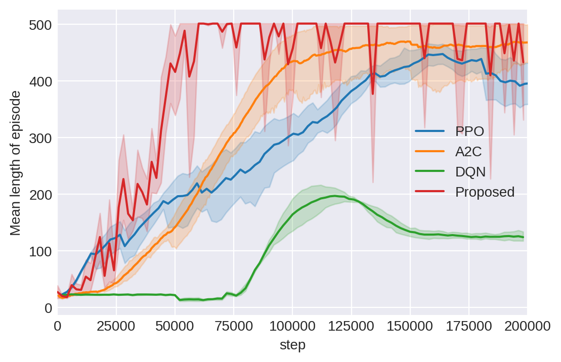
Figure 6: Performance of different baselines and our proposed algorithm on the CartPole-v1 benchmark.

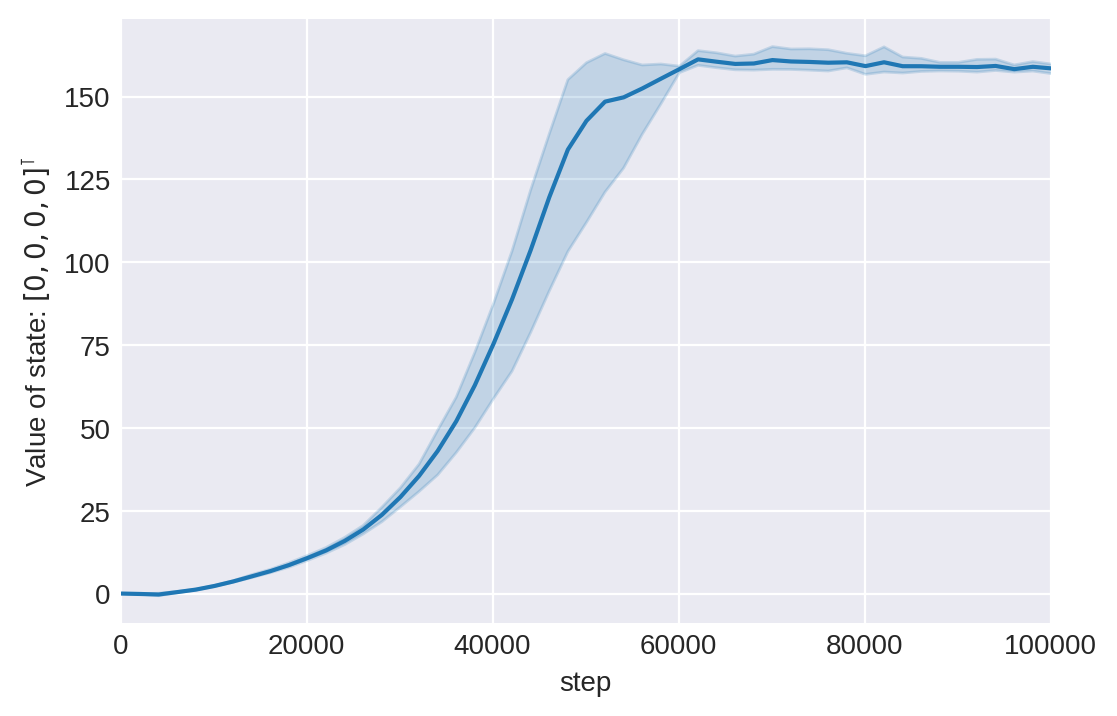
(a)

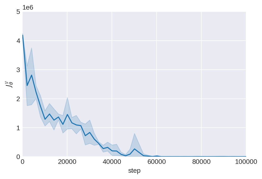
(b)

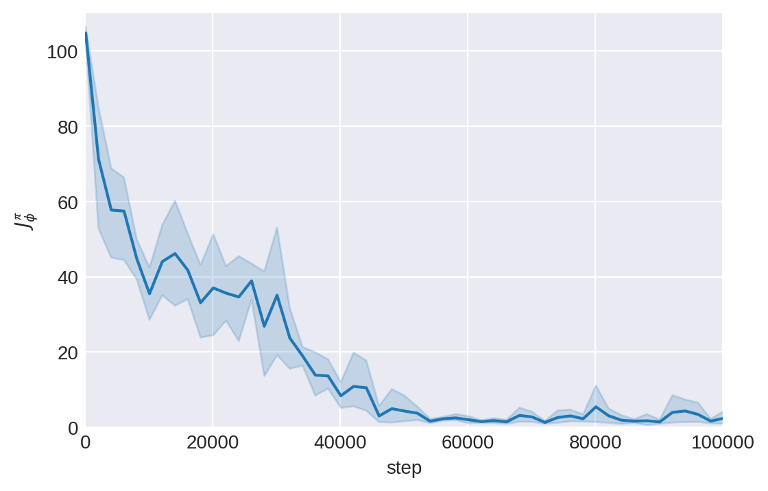
(c)

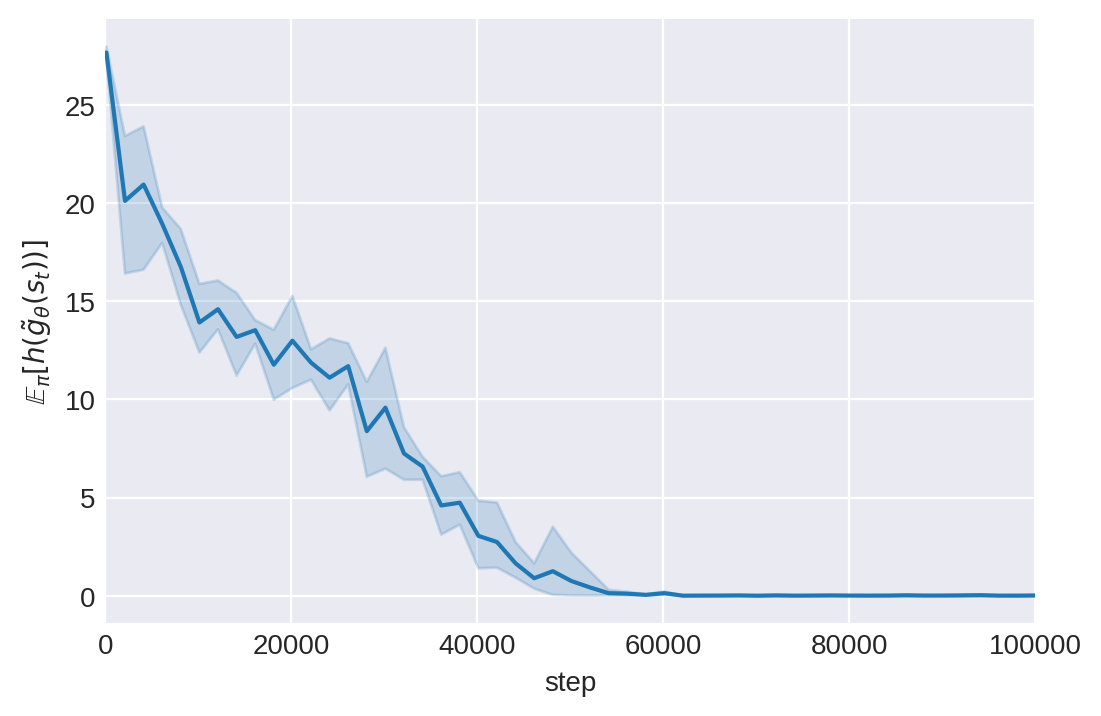
(d)

Figure 7: (a) Value of the initial state $\mathcal{V}(s_{0})$ versus training steps, where $s_{0}=[0,0,0,0]^{\intercal}$. (b) Loss of critic network $J^{\mathcal{V}}=\mathop{\bf E{}}\nolimits_{\rho\sim\mathcal{D}^{\pi}}[\mathcal{L}(\rho,\vec{\lambda},\vec{\nu})]$ versus training steps. (c) Loss of actor network $J^{\pi}=\mathop{\bf E{}}\nolimits_{\rho\sim\mathcal{D}^{\pi}}[\frac{1}{2}C(\rho)^{2}]$ versus training steps. (d) Evaluation of constraint $\mathop{\bf E{}}\nolimits_{\rho\sim\mathcal{D}^{\pi}}[h(\tilde{g}(s_{t}))]$ versus training steps.

To demonstrate the convergence of our proposed algorithm, we plot the value function of the initial state, loss of critic network, loss of actor network, and evaluation of the constraint $\mathop{\bf E{}}\nolimits_{\rho\sim\mathcal{D}^{\pi}}[h(\tilde{g}(s_{t}))]$ versus training steps in Fig. 7. Fig. 7(a) suggests our value function of the initial state converges after $6\times 10^{4}$ steps. Figure. 7(b) and Figure. 7(c) suggest $5\times 10^{4}$ steps is a critical training step point, where losses of actor and critic networks are close to zero. Near-zero losses of actor and critic networks match the step point where the length of episodes is close to the maximum length $500$ and the evaluation of the constraint decreases to zero shown in Fig. 6 and Fig. 7(d), respectively.

V-B Robot Motion Planning with a High-level Specification

We are interested in using the proposed algorithm to learn a policy in robot motion planning example with a high-level specification from Example 1, sequential visiting task. Recall that the goal is to maximize the probability that a car avoids obstacles and completes one of the following: (a) visit $A$ and do not visit $D$ or obstacles until $C$ is visited; (b) visit $D$ and do not visit $A$ or obstacles until $B$ is visited. The RC car travels within a workspace in Fig. 8, where $A,B,C$, and $D$ are regions of interest, and black rectangles are obstacles.

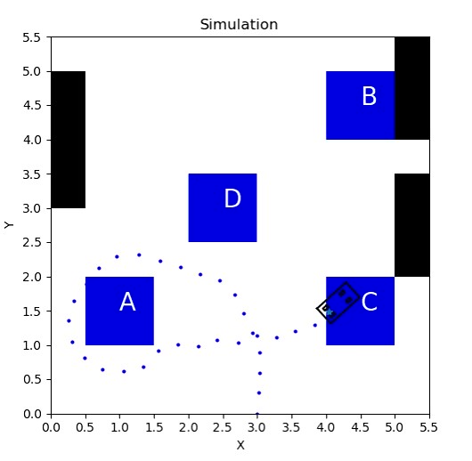
(a)

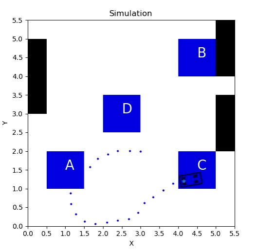
(b)

Figure 8: (a) A simulated trajectory staring from an initial state $[3,0,\pi/2]^{\intercal}$. (b) A simulated trajectory staring from a different initial state $[3,2,-\pi]^{\intercal}$ that is different from the initial state $[3,0,\pi/2]^{\intercal}$ during training.

We model the RC car as a Dubins car model. Let us briefly recall the dynamics of Dubins car defined as follows:

$$\dot{x} =v\cdot\cos\theta,$$

$$\dot{y} =v\cdot\sin\theta,$$

$$\dot{\theta} =u,$$

where $[x,y]$ denotes the car’s position, $\theta$ is the heading, the car is moving at a constant speed $v=0.3$ m/s, and the turn rate control $u\in\{-2\pi/15,0,2\pi/15\}$. The car starts at the initial state $[3,0,\pi/2]^{\intercal}$. For notational convenience, we use $\vec{z}=[x,y,\theta]^{\intercal}$ and $\vec{\dot{z}}=[\dot{x},\dot{y},\dot{\theta}]^{\intercal}$ to denote car’s state and velocity. Further, we let $\vec{z}_{t}$ and $\vec{\dot{z}}_{t}$ be the car’s state and velocity at time $t$, respectively. We capture the dynamic evolution of the car as follows:

$$\vec{z}_{t+\Delta t}=\vec{z}_{t}+\Delta\vec{z}_{noise}+\vec{\dot{z}}\cdot\Delta t,$$

where $\Delta t$ is the user-specified time unit, and $\Delta\vec{z}_{noise}$ is the noise. In our example, we have $\Delta t=1$ s and $\Delta\vec{z}_{noise}$ is the white noise with the standard deviation $10^{-2}$.

Typically, we give a reward of $1$ when the car completes the specification and $0$ otherwise. However, small rewards can be overshadowed when the entropy of policies is too large using the mellowmax operators. We amplify rewards as follows: A reward of $10$ is given when the car completes the specification; A reward of $-1$ is given whenever the car goes out of the workspace or hits the obstacles. Furthermore, to address the sparse reward issue, we define the reward signal as follows:

$$r(\vec{z},\vec{z}_{\mathsf{subgoal}})=\vec{\dot{z}}\cdot\frac{5\vec{d}}{\lvert\vec{d}\rvert},$$ (29)

where $\vec{z}$ is the current state, $\vec{z}_{\mathsf{subgoal}}$ is the current subgoal for the current automaton state, and $\vec{d}=[x_{\mathsf{subgoal}}-x,y_{\mathsf{subgoal}}-y]^{\intercal}$. We define the current subgoal for each automaton state as follows:

$$\vec{z}_{\mathsf{subgoal}}=\begin{cases}[1.25,1.25]^{\intercal},\text{ if }q=q_{0},\\ [4.25,4.25]^{\intercal},\text{ if }q=q_{1},\\ [4.25,1.25]^{\intercal},\text{ if }q=q_{2}.\end{cases}$$ (30)

Note that we do not define the subgoal for $q_{3}$ since the car has satisfied the specification. To demonstrate our trained policy can handle different initial states, we sample two trajectories from two initial states: (a) $[3,0,\pi/2]^{\intercal}$ is the same as the one during training and (b) $[3,2,-\pi]^{\intercal}$ is different from the one during training, and plot them in Fig. 8.

TABLE III: Success Rates of Sequential Visiting Task

Description	Success Rate
Single neural network	$26\%$
Modular learning	$49\%$
Modular learning $+$ topological order	$71.5\%$

We propose topological order to address the reward sparsity and modular learning to break down the ordinal relation between automaton states. To demonstrate the efficacy of both techniques, we compare our proposed method with a single neural network, modular learning, and modular learning with topological order. We plot corresponding values of the initial state in Fig. 9 and list the success rates of the sequential visiting task (over 200 simulations) in Table III. In the case of a single neural network for the entire product MDP, the input of the neural network is a $4$-dimension vector, where the first $3$ elements are the car’s state, and the last element is the automaton state. For modular learning, the input of the neural network is only the car’s state.

As listed in Tab III, implementing modular learning increases the success rate dramatically, indicating the ordinal relationship is disrupted and provides better approximations for value and policy function. Given the same training steps, the success rate with the topological order is much higher than the one without the topological order. The above observation from Tab III matches the result in Fig. 9, where the value of modular learning with topological order has the highest value and fastest convergence. Theoretically, the one with the topological order shall at least perform as well as the one without the topological order. Such improvement in the performance demonstrates that the topological order can guide value backups and accelerate the learning process.

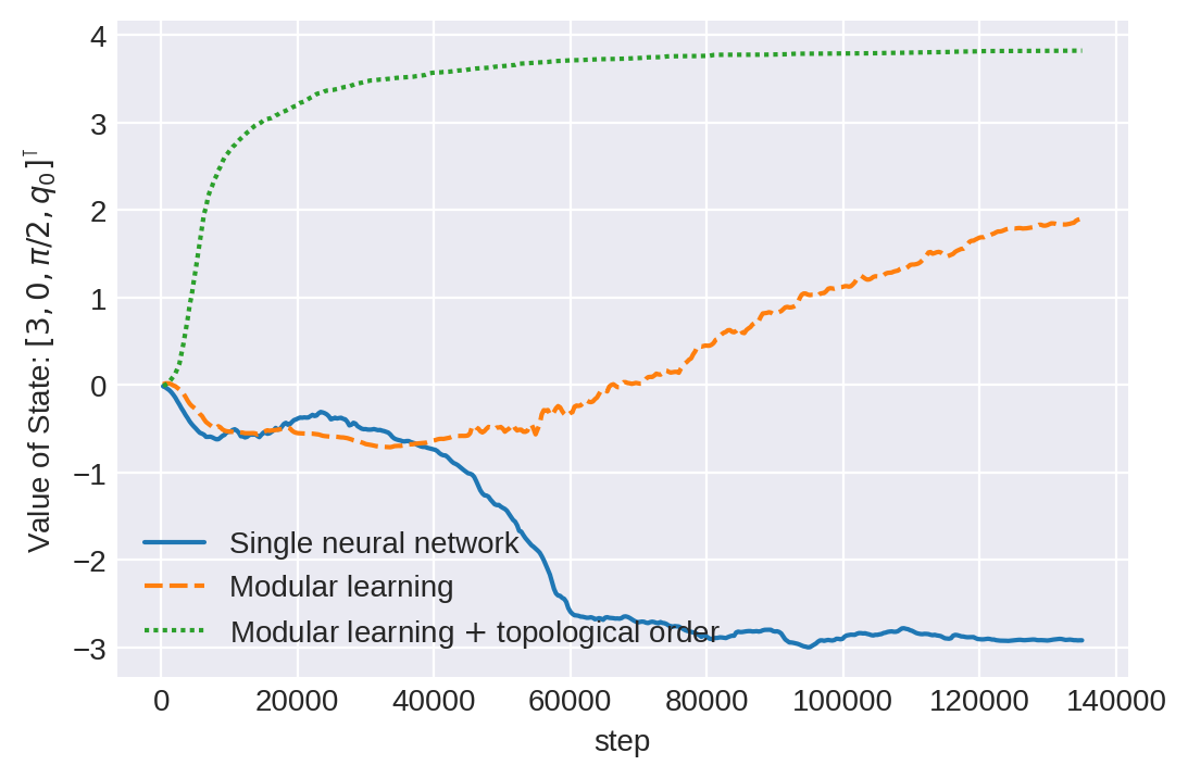
Figure 9: Values of initial state $\mathcal{V}(z_{0})$ versus training steps, where $z_{0}=[3,0,\pi/2,q_{0}]^{\intercal}$.

We provide a video to demonstrate the success of learning a controller that satisfies the specification. The car uses AprilTags in the Tag36h11 set as fiducial markers for localization [29].

We run our algorithms on an Ubuntu 20.04 machine with AMD Ryzen 9 5900X CPU, 32 GB RAM, and NVIDIA GeForce RTX 3060. The computational time of computing a policy in CartPole is about $4$ hours, and the computational times of computing a policy in Dubins car environment are about $17$ min, $23$ min, and $53$ min for single neural network, modular learning, and modular learning with topological order, respectively. We find that the long computational time for CartPole is because of trajectory simulations for computing the mean length of episode . The reason for the computational time of modular learning with topological order is $2$ times these of modular learning and single neural network is because, in our example, we have the set of level sets $\{\operatorname{\mathcal{L}}_{0},\operatorname{\mathcal{L}}_{1},\operatorname{\mathcal{L}}_{2}\}$, where the value of any state $(s,q)\in S\times\operatorname{\mathcal{L}}_{0}$ equals to $0$. So we need to learn values for $\operatorname{\mathcal{L}}_{1}$ and $\operatorname{\mathcal{L}}_{2}$.

VI Related Work

Formal policy synthesis for stochastic systems has received substantial research attention. Researchers are especially interested in the problem of synthesizing a policy that maximizes the satisfaction probability of given high-level specifications expressed in LTL. This satisfaction problem is first introduced by [30]. Approaches to solving this satisfaction problem often fall into two categories: (a) automaton-based approach and (b) non-automaton-based approach.

Non-automaton-based approaches [31, 32, 33, 34] formulate a constrained optimization, where LTL formulas are encoded in constraints. Such constrained optimization approaches leverage the empirical performance of state-of-art solvers and enjoy great successes in theoretical results [32] as well as the application [35] within the control community. Specifically, authors [32] propose a mixed-integer linear programming (MILP) for optimal control of nonlinear systems. They encode LTL specifications as mixed-integer linear constraints to avoid the construction of the task automaton. Still, mixed-integer linear programming suffers from mathematical difficulties when the problem size becomes large due to solving an MILP is an NP-complete problem. Authors of [34] investigate a multi-robot motion planning problem with tasks expressed in a subset of LTL formulas. They first formulate the feasibility problem over a combination of boolean and convex constraints. They then adopt a satisfiability modulo convex programming approach to decompose the problem into efficiently solvable smaller problems. These works require system models because of the need for explicit constraints on system dynamics.

Alternatively, the automaton-based approach [30, 36, 37, 38, 39] takes the explicitly/on-the-fly product between the dynamic system and the corresponding task automaton. Then they solve the optimal planning problem over this product system in a broad range of methodologies, including optimization and RL.

Authors [30] take the optimization route. They first translate the LTL formulas into deterministic Rabin automaton (DRA), where a LTL formula is translated into a DRA. After the LTL-DRA conversion, they use an MDP to model the stochastic system. Given such a DRA and MDP, they build a product MDP and formulate it as a linear programming problem. However, this work requires the knowledge of the model, i.e., the transition probabilities, and the considered state space is discrete.

RL has proven to be a powerful class of algorithms for learning a control policy in a variety of applications from robotics [40], flight control [41], resource management [42], and gaming [43]. Learning in an interactive environment in RL falls into two categories: (a) model-based methods (e.g., value iteration and policy iteration) and (b) model-free methods (e.g., Q-learning, DQN, deep deterministic policy gradient (DDPG)). Existing works for formal policy synthesis [36, 37, 38, 39] adopt learning an approximate model or model-free methods to address the necessities of system model knowledge. For a model-based method [36], authors first propose an algorithm that learns a probably approximately correct MDP. Then they apply value iteration (model-based) to synthesize a policy. On the other side, authors [37] propose a model-free RL algorithm, i.e., Q-learning, to produce a policy for an on-the-fly product MDP with a synchronous reward function based on the acceptance condition. The above works investigate the policy synthesis in the discrete state space, while continuous state spaces are more often encountered in the real world. Later, authors [38] extend their work into the continuous state space, which leads to the first model-free RL policy synthesis algorithm in continuous-sate MDP, although they leverage some existing RL algorithms. Another way to handle the continuous state space is hierarchical planning [44, 45, 46]. Authors [45] develop a compositional learning approach, called DIRL, that interleaves model-based high-level planning and model-free RL. First, DIRL encodes the specification as an abstract graph; intuitively, vertices and edges of the graph correspond to regions of the state space and simpler sub-tasks, respectively. Their approach then incorporates RL to learn neural network policies for each edge (sub-task) within a Dijkstra-style planning algorithm to compute a high-level plan in the graph. However, high-level planning still requires a model of the dynamic system.

VII Conclusion

This paper proposes a comprehensive formal policy synthesis framework for continuous-state stochastic dynamic systems with high-level specifications. We introduce the topological order to overcome the reward sparsity and prove that the topological order does not affect the optimality of the value function. To overcome the continuous/hybrid state space, we present a sequential, actor-critic RL algorithm, where topological order still applies. We provide proof of optimality and convergence of this RL algorithm in a tabular case. We further use modular learning to prevent the approximate value/policy function from being ranked by assigning integer numbers to automaton states. Our proposed algorithm matches or beats baselines in CartPole. We demonstrate the efficacy of our policy synthesis framework on a Dubins car with a high-level specification, where a video validates the success of learning a controller that satisfies the specification. The results suggest that the topological order can relieve the sparse reward issue, and modular learning can break the ordinal relationship between the automaton states.

Lening Li (Student Member, IEEE) received a B.S. degree in Information Security (Computer Science) from Harbin Institute of Technology, China in 2014, and an M.S. degree in Computer Science from Worcester Polytechnic Institute, Worcester, MA, USA, in 2016. He is currently pursuing a Ph.D. degree in Robotics Engineering at Worcester Polytechnic Institute, Worcester, MA, USA. His research interests include reinforcement learning, stochastic control, game theory, and formal methods.

Zhentian Qian (Student Member, IEEE) received a B.Eng. degree in Electronic Information Engineering from Zhejiang University, China in 2016, and an M.S. degree in Electrical Engineering from Zhejiang University, China in 2019. He is currently pursuing a Ph.D. degree in Robotics Engineering at Worcester Polytechnic Institute, Worcester, MA, USA. His research interests include computer vision, simultaneous localization and mapping, probabilistic decision-making, and formal methods.

References

- [1] X. Li, C.-I. Vasile, and C. Belta, “Reinforcement learning with temporal logic rewards,” in 2017 IEEE/RSJ International Conference on Intelligent Robots and Systems (IROS). IEEE, 2017, pp. 3834–3839.
- [2] N. Bernini, M. Bessa, R. Delmas, A. Gold, E. Goubault, R. Pennec, S. Putot, and F. Sillion, “Reinforcement learning with formal performance metrics for quadcopter attitude control under non-nominal contexts,” arXiv preprint arXiv:2107.12942, 2021.
- [3] A. K. Bozkurt, Y. Wang, and M. Pajic, “Secure planning against stealthy attacks via model-free reinforcement learning,” in 2021 IEEE International Conference on Robotics and Automation (ICRA). IEEE, 2021, pp. 10 656–10 662.
- [4] C. A. Belta, R. Majumdar, M. Zamani, and M. Rungger, “Formal Synthesis of Cyber-Physical Systems (Dagstuhl Seminar 17201),” Dagstuhl Reports, vol. 7, no. 5, pp. 84–96, 2017. [Online]. Available: http://drops.dagstuhl.de/opus/volltexte/2017/8281
- [5] Z. Manna and A. Pnueli, The temporal logic of reactive and concurrent systems: Specification. Springer Science & Business Media, 2012.
- [6] A. Duret-Lutz, A. Lewkowicz, A. Fauchille, T. Michaud, E. Renault, and L. Xu, “Spot 2.0—a framework for ltl and -automata manipulation,” in International Symposium on Automated Technology for Verification and Analysis. Springer, 2016, pp. 122–129.
- [7] L. Z. Yuan, M. Hasanbeig, A. Abate, and D. Kroening, “Modular deep reinforcement learning with temporal logic specifications,” arXiv preprint arXiv:1909.11591, 2019.
- [8] G. Tesauro et al., “Temporal difference learning and td-gammon,” Communications of the ACM, vol. 38, no. 3, pp. 58–68, 1995.
- [9] D. P. De Farias and B. Van Roy, “The linear programming approach to approximate dynamic programming,” Operations research, vol. 51, no. 6, pp. 850–865, 2003.
- [10] A. Pnueli and R. Rosner, “On the synthesis of a reactive module,” in Proceedings of the 16th ACM SIGPLAN-SIGACT symposium on Principles of programming languages, 1989, pp. 179–190.
- [11] O. Kupferman and M. Y. Vardi, “Model checking of safety properties,” Formal Methods in System Design, vol. 19, no. 3, pp. 291–314, 2001.
- [12] C. Baier and J.-P. Katoen, Principles of model checking. MIT press, 2008.
- [13] H. Mao, Y. Chen, M. Jaeger, T. D. Nielsen, K. G. Larsen, and B. Nielsen, “Learning markov decision processes for model checking,” arXiv preprint arXiv:1212.3873, 2012.
- [14] D. P. Bertsekas et al., “Dynamic programming and optimal control 3rd edition, volume ii,” Belmont, MA: Athena Scientific, 2011.
- [15] P. Dai, D. S. Weld, J. Goldsmith et al., “Topological value iteration algorithms,” Journal of Artificial Intelligence Research, vol. 42, pp. 181–209, 2011.
- [16] G. Froyland, “Statistically optimal almost-invariant sets,” Physica D: Nonlinear Phenomena, vol. 200, no. 3-4, pp. 205–219, 2005.
- [17] V. Aho Alfred, E. Hopcroft John, D. Ullman Jeffrey, V. Aho Alfred, H. Bracht Glenn, D. Hopkin Kenneth, C. Stanley Julian, B. Jean-Pierre, B. A. Samler, B. A. Peter et al., Data structures and algorithms. USA: Addison-Wesley, 1983.
- [18] T. Haarnoja, A. Zhou, P. Abbeel, and S. Levine, “Soft actor-critic: Off-policy maximum entropy deep reinforcement learning with a stochastic actor,” in International conference on machine learning. PMLR, 2018, pp. 1861–1870.
- [19] R. S. Sutton and A. G. Barto, Reinforcement learning: An introduction. MIT press, 2018.
- [20] O. Nachum, M. Norouzi, K. Xu, and D. Schuurmans, “Bridging the gap between value and policy based reinforcement learning,” arXiv preprint arXiv:1702.08892, 2017.
- [21] T. Degris, M. White, and R. S. Sutton, “Off-policy actor-critic,” arXiv preprint arXiv:1205.4839, 2012.
- [22] J. Schulman, F. Wolski, P. Dhariwal, A. Radford, and O. Klimov, “Proximal policy optimization algorithms,” arXiv preprint arXiv:1707.06347, 2017.
- [23] V. Mnih, K. Kavukcuoglu, D. Silver, A. Graves, I. Antonoglou, D. Wierstra, and M. Riedmiller, “Playing atari with deep reinforcement learning,” arXiv preprint arXiv:1312.5602, 2013.
- [24] V. Mnih, A. P. Badia, M. Mirza, A. Graves, T. Lillicrap, T. Harley, D. Silver, and K. Kavukcuoglu, “Asynchronous methods for deep reinforcement learning,” in International conference on machine learning. PMLR, 2016, pp. 1928–1937.
- [25] J. ASHTON, M. E. Spencer, and S. Hunter, “Autonomous rc car platform,” Ph.D. dissertation, Worcester Polytechnic Institute, 2019.
- [26] “Slash 4x4 platinum: 1/10 scale 4wd electric short course truck with low cg chassis,” (Accessed on 02/27/2022). [Online]. Available: https://traxxas.com/products/models/electric/6804Rslash4x4platinum
- [27] G. Brockman, V. Cheung, L. Pettersson, J. Schneider, J. Schulman, J. Tang, and W. Zaremba, “Openai gym,” arXiv preprint arXiv:1606.01540, 2016.
- [28] A. G. Barto, R. S. Sutton, and C. W. Anderson, “Neuronlike adaptive elements that can solve difficult learning control problems,” IEEE transactions on systems, man, and cybernetics, no. 5, pp. 834–846, 1983.
- [29] E. Olson, “Apriltag: A robust and flexible visual fiducial system,” in 2011 IEEE international conference on robotics and automation. IEEE, 2011, pp. 3400–3407.
- [30] X. C. D. Ding, S. L. Smith, C. Belta, and D. Rus, “Ltl control in uncertain environments with probabilistic satisfaction guarantees,” IFAC Proceedings Volumes, vol. 44, no. 1, pp. 3515–3520, 2011.
- [31] S. Karaman, R. G. Sanfelice, and E. Frazzoli, “Optimal control of mixed logical dynamical systems with linear temporal logic specifications,” in 2008 47th IEEE Conference on Decision and Control. IEEE, 2008, pp. 2117–2122.
- [32] E. M. Wolff, U. Topcu, and R. M. Murray, “Optimization-based trajectory generation with linear temporal logic specifications,” in 2014 IEEE International Conference on Robotics and Automation (ICRA). IEEE, 2014, pp. 5319–5325.
- [33] Y. Kwon and G. Agha, “Ltlc: Linear temporal logic for control,” in International Workshop on Hybrid Systems: Computation and Control. Springer, 2008, pp. 316–329.
- [34] Y. Shoukry, P. Nuzzo, A. Balkan, I. Saha, A. L. Sangiovanni-Vincentelli, S. A. Seshia, G. J. Pappas, and P. Tabuada, “Linear temporal logic motion planning for teams of underactuated robots using satisfiability modulo convex programming,” in 2017 IEEE 56th annual conference on decision and control (CDC). IEEE, 2017, pp. 1132–1137.
- [35] S. Karaman and E. Frazzoli, “Linear temporal logic vehicle routing with applications to multi-uav mission planning,” International Journal of Robust and Nonlinear Control, vol. 21, no. 12, pp. 1372–1395, 2011.
- [36] J. Fu and U. Topcu, “Probably approximately correct mdp learning and control with temporal logic constraints,” arXiv preprint arXiv:1404.7073, 2014.
- [37] M. Hasanbeig, Y. Kantaros, A. Abate, D. Kroening, G. J. Pappas, and I. Lee, “Reinforcement learning for temporal logic control synthesis with probabilistic satisfaction guarantees,” in 2019 IEEE 58th Conference on Decision and Control (CDC). IEEE, 2019, pp. 5338–5343.
- [38] M. Hasanbeig, A. Abate, and D. Kroening, “Certified reinforcement learning with logic guidance,” arXiv preprint arXiv:1902.00778, 2019.
- [39] A. Lavaei, F. Somenzi, S. Soudjani, A. Trivedi, and M. Zamani, “Formal controller synthesis for continuous-space mdps via model-free reinforcement learning,” in 2020 ACM/IEEE 11th International Conference on Cyber-Physical Systems (ICCPS). IEEE, 2020, pp. 98–107.
- [40] J. Kober, J. A. Bagnell, and J. Peters, “Reinforcement learning in robotics: A survey,” The International Journal of Robotics Research, vol. 32, no. 11, pp. 1238–1274, 2013.
- [41] P. Abbeel, A. Coates, M. Quigley, and A. Y. Ng, “An application of reinforcement learning to aerobatic helicopter flight,” Advances in neural information processing systems, vol. 19, p. 1, 2007.
- [42] H. Mao, M. Alizadeh, I. Menache, and S. Kandula, “Resource management with deep reinforcement learning,” in Proceedings of the 15th ACM workshop on hot topics in networks, 2016, pp. 50–56.
- [43] V. Mnih, K. Kavukcuoglu, D. Silver, A. A. Rusu, J. Veness, M. G. Bellemare, A. Graves, M. Riedmiller, A. K. Fidjeland, G. Ostrovski et al., “Human-level control through deep reinforcement learning,” nature, vol. 518, no. 7540, pp. 529–533, 2015.
- [44] X. Ding, S. L. Smith, C. Belta, and D. Rus, “Optimal control of markov decision processes with linear temporal logic constraints,” IEEE Transactions on Automatic Control, vol. 59, no. 5, pp. 1244–1257, 2014.
- [45] K. Jothimurugan, S. Bansal, O. Bastani, and R. Alur, “Compositional reinforcement learning from logical specifications,” Advances in Neural Information Processing Systems, vol. 34, 2021.
- [46] P. Schillinger, M. Bürger, and D. V. Dimarogonas, “Hierarchical ltl-task mdps for multi-agent coordination through auctioning and learning,” The international journal of robotics research, 2019.