Visual DNA:
Representing and Comparing Images using Distributions of Neuron Activations

Abstract

Selecting appropriate datasets is critical in modern computer vision. However, no general-purpose tools exist to evaluate the extent to which two datasets differ. For this, we propose representing images – and by extension datasets – using Distributions of Neuron Activations (DNAs). DNAs fit distributions, such as histograms or Gaussians, to activations of neurons in a pre-trained feature extractor through which we pass the image(s) to represent. This extractor is frozen for all datasets, and we rely on its generally expressive power in feature space. By comparing two DNAs, we can evaluate the extent to which two datasets differ with granular control over the comparison attributes of interest, providing the ability to customise the way distances are measured to suit the requirements of the task at hand. Furthermore, DNAs are compact, representing datasets of any size with less than 15 megabytes. We demonstrate the value of DNAs by evaluating their applicability on several tasks, including conditional dataset comparison, synthetic image evaluation, and transfer learning, and across diverse datasets, ranging from synthetic cat images to celebrity faces and urban driving scenes.

1 Introduction

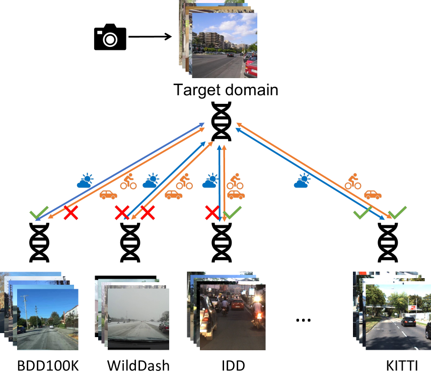
(a) When deploying a vision model in a new target domain, selecting models pre-trained on the most relevant datasets can help. However, there are no methods to measure dataset similarities automatically. A general distance between datasets would be sensitive to many variation types, but DNAs provide sufficient granularity to customise the comparison to focus on features of interest. For example, DNA comparisons can be customised to ignore weather conditions or focus on semantic content.

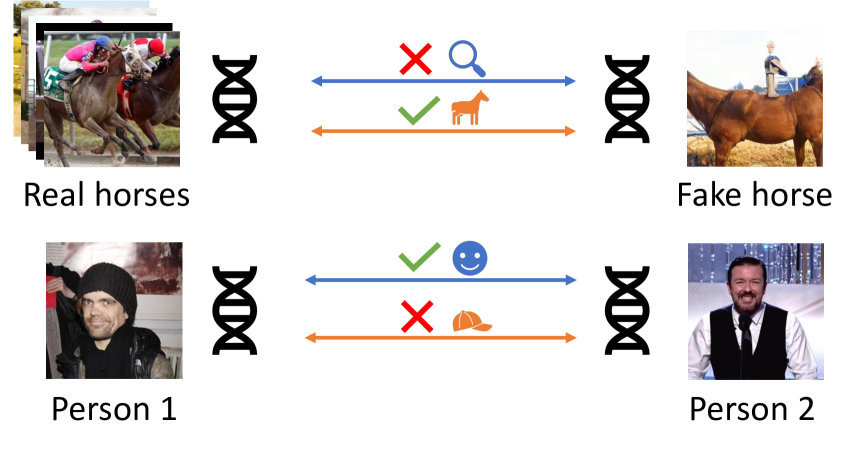
(b) The DNA can also be used to compare individual images to datasets – for example, to measure the realism and semantic consistency of a synthetic image – or pairs of images – for example, to verify the presence of similar attributes such as smiling or wearing a hat.

Figure 1: Example use-cases of the DNA representation.

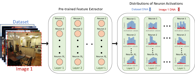
Figure 2: We propose representing images by passing them through a pre-trained frozen feature extractor network and collecting neuron activations. We then create a descriptor called the DNA by fitting a distribution (the histogram in the illustration) to the activations at each neuron. We can quantitatively measure the similarity of different datasets or images by comparing their DNAs. Neuron combination strategies that are sensitive to specific attributes can also allow for customised comparisons of DNAs.

Being able to compare datasets and understanding how they differ is critical for many applications, including deciding which labelled dataset is best to train a model for deployment in an unlabelled application domain, sequencing curricula with gradually increasing domain gap, evaluating the quality of synthesised images, and curating images to mitigate dataset biases.

However, we currently lack such capabilities. For example, driving datasets available covering many domains [62, 9, 16, 17, 4, 54, 35, 64, 22, 2] were collected under diverse conditions typically affecting image appearance (e.g. location, sensor configuration, weather conditions, and post-processing). Yet, users are limited to coarse or insufficient meta-information to understand these differences. Moreover, depending on the application, it might be desirable to compare datasets only on controlled sets of attributes while ignoring others. For self-driving, these may be weather, road layout, driving patterns, or other agents’ positions.

We propose representing datasets using their Distributions of Neuron Activations (DNAs), allowing efficient and controllable dataset and image comparisons (Fig. 1). The DNA creation exploits the recent progress in self-supervised representation learning [18, 13] and extracts image descriptors directly from patterns of neuron activations in neural networks (NNs). As illustrated in Fig. 2, DNAs are created by passing images through an off-the-shelf pre-trained frozen feature extraction model and fitting a distribution (e.g. histogram or Gaussian) to the activations observed at each neuron. This DNA representation contains multi-granular feature information and can be compared while controlling attributes of interest, including low-level and high-level information. Our technique was designed to make comparisons easy, avoiding high-dimensional feature spaces, data-specific tuning of processing algorithms, model training, or any labelling. Moreover, saving DNAs requires less than 15 megabytes, allowing users to easily inspect the DNA of large corpora and compare it to their data before committing resources to a dataset. We demonstrate the results of using DNAs on real and synthetic data in multiple tasks, including comparing images to images, images to datasets, and datasets to datasets. We also demonstrate its value in attribute-based comparisons, synthetic image quality assessment, and cross-dataset generalisation prediction.

2 Related Works

2.1 Studying Image Datasets

Early dataset studies focused on the limitations of the datasets available at the time. Ponce et al. [43] highlighted the need for more data, realism, and diversity, focusing on object recognition and qualitative analysis (e.g. “average” images for each class). Torralba and Efros [56] found evidence of significant biases in datasets by assessing the ability of a classifier to recognise images from different datasets and measuring cross-dataset generalisation of object classification and detection models. Nowadays, datasets abound, and the approaches used to compare them in those early works would be prohibitive to scale or generalise, often requiring training models for each dataset of interest and access to labels.

Compressed datasets representations allow learning models with comparable properties with reduced dataset sizes. Dataset distillation approaches [59] synthesise a small sample set to approximate the original data when used to train a model. Core-set selection approaches [15], instead, select existing samples, with image-based applications including visual-experience summarisation [42] and active learning [50]. While achieving compression of important data properties, these approaches do not produce representations that allow easy dataset comparisons, as our DNA does. Modelverse [34] performs a content-based search of generative models. Similarly to DNAs, they represent multiple datasets – generated by different generative models – using distribution statistics of extracted features from the images. However, their work does not focus on granular and controllable comparisons but on matching a query to the closest distribution.

Synthetic data evaluation for generative models such as Generative Adversarial Networks (GANs) [3] is usually framed as a dataset comparison problem, measuring a distance between datasets of real and fake images. One of the most widely used metrics is the Fréchet Inception Distance (FID) [21], which embeds all images into the feature space of a specific layer of the Inception-v3 network [55]. A multivariate Gaussian is fit to each real and fake embedding, and the Fréchet distance (FD) between these distributions is computed. The Kernel Inception Distance (KID) [1] is another popular approach, which computes the squared maximum mean discrepancy between Inception-v3 embeddings. There are many other variations, such as using precision and recall metrics for distributions [10, 30, 49, 51], density and coverage [37], or rarity score [19]. These approaches rely on high-dimensional features from one layer, while our approach considers neuron activations across layers. Furthermore, while these measure dataset differences, they have mainly been employed to compare real and synthetic datasets within the same domain, not real ones with significant domain shifts. Moreover, recent evidence suggests the embeddings typically used can cause a heavy bias towards ImageNet class probabilities [29], motivating more perceptually-uniform distribution metrics. Additionally, these high-dimensional embeddings make gathering information about specific attributes of interest challenging and lead to computational issues (e.g. when clustering).

2.2 Representation Learning

Feature extractors can provide useful multi-granular features (e.g. containing information about low-level lighting conditions but also the high-level semantics), motivating our design of DNAs. Work on the interpretability of NNs supports this assumption. Indeed, Olah et al. [39, 5] explored the idea that NNs learn features as fundamental units and that analogous features form across different models and tasks. Neurons can react more to specific inputs, such as edges or objects [40]. Combining neuron activations from several images can be a good way to investigate what a network has learned through an activation atlas [8].

Existing uses of pre-trained feature extractors include evaluating computer vision tasks such as Inception-v3 features for FID and KID, as above. Pre-trained networks on large datasets also provide generally useful representations [24], which are often fine-tuned for specific applications. Notably, Evci et al. [14] found that selecting features from subsets of neurons from all layers of a pre-trained network allows better fine-tuning of a classifier head for transfer learning than using only the last layer, suggesting that relevant features are accessible by selecting appropriate neurons. Moreover, a pre-trained VGG network [52] has been used to improve the perceptual quality of synthetic images [46, 60] or to judge photorealism [65, 46].

Self-supervised training relies on pretext tasks, foregoing labelled data and learning over larger corpora, yielding better representations [24]. Morozov et al. [36] showed that using embeddings from self-supervised networks such as a ResNet50 [20] trained with SwAV [6] leads to FID scores better aligned to human quality judgements when evaluating generative models. We explore different feature extractors but exploit a ViT-B/16 [11] trained with Mugs [67] by default, a recent multi-granular feature technique.

2.3 The need for a more general tool

FID [21] or KID [1] use representation learning to tackle similar tasks to ours; yet, our formulation extends their applicability. Quantitative and holistic comparisons between different real datasets have been overlooked, despite being critical to tasks such as transfer or curriculum learning. We argue that a general data-comparison tool must allow selecting attributes of interest after having extracted a reasonably compact representation of the image(s) and permit the user to customise the distance between representations.

3 DNA - Distributions of Neuron Activations

Our system is designed around the principle of decomposing images into simple conceptual building blocks that, in combination, constitute uniqueness. Yet, to cover all possible axes of variations, it is infeasible to specify those building blocks manually. While we cannot usually link each neuron of a NN to a human concept [40], we show that they provide a useful granular decomposition of images.

Keeping track of neuron activations independently allows us to combine their statistics and study conceptually-meaningful attributes of interest. As the activations at each neuron are scalar, they can easily be gathered in 1D histograms or univariate Gaussians. While we would ideally track dependencies between neurons, this is too costly to include in our representation. Nevertheless, we show experimentally that many applications still benefit from DNAs.

3.1 Distribution choice

As in Fig. 2, in this section, we formulate DNAs using histograms to fit each neuron’s activations distribution. Histograms are a good choice because they do not make assumptions about the underlying distribution; however, we can also consider other distribution approximations. We also experiment with univariate Gaussians to approximate the activations of each neuron and produce a DNA, allowing us to describe distributions with only two parameters. We denote versions using histograms and Gaussians as DNA${}^{\text{hist.}}$ and DNA${}^{\text{Gauss.}}$, respectively.

3.2 Generating the DNA from images

We consider a dataset of images $\mathcal{I}$ where $|\mathcal{I}|~{}\geq~{}1$. We also have a pre-trained feature extractor $\mathcal{F}$ with $L$ layers $\mathcal{L}$ manually defined as being of interest, and a set $\mathcal{N}$ of all neurons in those layers. Each layer $l\in\mathcal{L}$ is composed of $N_{l}$ neurons, each producing a feature map of spatial dimensions $S_{h}^{l}\times S_{w}^{l}$. We can perform a forward pass $\mathcal{F}(i)$ of an image $i\in\mathcal{I}$ and observe the feature map $f^{l}_{i}$ obtained at each layer $l$ which has dimensions $N_{l}~{}\times~{}S_{h}^{l}~{}\times~{}S_{w}^{l}$. For each neuron $n\in\mathcal{N}$ fed with image $i$, we define a histogram $h_{i}^{n}\in\mathbb{N}^{B}$ with $B$ pre-defined uniform bins where bin edges are denoted $b_{0},b_{1},\ldots,b_{B}$. The count $h^{n}_{i}[k]$ in the bin of index $k$ for neuron $n$ of layer $l$ is found by accumulating over all spatial dimensions that fall within the bin’s edges:

$$h^{n}_{i}[k]=\sum^{S_{h}^{l}}_{s_{h}}\sum^{S_{w}^{l}}_{s_{w}}\begin{cases}1,&\text{if }f_{i}^{l}[n,s_{h},s_{w}]\in\left[b_{k},b_{k+1}\right)\\ 0,&\text{otherwise}\\ \end{cases}$$ (1)

The resulting image’s DNA${}^{\text{hist.}}$ can then be accumulated to represent the dataset $\mathcal{I}$ as $H=\{\mathcal{H}^{n}\}$ for each neuron $n\in\mathcal{N}$, where the element $k$ of $\mathcal{H}^{n}$ can be calculated as:

$$\mathcal{H}^{n}[k]=\sum_{i\in\mathcal{I}}h^{n}_{i}[k]$$ (2)

3.3 Comparing DNAs

Now, comparing DNAs${}^{\text{hist.}}$ reduces to comparing 1D histograms for neurons of interest. Depending on the use case, different distances can be considered. Some tasks might need a distance to be asymmetrical and keep track of original histogram counts, while normalised counts and symmetric distances might be more appropriate for others.

To demonstrate straightforward uses of the representation, we experiment with a widely accepted histogram comparison metric: the Earth Mover’s Distance (EMD). Earlier works have argued that the EMD is a good metric for image retrieval using histograms [48], with examples of retrieval based on colour and texture. This work uses its normalised version, equivalent to the Mallows or first Wasserstein distance [32]. The EMD can be interpreted as the minimum cost of turning one distribution into another, combining the amount of distribution mass to move and the distance. Specifically, given the normalised, cumulative histogram

$$\mathcal{F}^{n}[k]=\sum^{k}_{j=0}\frac{\mathcal{H}^{n}[j]}{\left\lVert\mathcal{H}^{n}\right\lVert_{1}}\text{ where }k\in 0,\ldots,B-1$$ (3)

we can easily compute the EMD between two histograms:

$$\text{EMD}(\mathcal{H}^{n}_{1},\mathcal{H}^{n}_{2})=\sum^{B-1}_{k=0}\lvert{\mathcal{F}}^{n}_{1}[k]-\mathcal{F}^{n}_{2}[k]\rvert$$ (4)

As every neuron $n$ is independent in the EMD formulation, we can vary the contribution of each to the calculation of the total distance. This allows us to treat neurons differently, e.g. when wanting to customise the distance to ignore specific attributes, as presented in Sec. 5.3. For this, we introduce the use of a simple linear combination of the histograms through scalar weights $W^{n}$ for each neuron $n$:

$$\text{EMD}_{W}(H_{1},H_{2})=\sum_{n\in\mathcal{N}}W^{n}{\text{EMD}(\mathcal{H}^{n}_{1},\mathcal{H}^{n}_{2})}$$ (5)

In the special case of $W^{n}={1}/|\mathcal{N}|$, we obtain $\text{EMD}_{\text{avg}}$ as the average EMD over individual neuron comparisons.

4 Experimental settings

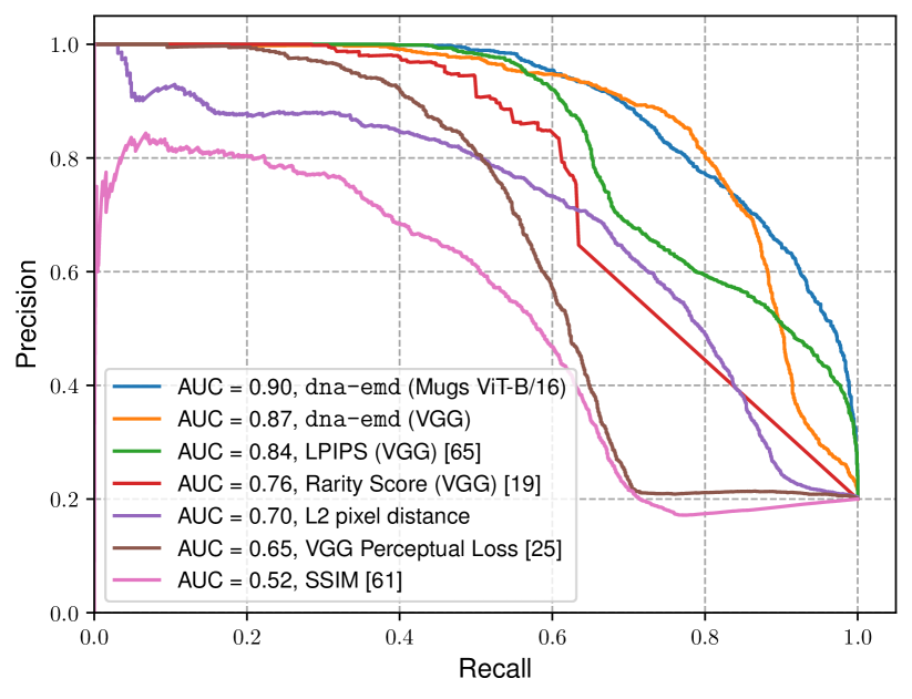
Figure 3: Precision-Recall curves and Area Under the Curve (AUC) for retrieving 2000 individual augmented Cityscapes images mixed with 8000 images from four other datasets. The retrieval compares these images to a reference set of 500 distinct non-augmented Cityscapes images.

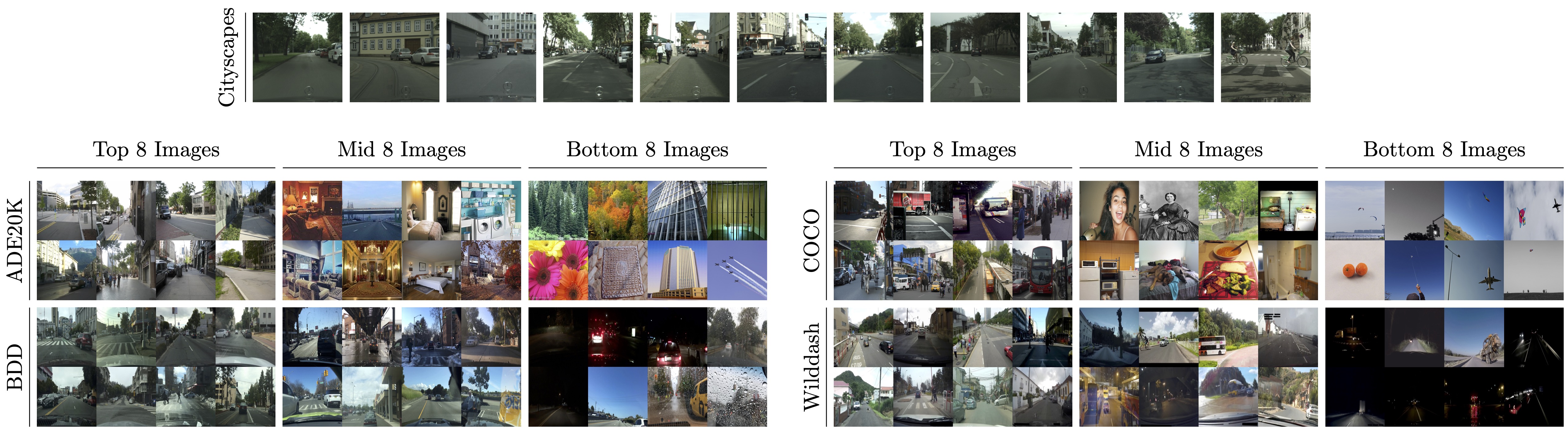
Figure 4: Images from different datasets organised by dna-emd over all neurons against Cityscapes. We successfully discriminate based on the scene type and its visual aspect. COCO and ADE20K images get poorly ranked when they do not contain city street scenes. The visual aspect and image quality are also considered, as seen with poorly ranked images when Wilddash images have different lighting or BDD images have challenging conditions such as rain on the windshield. Images ranked in the middle for BDD tend to contain scenes without any obvious anomaly but with brightness and colours further from Cityscapes images than better-ranked images.

Our experiments evaluate the DNA’s efficacy on various tasks, datasets, and with diverse feature extractors.

Datasets and weights We use real and synthetic images from very varied domains – comparing pairs of images, pairs of datasets, and individual images to datasets. Images are processed using tools provided by Parmar et al. [41]. Notably, no additional tuning is performed for any experiments, i.e. the feature extractors’ weights are frozen.

Settings Activation ranges vary for different neurons; it is therefore important to adjust the histogram settings for each neuron to get balanced distances between neurons. We thus monitor each neuron’s activation values over a large set of datasets and track the minimum and maximum values observed, adding a margin of $20\%$ and using these extremes to normalise activations between $-1$ and $1$. Notably, the only hyperparameter for the DNA${}^{\text{hist.}}$ is the number of bins, $B$, which we set to 1000 for our experiments.

Benchmarking Our primary baseline, fd, is the Fréchet distance [21], which measures the distance of two multivariate Gaussians that fit the samples in the embedding space of entire layers of the extractor. We use the acronym “Fréchet distance (FD)” rather than “Fréchet Inception Distance (FID)” as we explore different feature extractors than Inception-v3. Traditionally, fd has been used on a single layer, but we show its performance on different combinations of the extractor layers. Here, dna-emd denotes EMD comparisons of our DNAs${}^{\text{hist.}}$, and dna-fd denotes FD comparisons of our DNAs${}^{\text{Gauss.}}$. These three settings allow us to verify our approach, showing the effectiveness of considering every neuron as independent and not constraining the activations to fit specific distributions.

We do not consider the Kernel Distance [1] as it is unclear how to compress the required information in a compact representation.

Memory footprint We provide details on memory complexity and DNA storage size in Tab. 1.

Method	Complexity	Theoretical size	Observed size
Features	$N\times n\times S$ floats	$1.10\text{\,}\mathrm{TB}$	-
Spatially averaged features	$N\times n$ floats	$5.59\text{\,}\mathrm{GB}$	$2.91\text{\,}\mathrm{GB}$
DNA${}^{\text{Gauss.}}$	$2\times n$ floats	$159\text{\,}\mathrm{kB}$	$84.7\text{\,}\mathrm{kB}$
DNA${}^{\text{hist.}}$	$B\times n$ ints	$79.9\text{\,}\mathrm{MB}$	$14.8\text{\,}\mathrm{MB}$

Table 1: Memory footprint of data for $N$ images, $n$ feature extractor neurons with an average of $S$ elements in their feature maps, and $B$ bins. Example with FFHQ ($89.1\text{\,}\mathrm{GB}$, $N$$=$$70\text{k}$), Mugs ViT-B/16 ($n$$=$$9984$, $S$$=$$197$) and $B$$=$$1000$ bins. Observed sizes are from files saved using NumPy’s savez_compressed function.

5 Results

5.1 Finding most similar images with domain shifts

We first show the ability of DNAs to find real images similar to a reference dataset. We have created two datasets: a reference $D_{r}$ contains $500$ random Cityscapes [9] images; a comparison $D_{c}$ contains 2000 images from each of ADE20K [66], BDD [62], COCO [33], Wilddash [64] as well as 2000 randomly augmented images (e.g. noise, blur, spatial and photometric) from Cityscapes that are not present in $D_{r}$. We rank each image from $D_{c}$ in terms of its distance to $D_{r}$ as a whole. We expect the top-ranked $D_{c}$ images to all be Cityscapes augmentations. We compare the use of dna-emd using the $\text{EMD}_{\text{avg}}$ (Sec. 3.3) to other perceptual comparison baselines: a perceptual loss [25], LPIPS [65], SSIM [61], the L2 pixel distance, and rarity score [19]. All approaches are evaluated using features from VGG [52]. For approaches comparing image pairs (all except ours & rarity score), we define the distance for one $D_{c}$ image to $D_{r}$ as its average distance to each image in $D_{r}$.

Fig. 3 shows DNAs performing best at this task while not requiring expensive pairwise image comparisons. Results are further improved when using features from a self-supervised approach, Mugs [67], instead of VGG.

We also verify qualitatively how images from different datasets from $D_{c}$ are ranked when compared to $D_{r}$ using Mugs features. Fig. 4 shows the successful discrimination of scene types and visual aspects in all comparisons.

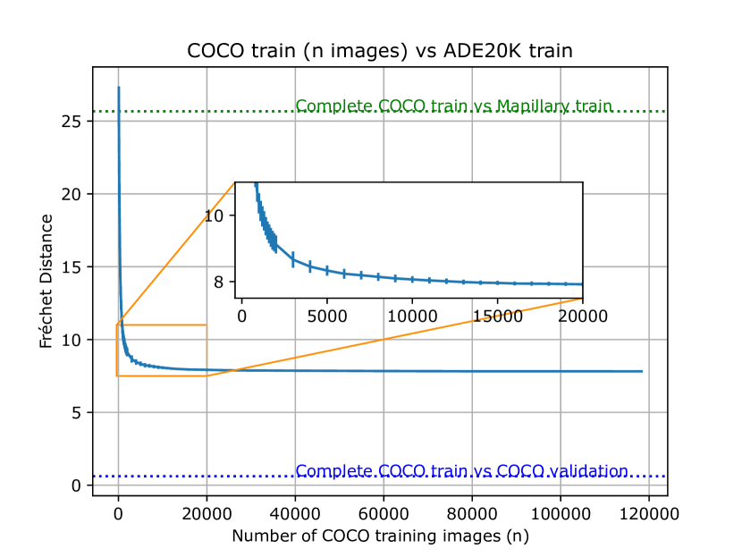
(a) Fréchet Distance (fd)

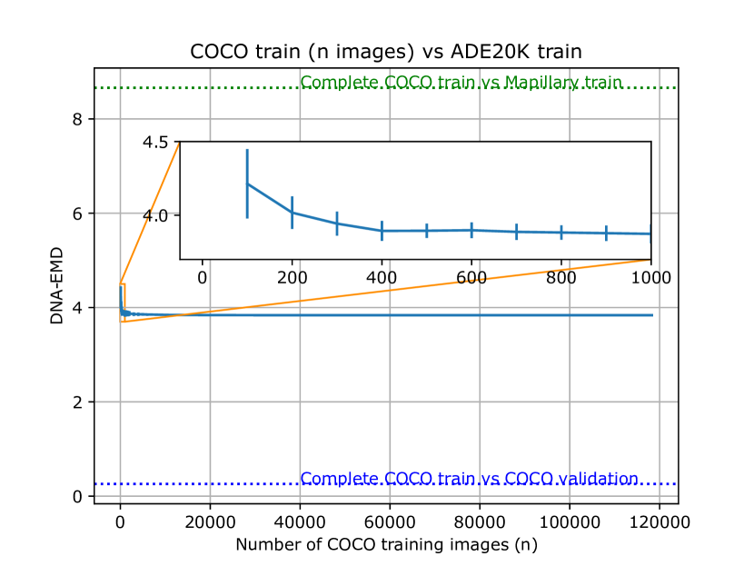
(b) Ours (dna-emd)

Figure 5: Influence of the number of images on dataset distances using DINO (ViT-B/16) features. dna-emd requires significantly fewer samples than fd from the COCO training set to reach a steady value when compared with ADE20K’s training set. Here, the distances using all images are non-zero, as there is a domain shift between the datasets. Dashed lines illustrate the distances obtained comparing COCO’s training set to its validation set and to ADE20K to illustrate the scale of the error. Results are averaged over ten seeds, with vertical lines showing the standard deviations.

5.2 Number of images required for dataset DNAs

fd is known to work poorly with scarce data [1]. We assess this in Fig. 5, comparing the distance between the entire ADE20K training set [66] and increasingly larger subsets of COCO’s training set [33]. Here, fd reaches a steady value after 10000 samples while dna-emd needs only 400, making it a reliable representation even for small datasets.

5.3 Ignoring specific attributes

Here, we demonstrate the granularity provided by individual neurons by considering: given DNAs of two datasets, can we measure the distance between them while ignoring contributions due to specifically-selected attributes?

Attribute datasets For this experiment, we split the CelebA training set according to each of the 40 labelled attributes, e.g. smiling or wearing a hat, where $A$ is the set of all attributes. We use the “in the wild” version of images which are not cropped and aligned around faces, allowing us to assess robustness to different locations and scales of attributes. Considering one attribute $a\in A$, we compute two DNAs, $\mathcal{D}_{a}$, with images with the attribute, and $\mathcal{D}_{\bar{a}}$, with images without the attribute. Neurons whose distributions vary greatly between these DNAs– i.e. are sensitive – correlate with the attribute.

Learned sensitivity removal and deviation We input the neuron-wise (for dna-fd and dna-emd) or layer-wise (for fd) distances between $\mathcal{D}_{a}$ and $\mathcal{D}_{\bar{a}}$ into a linear layer, which produces a weighted distance with which we can ignore differences of a specific attribute while maintaining sensitivity to the other attributes. Its parameters correspond to the weights $W$ for the linear combination in Eq. 5. Next, we define the sensitivity deviation of attribute $a$. For dna-emd:

$$\Delta_{a}=1-\frac{\text{EMD}_{W}(\mathcal{D}_{a},\mathcal{D}_{\bar{a}})}{\text{EMD}_{\text{avg}}(\mathcal{D}_{a},\mathcal{D}_{\bar{a}})}$$ (6)

This and all the following calculations can be applied to fd and dna-fd with the FD. If $a$ is the only attribute that changes between $\mathcal{D}_{a}$ and $\mathcal{D}_{\bar{a}}$, and $W$ is optimised to ignore $a$, then the $\text{EMD}_{W}$ should not be sensitive to $a$ and $\text{EMD}_{W}(\mathcal{D}_{a},\mathcal{D}_{\bar{a}})=0$, $\Delta_{a}=1$. For instance, we have datasets at night and datasets at day but want to compare only considering the types of vehicles present. For attributes to which we want the distance to remain sensitive, $b\in A\setminus a$, we can also measure deviations from the original distance caused by the weights $W$ using $|\Delta_{b}|$, indicating the change in sensitivity of the distance to this attribute. We want no deviation for these attributes, i.e. $|\Delta_{b}|=0$. Finally, we impose (and back-propagate, using Adam [28]) a loss:

$$L_{a}=|1-\Delta_{a}|+\frac{1}{|A|-1}\sum_{b\in{}A\setminus{}a}|\Delta_{b}|$$ (7)

meaning that we will optimise $W$ to desensitize the $\text{EMD}_{W}$ to $a$ but remain sensitive to all other attributes in $b\in A\setminus a$.

CelebA sensitivities Tab. 2 presents results as averaged over all attributes (i.e. with $a=\mathtt{hat}$ and $b$ being all other attributes, then $a=\mathtt{glasses}$ and $b$ all others, etc.). The results clearly show that neuron granularity is crucial for success as fd, which operates layer-wise, falls short against dna-emd and dna-fd. Averaged over all attributes, our approach can discard $95.5\%$ of the distance over the attributes on which we remove sensitivity, while only causing a $9.6\%$ of deviation in distances over other attributes. dna-emd performs slightly better than dna-fd, but both do very well. We observe that all feature extractors considered can somewhat succeed at the task, including the ResNet-50 with random weights, which we expect to still produce valuable features [45]. However, we obtain the best results using self-supervised models which are likely to produce more informative features.

Finding similar images Qualitatively, we expect neurons to react to general and consistent features, which should also apply to comparing image pairs and different datasets. To verify this, we compare image pairs from a different dataset, FFHQ [26], with and without specific attributes (eyeglasses and wearing hat) and select the neuron(s) with the highest dna-emd sensitivity on CelebA. Using the selected neurons, we compare the DNA${}^{\text{hist.}}$ of a selected reference image to DNAs${}^{\text{hist.}}$ of 2000 random FFHQ samples. We present our results in  Fig. 6. We can verify that very few neurons are required to focus on high-level semantic attributes, even when selected on a different dataset. We still observe some errors, possibly due to neurons reacting to several attributes simultaneously.

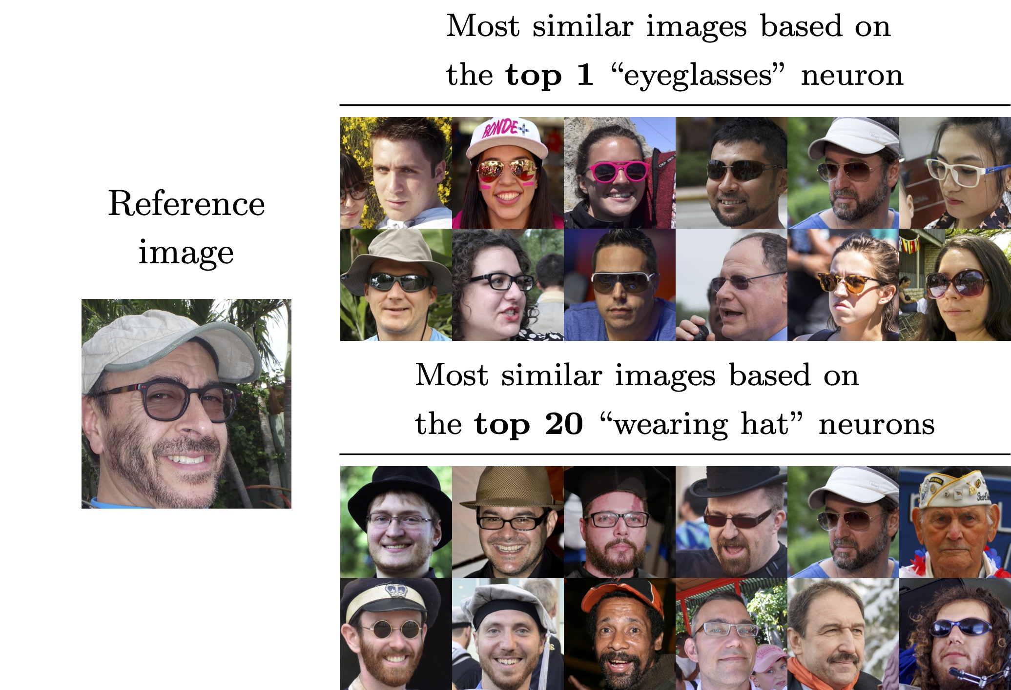
Figure 6: We seek to find the closest match to a reference image, on the left, from FFHQ, according to specific attributes – here, wearing hat and eyeglasses. To do so, we select the neurons with the highest attribute sensitivity from CelebA and use them for comparisons in FFHQ, demonstrating the generalisability of these neurons. We show that very few neurons suffice to recover images with eyeglasses and wearing hat.

Feature extractor	Mean target attribute $a$ sensitivity removal $\Delta_{a}$ (%) $\nearrow$			Mean other attributes sensitivity deviation $\frac{1}{|A|-1}\sum_{b\in{}A\setminus{}a}|\Delta_{b}|$(%) $\searrow$
	Fréchet Distance	DNA-Fréchet Distance	DNA-EMD	Fréchet Distance	DNA-Fréchet Distance	DNA-EMD
Inception-v3 [55]	9.6	94.8	92.3	9.1	11.9	10.9
CLIP image encoder (ViT-B/16) [44]	20.1	93.7	94.3	17.6	7.2	7.4
Stable Diffusion v1.4 encoder [47]	-	87.7	81.4	-	19.4	19.3
Random weights (ResNet-50) [45]	11.6	72.1	83.4	10.1	33.0	20.1
DINO (ResNet-50) [7]	15.8	87.3	93.5	8.9	16.2	9.4
DINO (ViT-B/16) [7]	19.0	93.9	94.2	16.3	10.2	9.6
Mugs (ViT-B/16) [67]	20.0	93.7	95.5	16.7	10.3	9.6
Mugs (ViT-L/16) [67]	34.6	93.3	95.3	28.0	9.4	9.1
Mean	18.7	89.6	91.2	15.2	14.7	11.9

Table 2: Customising different dataset comparison techniques to be insensitive to specific attributes. For each of the 40 attributes in CelebA, we use a weighted combination of distances over different layers or neurons with weights optimised such that the resulting distance between images with and without the attribute becomes zero. This is captured in the “target attribute sensitivity removal”, which measures the relative drop in distance. We must ensure that the distance remains sensitive to the other 39 attributes. The “other attributes sensitivity deviation” measures the relative deviation in the original distance caused by the customisation. We show averages over all attributes on the CelebA testing set. fd can only combine distances over individual layers, making it challenging to ignore some attributes while preserving others. On the other hand, neuron-wise metrics such as dna-fd and dna-emd provide sufficient granularity for customising the distance to ignore one attribute while preserving the others. We only consider the latent space of Stable Diffusion v1.4, which we treat as a single layer – hence we cannot perform a weighted combination of layers for the fd approach.

5.4 Synthetic Data

Related systems have been used in the evaluation of synthetic image-creation techniques. We thus qualitatively investigate the use of dna-emd to evaluate the quality – i.e. closeness to the distribution of real images – of StyleGANv2 [27] generated images. Here, we collect the DNAs${}^{\text{hist.}}$ for the datasets of real and generated images containing various classes [27, 63, 26]. We use these to select the most sensitive neurons (as above in Fig. 6) to differences between real and fake images, which we expect to be good indicators of realism. These neurons are used to compare a separate dataset with generated images of one class not included in the datasets responsible for neuron selection – e.g. when evaluating realism for cars, we select neurons based on cats, horses, churches, and faces, focusing on general realism rather than car-specific features.

Our results are reported in Fig. 7. We clearly identify outliers in the generated samples using either selected or all neurons. However, when using all neurons, top matches do not always match our perceptual quality assessment. By selecting a small number of neurons reacting to realism, we favour images with fewer synthetic generation artefacts.

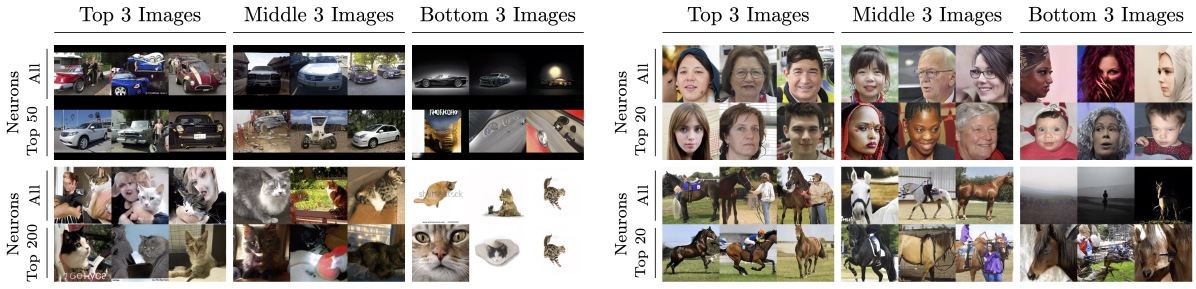
Figure 7: Generated StyleGANv2 [27] images of cars, faces, cats, and horses, ranked by dna-emd similarity to the corresponding real dataset’s DNA${}^{\text{hist.}}$. We selected neurons for realism by comparing real and synthetic images only featuring other classes (for general realism rather than focusing on class-specific differences) and compared this to using all neurons. Generally, selecting neurons results in rankings that better align with perceptual quality.

5.5 Generalisation prediction under domain shifts

Above, we have compared images and datasets from similar domains. However, many applications require comparing datasets from distinct domains. Here, we show the power of DNAs in cross-dataset generalisation prediction, which can serve, for instance, to select the best dataset for training when performing transfer learning.

For this, we compare our ranking of distances from dataset DNAs to the measured cross-dataset generalisation of a semantic-segmentation network reported in Tab. 3 of Lambert et al. [31]. This reference provides mIoUs from an HRNet-W48 [58] semantic segmentation model architecture trained on seven datasets: ADE20K [66], COCO [33], BDD100K[62], Cityscapes[9], IDD [57], Mapillary [38], and SUN-RGBD [53], and evaluated on all seven corresponding validation sets. Cross-generalization varies widely for different pairs of datasets, with mIoUs ranging from 0.2 (training on Cityscapes and validating on SUN-RGBD) to 69.7 (training on Mapillary and validating on Cityscapes). Therefore, for each validation set $v\in V$, we have a ranking of which dataset’s training sets transferred best in terms of mIoU. We denote by $T^{\text{gt}}_{v}[i]$ the training set used by the model producing the $i$-th highest mIoU for validation set $v$, and by $\text{mIoU}_{v}(t)$ the mIoU observed with a model trained on $t$ and evaluated on the validation set $v$.

A good dataset distance metric will produce similar mIoU rankings – and importantly, without training a model. We therefore compare all pairs of datasets using fd, dna-fd, and dna-emd, and rank them by distance. We denote by $T_{v}^{\text{pred}}[i]$ the training set ranked at the $i$-th position when compared to validation set $v$. To aggregate results, we measure the discrepancy $d$ between predicted and reference rankings using average mIoU differences:

$$d=\frac{1}{|V||T|}\sum_{v\in V}\sum_{i=1}^{|T^{\text{gt}}_{v}|}|\text{\footnotesize mIoU}_{v}(T_{v}^{\text{gt}}[i])-\text{\footnotesize mIoU}_{v}(T_{v}^{\text{pred}}[i])|$$ (8)

This discrepancy penalises out-of-rank predictions based on the difference of mIoU at those ranks.

In addition to the Mugs feature extractor, we also consider domain-specific feature extractors. We evaluate cross-dataset generalisation using features extracted from an HRNet-W48 semantic segmentation model trained on MSeg [31] which combines all datasets used in the experiment. We also use HRNet-W48 models trained on the validation domains. We report results relying on the features from the last layer of each model. We present the summary results for different feature extractors and metrics in Tab. 3.

Using dna-emd with a self-supervised network provides the best cross-dataset generalization. While being specifically adapted to the task and datasets considered, HRNet-W48 models fail to perform as well, likely due to the less general features not allowing to measure domain shifts as well. The average mIoU error in ranking datasets with dna-emd with Mugs features is only 0.76, indicating very good predictions of cross-generalization performance without training a model, markedly superior to fd and dna-fd.

Feature extractor	Fréchet Distance	DNA-Fréchet Distance	DNA-EMD
Mugs (ViT-B/16)	1.66	1.79	0.76
HRNet-W48 (all domains)	9.63	11.18	9.40
HRNet-W48 (val. domain)	13.9	14.5	6.85
Random ordering	14.93 $\pm$ 1.86 (50 samples)

Table 3: Effectiveness of using dataset comparisons to predict semantic segmentation transfer learning performance. We compare the ranking of training datasets by a model’s transfer learning performance to the ranking of datasets based on their distance to the validation set. We measure the severity of errors in predicted ranking by calculating the average difference in mIoU scores of reference models when ranked by mIoU and when ranked by the distance between their training and validation sets.

6 Limitations

Labelled data requirements for neuron selection Our neuron selection experiments in this work rely on labelled images to find neuron combination strategies. This is not always available, in which case unsupervised clustering techniques such as deepPIC [23] could be used.

Combining neurons Many neurons are likely to be polysemantic [12, 39], meaning that they are likely to react to multiple unrelated inputs. The approaches used in this paper to combine information from different neurons might be too limited to properly isolate specific attributes.

Discarded information in the DNA representation To make DNAs practical and scalable, we have discarded information about features. This includes spatial information about where activations occur and dependencies between activations of all neurons. These could help to obtain an even better representation.

7 Conclusion

We have presented a general and granular representation for images. This representation is based on keeping track of distributions of neuron activations of a pre-trained feature extractor. One DNA can be created from a single image or a complete dataset. Image DNAs are compact and granular representations which require no training, hyperparameter tuning, or labelling, regardless of the type of images considered. Our experiments have demonstrated that even with simplistic comparison strategies, DNAs can provide valuable insights into attribute-based comparisons, synthetic image quality assessment, and dataset differences.

Appendix A Technical details

A.1 Feature extractors

A.1.1 Features considered

We present details of the locations of neurons considered in Sec. A.1.1. For the Stable diffusion v1.4 encoder, we expect the latent space to contain sufficient information to reconstruct the original image. As such, we only consider the latent space, treating each element as a neuron.

Feature extractor architecture	Layers considered	Number of neurons per layer
Inception-v3	Outputs of the first and second max pooling layers, input features to the auxiliary classifier, and output of the final average pooling layer	$64$ / $192$ / $768$ / $2048$
Stable diffusion v1.4 encoder	Latent space produced by the VAE encoder	$4096$
ResNet-50	Output of each block	$3\times[256]$ / $4\times[512]$ /
		$6\times[1024]$ / $3\times[2048]$
Vision Transformer (ViT-B/16)	Output of each of the 12 self-attention layers, and output of the final normalisation layer	$13\times[768]$
Vision Transformer (ViT-L/16)	Output of each of the 24 self-attention layers, and output of the final normalisation layer	$25\times[1024]$
HRNet-W48	Outputs of each stage, where we treat each branch of the stage as providing a different layer. We also include the output of the classifier	$256$ / $(48/96)$ / $(48/96/192)$ /
		$(48/96/192/384)$ / $194$

Table 4: Details of layers and neurons considered for all architectures.

A.1.2 Spatial accumulation for Vision Transformers

In Sec. 3.2, we describe feature maps as having spatial dimensions $S_{h}^{l}\times S_{w}^{l}$. In the case of vision transformers, we treat the patch/token dimensions as the only spatial dimension. Activations over the patch/token dimension are accumulated in the histogram of the corresponding neuron.

A.2 Data processing

Activation normalisation

As discussed in Fig. 4, activations at each neuron are normalised to ensure comparable scales over different neurons. The normalisation relies on tracking minimum and maximum activation values over the following datasets: StyleGANv2 generated images of cars, cats, churches, faces, and horses, LSUN cars, LSUN cats, LSUN churches, LSUN horses, FFHQ, Metfaces, CelebA, Cityscapes, KITTI, IDD, ADE20K, BDD100K, Mapillary, Wilddash, COCO, and SUN-RGBD. Using the minimum and maximum values observed, $\mathtt{a}_{\text{min}}$ and $\mathtt{a}_{\text{max}}$, for each neuron over all of these datasets, we recompute normalised activations $\mathtt{a}_{\text{norm}}$ from the activations observed during inference $\mathtt{a}$ to produce histograms as follows:

$$\mu=\frac{1}{2}(\mathtt{a}_{\text{max}}+\mathtt{a}_{\text{min}})$$ (9)

$$\sigma=\frac{1}{2}(\mathtt{a}_{\text{max}}-\mathtt{a}_{\text{min}})$$ (10)

$$\mathtt{a}_{\text{norm}}=\frac{\mathtt{a}-\mu}{\sigma}$$ (11)

Cropping

Images are centre-cropped to squares and resized depending on the feature extractor, as described in Tab. 5.

Feature extractor	Image size used
Inception-v3	$299\times 299$
CLIP image encoder (ViT-B/16)	$224\times 224$
Stable diffusion v1.4 encoder	$256\times 256$
Random weights (ResNet-50)	$224\times 224$
DINO (ResNet-50)	$224\times 224$
DINO (ViT-B/16)	$224\times 224$
Mugs (ViT-B/16)	$224\times 224$
Mugs (ViT-L/16)	$224\times 224$
HRNet-W48	$360\times 360$

Table 5: Image sizes used for different feature extractors.

A.3 Random image transformations for Cityscapes retrieval task

In Sec. 5.1, we attempt to retrieve randomly augmented Cityscapes images. The augmentations applied to each image are 2 randomly selected operations applied sequentially. The operations considered are Identity, Shear X, Shear Y, Translate X, Translate Y, Rotate, Adjust brightness, Adjust saturation, Adjust contrast, Adjust sharpness, Posterize, Auto contrast, Equalize, Salt-and-pepper noise, Gaussian noise, and Blur.

A.4 Weights optimisation for attribute removal

For the optimisation of weights used in Sec. 5.3, we use the Adam optimiser with a learning rate of $1\mathrm{e}{-5}$, and first- and second-moment decays rates $\beta_{1}=0.9$ and $\beta_{2}=0.999$. Weights are initialised to a constant value of $\frac{1}{\text{number of neurons}}$.

We perform optimisation of the loss in Eq. 7 on DNAs from the training set, which were generated using up to $50000$ images for each DNA. We use early stopping by monitoring the loss on the validation set, stopping after $50$ iterations without improvements. The results in Tab. 2 are then reported on the testing set.

A.5 Neuron selection for StyleGANv2 synthetic images

In Sec. 5.4, we select neurons to rank images from one class by selecting the most sensitive neurons to differences between real and fake images of all other classes. More precisely, this is done by creating a DNA${}^{\text{hist.}}$ representing all real images from the other classes, and a DNA representing all fake images from the other classes. Combining the DNA${}^{\text{hist.}}$ of multiple datasets is done by summing the counts for each histogram from the DNAs${}^{\text{hist.}}$ to combine. This is equivalent to creating a new single DNA${}^{\text{hist.}}$ using all the images from the different datasets. The sensitivity of neurons is then computed using the neuron-wise EMD between the combined real DNA${}^{\text{hist.}}$ and the combined fake DNA${}^{\text{hist.}}$.

A.6 Example histograms

In Secs. A.1.1 and A.1.1, we present examples of histograms from specific neurons of the DNA${}^{\text{hist.}}$ of CelebA images with or without some attributes. We observe that their shapes would not always be well approximated by a Gaussian distribution, as is done with DNAs${}^{\text{Gauss.}}$.

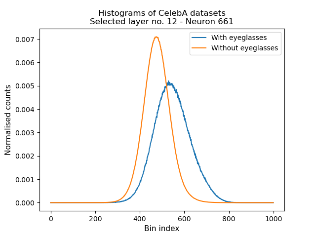
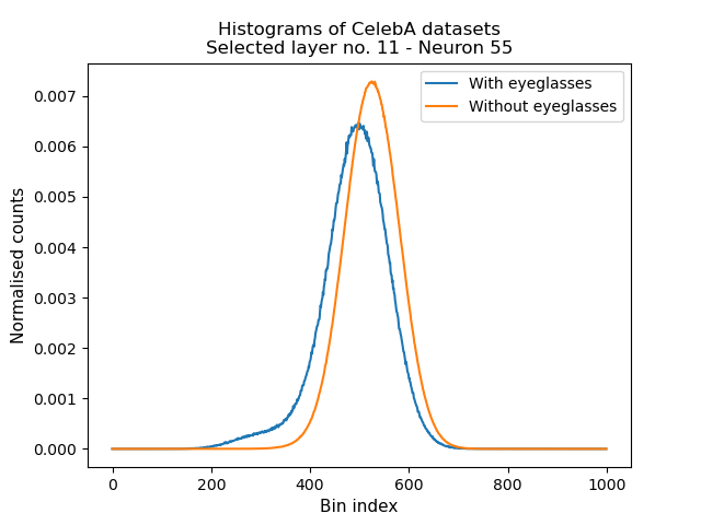
(a) Examples of histograms resulting in the largest Earth Mover’s Distances

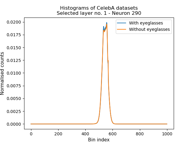
(b) Examples of histograms resulting in the lowest Earth Mover’s Distances

Figure 8: Visualisation of normalised histograms for specific neurons from DNAs${}^{\text{hist.}}$ (Mugs ViT-B/16) of images from the CelebA dataset with and without eyeglasses.

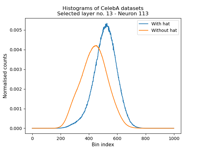
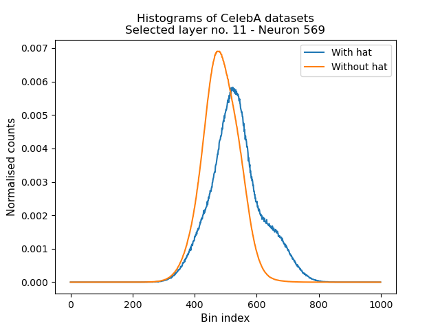
(a) Examples of histograms resulting in the largest Earth Mover’s Distances

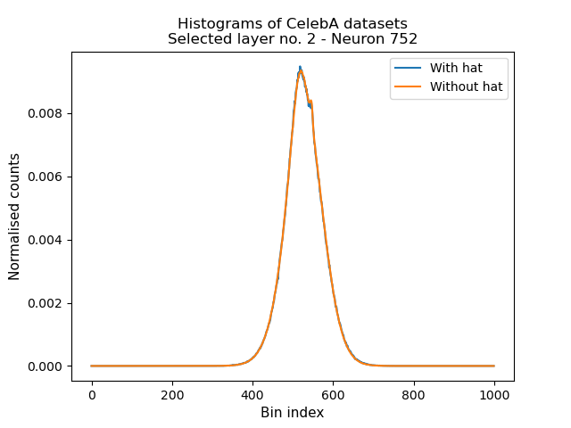
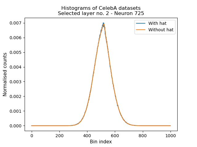
(b) Examples of histograms resulting in the lowest Earth Mover’s Distances

Figure 9: Visualisation of normalised histograms for specific neurons from DNAs${}^{\text{hist.}}$ (Mugs ViT-B/16) of images from the CelebA dataset with and without wearing hat.

Appendix B Additional results details

The following sections present more detailed results. Unless mentioned otherwise, the results use dna-emd with a Mugs (ViT-B/16) feature extractor.

B.1 Comparing images to a reference dataset with different neurons

In Sec. A.1.1, we present ranked images from different datasets with specific neurons from their DNAs${}^{\text{hist.}}$ compared to the DNA${}^{\text{hist.}}$ of the Cityscapes dataset. Compared to Fig. 4 in which all neurons are considered, here we show results with neurons from the first and last selected layers of the feature extractor.

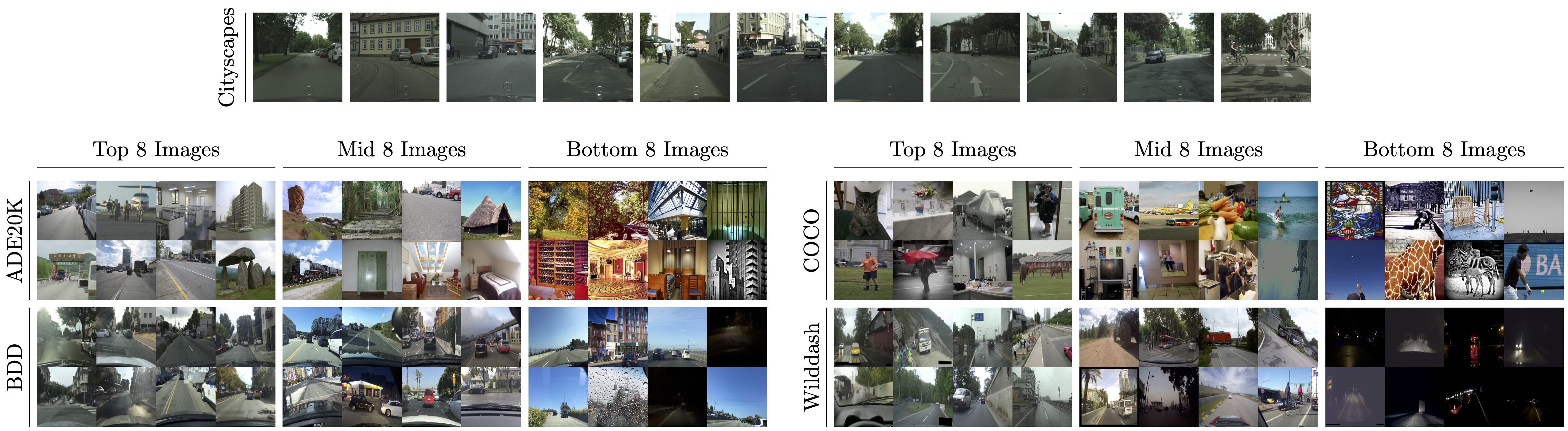
(a) Using all neurons from the first layer of the Mugs (ViT-B/16) feature extractor.

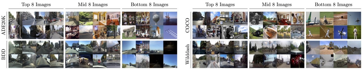
(b) Using all neurons from the last layer of the Mugs (ViT-B/16) feature extractor.

Figure 10: Images from different datasets organised by dna-emd when compared to Cityscapes [9] using different neurons from the feature extractor.

When using neurons from the first layer, colours and textures appear much more important in producing the score. The best matches sometimes do not correspond to similar types of scenes, such as in COCO, but display similar colour profiles. Worst matches tend to contain high-frequency patterns or few features. On the other hand, when using neurons from the last layer, semantic content seems to be the main factor. Top-ranking images always show the same type of environment but do not always have the same colour profiles.

B.2 CelebA attribute sensitivity removal

B.2.1 Visualisation of dna-emd neuron-wise differences and weights learned

In Sec. A.1.1, we compare the neuron-wise EMD between DNAs${}^{\text{hist.}}$ of datasets with and without specific attributes to the weights learned in Sec. 5.3.

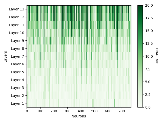
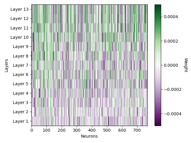
(a) Distances (left) and optimised weights (right) for the eyeglasses attribute.

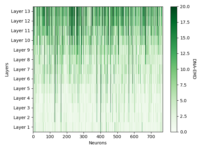
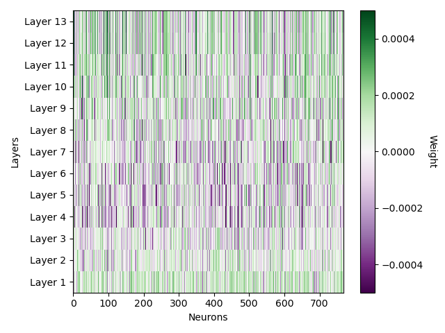
(b) Distances (left) and optimised weights (right) for the wearing hat attribute.

Figure 11: Comparison of dna-emd distances between DNAs${}^{\text{hist.}}$ with and without an attribute, and optimised weights for attribute removal.

Distances appear larger at later layers, but the attention from the weights allows us to focus on specific neurons spread over all layers and thus ignore the attribute, highlighting the need for granularity and a multi-layered approach.

B.2.2 Standard deviations of scores

Tab. 6 details the standard deviations computed over all forty attributes for the results in Tab. 2 in Sec. 5.3.

Feature extractor	Target attribute sensitivity removal $\Delta_{\text{rem}}$ std. dev. (%)			Other attributes sensitivity deviation $|\Delta_{\text{rem}}|$ std. dev. (%)
	Fréchet Distance	DNA-Fréchet Distance	DNA-EMD	Fréchet Distance	DNA-Fréchet Distance	DNA-EMD
Inception-v3 [55]	7.55	4.30	5.65	7.40	6.99	6.37
CLIP image encoder (ViT-B/16) [44]	13.84	5.78	4.90	12.80	4.24	3.59
Stable Diffusion v1.4 encoder [47]	-	9.62	11.05	-	6.83	6.32
Random weights (ResNet-50) [45]	12.13	28.05	19.58	11.91	17.12	9.97
DINO (ResNet-50) [7]	13.03	13.28	5.19	6.91	9.72	4.34
DINO (ViT-B/16) [7]	12.26	4.50	4.19	12.47	5.62	4.83
Mugs (ViT-B/16) [67]	12.18	5.47	4.76	11.62	6.33	5.39
Mugs (ViT-L/16) [67]	17.89	5.18	4.28	16.91	5.71	4.62

Table 6: Standard deviations over all forty attributes for scores presented in Tab. 2.

B.2.3 Detailed deviations

In Sec. 5.3, we weighted distances over different neurons to remove sensitivity to one attribute while preserving others. In Fig. 12, we visualise which attributes deviate most when ignoring another.

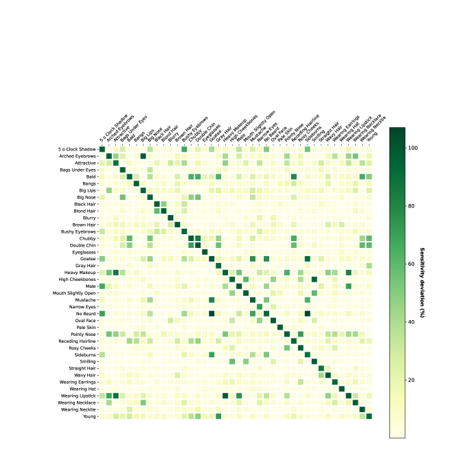
Figure 12: For each ignored attribute in the rows, we show the sensitivity deviation of all other attributes from the columns. The diagonals describe the relative drop in distances on the ignored attribute.

We see that some attributes are particularly challenging to disentangle, often when we expect them to be correlated. For example, when ignoring the no beard attribute, we cause a large deviation in the goatee attribute. We might expect these to react to similar neurons. Still, we believe improvements in the optimised loss might help reduce this entanglement.

We also visualise overlaps between attributes in the CelebA dataset in Fig. 13.

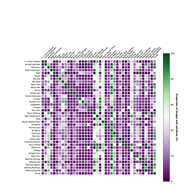
Figure 13: Illustration of correlations between attributes in the CelebA dataset. For each attribute in the rows, we show the percentage of images containing that attribute that also possess the attribute in the columns. Attributes can be negatively correlated when we observe values close to $0\%$, or positively correlated with values close to $100\%$.

B.3 FFHQ image pair comparisons

In this section, we present additional details for the results shown in Fig. 6. In addition to showing middle and bottom-ranked matches, we also consider different neurons for comparisons. Fig. 14 presents the matches ranked using all neurons from different layers of the feature extractor.

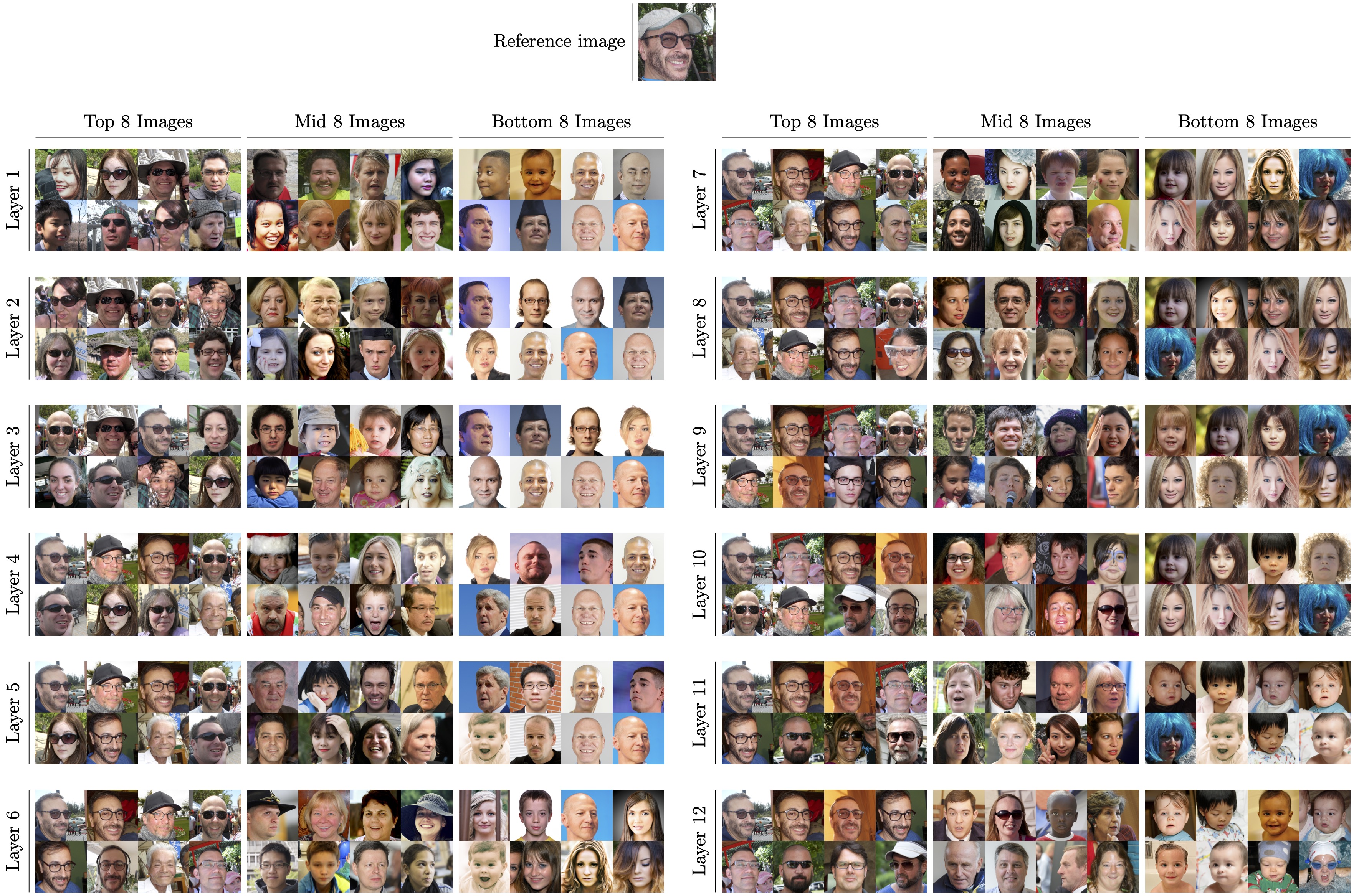
Figure 14: Ranked matches to the reference image using dna-emd with neurons from different layers of the Mugs (ViT-B/16) feature extractor.

Top matches from the first layer do not always focus on having similar semantic attributes. However, they all contain similar backgrounds and colours. Top matches from the last layer have much more diverse colour profiles and better match other images of the person in the reference image.

In Figs. 15 and 16, we present ranked matches using different numbers of selected neurons to focus on specific attributes. For the wearing hat attribute, we see that using too few or too many neurons can lead to not focusing on the desired attribute anymore. For the eyeglasses attribute, we are able to focus on the correct matches with all numbers of neurons. Even when using all neurons and no selection strategy, images with the attribute seem sufficiently favoured to be better ranked.

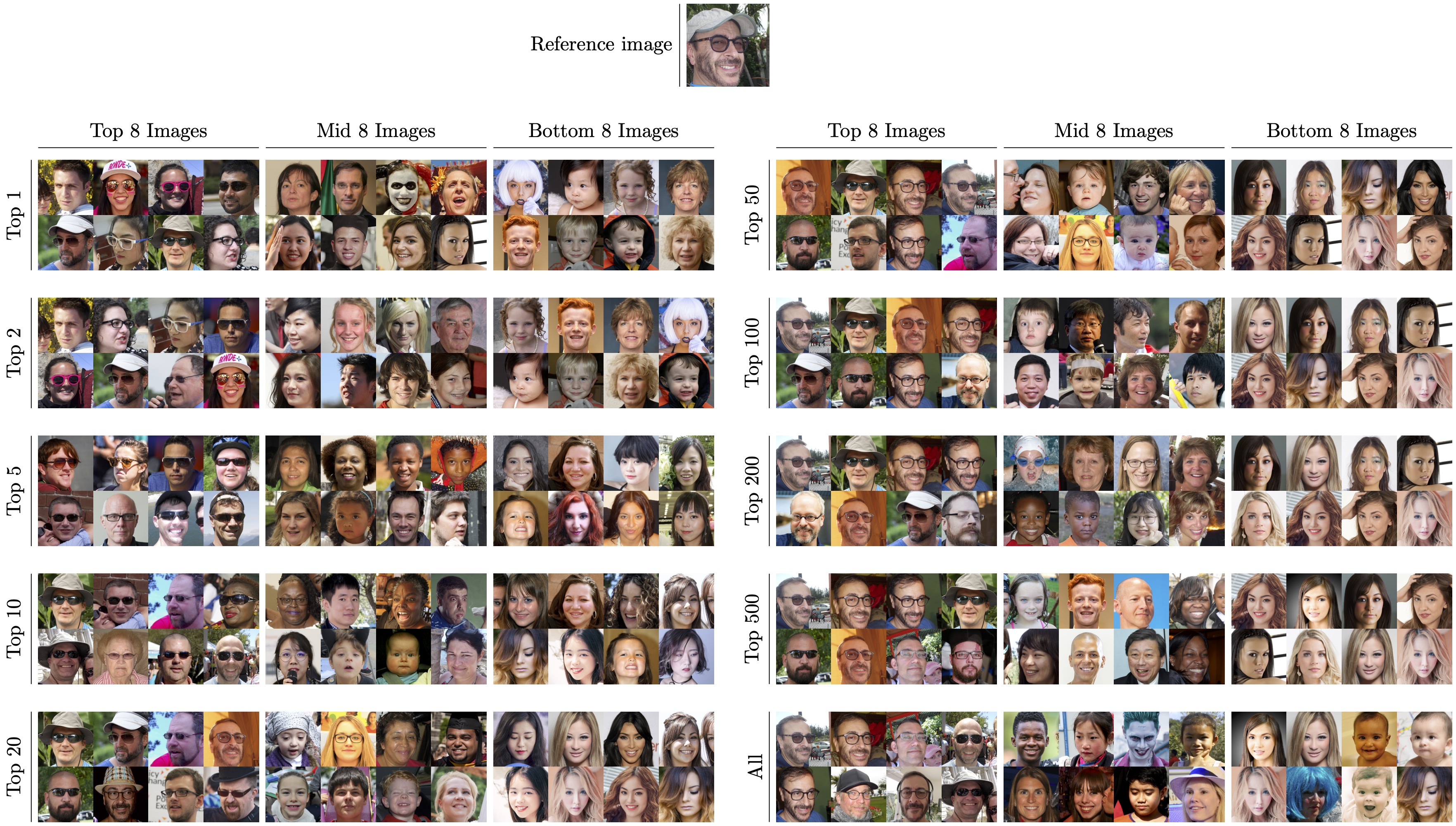
Figure 15: Ranked matches to the reference image using dna-emd with neurons of the Mugs (ViT-B/16) feature extractor sensitive to the eyeglasses attribute.

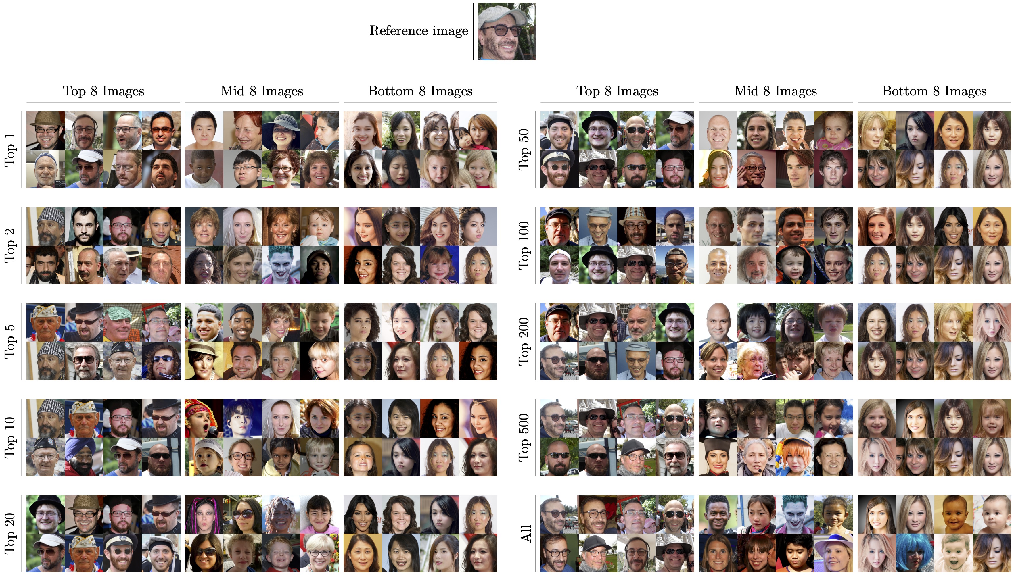
Figure 16: Ranked matches to the reference image using dna-emd with neurons of the Mugs (ViT-B/16) feature extractor sensitive to the wearing hat attribute.

B.4 StyleGANv2 ranked images

We present more results of synthetic StyleGANv2 image rankings for different numbers of selected neurons for realism in Figs. 17, 18, 19, 20 and 21.

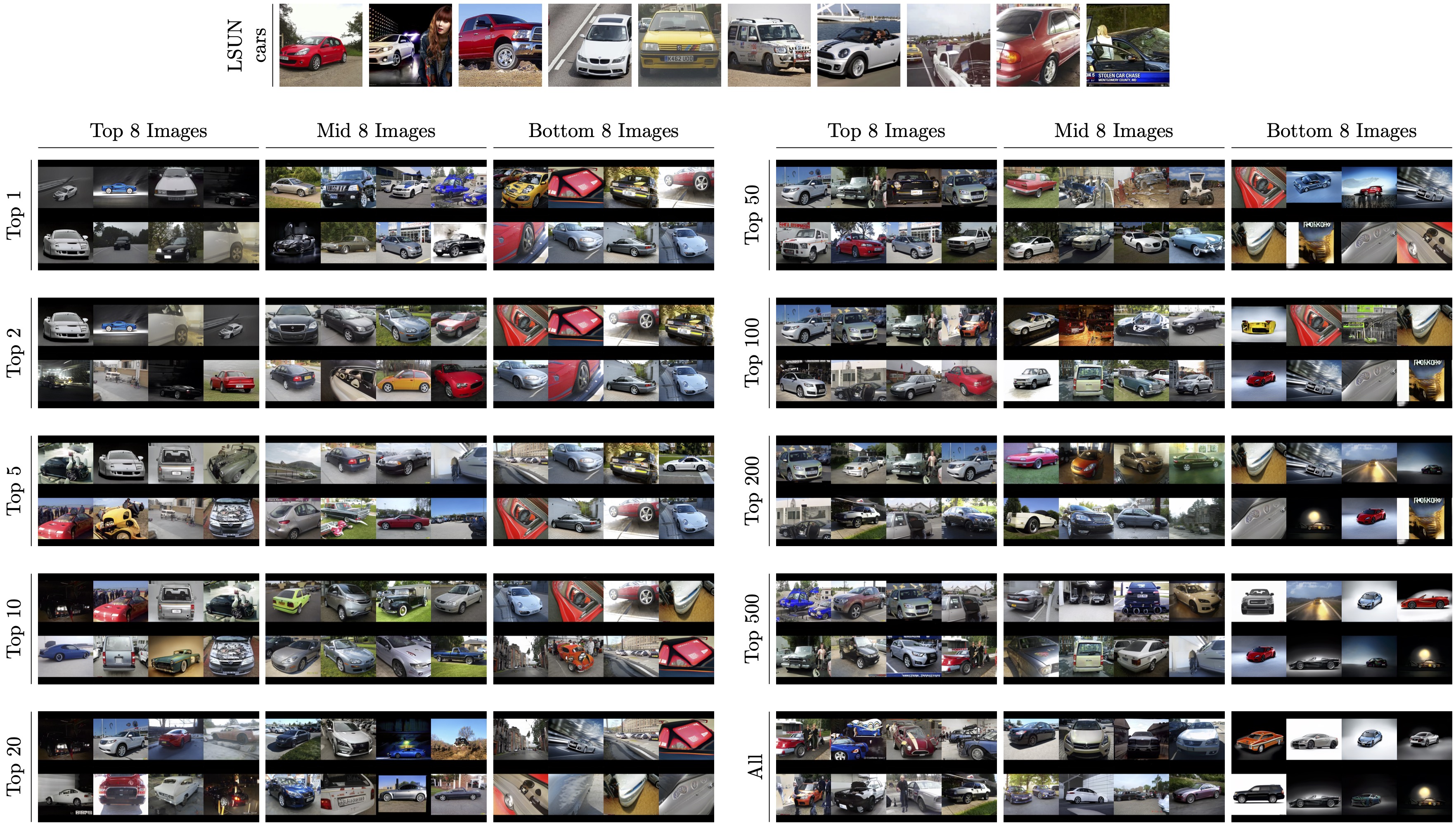
Figure 17: Generated StyleGANv2 [27] car images ranked by dna-emd when compared to the LSUN car images. We show the rankings for different numbers of selected neurons. The neuron selection strategy selects the most sensitive neurons when comparing real and synthetic images from other datasets.

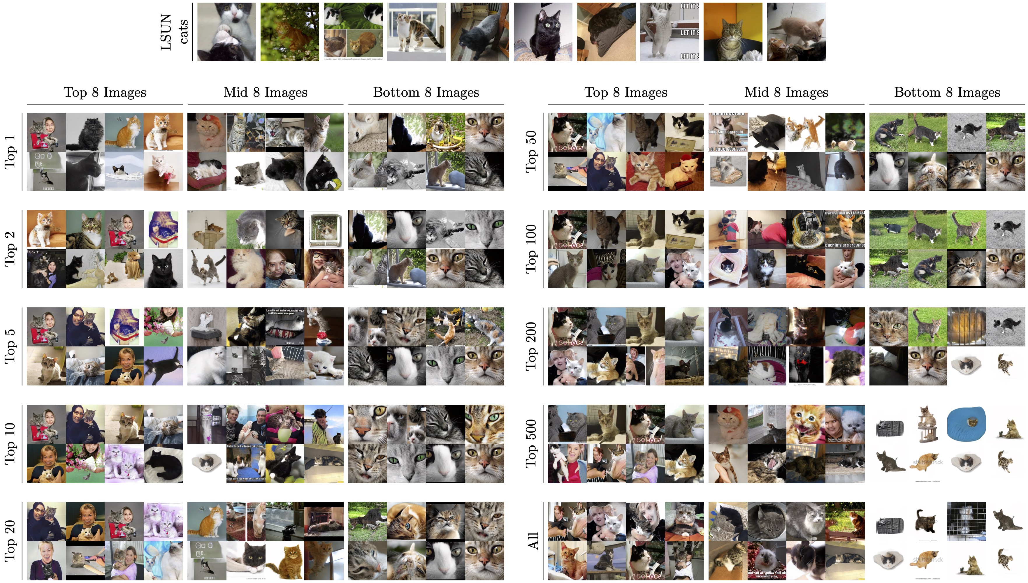
Figure 18: Generated StyleGANv2 [27] cat images ranked by dna-emd when compared to the LSUN cat images. We show the rankings for different numbers of selected neurons. The neuron selection strategy selects the most sensitive neurons when comparing real and synthetic images from other datasets.

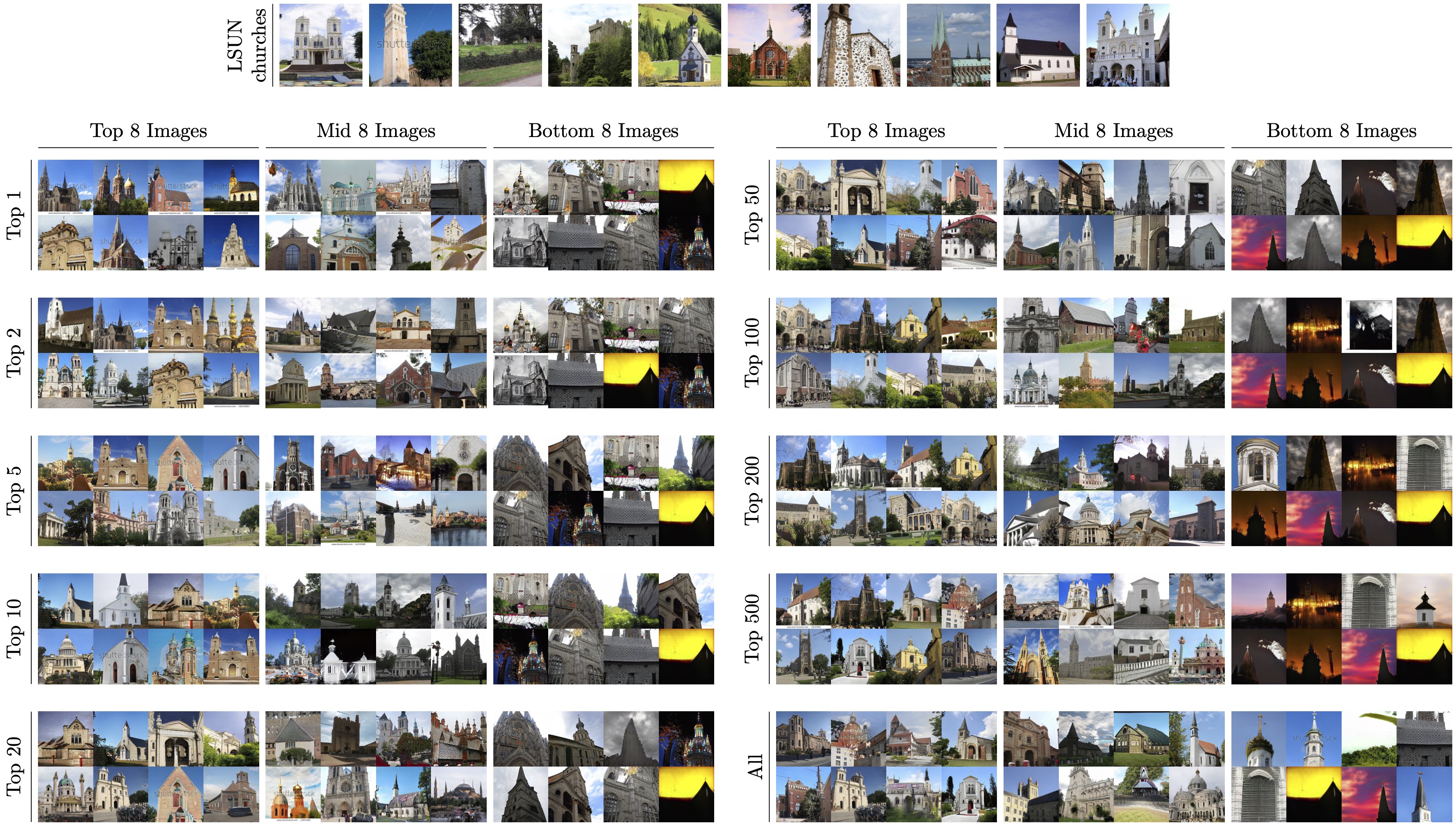
Figure 19: Generated StyleGANv2 [27] church images ranked by dna-emd when compared to the LSUN church images. We show the rankings for different numbers of selected neurons. The neuron selection strategy selects the most sensitive neurons when comparing real and synthetic images from other datasets.

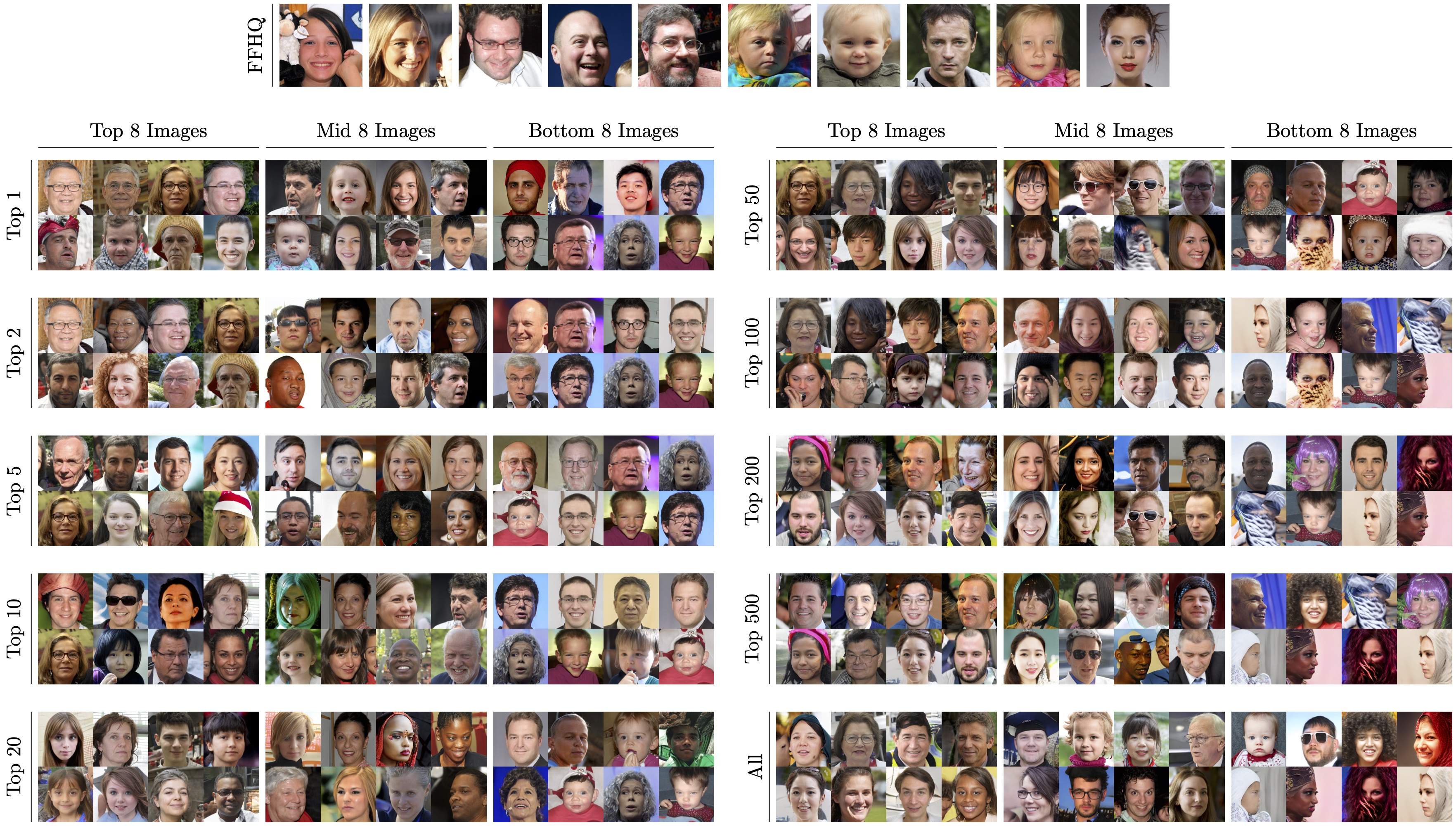
Figure 20: Generated StyleGANv2 [27] face images ranked by dna-emd when compared to the FFHQ images. We show the rankings for different numbers of selected neurons. The neuron selection strategy selects the most sensitive neurons when comparing real and synthetic images from other datasets.

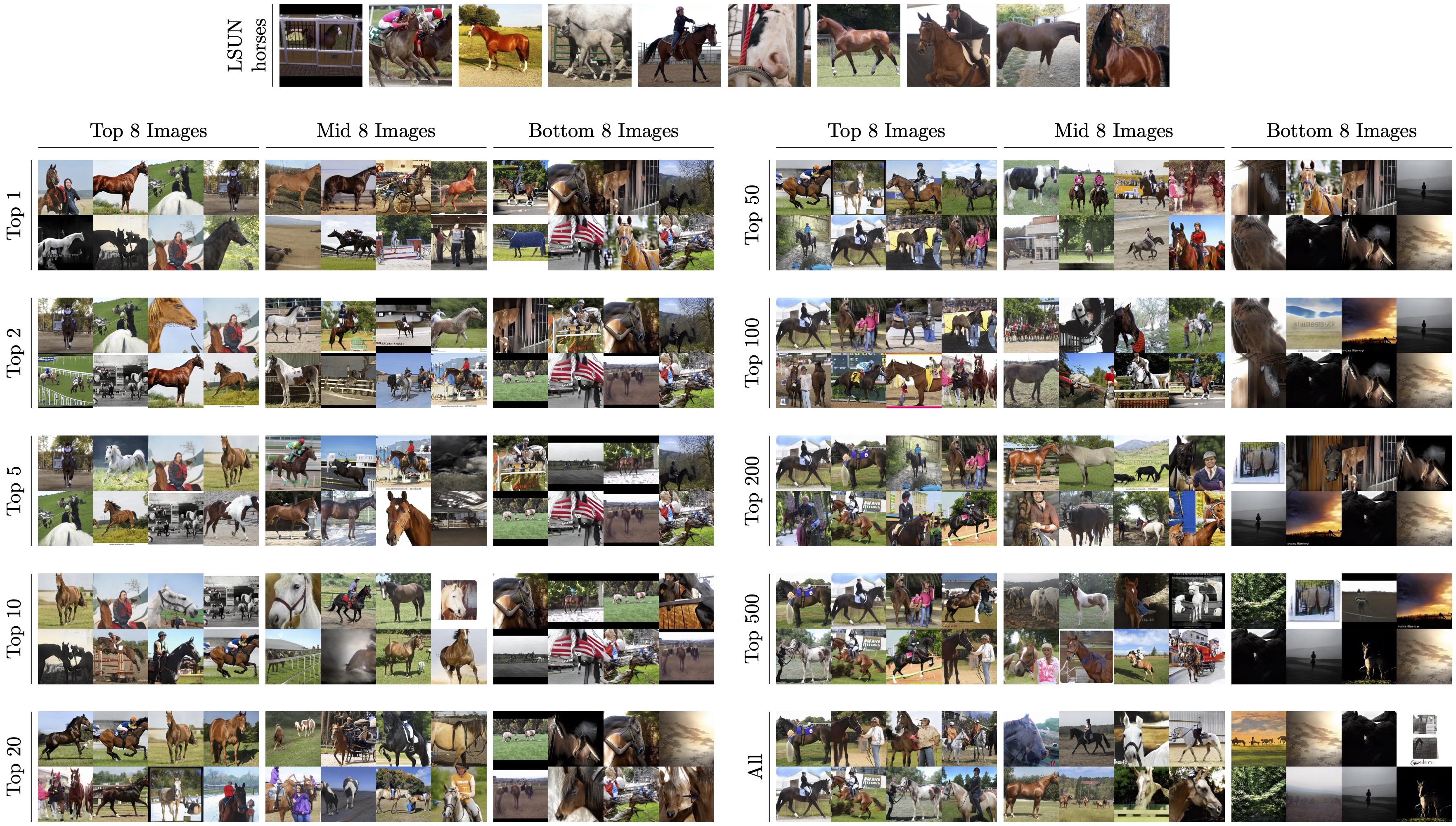
Figure 21: Generated StyleGANv2 [27] horse images ranked by dna-emd when compared to the LSUN horse images. We show the rankings for different numbers of selected neurons. The neuron selection strategy selects the most sensitive neurons when comparing real and synthetic images from other datasets.

B.5 Cross-dataset generalisation

Finally, in Tabs. 7, 8, 9, 10 and 11 we present detailed cross-dataset generalisation results that are used to produce Tab. 3. Details are provided for the HRNet-W48 and Mugs models using dna-emd, and for the Mugs model with dna-fd and fd.

	Validation datasets
	ADE20K	BDD100K	Cityscapes	COCO	IDD	Mapillary	SUN-RGBD
Training datasets	45.3 - ADE20K	63.2 - BDD100K	77.6 - Cityscapes	52.6 - COCO	64.8 - IDD	56.2 - Mapillary	43.9 - SUN-RGBD
	19.6 - COCO	60.2 - Mapillary	69.7 - Mapillary	14.5 - ADE20K	48.2 - Mapillary	26.7 - COCO	35.3 - ADE20K
	7.1 - SUN-RGBD	45.0 - Cityscapes	60.9 - BDD100K	6.7 - Mapillary	33.9 - BDD100K	24.3 - ADE20K	29.4 - COCO
	6.2 - Mapillary	44.1 - COCO	50.2 - IDD	3.7 - BDD100K	31.3 - Cityscapes	24.3 - IDD	0.6 - IDD
	4.1 - BDD100K	43.7 - IDD	46.2 - COCO	3.3 - SUN-RGBD	31.0 - COCO	24.0 - BDD100K	0.2 - BDD100K
	3.1 - Cityscapes	41.5 - ADE20K	44.3 - ADE20K	3.1 - Cityscapes	27.0 - ADE20K	22.4 - Cityscapes	0.2 - Cityscapes
	3.1 - IDD	2.2 - SUN-RGBD	2.6 - SUN-RGBD	3.1 - IDD	1.0 - SUN-RGBD	1.1 - SUN-RGBD	0.2 - Mapillary

(a) Observed cross-dataset generalisation on semantic segmentation from Lambert et al. [31] (mIoU). Each column corresponds to the evaluation of one dataset (validation set). Rows are ordered by a cross-generalisation performance from training on each dataset (training set).

	Validation datasets
	ADE20K	BDD100K	Cityscapes	COCO	IDD	Mapillary	SUN-RGBD
Training datasets	0.84 - ADE20K	3.61 - BDD100K	3.18 - Cityscapes	0.64 - COCO	4.48 - IDD	0.85 - Mapillary	2.22 - SUN-RGBD
	9.17 - COCO	8.91 - Mapillary	15.9 - Mapillary	9.2 - ADE20K	12.88 - Mapillary	9.72 - BDD100K	12.71 - ADE20K
	12.66 - SUN-RGBD	13.03 - IDD	17.13 - BDD100K	15.4 - SUN-RGBD	13.54 - BDD100K	11.52 - IDD	15.57 - COCO
	21.18 - Mapillary	17.18 - Cityscapes	17.15 - IDD	21.79 - Mapillary	18.95 - Cityscapes	16.19 - Cityscapes	26.92 - IDD
	21.57 - IDD	22.56 - ADE20K	25.61 - ADE20K	22.36 - IDD	22.53 - ADE20K	21.26 - ADE20K	27.01 - Mapillary
	22.58 - BDD100K	23.88 - COCO	25.73 - COCO	23.86 - BDD100K	23.33 - COCO	21.89 - COCO	27.96 - BDD100K
	26.17 - Cityscapes	27.96 - SUN-RGBD	30.47 - SUN-RGBD	26.41 - Cityscapes	27.51 - SUN-RGBD	26.95 - SUN-RGBD	31.08 - Cityscapes

(b) Ordered datasets ranked by dna-emd with corresponding EMD values. The EMD here is computed using the last layer of the Mugs (ViT-B/16) feature extractor.

	Validation datasets
	ADE20K	BDD100K	Cityscapes	COCO	IDD	Mapillary	SUN-RGBD
Training datasets	45.3 - ADE20K	63.2 - BDD100K	77.6 - Cityscapes	52.6 - COCO	64.8 - IDD	56.2 - Mapillary	43.9 - SUN-RGBD
	19.6 - COCO	60.2 - Mapillary	69.7 - Mapillary	14.5 - ADE20K	48.2 - Mapillary	24.0 - BDD100K	35.3 - ADE20K
	7.1 - SUN-RGBD	43.7 - IDD	60.9 - BDD100K	3.3 - SUN-RGBD	33.9 - BDD100K	24.3 - IDD	29.4 - COCO
	6.2 - Mapillary	45.0 - Cityscapes	50.2 - IDD	6.7 - Mapillary	31.3 - Cityscapes	22.4 - Cityscapes	0.6 - IDD
	3.1 - IDD	41.5 - ADE20K	44.3 - ADE20K	3.1 - IDD	27.0 - ADE20K	24.3 - ADE20K	0.2 - Mapillary
	4.1 - BDD100K	44.1 - COCO	46.2 - COCO	3.7 - BDD100K	31.0 - COCO	26.7 - COCO	0.2 - BDD100K
	3.1 - Cityscapes	2.2 - SUN-RGBD	2.6 - SUN-RGBD	3.1 - Cityscapes	1.0 - SUN-RGBD	1.1 - SUN-RGBD	0.2 - Cityscapes

(c) Ordered datasets ranked by dna-emd with corresponding mIoU values. The ranking is taken from Tab. 7(b), but we show the mIoUs for the corresponding datasets from Tab. 7(a) instead.

Validation datasets
ADE20K	BDD100K	Cityscapes	COCO	IDD	Mapillary	SUN-RGBD
0.0	0.0	0.0	0.0	0.0	0.0	0.0
0.0	0.0	0.0	0.0	0.0	2.7	0.0
0.0	1.3	0.0	3.4	0.0	0.0	0.0
0.0	0.9	0.0	3.0	0.0	1.9	0.0
1.0	2.2	1.9	0.2	4.0	0.3	0.0
1.0	2.6	1.9	0.6	4.0	4.3	0.0
0.0	0.0	0.0	0.0	0.0	0.0	0.0
Average absolute mIoU difference: 0.76

(d) Differences between the mIoUs of the reference ranking (Tab. 7(a)) and the mIoUs for the predicted dna-emd ranking (Tab. 7(c)).

Table 7: Detailed results comparing the observed cross-dataset generalisation of the HRNet-W48 semantic segmentation models to predictions relying only on datasets using dna-emd with the Mugs (ViT-B/16) feature extractor. The final value reported in Tab. 3 corresponds to the average of the values in Tab. 7(d).

	Validation datasets
	ADE20K	BDD100K	Cityscapes	COCO	IDD	Mapillary	SUN-RGBD
Training datasets	45.3 - ADE20K	63.2 - BDD100K	77.6 - Cityscapes	52.6 - COCO	64.8 - IDD	56.2 - Mapillary	43.9 - SUN-RGBD
	19.6 - COCO	60.2 - Mapillary	69.7 - Mapillary	14.5 - ADE20K	48.2 - Mapillary	26.7 - COCO	35.3 - ADE20K
	7.1 - SUN-RGBD	45.0 - Cityscapes	60.9 - BDD100K	6.7 - Mapillary	33.9 - BDD100K	24.3 - ADE20K	29.4 - COCO
	6.2 - Mapillary	44.1 - COCO	50.2 - IDD	3.7 - BDD100K	31.3 - Cityscapes	24.3 - IDD	0.6 - IDD
	4.1 - BDD100K	43.7 - IDD	46.2 - COCO	3.3 - SUN-RGBD	31.0 - COCO	24.0 - BDD100K	0.2 - BDD100K
	3.1 - Cityscapes	41.5 - ADE20K	44.3 - ADE20K	3.1 - Cityscapes	27.0 - ADE20K	22.4 - Cityscapes	0.2 - Cityscapes
	3.1 - IDD	2.2 - SUN-RGBD	2.6 - SUN-RGBD	3.1 - IDD	1.0 - SUN-RGBD	1.1 - SUN-RGBD	0.2 - Mapillary

(a) Observed cross-dataset generalisation on semantic segmentation from Lambert et al. [31] (mIoU). Each column corresponds to the evaluation of one dataset (validation set). Rows are ordered by a cross-generalisation performance from training on each dataset (training set).

	Validation datasets
	ADE20K	BDD100K	Cityscapes	COCO	IDD	Mapillary	SUN-RGBD
Training datasets	0.02 - ADE20K	0.08 - BDD100K	0.04 - Cityscapes	0.01 - COCO	0.07 - IDD	0.02 - Mapillary	0.03 - SUN-RGBD
	0.3 - SUN-RGBD	0.31 - IDD	0.35 - Mapillary	0.27 - Mapillary	0.32 - Mapillary	0.26 - COCO	0.3 - ADE20K
	0.32 - BDD100K	0.34 - SUN-RGBD	0.37 - COCO	0.31 - IDD	0.32 - COCO	0.33 - IDD	0.31 - BDD100K
	0.51 - IDD	0.34 - ADE20K	0.46 - IDD	0.37 - Cityscapes	0.35 - BDD100K	0.34 - Cityscapes	0.47 - IDD
	0.6 - COCO	0.51 - Mapillary	0.7 - BDD100K	0.54 - SUN-RGBD	0.45 - Cityscapes	0.56 - BDD100K	0.54 - COCO
	0.68 - Mapillary	0.52 - COCO	0.75 - SUN-RGBD	0.56 - BDD100K	0.47 - SUN-RGBD	0.63 - SUN-RGBD	0.63 - Mapillary
	0.81 - Cityscapes	0.66 - Cityscapes	0.82 - ADE20K	0.61 - ADE20K	0.52 - ADE20K	0.7 - ADE20K	0.75 - Cityscapes

(b) Ordered datasets ranked by dna-emd with corresponding EMD values. The EMD here is computed using the last layer of the HRNet-W48 feature extractor trained on all domains.

	Validation datasets
	ADE20K	BDD100K	Cityscapes	COCO	IDD	Mapillary	SUN-RGBD
Training datasets	45.3 - ADE20K	63.2 - BDD100K	77.6 - Cityscapes	52.6 - COCO	64.8 - IDD	56.2 - Mapillary	43.9 - SUN-RGBD
	7.1 - SUN-RGBD	43.7 - IDD	69.7 - Mapillary	6.7 - Mapillary	48.2 - Mapillary	26.7 - COCO	35.3 - ADE20K
	4.1 - BDD100K	2.2 - SUN-RGBD	46.2 - COCO	3.1 - IDD	31.0 - COCO	24.3 - IDD	0.2 - BDD100K
	3.1 - IDD	41.5 - ADE20K	50.2 - IDD	3.1 - Cityscapes	33.9 - BDD100K	22.4 - Cityscapes	0.6 - IDD
	19.6 - COCO	60.2 - Mapillary	60.9 - BDD100K	3.3 - SUN-RGBD	31.3 - Cityscapes	24.0 - BDD100K	29.4 - COCO
	6.2 - Mapillary	44.1 - COCO	2.6 - SUN-RGBD	3.7 - BDD100K	1.0 - SUN-RGBD	1.1 - SUN-RGBD	0.2 - Mapillary
	3.1 - Cityscapes	45.0 - Cityscapes	44.3 - ADE20K	14.5 - ADE20K	27.0 - ADE20K	24.3 - ADE20K	0.2 - Cityscape

(c) Ordered datasets ranked by dna-emd with corresponding mIoU values. The ranking is taken from Tab. 8(b), but we show the mIoUs for the corresponding datasets from Tab. 8(a) instead.

Validation datasets
ADE20K	BDD100K	Cityscapes	COCO	IDD	Mapillary	SUN-RGBD
0.0	0.0	0.0	0.0	0.0	0.0	0.0
12.5	16.5	0.0	7.8	0.0	0.0	0.0
3.0	42.8	14.7	3.6	2.9	0.0	29.2
3.1	2.6	0.0	0.6	2.6	1.9	0.0
15.5	16.5	14.7	0.0	0.3	0.0	29.2
3.1	2.6	41.7	0.6	26.0	21.3	0.0
0.0	42.8	41.7	11.4	26.0	23.2	0.0
Average absolute mIoU difference: 9.40

(d) Differences between the mIoUs of the reference ranking (Tab. 8(a)) and the mIoUs for the predicted dna-emd ranking (Tab. 8(c)).

Table 8: Detailed results comparing the observed cross-dataset generalisation of the HRNet-W48 semantic segmentation models to predictions relying only on datasets using dna-emd with the HRNet-W48 feature extractor trained on all domains. The final value reported in Tab. 3 corresponds to the average of the values in Tab. 8(d).

	Validation datasets
	ADE20K	BDD100K	Cityscapes	COCO	IDD	Mapillary	SUN-RGBD
Training datasets	45.3 - ADE20K	63.2 - BDD100K	77.6 - Cityscapes	52.6 - COCO	64.8 - IDD	56.2 - Mapillary	43.9 - SUN-RGBD
	19.6 - COCO	60.2 - Mapillary	69.7 - Mapillary	14.5 - ADE20K	48.2 - Mapillary	26.7 - COCO	35.3 - ADE20K
	7.1 - SUN-RGBD	45.0 - Cityscapes	60.9 - BDD100K	6.7 - Mapillary	33.9 - BDD100K	24.3 - ADE20K	29.4 - COCO
	6.2 - Mapillary	44.1 - COCO	50.2 - IDD	3.7 - BDD100K	31.3 - Cityscapes	24.3 - IDD	0.6 - IDD
	4.1 - BDD100K	43.7 - IDD	46.2 - COCO	3.3 - SUN-RGBD	31.0 - COCO	24.0 - BDD100K	0.2 - BDD100K
	3.1 - Cityscapes	41.5 - ADE20K	44.3 - ADE20K	3.1 - Cityscapes	27.0 - ADE20K	22.4 - Cityscapes	0.2 - Cityscapes
	3.1 - IDD	2.2 - SUN-RGBD	2.6 - SUN-RGBD	3.1 - IDD	1.0 - SUN-RGBD	1.1 - SUN-RGBD	0.2 - Mapillary

(a) Observed cross-dataset generalisation on semantic segmentation from Lambert et al. [31] (mIoU). Each column corresponds to the evaluation of one dataset (validation set). Rows are ordered by a cross-generalisation performance from training on each dataset (training set).

	Validation datasets
	ADE20K	BDD100K	Cityscapes	COCO	IDD	Mapillary	SUN-RGBD
Training datasets	0.01 - ADE20K	0.04 - BDD100K	0.02 - Cityscapes	0.0 - COCO	0.02 - IDD	0.0 - Mapillary	0.03 - SUN-RGBD
	0.1 - COCO	0.11 - IDD	0.15 - IDD	0.1 - ADE20K	0.08 - BDD100K	0.04 - BDD100K	0.17 - COCO
	0.14 - SUN-RGBD	0.11 - Mapillary	0.19 - BDD100K	0.12 - SUN-RGBD	0.1 - Cityscapes	0.05 - IDD	0.17 - IDD
	0.21 - BDD100K	0.15 - Cityscapes	0.24 - Mapillary	0.13 - BDD100K	0.1 - Mapillary	0.06 - ADE20K	0.19 - ADE20K
	0.23 - IDD	0.18 - ADE20K	0.31 - SUN-RGBD	0.16 - Mapillary	0.11 - ADE20K	0.07 - COCO	0.21 - Mapillary
	0.24 - Mapillary	0.24 - COCO	0.34 - ADE20K	0.18 - IDD	0.11 - COCO	0.09 - SUN-RGBD	0.22 - BDD100K
	0.37 - Cityscapes	0.28 - SUN-RGBD	0.37 - COCO	0.21 - Cityscapes	0.12 - SUN-RGBD	0.12 - Cityscapes	0.27 - Cityscapes

(b) Ordered datasets ranked by dna-emd with corresponding EMD values. The EMD here is computed using the last layer of the HRNet-W48 feature extractor trained on validation domains.

	Validation datasets
	ADE20K	BDD100K	Cityscapes	COCO	IDD	Mapillary	SUN-RGBD
Training datasets	45.3 - ADE20K	63.2 - BDD100K	77.6 - Cityscapes	52.6 - COCO	64.8 - IDD	56.2 - Mapillary	43.9 - SUN-RGBD
	19.6 - COCO	43.7 - IDD	50.2 - IDD	14.5 - ADE20K	33.9 - BDD100K	24.0 - BDD100K	29.4 - COCO
	7.1 - SUN-RGBD	60.2 - Mapillary	60.9 - BDD100K	3.3 - SUN-RGBD	31.3 - Cityscapes	24.3 - IDD	0.6 - IDD
	4.1 - BDD100K	45.0 - Cityscapes	69.7 - Mapillary	3.7 - BDD100K	48.2 - Mapillary	24.3 - ADE20K	35.3 - ADE20K
	3.1 - IDD	41.5 - ADE20K	2.6 - SUN-RGBD	6.7 - Mapillary	27.0 - ADE20K	26.7 - COCO	0.2 - Mapillary
	6.2 - Mapillary	44.1 - COCO	44.3 - ADE20K	3.1 - IDD	31.0 - COCO	1.1 - SUN-RGBD	0.2 - BDD100K
	3.1 - Cityscapes	2.2 - SUN-RGBD	46.2 - COCO	3.1 - Cityscapes	1.0 - SUN-RGBD	22.4 - Cityscapes	0.2 - Cityscapes

(c) Ordered datasets ranked by dna-emd with corresponding mIoU values. The ranking is taken from Tab. 9(b), but we show the mIoUs for the corresponding datasets from Tab. 9(a) instead.

Validation datasets
ADE20K	BDD100K	Cityscapes	COCO	IDD	Mapillary	SUN-RGBD
0.0	0.0	0.0	0.0	0.0	0.0	0.0
0.0	16.5	19.5	0.0	14.3	2.7	5.9
0.0	15.2	0.0	3.4	2.6	0.0	28.8
2.1	0.9	19.5	0.0	16.9	0.0	34.7
1.0	2.2	43.6	3.4	4.0	2.7	0.0
3.1	2.6	0.0	0.0	4.0	21.3	0.0
0.0	0.0	43.6	0.0	0.0	21.3	0.0
Average absolute mIoU difference: 6.85

(d) Differences between the mIoUs of the reference ranking (Tab. 9(a)) and the mIoUs for the predicted dna-emd ranking (Tab. 9(c)).

Table 9: Detailed results comparing the observed cross-dataset generalisation of the HRNet-W48 semantic segmentation models to predictions relying only on datasets using dna-emd with the HRNet-W48 feature extractor trained on validation domains. The final value reported in Tab. 3 corresponds to the average of the values in Tab. 9(d).

	Validation datasets
	ADE20K	BDD100K	Cityscapes	COCO	IDD	Mapillary	SUN-RGBD
Training datasets	45.3 - ADE20K	63.2 - BDD100K	77.6 - Cityscapes	52.6 - COCO	64.8 - IDD	56.2 - Mapillary	43.9 - SUN-RGBD
	19.6 - COCO	60.2 - Mapillary	69.7 - Mapillary	14.5 - ADE20K	48.2 - Mapillary	26.7 - COCO	35.3 - ADE20K
	7.1 - SUN-RGBD	45.0 - Cityscapes	60.9 - BDD100K	6.7 - Mapillary	33.9 - BDD100K	24.3 - ADE20K	29.4 - COCO
	6.2 - Mapillary	44.1 - COCO	50.2 - IDD	3.7 - BDD100K	31.3 - Cityscapes	24.3 - IDD	0.6 - IDD
	4.1 - BDD100K	43.7 - IDD	46.2 - COCO	3.3 - SUN-RGBD	31.0 - COCO	24.0 - BDD100K	0.2 - BDD100K
	3.1 - Cityscapes	41.5 - ADE20K	44.3 - ADE20K	3.1 - Cityscapes	27.0 - ADE20K	22.4 - Cityscapes	0.2 - Cityscapes
	3.1 - IDD	2.2 - SUN-RGBD	2.6 - SUN-RGBD	3.1 - IDD	1.0 - SUN-RGBD	1.1 - SUN-RGBD	0.2 - Mapillary

(a) Observed cross-dataset generalisation on semantic segmentation from Lambert et al. [31] (mIoU). Each column corresponds to the evaluation of one dataset (validation set). Rows are ordered by a cross-generalisation performance from training on each dataset (training set).

	Validation datasets
	ADE20K	BDD100K	Cityscapes	COCO	IDD	Mapillary	SUN-RGBD
Training datasets	0.0 - ADE20K	0.01 - BDD100K	0.01 - Cityscapes	0.0 - COCO	0.01 - IDD	0.0 - Mapillary	0.0 - SUN-RGBD
	0.11 - COCO	0.06 - Mapillary	0.13 - Mapillary	0.12 - ADE20K	0.09 - BDD100K	0.07 - BDD100K	0.16 - ADE20K
	0.15 - SUN-RGBD	0.08 - IDD	0.16 - IDD	0.23 - SUN-RGBD	0.09 - Mapillary	0.07 - IDD	0.24 - COCO
	0.32 - IDD	0.17 - Cityscapes	0.17 - BDD100K	0.31 - Mapillary	0.2 - Cityscapes	0.14 - Cityscapes	0.49 - IDD
	0.32 - BDD100K	0.32 - ADE20K	0.43 - COCO	0.34 - IDD	0.34 - ADE20K	0.31 - COCO	0.51 - Mapillary
	0.32 - Mapillary	0.39 - COCO	0.47 - ADE20K	0.39 - BDD100K	0.37 - COCO	0.33 - ADE20K	0.52 - BDD100K
	0.48 - Cityscapes	0.52 - SUN-RGBD	0.6 - SUN-RGBD	0.44 - Cityscapes	0.51 - SUN-RGBD	0.5 - SUN-RGBD	0.62 - Cityscapes

(b) Ordered datasets ranked by dna-fd with corresponding FD values. The FD here is computed using the last layer of the Mugs (ViT-B/16) feature extractor.

	Validation datasets
	ADE20K	BDD100K	Cityscapes	COCO	IDD	Mapillary	SUN-RGBD
Training datasets	45.3 - ADE20K	63.2 - BDD100K	77.6 - Cityscapes	52.6 - COCO	64.8 - IDD	56.2 - Mapillary	43.9 - SUN-RGBD
	19.6 - COCO	60.2 - Mapillary	69.7 - Mapillary	14.5 - ADE20K	33.9 - BDD100K	24.0 - BDD100K	35.3 - ADE20K
	7.1 - SUN-RGBD	43.7 - IDD	50.2 - IDD	3.3 - SUN-RGBD	48.2 - Mapillary	24.3 - IDD	29.4 - COCO
	3.1 - IDD	45.0 - Cityscapes	60.9 - BDD100K	6.7 - Mapillary	31.3 - Cityscapes	22.4 - Cityscapes	0.6 - IDD
	4.1 - BDD100K	41.5 - ADE20K	46.2 - COCO	3.1 - IDD	27.0 - ADE20K	26.7 - COCO	0.2 - Mapillary
	6.2 - Mapillary	44.1 - COCO	44.3 - ADE20K	3.7 - BDD100K	31.0 - COCO	24.3 - ADE20K	0.2 - BDD100K
	3.1 - Cityscapes	2.2 - SUN-RGBD	2.6 - SUN-RGBD	3.1 - Cityscapes	1.0 - SUN-RGBD	1.1 - SUN-RGBD	0.2 - Cityscapes

(c) Ordered datasets ranked by dna-fd with corresponding mIoU values. The ranking is taken from Tab. 10(b), but we show the mIoUs for the corresponding datasets from Tab. 10(a) instead.

Validation datasets
ADE20K	BDD100K	Cityscapes	COCO	IDD	Mapillary	SUN-RGBD
0.0	0.0	0.0	0.0	0.0	0.0	0.0
0.0	0.0	0.0	0.0	14.3	2.7	0.0
0.0	1.3	10.7	3.4	14.3	0.0	0.0
3.1	0.9	10.7	3.0	0.0	1.9	0.0
0.0	2.2	0.0	0.2	4.0	2.7	0.0
3.1	2.6	0.0	0.6	4.0	1.9	0.0
0.0	0.0	0.0	0.0	0.0	0.0	0.0
Average absolute mIoU difference: 1.79

(d) Differences between the mIoUs of the reference ranking (Tab. 10(a)) and the mIoUs for the predicted dna-fd ranking (Tab. 10(c)).

Table 10: Detailed results comparing the observed cross-dataset generalisation of the HRNet-W48 semantic segmentation models to predictions relying only on datasets using dna-fd with the Mugs (ViT-B/16) feature extractor. The final value reported in Tab. 3 corresponds to the average of the values in Tab. 10(d).

	Validation datasets
	ADE20K	BDD100K	Cityscapes	COCO	IDD	Mapillary	SUN-RGBD
Training datasets	45.3 - ADE20K	63.2 - BDD100K	77.6 - Cityscapes	52.6 - COCO	64.8 - IDD	56.2 - Mapillary	43.9 - SUN-RGBD
	19.6 - COCO	60.2 - Mapillary	69.7 - Mapillary	14.5 - ADE20K	48.2 - Mapillary	26.7 - COCO	35.3 - ADE20K
	7.1 - SUN-RGBD	45.0 - Cityscapes	60.9 - BDD100K	6.7 - Mapillary	33.9 - BDD100K	24.3 - ADE20K	29.4 - COCO
	6.2 - Mapillary	44.1 - COCO	50.2 - IDD	3.7 - BDD100K	31.3 - Cityscapes	24.3 - IDD	0.6 - IDD
	4.1 - BDD100K	43.7 - IDD	46.2 - COCO	3.3 - SUN-RGBD	31.0 - COCO	24.0 - BDD100K	0.2 - BDD100K
	3.1 - Cityscapes	41.5 - ADE20K	44.3 - ADE20K	3.1 - Cityscapes	27.0 - ADE20K	22.4 - Cityscapes	0.2 - Cityscapes
	3.1 - IDD	2.2 - SUN-RGBD	2.6 - SUN-RGBD	3.1 - IDD	1.0 - SUN-RGBD	1.1 - SUN-RGBD	0.2 - Mapillary

(a) Observed cross-dataset generalisation on semantic segmentation from Lambert et al. [31] (mIoU). Each column corresponds to the evaluation of one dataset (validation set). Rows are ordered by a cross-generalisation performance from training on each dataset (training set).

	Validation datasets
	ADE20K	BDD100K	Cityscapes	COCO	IDD	Mapillary	SUN-RGBD
Training datasets	19.37 - ADE20K	31.16 - BDD100K	40.74 - Cityscapes	9.68 - COCO	54.03 - IDD	9.78 - Mapillary	71.23 - SUN-RGBD
	233.41 - COCO	101.67 - Mapillary	196.74 - Mapillary	227.36 - ADE20K	160.51 - BDD100K	96.19 - BDD100K	332.54 - ADE20K
	279.51 - SUN-RGBD	141.84 - IDD	225.68 - IDD	389.04 - SUN-RGBD	161.9 - Mapillary	123.14 - IDD	460.08 - COCO
	398.31 - Mapillary	215.55 - Cityscapes	232.53 - BDD100K	417.86 - Mapillary	255.92 - Cityscapes	171.68 - Cityscapes	638.82 - IDD
	401.76 - BDD100K	423.12 - ADE20K	543.35 - COCO	457.03 - IDD	470.54 - ADE20K	401.26 - ADE20K	652.68 - BDD100K
	416.94 - IDD	508.35 - COCO	550.05 - ADE20K	476.86 - BDD100K	519.04 - COCO	428.07 - COCO	660.09 - Mapillary
	522.29 - Cityscapes	645.3 - SUN-RGBD	701.34 - SUN-RGBD	509.45 - Cityscapes	656.16 - SUN-RGBD	630.26 - SUN-RGBD	704.86 - Cityscapes

(b) Ordered datasets ranked by fd with corresponding FD values. The FD here is computed using the last layer of the Mugs (ViT-B/16) feature extractor.

	Validation datasets
	ADE20K	BDD100K	Cityscapes	COCO	IDD	Mapillary	SUN-RGBD
Training datasets	45.3 - ADE20K	63.2 - BDD100K	77.6 - Cityscapes	52.6 - COCO	64.8 - IDD	56.2 - Mapillary	43.9 - SUN-RGBD
	19.6 - COCO	60.2 - Mapillary	69.7 - Mapillary	14.5 - ADE20K	33.9 - BDD100K	24.0 - BDD100K	35.3 - ADE20K
	7.1 - SUN-RGBD	43.7 - IDD	50.2 - IDD	3.3 - SUN-RGBD	48.2 - Mapillary	24.3 - IDD	29.4 - COCO
	6.2 - Mapillary	45.0 - Cityscapes	60.9 - BDD100K	6.7 - Mapillary	31.3 - Cityscapes	22.4 - Cityscapes	0.6 - IDD
	4.1 - BDD100K	41.5 - ADE20K	46.2 - COCO	3.1 - IDD	27.0 - ADE20K	24.3 - ADE20K	0.2 - BDD100K
	3.1 - IDD	44.1 - COCO	44.3 - ADE20K	3.7 - BDD100K	31.0 - COCO	26.7 - COCO	0.2 - Mapillary
	3.1 - Cityscapes	2.2 - SUN-RGBD	2.6 - SUN-RGBD	3.1 - Cityscapes	1.0 - SUN-RGBD	1.1 - SUN-RGBD	0.2 - Cityscapes

(c) Ordered datasets ranked by fd with corresponding mIoU values. The ranking is taken from Tab. 11(b), but we show the mIoUs for the corresponding datasets from Tab. 11(a) instead.

Validation datasets
ADE20K	BDD100K	Cityscapes	COCO	IDD	Mapillary	SUN-RGBD
0.0	0.0	0.0	0.0	0.0	0.0	0.0
0.0	0.0	0.0	0.0	14.3	2.7	0.0
0.0	1.3	10.7	3.4	14.3	0.0	0.0
0.0	0.9	10.7	3.0	0.0	1.9	0.0
0.0	2.2	0.0	0.2	4.0	0.3	0.0
0.0	2.6	0.0	0.6	4.0	4.3	0.0
0.0	0.0	0.0	0.0	0.0	0.0	0.0
Average absolute mIoU difference: 1.66

(d) Differences between the mIoUs of the reference ranking (Tab. 11(a)) and the mIoUs for the predicted fd ranking (Tab. 11(c)).

Table 11: Detailed results comparing the observed cross-dataset generalisation of the HRNet-W48 semantic segmentation models to predictions relying only on datasets using fd with the Mugs (ViT-B/16) feature extractor. The final value reported in Tab. 3 corresponds to the average of the values in Tab. 11(d).

References

- [1] Mikołaj Bińkowski, Danica J. Sutherland, Michael Arbel, and Arthur Gretton. Demystifying MMD GANs. In International Conference on Learning Representations, 2018.
- [2] Hermann Blum, Paul-Edouard Sarlin, Juan Nieto, Roland Siegwart, and Cesar Cadena. Fishyscapes: A benchmark for safe semantic segmentation in autonomous driving. In Proceedings of the IEEE/CVF International Conference on Computer Vision Workshops, pages 0–0, 2019.
- [3] Ali Borji. Pros and cons of GAN evaluation measures. Computer Vision and Image Understanding, 179:41–65, 2019-02-01.
- [4] Holger Caesar, Varun Bankiti, Alex H. Lang, Sourabh Vora, Venice Erin Liong, Qiang Xu, Anush Krishnan, Yu Pan, Giancarlo Baldan, and Oscar Beijbom. nuScenes: A Multimodal Dataset for Autonomous Driving. In 2020 IEEE/CVF Conference on Computer Vision and Pattern Recognition (CVPR), pages 11618–11628. IEEE, 2020.
- [5] Nick Cammarata, Gabriel Goh, Shan Carter, Ludwig Schubert, Michael Petrov, and Chris Olah. Curve Detectors. Distill, 5(6):e00024.003, 2020.
- [6] Mathilde Caron, Ishan Misra, Julien Mairal, Priya Goyal, Piotr Bojanowski, and Armand Joulin. Unsupervised learning of visual features by contrasting cluster assignments. In Proceedings of the 34th International Conference on Neural Information Processing Systems, NIPS’20, pages 9912–9924. Curran Associates Inc., 2020.
- [7] Mathilde Caron, Hugo Touvron, Ishan Misra, Hervé Jégou, Julien Mairal, Piotr Bojanowski, and Armand Joulin. Emerging properties in self-supervised vision transformers. In Proceedings of the International Conference on Computer Vision (ICCV), 2021.
- [8] Shan Carter, Zan Armstrong, Ludwig Schubert, Ian Johnson, and Chris Olah. Activation Atlas. Distill, 4(3):e15, 2019.
- [9] Marius Cordts, Mohamed Omran, Sebastian Ramos, Timo Rehfeld, Markus Enzweiler, Rodrigo Benenson, Uwe Franke, Stefan Roth, and Bernt Schiele. The Cityscapes Dataset for Semantic Urban Scene Understanding. In 2016 IEEE Conference on Computer Vision and Pattern Recognition (CVPR), pages 3213–3223. IEEE, 2016.
- [10] Josip Djolonga, Mario Lucic, Marco Cuturi, Olivier Bachem, Olivier Bousquet, and Sylvain Gelly. Precision-Recall Curves Using Information Divergence Frontiers. In Proceedings of the Twenty Third International Conference on Artificial Intelligence and Statistics, pages 2550–2559. PMLR, 2020.
- [11] Alexey Dosovitskiy, Lucas Beyer, Alexander Kolesnikov, Dirk Weissenborn, Xiaohua Zhai, Thomas Unterthiner, Mostafa Dehghani, Matthias Minderer, Georg Heigold, Sylvain Gelly, Jakob Uszkoreit, and Neil Houlsby. An image is worth 16x16 words: Transformers for image recognition at scale. ICLR, page 21, 2021.
- [12] Nelson Elhage, Tristan Hume, Catherine Olsson, Nicholas Schiefer, Tom Henighan, Shauna Kravec, Zac Hatfield-Dodds, Robert Lasenby, Dawn Drain, Carol Chen, Roger Grosse, Sam McCandlish, Jared Kaplan, Dario Amodei, Martin Wattenberg, and Christopher Olah. Toy models of superposition. Transformer Circuits Thread, 2022.
- [13] Linus Ericsson, Henry Gouk, Chen Change Loy, and Timothy M. Hospedales. Self-Supervised Representation Learning: Introduction, advances, and challenges. IEEE Signal Processing Magazine, 39(3):42–62, 2022.
- [14] Utku Evci, Vincent Dumoulin, Hugo Larochelle, and Michael C Mozer. Head2Toe: Utilizing intermediate representations for better transfer learning. In Kamalika Chaudhuri, Stefanie Jegelka, Le Song, Csaba Szepesvari, Gang Niu, and Sivan Sabato, editors, Proceedings of the 39th International Conference on Machine Learning, volume 162 of Proceedings of Machine Learning Research, pages 6009–6033. PMLR, 17–23 Jul 2022.
- [15] Dan Feldman. Introduction to core-sets: an updated survey. arXiv preprint arXiv:2011.09384, 2020.
- [16] A Geiger, P Lenz, C Stiller, and R Urtasun. Vision meets robotics: The KITTI dataset. The International Journal of Robotics Research, 32(11):1231–1237, 2013.
- [17] Jakob Geyer, Yohannes Kassahun, Mentar Mahmudi, Xavier Ricou, Rupesh Durgesh, Andrew S. Chung, Lorenz Hauswald, Viet Hoang Pham, Maximilian Mühlegg, Sebastian Dorn, Tiffany Fernandez, Martin Jänicke, Sudesh Mirashi, Chiragkumar Savani, Martin Sturm, Oleksandr Vorobiov, Martin Oelker, Sebastian Garreis, and Peter Schuberth. A2D2: Audi Autonomous Driving Dataset. 2020.
- [18] Priya Goyal, Dhruv Mahajan, Abhinav Gupta, and Ishan Misra. Scaling and Benchmarking Self-Supervised Visual Representation Learning. In 2019 IEEE/CVF International Conference on Computer Vision (ICCV), pages 6390–6399. IEEE, 2019.
- [19] Jiyeon Han, Hwanil Choi, Yunjey Choi, Junho Kim, Jung-Woo Ha, and Jaesik Choi. Rarity score: A new metric to evaluate the uncommonness of synthesized images. arXiv preprint arXiv:2206.08549, 2022.
- [20] Kaiming He, Xiangyu Zhang, Shaoqing Ren, and Jian Sun. Deep Residual Learning for Image Recognition. In 2016 IEEE Conference on Computer Vision and Pattern Recognition (CVPR), pages 770–778. IEEE, 2016.
- [21] Martin Heusel, Hubert Ramsauer, Thomas Unterthiner, Bernhard Nessler, and Sepp Hochreiter. GANs Trained by a Two Time-Scale Update Rule Converge to a Local Nash Equilibrium. In Advances in Neural Information Processing Systems, volume 30. Curran Associates, Inc., 2017.
- [22] Xinyu Huang, Xinjing Cheng, Qichuan Geng, Binbin Cao, Dingfu Zhou, Peng Wang, Yuanqing Lin, and Ruigang Yang. The apolloscape dataset for autonomous driving. In Proceedings of the IEEE conference on computer vision and pattern recognition workshops, pages 954–960, 2018.
- [23] Nikita Jaipuria, Katherine Stevo, Xianling Zhang, Meghana L. Gaopande, Ian Calle Garcia, Jinesh Jain, and Vidya N. Murali. deepPIC: Deep Perceptual Image Clustering For Identifying Bias In Vision Datasets. In 2022 IEEE/CVF Conference on Computer Vision and Pattern Recognition Workshops (CVPRW), pages 4792–4801. IEEE.
- [24] Longlong Jing and Yingli Tian. Self-supervised Visual Feature Learning with Deep Neural Networks: A Survey. IEEE Transactions on Pattern Analysis and Machine Intelligence, 2019.
- [25] Justin Johnson, Alexandre Alahi, and Li Fei-Fei. Perceptual losses for real-time style transfer and super-resolution. In Bastian Leibe, Jiri Matas, Nicu Sebe, and Max Welling, editors, Computer Vision – ECCV 2016, pages 694–711, Cham, 2016. Springer International Publishing.
- [26] Tero Karras, Samuli Laine, and Timo Aila. A style-based generator architecture for generative adversarial networks. In 2019 IEEE/CVF Conference on Computer Vision and Pattern Recognition (CVPR), pages 4396–4405, 2019.
- [27] Tero Karras, Samuli Laine, Miika Aittala, Janne Hellsten, Jaakko Lehtinen, and Timo Aila. Analyzing and Improving the Image Quality of StyleGAN. In 2020 IEEE/CVF Conference on Computer Vision and Pattern Recognition (CVPR), pages 8107–8116. IEEE, 2020.
- [28] Diederick P Kingma and Jimmy Ba. Adam: A method for stochastic optimization. In International Conference on Learning Representations (ICLR), 2015.
- [29] Tuomas Kynkäänniemi, Tero Karras, Miika Aittala, Timo Aila, and Jaakko Lehtinen. The role of imagenet classes in fréchet inception distance. In Proc. ICLR, 2023.
- [30] Tuomas Kynkäänniemi, Tero Karras, Samuli Laine, Jaakko Lehtinen, and Timo Aila. Improved Precision and Recall Metric for Assessing Generative Models. In Advances in Neural Information Processing Systems, volume 32. Curran Associates, Inc., 2019.
- [31] John Lambert, Zhuang Liu, Ozan Sener, James Hays, and Vladlen Koltun. MSeg: A Composite Dataset for Multi-domain Semantic Segmentation. In Proceedings of the IEEE/CVF Conference on Computer Vision and Pattern Recognition (CVPR), page 10, 2020.
- [32] E. Levina and P. Bickel. The Earth Mover’s distance is the Mallows distance: Some insights from statistics. In Proceedings Eighth IEEE International Conference on Computer Vision. ICCV 2001, volume 2, pages 251–256. IEEE Comput. Soc, 2001.
- [33] Tsung-Yi Lin, Michael Maire, Serge Belongie, James Hays, Pietro Perona, Deva Ramanan, Piotr Dollár, and C. Lawrence Zitnick. Microsoft COCO: Common Objects in Context. In David Fleet, Tomas Pajdla, Bernt Schiele, and Tinne Tuytelaars, editors, Computer Vision – ECCV 2014, Lecture Notes in Computer Science, pages 740–755. Springer International Publishing, 2014.
- [34] Daohan Lu, Sheng-Yu Wang, Nupur Kumari, Rohan Agarwal, David Bau, and Jun-Yan Zhu. Content-based search for deep generative models. arXiv preprint arXiv:2210.03116, 2022.
- [35] Will Maddern, Geoffrey Pascoe, Chris Linegar, and Paul Newman. 1 year, 1000 km: The Oxford RobotCar dataset. The International Journal of Robotics Research, 36(1):3–15, 2017.
- [36] Stanislav Morozov, Andrey Voynov, and Artem Babenko. On self-supervised image representations for gan evaluation. In International Conference on Learning Representations, 2020.
- [37] Muhammad Ferjad Naeem, Seong Joon Oh, Youngjung Uh, Yunjey Choi, and Jaejun Yoo. Reliable Fidelity and Diversity Metrics for Generative Models. In Proceedings of the 37th International Conference on Machine Learning, pages 7176–7185. PMLR, 2020.
- [38] Gerhard Neuhold, Tobias Ollmann, Samuel Rota Bulo, and Peter Kontschieder. The Mapillary Vistas Dataset for Semantic Understanding of Street Scenes. In 2017 IEEE International Conference on Computer Vision (ICCV), pages 5000–5009. IEEE, 2017.
- [39] Chris Olah, Nick Cammarata, Ludwig Schubert, Gabriel Goh, Michael Petrov, and Shan Carter. Zoom In: An Introduction to Circuits. Distill, 5(3):e00024.001, 2020.
- [40] Chris Olah, Alexander Mordvintsev, and Ludwig Schubert. Feature Visualization. Distill, 2(11):e7, 2017.
- [41] Gaurav Parmar, Richard Zhang, and Jun-Yan Zhu. On aliased resizing and surprising subtleties in gan evaluation. In Proceedings of the IEEE/CVF Conference on Computer Vision and Pattern Recognition, pages 11410–11420, 2022.
- [42] Rohan Paul, Dan Feldman, Daniela Rus, and Paul Newman. Visual precis generation using coresets. In 2014 IEEE International Conference on Robotics and Automation (ICRA), pages 1304–1311, 2014.
- [43] J. Ponce, T. L. Berg, M. Everingham, D. A. Forsyth, M. Hebert, S. Lazebnik, M. Marszalek, C. Schmid, B. C. Russell, A. Torralba, C. K. I. Williams, J. Zhang, and A. Zisserman. Dataset Issues in Object Recognition. In Toward Category-Level Object Recognition, volume 4170 of Lecture Notes in Computer Science, pages 29–48. Springer Berlin Heidelberg, 2006.
- [44] Alec Radford, Jong Wook Kim, Chris Hallacy, Aditya Ramesh, Gabriel Goh, Sandhini Agarwal, Girish Sastry, Amanda Askell, Pamela Mishkin, Jack Clark, Gretchen Krueger, and Ilya Sutskever. Learning transferable visual models from natural language supervision. In Marina Meila and Tong Zhang, editors, Proceedings of the 38th International Conference on Machine Learning, volume 139 of Proceedings of Machine Learning Research, pages 8748–8763. PMLR, 18–24 Jul 2021.
- [45] Vivek Ramanujan, Mitchell Wortsman, Aniruddha Kembhavi, Ali Farhadi, and Mohammad Rastegari. What’s Hidden in a Randomly Weighted Neural Network? In 2020 IEEE/CVF Conference on Computer Vision and Pattern Recognition (CVPR), pages 11890–11899. IEEE.
- [46] Stephan R. Richter, Hassan Abu Al Haija, and Vladlen Koltun. Enhancing Photorealism Enhancement. IEEE Transactions on Pattern Analysis and Machine Intelligence, 2022.
- [47] Robin Rombach, Andreas Blattmann, Dominik Lorenz, Patrick Esser, and Björn Ommer. High-resolution image synthesis with latent diffusion models. In Proceedings of the IEEE/CVF Conference on Computer Vision and Pattern Recognition (CVPR), pages 10684–10695, June 2022.
- [48] Yossi Rubner, Carlo Tomasi, and Leonidas J. Guibas. The Earth Mover’s Distance as a Metric for Image Retrieval. International Journal of Computer Vision, 40(2):99–121, 2000.
- [49] Mehdi S. M. Sajjadi, Olivier Bachem, Mario Lucic, Olivier Bousquet, and Sylvain Gelly. Assessing Generative Models via Precision and Recall. In Advances in Neural Information Processing Systems, volume 31. Curran Associates, Inc., 2018.
- [50] Ozan Sener and Silvio Savarese. Active Learning for Convolutional Neural Networks: A Core-Set Approach. In International Conference on Learning Representations, 2018.
- [51] Loic Simon, Ryan Webster, and Julien Rabin. Revisiting precision recall definition for generative modeling. In Proceedings of the 36th International Conference on Machine Learning, pages 5799–5808. PMLR, 2019.
- [52] Karen Simonyan and Andrew Zisserman. Very deep convolutional networks for large-scale image recognition. ICLR, 2015.
- [53] Shuran Song, Samuel P. Lichtenberg, and Jianxiong Xiao. SUN RGB-D: A RGB-D scene understanding benchmark suite. In 2015 IEEE Conference on Computer Vision and Pattern Recognition (CVPR), pages 567–576. IEEE, 2015.
- [54] Pei Sun, Henrik Kretzschmar, Xerxes Dotiwalla, Aurelien Chouard, Vijaysai Patnaik, Paul Tsui, James Guo, Yin Zhou, Yuning Chai, Benjamin Caine, Vijay Vasudevan, Wei Han, Jiquan Ngiam, Hang Zhao, Aleksei Timofeev, Scott Ettinger, Maxim Krivokon, Amy Gao, Aditya Joshi, Yu Zhang, Jonathon Shlens, Zhifeng Chen, and Dragomir Anguelov. Scalability in Perception for Autonomous Driving: Waymo Open Dataset. In 2020 IEEE/CVF Conference on Computer Vision and Pattern Recognition (CVPR), pages 2443–2451. IEEE, 2020.
- [55] Christian Szegedy, Vincent Vanhoucke, Sergey Ioffe, Jon Shlens, and Zbigniew Wojna. Rethinking the Inception Architecture for Computer Vision. In 2016 IEEE Conference on Computer Vision and Pattern Recognition (CVPR), pages 2818–2826. IEEE, 2016.
- [56] A Torralba and AA Efros. Unbiased look at dataset bias. In Proceedings of the 2011 IEEE Conference on Computer Vision and Pattern Recognition, pages 1521–1528, 2011.
- [57] Girish Varma, Anbumani Subramanian, Anoop Namboodiri, Manmohan Chandraker, and C.V. Jawahar. IDD: A Dataset for Exploring Problems of Autonomous Navigation in Unconstrained Environments. In 2019 IEEE Winter Conference on Applications of Computer Vision (WACV), pages 1743–1751. IEEE, 2019.
- [58] Jingdong Wang, Ke Sun, Tianheng Cheng, Borui Jiang, Chaorui Deng, Yang Zhao, Dong Liu, Yadong Mu, Mingkui Tan, Xinggang Wang, Wenyu Liu, and Bin Xiao. Deep high-resolution representation learning for visual recognition. TPAMI, 2019.
- [59] Tongzhou Wang, Jun-Yan Zhu, Antonio Torralba, and Alexei A Efros. Dataset distillation. arXiv preprint arXiv:1811.10959, 2018.
- [60] Ting-Chun Wang, Ming-Yu Liu, Jun-Yan Zhu, Andrew Tao, Jan Kautz, and Bryan Catanzaro. High-Resolution Image Synthesis and Semantic Manipulation with Conditional GANs. In 2018 IEEE/CVF Conference on Computer Vision and Pattern Recognition, pages 8798–8807. IEEE, 2018.
- [61] Zhou Wang, A.C. Bovik, H.R. Sheikh, and E.P. Simoncelli. Image quality assessment: from error visibility to structural similarity. IEEE Transactions on Image Processing, 13(4):600–612, 2004.
- [62] Fisher Yu, Haofeng Chen, Xin Wang, Wenqi Xian, Yingying Chen, Fangchen Liu, Vashisht Madhavan, and Trevor Darrell. Bdd100k: A diverse driving dataset for heterogeneous multitask learning. In Proceedings of the IEEE/CVF conference on computer vision and pattern recognition, pages 2636–2645, 2020.
- [63] Fisher Yu, Ari Seff, Yinda Zhang, Shuran Song, Thomas Funkhouser, and Jianxiong Xiao. LSUN: Construction of a large-scale image dataset using deep learning with humans in the loop. arXiv preprint arXiv:1506.03365, 2015.
- [64] Oliver Zendel, Katrin Honauer, Markus Murschitz, Daniel Steininger, and Gustavo Fernández Domínguez. WildDash - Creating Hazard-Aware Benchmarks. In Vittorio Ferrari, Martial Hebert, Cristian Sminchisescu, and Yair Weiss, editors, Computer Vision – ECCV 2018, volume 11210 of Lecture Notes in Computer Science, pages 407–421. Springer International Publishing, 2018.
- [65] Richard Zhang, Phillip Isola, Alexei A. Efros, Eli Shechtman, and Oliver Wang. The Unreasonable Effectiveness of Deep Features as a Perceptual Metric. In 2018 IEEE/CVF Conference on Computer Vision and Pattern Recognition, pages 586–595. IEEE, 2018.
- [66] Bolei Zhou, Hang Zhao, Xavier Puig, Sanja Fidler, Adela Barriuso, and Antonio Torralba. Scene Parsing through ADE20K Dataset. In 2017 IEEE Conference on Computer Vision and Pattern Recognition (CVPR), pages 5122–5130. IEEE, 2017.
- [67] Pan Zhou, Yichen Zhou, Chenyang Si, Weihao Yu, Teck Khim Ng, and Shuicheng Yan. Mugs: A multi-granular self-supervised learning framework. arXiv preprint arXiv:2203.14415, 2022.