Preferential monitoring site location in the Southern California Air Quality Basin

Acronyms and Glossary

ACF

autocorrelation function

ANOVA

Analysis of Variance

AR

Auto Regressive

AQMD

Air Quality Manegement District

AQMP

Air Quality Management Plan

CAA

Clean Air Act

CAAQS

California Ambient Air Quality Standards

CFR

Code of Federal Regulations

EPA

Environmental Protection Agency

FRM

Federal Reference Method

FEM

Federal Equivalent Method

GRF

Gaussian Random Field

IID

Independent and Identically Distributed

INLA

Integrated Nested Laplace Approximation

MA

Moving Average

MCMC

Markov Chain Monte Carlo

MSA

Metropolitan Statistical Area

NAAQS

National Ambient Air Quality Standards

PACF

Partial Autocorrelation Function

PC

penalised complexity

$PM_{10}$

particulate matter with a mean diameter $<10\mu m$

$PM_{2.5}$

particulate matter with a mean diameter $<2.5\mu m$

POC

Parameter Occurrence Code

PS

preferential sampling

RW

random walk

SOCAB

South Coast Air Basin

SCAQMD

South Coast Air Quality Management District

SPDE

Stochastic Partial Differential Equation

USGS

United States Geological Survey

1 Introduction.

Air pollution is a continuous three-dimensional field. It exists on many spatial scales depending upon the pollutant, from a city block to the globe. This report focuses on ground level particulate matter with a mean diameter $<10\mu m$ ($PM_{10}$). This focus simplifies the field. It becomes a two-dimensional surface, with changes being on the scale of kilometers (EPA, 2021) instead.

The field can only be monitored by taking point measurements and extrapolating these over the entire region of interest. The collection of monitoring sites is called a monitoring network. That network fulfills one or more specific purposes: overall field estimation; monitoring for pollutant compliance; assessing concentrations over population centers; forecasting. These goals do not necessarily encompass the capture of the field’s mean level, in which case the network may generate a biased assessment of the overall concentration field. This bias may not matter; if the network were meant to detect noncompliance, the sites should be located in regions most likely to be out of compliance.

However, the data from the network may well be used for unintended applications. Since most common statistical procedures assume that sampling is not preferential, i.e. unbiased, applying these techniques to data can yield result in erroneous conclusions. For example, there may be an inverse impact on health impact parameters: if the bias were towards high observations, the effect of pollution will be underestimated (Zidek et al., 2012).

That leads to the study reported in the paper, which presents a way of detecting bias, if any, in multi-level governmental networks for monitoring air quality in the United States in general and the region surrounding Los Angeles in particular. Because the US government makes data freely available, the data are used for many purposes, some of which are unintended. An example would be epidemiological studies that attempt to link disease frequency to pollution levels.

The paper reports evidence of bias in the sampling of $PM_{10}$ in the South Coast Air Basin (SOCAB). That bias has been acknowledged as intentional by the governmental body in charge, the South Coast Air Quality Management District (SCAQMD). Thus, it should be considered in any work that uses those networks. Furthermore, because of the bias’s possible origin in policy, caution should extend to any data from these types of compliance monitoring networks.

1.1 Motivation for the Paper

This study set out to explore ways of detecting monitoring site selection bias, with a focus on the South California Air Basin SOCAB monitoring region after its several decades of data monitoring. Southern California has a long history of recognizing air pollution as a problem, dating back to 1945 (Bermudez et al., 2015).

The models used to describe spatial fields generally assume a random placement of monitoring sites or at least independent conditional on its latent underlying latent field. However, it seems the placement of monitoring sites is often not random. They are often chosen to fulfill a range of constraints. Even if the monitoring network were well-designed, sites might be chosen for termination because their local air pollution fields are consistently in compliance. In short, selection bias, referred to as preferential sampling (PS), can lead to models that don’t reflect the actual pollution field experienced by the population.

Concern about PS has a decade’s long history. Isaaks and Srivastava (1988) discuss how clustered data make variograms poor at estimating covariance parameters. Diggle and Ribeiro (2007) define PS in their book as the stochastic dependence of site locations upon the property being measured. Shaddick and Zidek (2012) discovered PS in the United Kingdom’s black smoke monitoring network. Numerous other papers have examined PS in different cases, showing how the PS results in models incorrectly attributing magnitude of pollution with impact on health or other model parameters. An extensive list of references can be found in (Zidek et al., 2012).

The data gathered in the US is freely available to the public and so gets put to many different uses. Government agencies use this data to make real time air quality warnings, to monitor general compliance of regions to meet predefined standards and to monitor point sources. Healthcare specialists use the data from the monitoring in correlational studies to predict health impacts of pollutant levels on the general population and subsets of interest. Wong et al. (2004) brought up various concerns about using different interpolation techniques with Environmental Protection Agency (EPA) data for epidemiological studies. This combination of circumstances led us to be curious about whether the monitoring networks of the US exhibit PS.

2 Air Pollution

Air pollutants are particulates or gases in the air that have a negative impact upon human health or the economy and are present in concentrations that are unusual compared to background levels. They can be created as a direct result of human actions (e.g. coarse particulates from construction or wood burning), as a secondary result created by chemical or physical processes in the atmosphere (e.g. ozone or nitrous oxides), or as a result of a natural process (e.g. forest fires or dust storms). The EPA has defined six criteria pollutants to be monitored that provide a good overview of air quality. One of these is $PM_{10}$, the focus of this report, with criteria set out in the US EPA NAAQS table.

2.1 Air Pollution Monitoring: a History

Air pollution has been monitored by national government agencies since the 1950s. The most common motivation is the regulation of polluting industries and the preservation of population health, but other concerns include damage to buildings and infrastructure, reduced crop yields, and reduced air visibility.

In the United Kingdom, the 1956 Clean Air Act was passed in response to high concentrations of Black Smoke (mostly particulates from coal burning) that, in 1952, was associated with 4000 excess deaths Shaddick and Zidek (2014).

In the USA, the Clean Air Act (CAA) of 1963 created a regulatory system requiring states to work towards target goals for a range of air pollutants. The Air Quality Act of 1967 created federal powers to monitor and enforce standards of air pollution, and in 1970 the creation of the EPA consolidated these powers in a single agency . The act was amended in 1977 and again in 1990 to reflect changing understanding of pollutant creation and impact.

The Los Angeles basin in particular has a long history of poor air quality. Efforts to regulate and monitor air quality started in 1947 with the founding of the Los Angeles County Air Pollution Control District in response to widespread smog in 1943 .

3 Monitoring Air Pollution fields

We now describe our study in more detail. It set out to detect the bias, described above, that might be present in the South California Air Basin monitoring region after several decades of data monitoring. Southern California has a long history of air pollution dating to 1945 (Bermudez et al., 2015).

Models that describe spatial fields generally assume a random placement of monitoring sites, or an independence of‘ the latent field underlying the pollution field. However, the placement of monitoring sites is often not random. They are chosen to fulfill a range of constraints and even if the initial selection is well-designed, sites might be chosen for termination because they are consistently in compliance. This selection bias, referred to as PS, can result in models that don’t reflect the pollution field experienced by the population.

Concern about PS has a decade’s long history. Isaaks and Srivastava (1988) discuss how clustered data make variograms poor at estimating covariance parameters. Diggle and Ribeiro (2007) define PS in their book as the stochastic dependence of site locations upon the property being measured. Shaddick and Zidek (2012) discovered PS in the United Kingdom’s black smoke monitoring network. Numerous other papers have examined PS in different cases, showing how the PS results in models incorrectly attributing magnitude of pollution with impact on health or other model parameters. An extensive list of references can be found in (Zidek et al., 2012).

The data gathered in the USA is freely available to the public and so gets put to many different uses. Government agencies use this data to make real time air quality warnings, to monitor general compliance of regions to meet predefined standards and to monitor point sources. Healthcare specialists use the data from the monitoring in correlational studies to predict health impacts of pollutant levels on the general population and subsets of interest. Wong et al. (2004) brought up various concerns about using different interpolation techniques with EPA data for epidemiological studies. This combination of circumstances led us to be curious about whether the monitoring networks of the US exhibit PS.

subsectionPM10 Pollution Because the EPA warehouses data on all the monitored pollutants, there is a choice of hundreds of pollutants, several of which could be reasonably chosen for analysis. particulate matter with a mean diameter $<2.5\mu m$ ($PM_{2.5}$) is currently considered more relevant for human health. Ozone is a primary concern in LA because it is out of compliance. Our study focussed on $PM_{10}$ as follow-through on black smoke work in England by Zidek and Zimmerman (2010). As well, $PM_{10}$ has a longer history of monitoring in the SOCAB than does $PM_{2.5}$.

What is PM10?

$PM_{10}$ are particulates with a diameter less than 10 $\mu m$ in diameter. It is reported as a mass of solids per volume of air. The coarser ($>2.5\mu m$ diameter) particles are generally a product of physical wear and tear, while the finer ($<2.5\mu m$ diameter) particles are usually aggregates from chemical reactions producing nitrogen and sulfur oxides .

Effects of PM10

These particulates have various deleterious effects on human health and infrastructure. Health effects include both short and long-term concerns. Short-term, high concentrations of $PM_{10}$ can result in acute respiratory problems. Long-term exposure to lower pollution levels can result in a chronic reduction in functionality of the lungs and cardiovascular system . Economically $PM_{10}$ damages property, crops, and reduces visibility .

Measurement of PM10

Measuring a field that is continuous in time and space can be challenging. Typically, discrete measurements are taken, and a model interpolates these to estimate a field. As a result, these measurements are interpreted as averaging over both a spatial and temporal range.

Spatial averaging at each site represents a mass of upwind air, its volume depending upon the geography of each site and the pollutant being monitored. This is acknowledged in the spatial scale provided in the reports.

In Appendix D Section 4.6 (b) of CFR 40-58

Temporal averaging of the observations is a property of the measurement technique. The US’s gold standard for $PM_{10}$, the Federal Reference Method (FRM), is to pull air through filters and weigh the accumulated particles after 24 hours. This gives an average particulate presence in the air over 24 hours. The frequency at which these 24-hour samples are taken depends upon the pollutant levels, with levels closer to the standards requiring more frequent measurements (see table 3) (Bermudez et al., 2015).

Other measurement techniques are called Federal Equivalent Method (FEM). Laser back-scatter measurements provide instantaneous readings of particulate size and concentration, generally taken every few minutes. These are useful for delivering time-sensitive warnings. In the yearly reports, these FEM are averaged over 24hrs to be temporally equivalent to the FRM instrumentation.

Individual sites often have multiple instruments monitoring the same pollutant. For example, there could be a continuous FEM monitor for forecasting as well as air quality advisories and one FRM monitor to fulfill statutory requirements. Other reasons to have multiple monitors include research or sensor calibration.

3.1 Government Administration

The process of interest-choice of site location and the possible subsequent preferential sampling-is a product of governmental decisions to set and meet regulatory standards. For the United States, these regulations are described in detail on the EPA website but outlined here.

Regulatory Framework in the US

In the United States, air quality monitoring and enforcement requires cooperation and coordination between governmental agencies at the regional, state and federal level.

At the Federal level, the EPA defines standards for air quality levels, monitoring and reporting. These standards define:

1. the levels of pollution that must not be exceeded;

2. how to monitor each pollutant (number and location of sites, frequency of monitoring, and what methods count as FRM);

3. when and how to make reports to the EPA.

The states divide themselves into regional districts responsible for choosing site placement and report preparation. States can set their own regulations, but must still meet the EPA’s regulations.

Air Quality Standards

The CAA established six important pollutants, called criteria pollutant, including particulate matter, and gave the EPA power to define National Ambient Air Quality Standardss for each.

The EPA sets two standards to meet health and economic goals, known respectively as the primary and secondary standards. Primary standards:

“Provide public health protection, including protecting the health of ‘sensitive’ populations such as asthmatics, children, and the elderly.”

Secondary standards:

“Provide public welfare protection, including protection against decreased visibility and damage to animals, crops, vegetation, and buildings.”

These criteria can be seen in the US EPA NAAQS table at the URL
www.epa.gov/pm-pollution
/timeline-particulate-matter-pm-national-ambient-air-quality-standards-naaqs#Superscript1

In 2006, the EPA revoked the primary annual NAAQS for $PM_{10}$ meaning that $PM_{10}$ is no longer seen as problematic long term. Short-term $PM_{10}$ pollution remains a concern and is monitored for 24-hour primary exceedance in the US . Table 1 shows how the averaging time and core statistic have changed historically, and how the acceptable concentration has decreased since the initial creation of the $PM_{10}$ NAAQS in 1971 .

Year	Final Rule / Date	Averaging Time	Level	Form
1997	62 FR 38652 Jul 18, 1997	24 hour	150 $\mu g/m^{3}$	Initially promulgated 99th percentile, averaged over 3 years; when 1997 standards for PM10 were vacated, the form of 1987 standards remained in place (not to be exceeded more than once per year on average over a 3-year period)
1997	62 FR 38652 Jul 18, 1997	Annual	50 $\mu g/m^{3}$	Annual arithmetic mean, averaged over 3 years
2006	71 FR 61144 Oct 17, 2006	24 hours	150 $\mu g/m^{3}$	Not to be exceeded more than once per year on average over a 3-year period
2012	78 FR 3085 Jan 15, 2013	24 hour	150 $\mu g/m^{3}$	Not to be exceeded more than once per year on average over a 3-year period

Table 1: Abridged history of Primary and Secondary standards for $PM_{10}$. The EPA revoked the annual $PM_{10}$ NAAQS in 2006, but maintains the acute 24hr standard

In addition to these federal standards, California has its own set of standards that are more stringent (24-hour: $50\mu g/m^{3}$, Annual: $20\mu g/m^{3}$). However, these are not considered for this report since it focuses on EPA standards and monitoring.

Monitoring Requirements

The requirements to design and set up a monitoring network are proscribed in the Code of Federal Regulations (CFR), Title 40, Subsection 58 appendix D (EPA, 2021).

The minimum number of sensors for a given region is based upon both the population and the concentration of $PM_{10}$ relative to its NAAQS as described in table 2.

Population category of Metropolitan Statistical Area (MSA)	High ($\acs{PM10}>\acs{NAAQS}*1.2$)	Medium ($\acs{PM10}>\acs{NAAQS}*0.8$)	Low ($\acs{PM10}<\acs{NAAQS}*0.8$)
$>$ 1,000,000	6-10	4-8	2-4
500,000 - 1,000,00	4-8	2-4	1-2
250,000 - 500,000	3-4	1-2	0-1
100,000 - 250,000	1-2	0-1	0

Table 2: How the required number of sites for monitoring $PM_{10}$ increases with both the population of the Metropolitan Statistical Area and the severity of the ambient pollution (EPA, 2021).

The monitoring frequency is dependent upon the site’s pollution concentration relative to that pollutant’s standard, as described in table 3 (Miyasato et al., 2019).

Ratio of previous Pollutant level to standard	$<0.8$	$(0.8<0.9)$	$(0.9<1.2)$	$(1.2<1.4)$	$1.4<$
Monitoring frequency	Every 6th day	Every other day	Every Day	Every other day	Every 6th day

Table 3: How the monitoring frequency of a given site depends upon how close it is to the NAAQS exceedance threshold (Miyasato et al., 2019).

Spatial Scale

Each site has a spatial scale defined in Appendix D Section 1.2 of CFR 40. The purpose of defining the spatial scale:

“Is to correctly match the spatial scale represented by the sample of monitored air with the spatial scale most appropriate for the monitoring site type, air pollutant to be measured, and the monitoring objective.” EPA (2021)

Sites monitoring $PM_{10}$ generally have two relevant scales, the Middle scale ($100~{}m-500~{}m$) and the Neighborhood scale ($0.5~{}km-4.0~{}km$).

Monitoring Purpose

Each site has at least one monitoring purpose, which:

“Is the reason why a certain pollutant is being measured at a certain site.” (Miyasato et al., 2019)

The full list of all purposes is quite lengthy but there are only two purposes relevant for sites monitoring $PM_{10}$ in the SOCAB.

• High concentration monitoring is conducted at sites to determine the highest concentration of an air pollutant in an area within the monitoring network. A monitoring network may have multiple high-concentration sites (i.e., due to varying meteorology year to year).

• Population exposure monitoring is conducted to represent the air pollutant concentrations to which that populated area exposed (Miyasato et al., 2019).

Reporting Requirements

Reporting air quality data is mandated by the EPA. Each year, regional monitoring districts compile the past year’s data and submit it to the EPA for entry into a publicly accessible database. After data cleaning, the EPA makes the reported data available as recompiled data files on its website at https://aqs.epa.gov/aqsweb/airdata/download_files.html.

The Air Quality Management Plan (AQMP) is a report written every 3–4 years by the local Air Quality Manegement District (AQMD) that summarizes whether the region is in or out of attainment of the Federal levels for all criteria pollutants. Every 5 years, a full site visit and Network Assessment is done to produce a report on the state of the network. These reports for the SCAQMD were done in 2010 and 2015. Each report describes the sites in the network, including the site’s Monitoring Purpose and Spatial Scale. While most regions in California prepare their reports through the California Air Resources Board, the SCAQMD prepares and submits its report separately.

3.2 The LA Basin

A air basin is a geographic region of roughly similar air conditions, typically a topographic depression. The SOCAB is approximately 17 to 100 square kilometers air basin surrounding Los Angeles. It can be seen depicted in Figure 8. Its boundary is different from the jurisdiction of the body that manages the air basin, the SCAQMD. The SCAQMD, in Figure 1 consists of four counties and exists over several air basins.

The SOCAB is defined in the California Code of Regulations Title 17 Subchapter 1.5 Article 1. § 60104.

“South Coast Air Basin means the non-desert portions of Los Angeles, Riverside, and San Bernardino counties and all of Orange County as defined in California Code of Regulations, Title 17, Section 60104. The area is bounded: on the west by the Pacific Ocean; on the northwest by the Santa Susana Mountains and Simi Hills, on the north by the San Gabriel Mountains, San Bernardino Mountains, and on the east by the San Jacinto Mountains and Santa Rosa Mountains; and on the south by the San Diego County line.”

Figure 1: This map made by the AQMD shows how the jurisdiction and the air basin overlap.
The main figure shows the SCAQMD and the insert in the top right corner demonstrates
where the SOCAB is in relation to the SCAQMD. All the SOCAB lie in the SCAQMD.
But the SCAQMD stretches over parts of several airsheds.

4 Theoretical Concepts

This section outlines theoretical concepts that are used in the rest of the report. This includes a discussion of working with data on the surface of the Earth and an overview of the spatio-temporal statistical methods that will be used to analyze that data.

4.1 Map Projection

The spatial statistics to be used assume a 2-dimensional surface. However, the Earth’s surface is curved. Map projections overlay this curved surface onto a flat plane, resulting in a loss of some spatial relationships. For this reason, projections should be done with an awareness of what is lost.

Different projections focus on maintaining the fidelity of different characteristics, typically at least one of area, shape, relative scale, or direction (Snyder, 1987). The projection is often named after what is preserved. Equal Area projections maintain the ratio of surface area between the map and the surface, but can result in distorted shapes, angles and scales (Snyder, 1987). Consistent Shape, aka “Conformal” maps, keep the local angle correct so that, for example, lines of latitude are always perpendicular to lines of longitude. Maps cannot be both Equal Area and Conformal (Snyder, 1987).

At the scale of the SOCAB, it seems reasonable to approximate the Earth as a flat plane. However, it is still useful to have a known projection because they transform the units of latitude and longitude into flat kilometers, making the interpretation of parameters such as the range easier. The Albers Equal Area Conic is used by United States Geological Survey (USGS) for sectional maps of all 50 states in the 1970 atlas.

4.2 Conventional Geostatistics

Geostatistical processes can be divided into two components: (Diggle and Ribeiro, 2007) pg 13:

1. the stationary Gaussian spatial process $Y$;

2. a statistical description of data gathering conditional on the surface.

$Y$ is jointly multivariate Gaussian distributed and so completely defined by its mean function $\mu_{s,t}$ = $E[Y(s)]$, and covariance function, $\gamma$ = Cov{Y(s), Y(s’)}.

The observed values $Z_{s,t}$ at location and time $(s,t)$ are the $Y$ after, including measurement error. This makes the expectation of the observed values conditional on the surface: $\mu_{s,t}$ = E[$Z_{s,t}$ — $Y$ ] (Diggle and Ribeiro, 2007).

Covariance Functions

The covariance function describes how the pollution field at two separate locations relate to each other. It does this by describing their correlation as a function of the distance, $u$, between those sites. A common assumption in both temporal and spatial statistics is that the closer points are more similar than points further away from each other, and so covariance functions are typically monotonically decreasing with $u$.

Matérn Function

The Matérn function is the most commonly used covariance function for spatial statistics because of its flexibility, (Diggle and Ribeiro, 2007) and is the one used in this report. Its function is described in equation 1.

$$\gamma(u)={2^{\kappa-1}\Gamma(\kappa)^{-1}(u/\phi)^{\kappa}K_{\kappa}(u/\phi)}$$ (1)

The components of equation 1 are described in Diggle and Ribeiro (2007) as follows:

• $\gamma$: The covariance between two sites $s$ and $s^{\prime}$.

• $u$: The Euclidean distance between the two sites, $||s_{i}-s_{j}||,i\neq j$

• $\kappa$: The order of the function, also called the shape or smoothness parameter. $\kappa$ controls the differentiability of the surface. The Matérn function is $\kappa-1$ mean square differentiable. A Matérn with $\kappa=0.5$ is the exponential of order 1. As $\kappa->\infty$ the Matérn approaches the Gaussian Correlation function Diggle and Ribeiro (2007). An important note is that INLA can only compute Matérn functions with $0.5\leq\kappa\leq 2$.

• $\phi$: The scaling parameter, controls the rate at which the correlation decays as the distance $u$ increases.

• $K_{kappa}(\cdot)$: A modified Bessel function of order $\kappa$.

There are some challenges when implementing the Matérn covariance function in a modelling setting. The parameters $\phi$ and $\kappa$ can not be estimated independently, and $\kappa$ is usually parameterized to the slightly more orthogonal $\alpha=2\phi\sqrt{\kappa}$ (Diggle and Ribeiro, 2007). In addition, it is typical to fix the smoothness, $\kappa$ to make different models comparable.

Anisotropy

In the definition of the Matérn function (equation 1) the distance $u$ is a scalar. An anisotropic covariance function is dependent on the direction of $u$. One context where this could happen is when the wind blows consistently in one direction. In this case, there could be a faster change in conditions when moving perpendicular to the wind and so a larger variance for the same distance travelled.

Non Stationary Trend

Calculation of the covariance function requires stationarity, a trend over the whole study region must be accounted for in modelling before calculating the covariance function.

Semi Variograms

Plots of the variance ($\sigma$) as a function of the distance between sites ($u$) are often used to examine the covariance function’s goodness of fit. The semi-variance is usually plotted after binning distance measures. These plots are called semi-variograms and put three parameters with a physical interpretation on one plot:

• The Nugget: The value of the semi variogram at $u$ $=0$. The nugget is often interpreted as the variance that is inherent to each individual measurement. This could come from the variance that exists at a spatial scale smaller than that resolved by a site, or the variance of individual monitors.

• The Sill: The overall variance of the estimated surface. The sill is the sum of the nugget and the variance of the spatial process.

• Range ($r$): The distance at which the covariance function between two sites is equal to the sill. When the function is asymptotic, the range is often defined as the point where 10% of the sill is reached.

Examples of variograms for individual years of SOCAB data can be seen in the next chapter’s Figures 17, 19, and 18.

4.3 INLA

Integrated Nested Laplace Approximation (INLA) is a method to calculate posterior distributions of Gaussian fields without the computational burden of full Markov Chain Monte Carlo (MCMC) sampling. It approximates the Gaussian surface by projecting the observations to points on a mesh and then interpolating the whole surface using the basis functions of that mesh.

Mesh

The mesh that is used to create the interpolations is an important part of INLA modelling. Its construction has a large impact on the resulting model. It is made up of triangles that connect nodes and covers the study’s domain. The mesh has two regions, an inner and an outer portion. The inner mesh covers the domain of interest, and the outer mesh is a coarser rim that reduces boundary effects.

The triangles control the resolution of the model, with smaller triangles being more precise, but at the expense of increased computation time. The computation time is proportional to the number of nodes in the mesh: $\propto n^{3/2}$. The mesh construction has several tuning parameters that trade-off computational time and model fidelity.

• Minimum Edge Length. The minimum distance between two connected nodes. Larger triangle pixels reduce computational effort, but also reduce fidelity. However, every edge should be shorter than the covariance’s range.

• Maximum edge length. The maximum distance between two nodes, it can take on one value within the study region and another value in the boundary region.

• Surplus Boundary distance. The INLA algorithm has boundary effects. Creating a buffer space between the boundary of the modelling to the region of statistical interest is a way to keep that from affecting the result.

• Initial Vertices. Permits using observation points as seeds for initial node location.

A simulation study by Righetto et al. (2020) provides the following guidelines for the creation of the mesh. The shortest distance between points (cutoff value) has the highest impact. Conditional on the cutoff, the maximum edge length of the inside domain has some impact. The edge length in the outer domain is irrelevant. They conclude by advising to keep the maximum edge length shorter than the spatial range and the cutoff value smaller than that. Other guidelines are:

• Avoid having multiple data points within the same triangle because they are part of the same basis function and therefore provide less information.

• Have a triangle or two between the boundary and any data point because INLA’s algorithm has boundary effects.

4.4 Modelling PM10 Field

Following Cameletti et al. (2011) here is the description of the models used to describe the $PM_{10}$ field from the observations made at all the sites in the network:

$$z(s_{i},t)=x(s_{i},t)\beta+y(s_{i},t)+\epsilon(s_{i},t).$$ (2)

Equation 2 describes the observed data $Z$ at location and time ${s,t}$. It contains any covariates that explain gross trends in $\beta$, an autoregressive Gaussian field $Y$, and the (white noise) measurement error $\epsilon$ whose variance is the nugget. The latent process is described by formula 3, which shows how it is a series of Matérn correlation structures ($w(\cdot)$) linked by an Auto Regressive (AR)(1) process (Gómez-Rubio, 2020; Cameletti et al., 2011).

$$y(s_{i},t) =ay(s_{i},t-1)+w(s_{i},t), t>1,|a|<1$$ (3)

$$y(s_{i},1) \sim N(0,\frac{\sigma_{w}^{2}}{1-a^{2}}), |a|<1$$

The Matérn covariance function is described in equation 4 and set to 0 when comparing different times. This explicitly assumes that the time and space components of the model are separable.

$$cov(w(s_{i},t),w(s_{j},t^{{}^{\prime}})) =\begin{cases}0,&\text{if }t\neq t^{{}^{\prime}}\\ \sigma^{2}_{w}\gamma(u),&\text{otherwise}\end{cases}$$ (4)

$$\text{Where }\gamma(u)\sim\text{Mat\'{e}rn, see \ref{formula:Matern}}$$

$\beta$ options

Several predictor effects of $\beta$ were considered, including site metadata and temporal trend.

Two general approaches to modelling the latent time effect were examined. One with a fixed linear effect and one with a random walk.

In the first iteration of the model, the $\beta$ is an intercept and a linear slope due to time. In this case, the $\beta$ follows equation 5.

$$x(s,t_{1})\beta_{0}+x(s,t)\beta_{1}$$ (5)

In the second iteration, the model abandons the linear trend in favor of a random walk model, which is equivalent to a constrained spline with equidistant knots. The $z(\cdot)\beta$ is therefore Equation 6.

$$z(s,t_{1})\beta_{0}$$ (6)

The random walk is implemented in INLA as follows. A prior is placed upon the difference between two years depending upon whether it is a random walk 1 (formula 7) or a random walk 2 (Formula 8).

$$f(k_{i+1})-f(k_{i})\sim N(0,\tau),\quad i=1,...,K-1$$ (7)

$$f(k_{i+1})-2f(k_{i})+f(k_{i-1}\sim N(0,\tau),\quad i=2,...,K$$ (8)

Priors

As a Bayesian process, INLA requires a choice of priors for each parameter. This includes at a minimum the Matérn covariance structure and Gaussian noise. Additional parameters could come from the time series, represented as an $AR(\cdot)$, or categorical covariates.

Penalised Complexity Prior are useful because they permit the integration of interpretable knowledge while also keeping complexity down. They are weakly informative (Fuglstad et al., 2017; Simpson et al., 2017). The general idea behind the PC prior is to define a simpler version of the model that can be pushed towards a more complicated version with information.

PC Prior on the Matérn

The joint PC prior density for spatial range $r$ and marginal standard deviation $\sigma$ of the Matérn is as described in equation 9.

$$P(r,\sigma)=\frac{d(R)}{2r^{-1-d/2}}e^{(-Rr^{2-d/2})}Se^{(-S\sigma)}$$ (9)

$R$ and $S$ are user-defined hyperparameters that define extreme values on the distributions of the range and standard deviation respectively.

The prior is constructed to shrink the spatial effect to zero, as measured by Kullback Leibler divergence. A model with no spatial effect (i.e. $\sigma=0$) is the simplest model, and a model with constant spatial variance (i.e. $r=\infty$) is simpler than a model with a spatial field (Fuglstad et al., 2017).

The R INLA function inla.spde2.pcMatern() makes the Matérn Stochastic Partial Differential Equation (SPDE) model. It uses the parameterized spatial scale parameter $\phi=\sqrt{8\kappa}/r$

The shape is defined through the user input $\alpha$ as follows: $\kappa=\alpha-d/2$ with $\alpha$. Where $d$ is the number of dimensions. On the 2-dimensional surface, the differentiability $\kappa=\alpha-1$.

PC Prior on Random Walk

The random walk is used to detrend the time series by smoothing out changes between years, modelling the step between each observation as a Gaussian process with mean 0 and precision $\tau$. It is equivalent to a spline.

A random walk of order one is made out of a Gaussian vector, $y=(y_{1},...,y_{n})$, where each step from observation $y_{i}$ to the next observation $y_{i+1}$ made by $\Delta y_{i}=y_{i}-y_{i-1}\sim N(0,\tau^{-1})$.

The density of $y$ from its increments is 10.

$$\pi(Y|\tau)\propto\tau^{(n-1)/2}e^{-\tau/2\Sigma(\Delta y_{i})^{2}}$$ (10)

Then the penalised complexity (PC) prior for the precision $\tau$ is defined in INLA on $\theta=log(\tau)$ using $P(\theta>u)=\alpha$. Where $u$ is a user-defined value and $\alpha$ is a user-defined probability. For a Gaussian likelihood, a recommended setting for $u$ would be the empirical standard deviation of your data and $\alpha=0.01$ (Gómez-Rubio, 2020).

A random walk of order 2 is handled in the same way as RW1 except for the equation defining the steps in the random walk, which is different as seen in Equation 11

$$\Delta^{2}y_{i}=y_{1},-2y_{i+1}+y_{i+2}\sim N(0,\tau^{-1})$$ (11)

See https://inla.r-inla-download.org/r-inla.org/doc/latent/rw2.pdf .

In both cases, we used the empirical standard deviation of the data as the informative component of the PC Prior on the precision of the random walk process.

4.5 Preferential Sampling

This section describes a way of modelling the sampling process and how to detect preferential sampling. According to Diggle and Ribeiro (2007), it is the result of using a joint probability distribution for a spatial field $Y$ that is not the same as the product of their marginal distributions, i.e. when $[Y,S]\neq[Y][S]$.

Standard geostatistical methods assume that locations are not sampled preferentially (Diggle et al., 2010). Using these methods when the assumptions fail, i.e. when sampling is done preferentially, may result in incorrect conclusions (Isaaks and Srivastava, 1988). This issue is of concern, since numerous studies have used the SOCAB network data to determine the impact of particulates on the region’s inhabitants.

Modelling Sampling Procedures

ĺabelsubsubsec:modellingsampling A common statistical model for the random location of sites is the log Gaussian Cox process. This model models the probability distribution for the random number of sites in an area by using a Poisson process with intensity function, $\lambda(x)$. The resulting intensity function can then have various linear predictors, allowing for its adjustment in space and time.

Since site selection is an interplay of goals, budget, and site availability, and since the EPA and SCAQMD have criteria for site selection such as distance to road, vegetative cover, land availability, power sources and accessibility. It is theoretically possible to define all the possible sites in the SOCAB. a comprehensive map of potential site locations. Watson et al. (2019) suggests using either all sites in the network or a regular grid covering the study area as the population of possible sites.

4.6 Detecting Preferential Sampling

Several techniques have been proposed and these will now be reviewed.

Various proposals

Schlather et al. (2004) tried two different MCMC tests. The observed value of each test statistics were compared with values calculated from simulations using a conventional geostatistical model fitted to the data, assuming that sampling is non-preferential (Schlather et al., 2004). Guan and Afshartous (2007) partitioned the observations into non-overlapping clusters in subregions. They were then assumed to provide approximately independent replicates of the test statistics. This analysis required a large data set, so their application used a sample size of $n=4358$. Diggle and Ribeiro Jr (2010) models joint physical and sampling processes with shared spatio-temporal latent effects.

The Watson Method

Watson (2021) proposed a method, based on a simple premise, for detecting the preferential sampling of sites for membership in a monitoring network. That premise states that the locations of monitoring sites within a preferentially sampled network will appear more clustered in regions recording above-average (or below-average) values of the measured response, than a network whose sites were situated for reasons independent of the response (e.g. by purely random sampling). To be more explicit, suppose sites are picked from the population of all possible sites because they are expected to have high concentrations of an air pollutant. The result will be higher densities of sites in regions with high pollution concentrations. This clustering effect suggests that a selected site in proximity to another site in the network will likely record a higher concentration of the pollutant than a site located far away from another site. In other words, the nearest neighbor distances will be negatively correlated with the observed concentrations at each site. This observation leads to Watson’s test. It computes the non-parametric Spearman’s Rho correlation between ranked nearest neighbor distances and the ranked pollutant levels of the sites. An unusual score, compared to that of simulated purely random networks, would then be an indication of preferential sampling.

Watson’s test Watson et al. (2019) is very general. First, it can be adjusted for real-world covariates believed to have been involved in the selection of sites to the network, and these may be correlated with the response (e.g. population density in a pollution network). Furthermore, additional realistic network restrictions (e.g. a maximum of monitoring sites allowed per jurisdiction) can be accounted for when simulating networks. Finally, an additional tuning parameter $k$ can greatly increase the power to detect PS. This tuning step proceeds as follows. At each site location, compute the average of the first $k$ nearest neighbor distances for $k\geq 1$. Then, the rank correlation is computed between the ranked average distance and the response. The power of the test for a given $k$, depends on how well it matches the cluster size of the actual network (Watson, 2021). The test can be computed across a range of $k$ values, with care taken to account for the multiple comparisons. Watson (2021) showed that the test is highly conservative.

The formal steps involved in Watson’s approach Watson (2021) to detect PS can be summarized as follows:

1. fit a point process model to the observed locations under the null hypothesis of no PS;

2. simulate many sample networks of sites using that fitted point process;

3. for each sampled network, estimate the value of the response at the simulated locations using a model that assumes no PS (e.g. kriging);

4. for each sampled network, compute the average of the $k$ nearest neighbor distances from the simulated locations;

5. compute the rank correlation test statistic for each sampled network;

6. compare the observed vs. sampled test statistics.

Assumptions Underlying the Method

Here are the assumptions made for the test described in Watson (2021).

• The PS is driven by some or all of the spatio-temporal latent effects $Y_{s,t}$.

• All latent effects $Y_{s,t}$ driving the PS are spatially “smooth enough” relative to both the size of the study region, $|S|$, and the number of locations chosen to sample the process

• The density of points within $S_{t}$ at space-time point $(s,t)\in(S\times T)$ depends monotonically on the values of the components of $Y_{s,t}$ driving the PS.

Because of the monotonicity assumption, a negative correlation implies PS for high-concentration sites. Conversely, preferential sampling for low pollution will result in a positive correlation.

4.7 Data Exploration

This section describes:

• the source of our case study’s data;

• an inventory of the data;

• the scope of the analysis and how it was chosen;

• the preliminary statistics needed in preparation for more detailed modelling.

Data Sources

The data used for this report were obtained from several governmental sources. As mentioned in Section 3.1, the EPA makes all air quality monitoring data publicly available in summary files at https://aqs.epa.gov/aqsweb/airdata/download_files.html. This data is provided in two formats. First, as annual summaries of all pollutants and second, as daily summaries of individual pollutants. The annual summaries contain statistics such as the mean, median, standard deviation, and various percentiles for all pollutants monitored in that year. The daily summaries provide the observed values for a single pollutant for each day of the year. Both time frames are .csv files.

The EPA also publishes metadata for each monitoring site, giving information about the conditions at each site. This includes the land use and the land urbanization, when the site started operation, and, if applicable, when it was terminated.

Metadata about the purpose of each site was also obtained from five-year reviews published in 2010 and 2015 by the SCAQMD. In these yearly reviews, the SCAQMD declare the scientific purpose of the sites and their expected pollutant level. This metadata is available in .pdf files, so we copied it into a .xlsx file by hand from several tables contained within the documents.

Finally, a shapefile describing the boundaries of the SOCAB was obtained from the open data of the Southern California Association of Governments’ GIS database.

4.8 Data Choice

With the many forms available of the data described above, one consistent domain had to be chosen for use for further analysis.

Spatial Domain

An initial decision was made to constrain the study to a compact and relatively homogeneous region, to avoid possible confounding factors. It has the additional benefit of matching the pollutant process scale to the site location process scale. Choices of site location are made by a single regulatory body, the SCAQMD. Restricting the spatial scale to the jurisdiction of one agency ensures that any preferential sampling originates from one decision-making unit, instead of muddying the water with multiple agencies. Cressie and Wikle (2011) describes how a change of support can result in Simpson’s Paradox and recommends matching the scale of measurement to the scale of the question being investigated to avoid this risk.

The SOCAB was chosen as the single jurisdiction because there is a long history of air pollution monitoring in the Los Angeles, LA area. As discussed in Section 3.2 the geographic and jurisdictional boundaries do not perfectly match. So it was decided to constrain the study to the geographic extent of the SOCAB instead of the jurisdictional extent of the SCAQMD. Crossing to another airshed results in a discontinuity in the covariance function. While this discontinuity could have been modelled, the added complexity was deemed to outweigh the benefits of having the added information. The difference between the airshed and jurisdictional extent can be seen in 1

Another choice that must be made is the map projection, as discussed in Section 4.1. California recommends using the California (Teale) Albers projection in the CDFW Projection and Datum Guidelines 2018-02-24. We used the Albers projection of the shape file describing the boundary of the SOCAB for all future analyses.

Temporal Domain

Section 2 discussed how the longer monitoring time frame of $PM_{10}$ is one of the main reasons for choosing $PM_{10}$. In the SOCAB, $PM_{10}$ has been monitored from 1986 to the present day. Every year was included in the analysis, although not all sites were present in all years. The times when sites provide data can be seen in fig 3.

The annual summary data was chosen over daily data for computational efficiency, making the Bayesian estimation much faster by using a summary dataset 365 times smaller than the Daily data. A second justification for using annual summary data lies in the nature of the process of interest, preferential site selection, which is based on annual summaries.

Other Decisions

Since exceptional events are generally quite rare (less than 4 per year), we saw little point in investigating differences between exceptional and unexceptional events. Thus, extreme events were excluded.

Many pollution monitors in the SOCAB are not included in the EPA data because they are not under its regulatory umbrella. These could help produce a better model of the field, but they are not part of the sampling decision of the SCAQMD and so were kept out of the study. That eliminated the additional effort required to find and include their data.

4.9 Data Structure

Our focus thus turns to the files that give annual summaries. The EPA provides prepared annual summaries for each year in an individual .csv file describing all pollutants monitored at each reporting site. Reports that cover the measurement timescale instead of the annual summary include data for only one pollutant.

Data Rows

In the annual summary files, each row represents a year’s worth of data from a single source. There are several reasons for one site to have multiple rows for a single pollutant. These include multiple instruments monitoring the same pollutant, and different data filters applied to the summarized data. See Figure 2 for an example of these complexities.

Multiple instruments measuring a pollutant are signified in the Parameter Occurrence Code (POC) column, with an integer value signifying each unique instrument. Reasons to have multiple POC include instruments being used for validation, to test new instrumentation, or for different monitoring purposes. For example, an instrument monitoring EPA compliance could be co-located with an instrument that is providing continuous monitoring.

Different rows for a single POC occur when there are “extreme events” in the recording period. These events are unusually high levels of pollution caused by processes outside the reporting agency’s control, for example, forest fires. When an extreme event occurs, one row will include the “Exceptional Events” and a second will exclude those events. In the case of disagreement between the EPA and local authorities (in our case the SCAQMD), a third row, will present data including events considered to be extreme by the local authorities but not by the EPA.

As a final reason for instruments having multiple rows, the sensor records data more frequently than the FRM. In this case, one row will have the raw recorded data and a second row will have the data after being averaged to the timescale of the FRM.

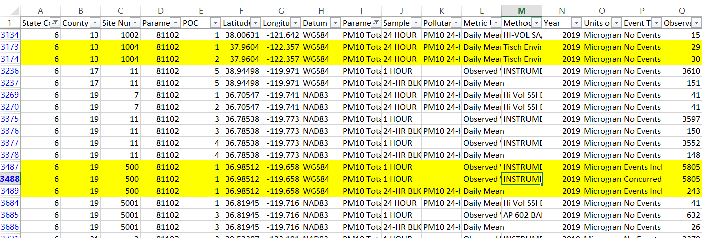
Figure 2: A selected screen capture showing part of the .csv data file from the EPA for the year 2019. The first yellow highlight shows a site with two FRM POC and no extreme events. The lower yellow highlight shows a site with a single FEM sensor that has extreme events and has, in the third highlighted row, been smoothed from hourly averages to daily averages. Columns A-C defines a unique site, Column E shows the POC, Column J the sample averaging period, Column P whether extreme events are included

Data Columns

Each of the EPA’s annual summary files is a .csv with 55 columns, as described in table 4. The data columns include the Arithmetic Mean as well as the 99^th, 98^th, 95^th, 90^th, 75^th, 50^th, and 10^th Percentiles of all the observations made at that site by that instrument and for that pollutant. For this report, the arithmetic mean was used as the statistic.

In addition to the main data file, a .csv file containing metadata for each site was used. Its columns are outlined in table 5.

Site Identification	Pollutant Metadata	Observation Metadata	Data	Other Metadata
State Number	Parameter Name	Year	Arithmetic Mean	Local Site Name
County Number	Sample Duration	Units	Arithmetic Standard Deviation	Address
Site Number	Pollutant Standard	Event Type	1st Max Value	State Name
Parameter Code	Metric Used	Observation Count	1st Max Date Time	City Name
POC	Method Name	Observation Percent	…	CBSA Name
Latitude		Completeness Indicator	…	Date of Last Change
Longitude		Valid Day Count	4th Max Value
Datum		Required Day Count	4ts Max Date Time
		Exceptional Data Count	1st Max Non Overlapping Value
		Null Data Count	1st Max Non Overlapping Date Time
		Primary Exceedance Count	99th Percentile
		Secondary Exceedance Count	98th Percentile
		Certification Indicator	95th Percentile
		Number of Observations below MDL	90th Percentile
			75th Percentile
			50th Percentile
			10th Percentile

Table 4: Names of all the column headers in a raw data file containing annual air pollution data from the EPA. Column headers are organized by general category and then listed in order of appearance. So State Number is the 1^st column, County Number is the 2^nd and Parameter Name is the 9^th. The exact definitions of each column can be found at the EPA website: https://aqs.epa.gov/aqsweb/airdata/FileFormats.html#_content_3

State Code	Latitude	First Year of Data	Networks
County Code	Longitude	Last Sample Date	Reporting Agency
Site Number	Datum	Monitor Type	PQAO
Parameter Code			Collecting Agency
Parameter Name			Exclusions
POC			Monitoring Objective
			Last Method Code
Local Site Name			Last Method
Address			NAAQS Primary Monitor
State Name			QA Primary Monitor
County Name
City Name
CBSA Name
Tribe Name		Extraction Date

Table 5: Names of column headers in metadata file describing the particulars of each site. Full details on the EPA website https://aqs.epa.gov/aqsweb/airdata/FileFormats.html#_format_2

4.10 Data Description

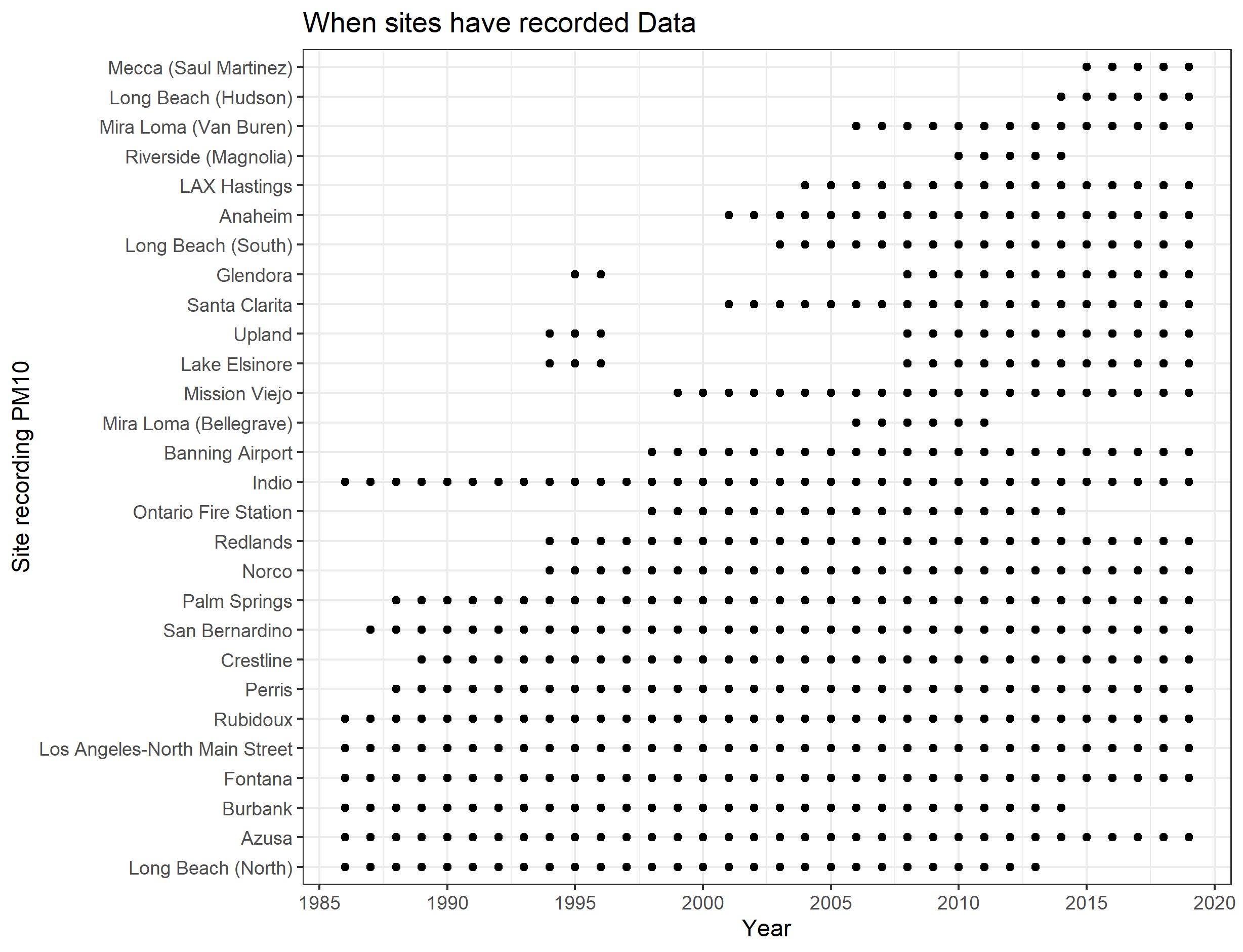
Figure 3: This figure shows how the network developed over time. We can see that sites are generally added to the network, that 5 sites have been removed, and that 5 sites started in 1986. A handful of sites has the unusual behavior of being taken offline and then removed. These are sites that only had FRM monitoring, no FEM.

Figure 4: Each box shows the general pattern of mean PM₁₀ observed each year. The red line shows how the number of active sites recording in the network (and therefore the number of observations feeding into each box) increases to the present day.

From 1986 to 2019 there are 28 unique sites monitoring $PM_{10}$ within the SOCAB. Figure 3 shows when sites are included in the network and when they are removed. Three sites (Glendora, Upland and Lake Elsinore) stop being recorded in 1997 and then restart in 2008. Why this happens, is unclear, but it only occurs in sites with only continuous FEM monitoring (as opposed to scheduled FEM sampling). The timeline coincides with regulatory changes to standards, but we have been unable to learn the reason for the sites’ discontinuation and restart.

Figure 4 summarizes the yearly mean $PM_{10}$ and shows how, over time, the number of sites has increased while the overall concentration in the area has gone down. The trend in $PM_{10}$ will be examined later.

Network Trends

Here are several plots showing traces of each site compared to the rest of the network. If the network is being biased consistently over time towards a certain goal, we would expect to see some difference between sites kept in the network vs those removed from it.

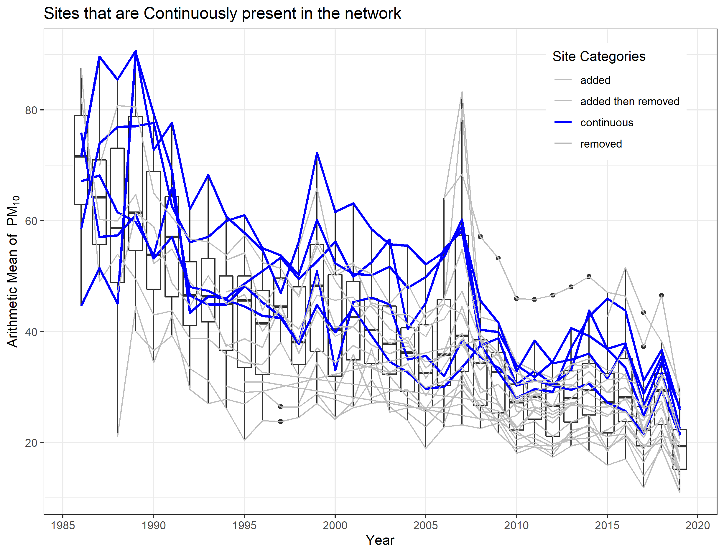
Figure 5: This figure highlights the traces of all the sites that started in the network and have not been removed. We can see that in later years the lower part of the boxes is not covered by these traces, indicating some possibility of preferential sampling. In the case when a site had multiple POC in a year, the value at the trace is the mean of all POC at that site for that year.

Figure 5 shows the sites that are active from 1986 to the present day, labelled as continuously present. The continuously present sites tend to be above the mean in more recent years. If sites maintain their relative position in the overall distribution, this suggests the early years are biased towards higher sites.

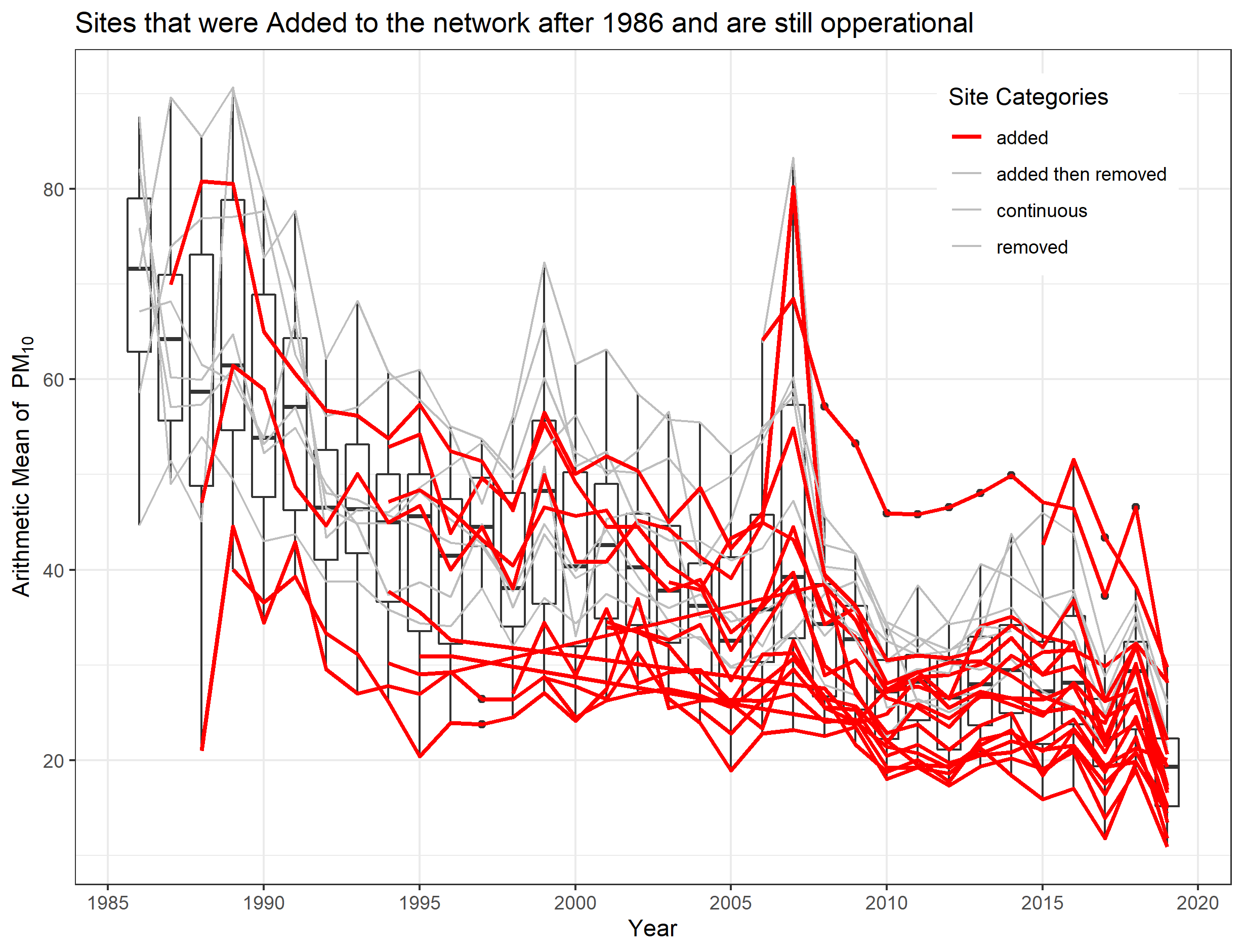
Figure 6: Here are highlights of all the sites that were added after 1986. It appears that there are more traces in the lower portion of the boxes, which is the required complement of the pattern shown in the previous figure. Again, in the case when a site had multiple POC in a year, the value at the trace is the mean of all POC at that site for that year.

Figure 6 shows how sites added to the network tend to fill out the bottom half of the distribution in later years. This is the inverse of the idea demonstrated in the previous figure (Figure 5).

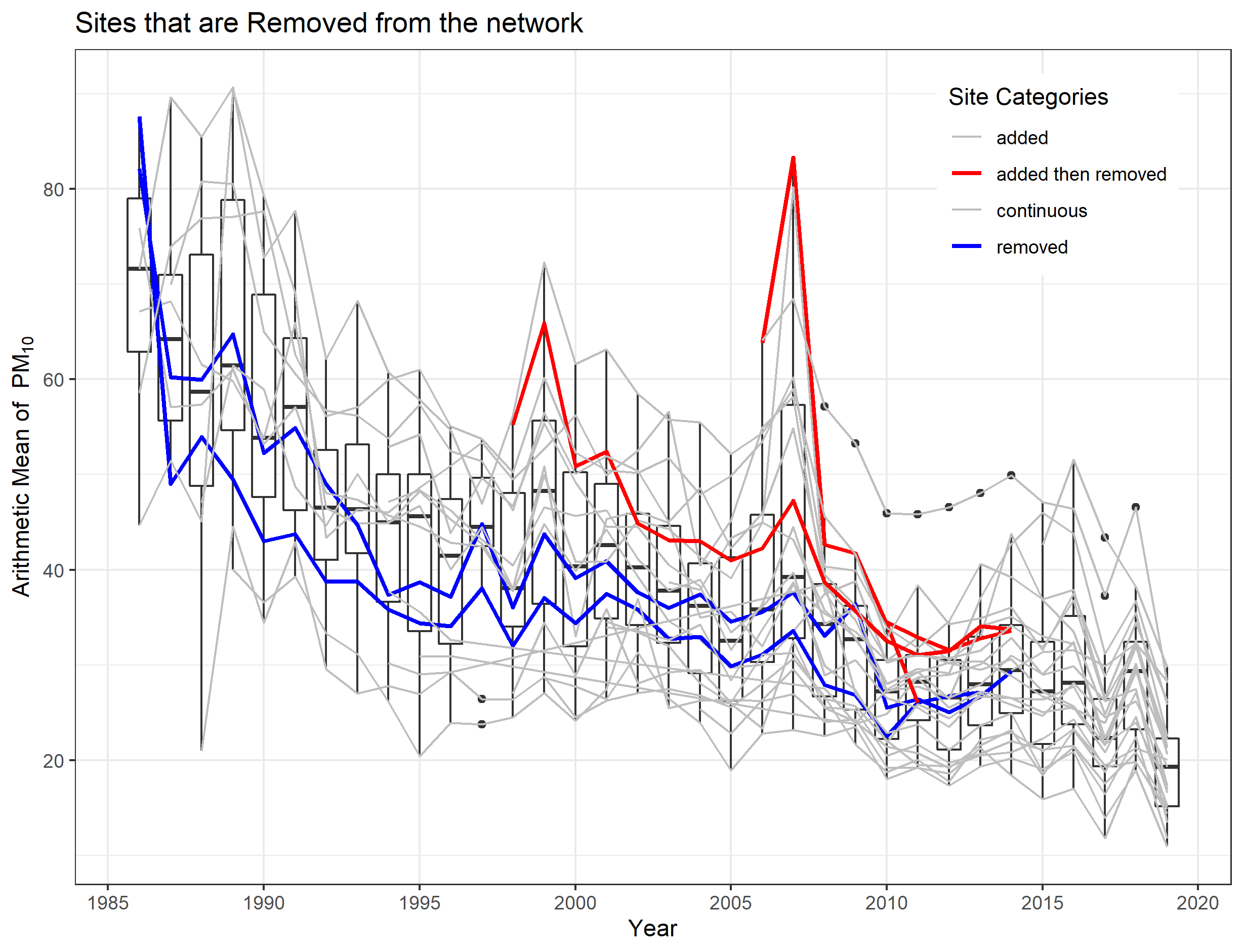
Figure 7: This figure highlights the sites that were dropped from the network. In Blue are two sites that started in 1986 but were then removed. In Red are three sites that were added to the network after 1986 and have been since removed.

Figure 7 highlights the five sites that were dropped from the network. Two of them were part of the original network in 1986, and tend to fall below the yearly mean. The other three were added to the network and tend to be above the yearly mean. This behavior is opposite to that seen in the plots of continuous sites and site that were added and kept. The sites that start in the network in 1986 and remain throughout tend to be above the mean, but the two that were removed are below the mean. The sites that were added to the network tend (to a lesser degree) to be below the mean, but those that were added and then removed tend to be above it.

Site Location

Figure 8 shows the location of sites in the SOCAB. Note that they are not all present simultaneously. It appears that some sites replace others. For example, Long Beach (North) and Long Beach (Hudson) are very close to each other and one stops while the other starts the next year. This lack of Independence in site selection was ignored.

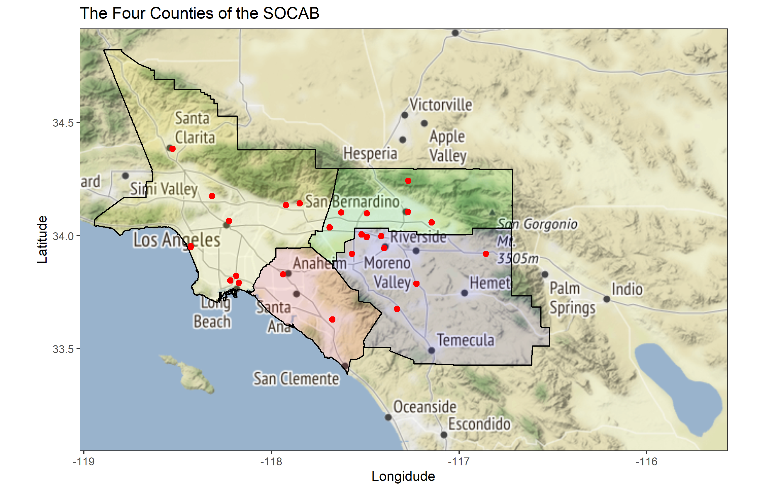
Figure 8: This map shows the SOCAB in relation to the Los Angeles region. It includes 4 counties, Orange County (Pink), Los Angeles County (Yellow), Riverside County (Blue), and San Bernardino County (Green). Only Orange County is entirely part of the SOCAB and the other counties extend into other air basins. Monitoring sites that are included in this study are red dots.

Site Metadata

The EPA and SCAQMD record additional descriptive information about each site. This includes:

• Land Use: Figure 14 shows the Land Use, describing whether the site is residential, commercial, industrial, or agricultural. Most (17) sites are residential, 3 sites are Industrial, 6 sites are Commercial, 1 is Agricultural, and Indio (a site that starts in 1986 and never dropped) has no stated land use.

• Location Setting: Figure 15 shows the Location Setting, describing whether the site is Urban (7 sites), Suburban (19 sites), or Rural (2 sites). Interestingly, the rural and suburban bracket the urban making a sandwich.

• Monitoring Objective: Figure 16 shows the Monitoring Objective, describing what the site is recording. Options include Extreme Downwind, Highest Concentration, Other, Population Exposure, Unknown, and Upwind Background.

Monitoring Purposes

Every site has at least one monitoring purpose. Some sites have mismatched site categories between the two 5 year reports. But we have not been able to determine if these are typos (other, more clear-cut typos have been found in the report) or if different monitors at the same location have a different category for some reason. Here are the sites that mismatch:

• San Bernardino (#060719004) is categorized as High Concentration except for the 2010 continuous monitor which is Population Exposure

• LAX Hastings (#060375005) is categorized as Population exposure and Population Exposure / Background in 2015

• Palm Springs (#060655001) is categorized as High Concentration except for 2010s FEM monitor which is Population Exposure.

The site category was only High Concentration and Population Exposure categories (LAX Hastings being the one exception, being both PE and HC in 2015 for the FEM sensors)

2010 (Monitoring Purpose)		2015 (Monitoring Purpose)
Long Description	Two-Letter Code	Long Description	Two-Letter Code
High Concentration	HC	Highest Concentration	HC
Representative Concentration	RC	Population Exposure	PE
Impact	IM	Source Orientated (impact)	IM
Background	BK	General Background	BK

Table 6: Comparison of Terminology describing the category each site is placed into for the 5-year summaries. Seen in table 2 of the two summaries.

2010 (Monitoring Purpose)		2015 (Monitoring Purpose)
Long Description	Two-Letter Code	Long Description	Two-Letter Code
Background Level	BK		BK
High Concentration	HC		HC
Pollutant Transport	TP		TP
Pollutant Exposure	EX		EX
Source Impact	SO		SO
Representative Concentration	RC		RC
Special Purpose Monitoring	SPM	–	–
Trend Analysis	TR		TR
Site Comparison	CP		CP
–	–	Real-time Monitoring and Reporting	RM
–	–	Collocated	CO

Table 7: Comparison of terminology describing the purpose of each site, as described in table 3 of the 2010 and 2015 5-year summaries. Not all categories exist in both years, when one isn’t present a–is placed in the year for which it is absent.

POC

As discussed in Section 4.9 each site has at least one sensor, but many have more than one. These could be an FEM and a FRM monitor, instrument changes, or collocation for trials or calibration. This redundancy provides an interesting way to estimate the nugget effect, which is sensor uncertainty. Figure 9 shows traces for every POC at each site. An example of the instrument changes seems to happen in 1988 when all the sites that had been in operation before 1988 received at least one other POC that returned a consistently higher reading of $PM_{10}$ and the POC that was in operation before 1988 was discontinued. These sites are Azusa, Burbank, Fontana, Indio, Long Beach (North), Los Angeles-North, Palm Springs, Perris, Rubidoux, and San Bernardino.

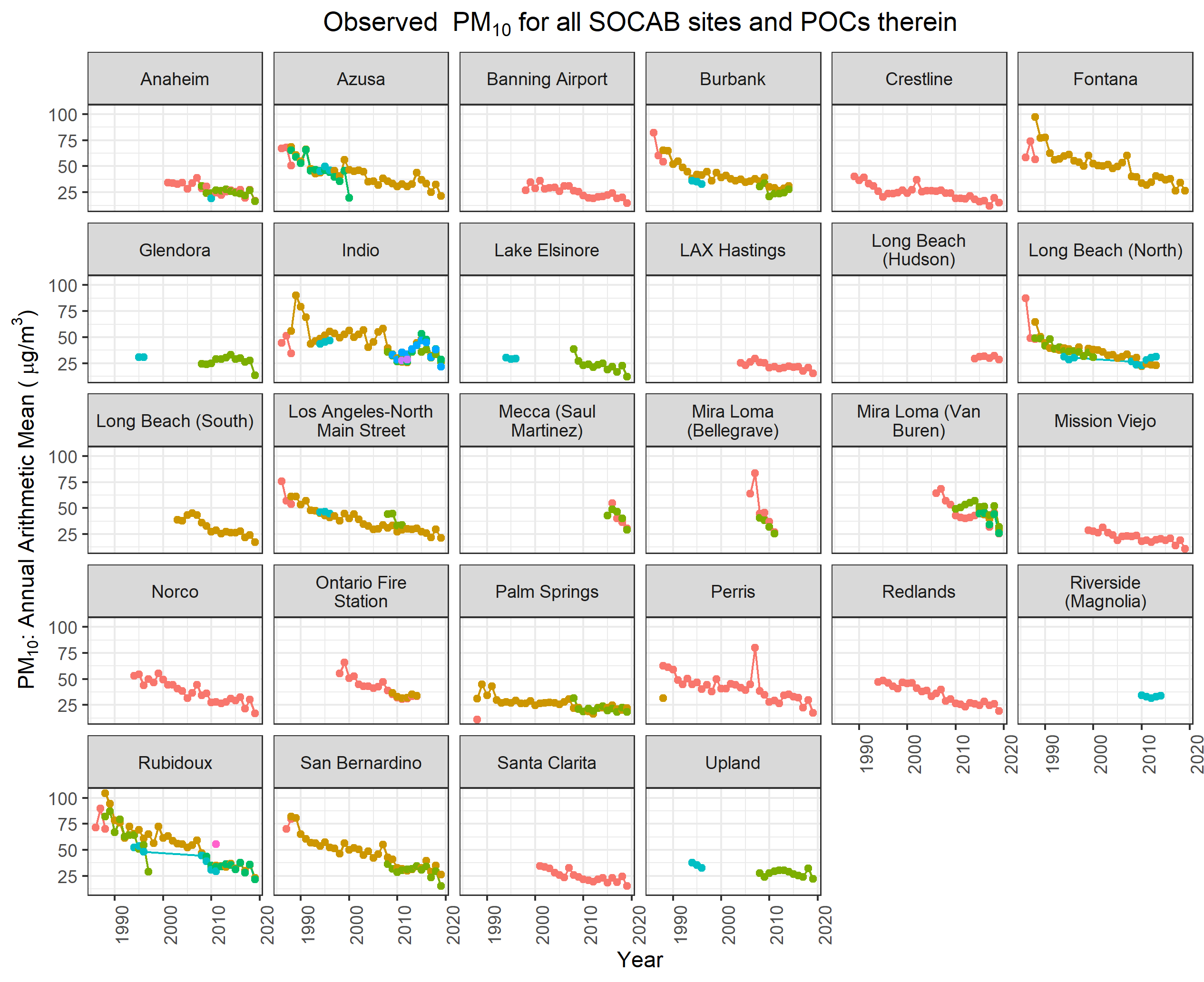
Figure 9: Traces showing every sensor (i.e. POC) recorded at each site. Colors are only to distinguish different POC and have no meaning between sites. Notice Azusa, Burbank, Fontana, Indio, Long Beach, Los Angeles-North, Palm Springs, Perris, Rubidoux, and San Bernardino all have a POC that stops being used in 1988 (generally colored red) and is replaced by another POC (generally brown) that consistently has a higher concentration of $PM_{10}$. Rubidoux and Long Beach (North) both have a POC (teal) that was discontinued in 1996 and then reestablished in 2007. These are continuous monitoring FEM along with Burbank, Glendora, Indio, Lake Elsinore, Los Angeles - North, and Upland which also have a teal sensor discontinued and eventually replaced by a green sensor.

4.11 Exploratory Data Analysis

Before applying complex INLA modelling to the question of preferential sampling, an exploratory data analysis was carried out. This analysis provided a sanity check for data acquisition and cleaning, highlight unusual patterns, and provide preliminary suggestions for preferential sampling.

Data Transformation

Ott (1990) suggests that particulate counts follow a log-normal distribution due to the physical processes that make the particulates. Taking the log of the raw counts helps to stabilize the variance. This was done by Cameletti et al. (2011) in their similar work examining $PM_{10}$ concentrations in Italy.

Since log scores are unitless, the raw $PM_{10}$ data were normalized to the mean $PM_{10}$ in 1986 and the log of that ratio was taken, as described in equation 12. In equation 12 $t$ is the year, $s$ is a unique site, $Z$ is the transformed data used for future calculations and modelling, and $PM10_{t,s}$ is the raw data for the year $t$ at site $s$. Finally, $PM10_{1986,\cdot}$ is the mean of the all observed $PM_{10}$ in 1986, 69.65397 $\mu g/m^{3}$. This log normalized value of the $PM_{10}$ is used for all future analyses.

$$Z_{t,s}=log(PM10_{t,s}/PM10_{1986,\cdot})$$ (12)

Temporal Effects

An initial examination of figure 4 shows the concentration of $PM_{10}$ decreasing over time, as expected from the known history of particulate matter. This could be modelled as either a fixed or a random effect. Both options were examined, and the results are described in this report. In this preliminary investigation, all spatial correlations were ignored.

After preliminary modelling, our focus is on describing preferential sampling, not the decrease in $PM_{10}$ overtime. Modelling the small perturbations with a Random Walk seemed likely to give a better understanding of what the sites are doing and so a better picture of any possible preferential sampling.

Fixed Temporal effects

The first way to model the temporal trend is with a linear model. While the general trend in means of figure 4 appears mostly 1st order to the eye, Shaddick and Zidek (2014) used a quadratic function to model the decreasing temporal trend in black smoke in the UK. That led us to investigate both first- and second-order models for the trend over time using equations 13a and 13b respectively:

$$Z_{t,\cdot} =\beta_{0}+\beta_{1}t+\epsilon$$ (13a)

$$Z_{t,\cdot} =\beta_{0}+\beta_{1}t+\beta_{2}t^{2}+\epsilon.$$ (13b)

Figures 10 and 11 show the results of first and second-order models being fitted to the log normalized $PM_{10}$ data. An Analysis of Variance (ANOVA) comparing the two models ($anova(model.lm.log,model.lm.log.quad)$) suggests a small but significant improvement of the second order model ($Pr(>F)=0.0492$) compared to the 1st order.

Both models do a good job of whitening the overall residual of the annual mean, as seen in the autocorrelation function (ACF) and Partial Autocorrelation Function (PACF) plots. This suggests there might not be an autocorrelation AR(1) process, unlike the model used by Cameletti et al. (2011).

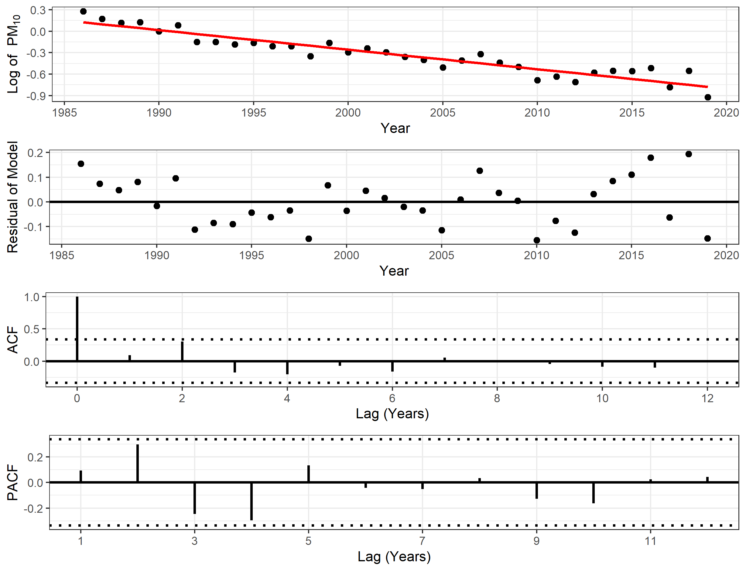
Figure 10: Results of a linear fit to a log transformation of the $PM_{10}$ data. The line is the model $Z_{t,s}\sim Year$, and has a slope of -0.027 and adjusted $R^{2}$ of 0.88. The ACF and PACF suggest that the process remaining is probably white noise. Dots are the Median of the arithmetic mean of each year. The dotted line shows a confidence limit of $qnorm((1+ci)/2)/sqrt(n)$, R’s default for ACF and PACF. This stems from Chatfield’s Analysis of Time Series (1980), in which he describes how the variance of the autocorrelation coefficient at lag k, is normally distributed at the limit, and that $Var(rk)\sim 1/N$ (where N is the number of observations).

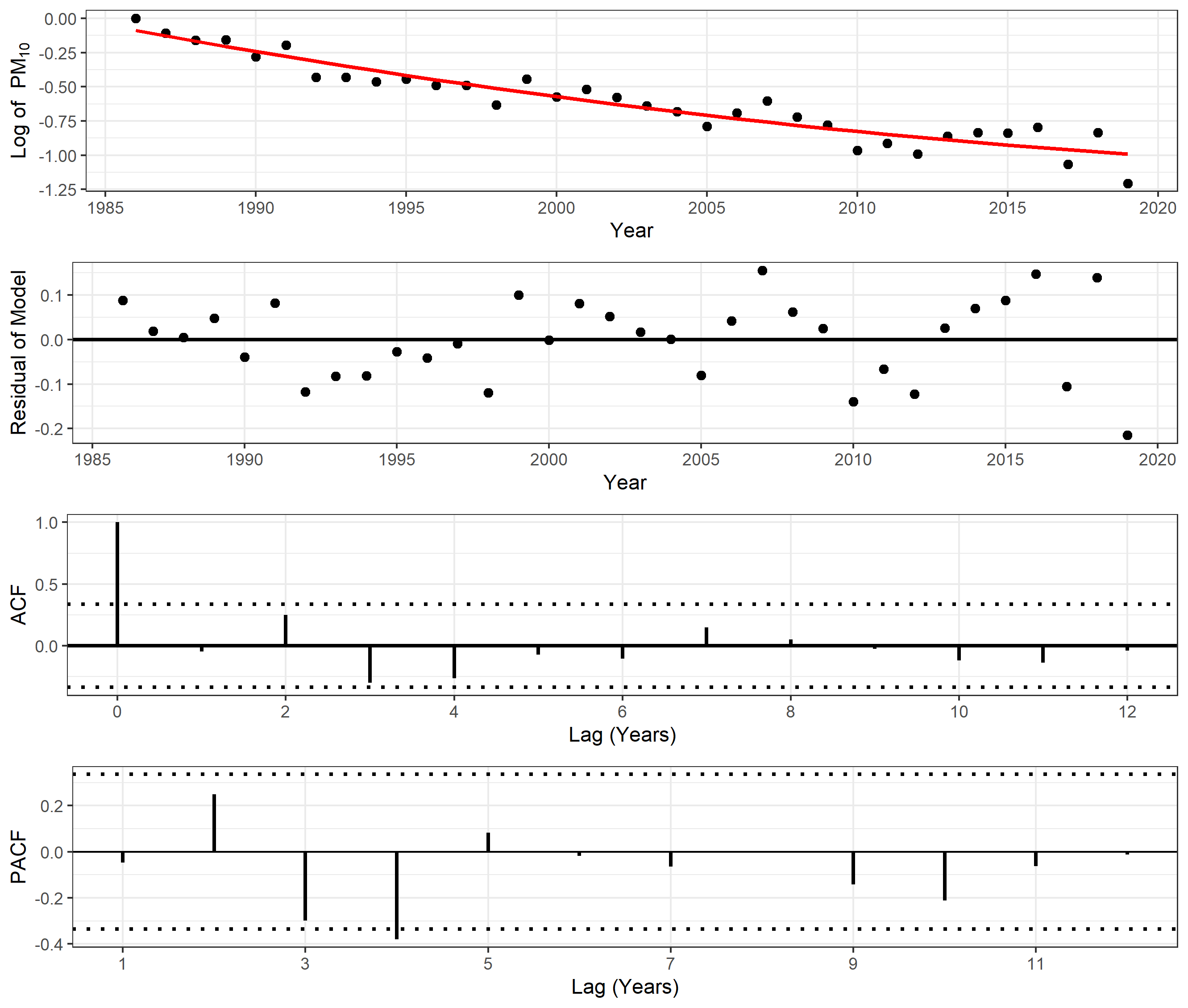
Figure 11: Results of a linear fit to the $PM_{10}$ data. The line is the model $Z_{t,s}\sim\beta_{1}Year+\beta_{2}Year^{2}$ and has coefficients $\beta_{1}=-1.56$ and $\beta_{2}=0.00038$ and adjusted $R^{2}$ of 0.90. The ACF and PACF plots of the residuals suggest there might be a MA(1) or AR(1) process. Dots are the Median of the arithmetic mean of each year. The dotted line shows a confidence limit of $qnorm((1+ci)/2)/sqrt(n)$, R’s default for plots of ACF and PACF.

Temporal Trend as a Random Walk

An alternative approach to accounting for a broad-scale trend in time is to use a random variable. The logic supporting the use of a random variable over a fixed effect lies in our lack of interest in estimating the annual decrease, and a model that can be more adaptive to yearly fluctuations can fit closer and give a better understanding of the field at the time. Two options are a random walk and a 1-dimensional Matérn interpolation with INLA. Because the random walk is simpler, that was chosen.

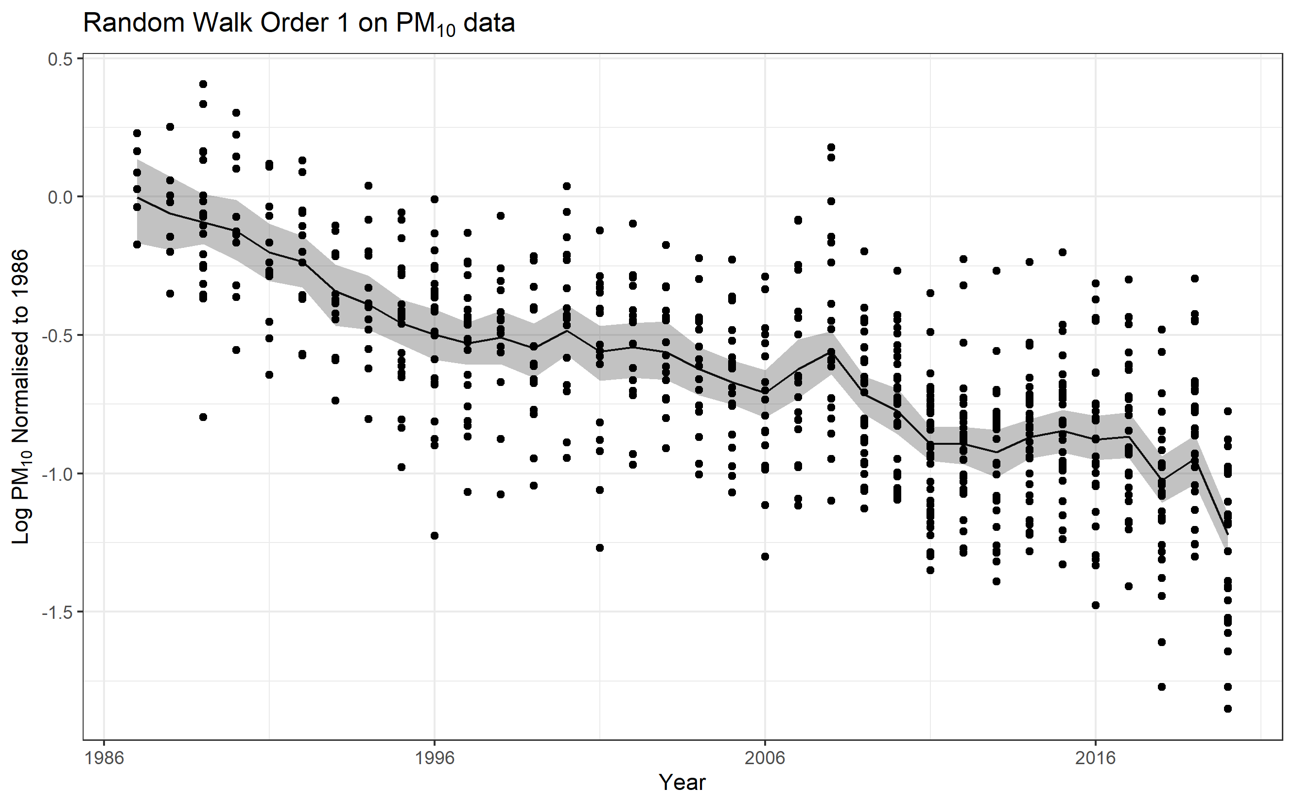
Figure 12: First order Random Walk smoothing sets a prior on the difference between each observed value $f(\kappa_{i})$. Like so: $f(\kappa_{i+1})-f(\kappa_{i})\tilde{}N(0,\tau)$

Figure 13: Second order Random Walk smoothing sets a prior on the difference between each observed value $f(\kappa_{i})$. Like so: $f(\kappa_{i+1})-2f(\kappa_{i})+f(\kappa_{i-1})\sim N(0,\tau)$

First-order smoothing, shown in Figure 12, looks spiky, and second-order smoothing, 13 seems better. Table 8 describes the results of the two orders of smoothing, and the DIC criterion suggests that the 1st order smoothing is marginally better than the 2nd order smoothing.

As discussed in the section on priors, section 4.4, the PC prior for the precision of the RW is set as the empirical SD of the data, which is $0.3729848$ when not accounting for the structure of sites and POCs.

⬇

1 pc_prior <-list(theta =list(prior =‘‘pc.prec’’,

2 param =c(data.emp.sd,0.01)))

Parameter	RW 1	2
Model WAIC	1.187e+02	1.285e+02
Model DIC	1.187e+02	1.283e+02
Intercept Mean	3.407793e-05	2.074067e-05
Intercept SD	31.62663	31.69167
RW trend range, mean:	[-1.2189, -0.00401586]	[-1.19403, 0.0299855]
RW trend sd, range:	[31.6266, 31.6267]	[31.6917, 31.6918]
Hyperpar: Precision of Gaussian observation Mean	14.9708	14.38641
Hyperpar: Precision of Gaussian observation SD	0.8224243	0.5420988
Hyperpar: Precision of Random Walk Parameter Mean	106.8693	814.72112
Hyperpar: Precision of Random Walk Parameter SD	41.5575799	961.1867062

Table 8: Comparison between exploratory models for a RW1 and RW2 model for the trend over years. Neither model has a spatial component, and they treat sites and POCs in the same year as IID instead of nesting them in any way: y = intercept + RW.

The R package inlabru to generate a Random walk of order one on the time series using the following code:

⬇

1cmp.spline1.PM10 <- log.Arthmt.M ~ Intercept + trend(map = yeari,

2 model = ‘‘rw1’’,

3 constr = FALSE,

4 n = n_year,

5 hyper = pc_prior)

6bru.spline1.PM10 <- bru(cmp.spline1.PM10,

7 family = ‘‘gaussian’’,

8 data = test)

Similarly, a second-order random walk in R was generated as follows:

⬇

1cmp.spline2.PM10 <- log.Arthmt.M ~ Intercept + trend(map = yeari,

2 model = ‘‘rw2’’,

3 constr = FALSE,

4 n = n_year,

5 hyper = pc_prior)

6bru.spline2.PM10 <- bru(cmp.spline2.PM10,

7 family = ‘‘gaussian’’,

8 data = test)

4.11.1 Metadata

Finally, gross patterns in the mean could exist and be described by the metadata available and included in a final model as fixed effects. Here is a brief discussion of the categorical metadata variables available from the SCAQMD and the EPA that were examined as possible inclusions.

The three variables, which were examined, were Land Use (e.g. commercial, residential, industrial, agricultural), Land Density (e.g. urban, rural, suburban), and Site Classification (e.g. background, high concentration, population exposure).

A quick examination of the Land Use and Land Density, (both from the EPA’s metadata) in Figures 14 and 15 respectively, show that these categories will have little help in making predictions.

The SCAQMD provides the Site Classification. These categories seem to have different means from each other, see Figure 16, but only in that sites designed to capture high concentration do so. Since the effort is to describe preferential sampling and not relations to covariates, this tautology seems unhelpful for modelling the $PM_{10}$ field. Future work that tries to model site inclusion or removal might find the Site Classification useful.

Figure 14: This shows the site traces colored by the type of human activity being carried out in the vicinity of each site as defined by the EPA. In the case of multiple POCs in at one site, the mean of those POCs is taken. One site was given no category and is in Grey. The vast majority of sites are either Commercial (red, 6 sites total) or Residential (blue, 17 sites total) and these two categories are mixed relatively homogeneously. Industrial (light green, 3 sites total) and Agricultural (Orange, 1 site) sites stand out as generally being elevated above the IQR for each year’s observations, but have a handful of total sites.

Figure 15: This shows the site traces colored by the density of buildings at each site as defined by the EPA. In the case of multiple POCs in at one site, the mean of those POCs is taken. The three categories of site - Rural (2 sites), Suburban (19 sites), and Urban (7 sites) - are distributed in a way that suggests deliberate choice. Each category seems to be evenly split to have sites above and below the mean. Urban sites are closely clustered around the overall mean, Suburban generally surround the Urban sites, and the two Rural sites are relatively extreme.

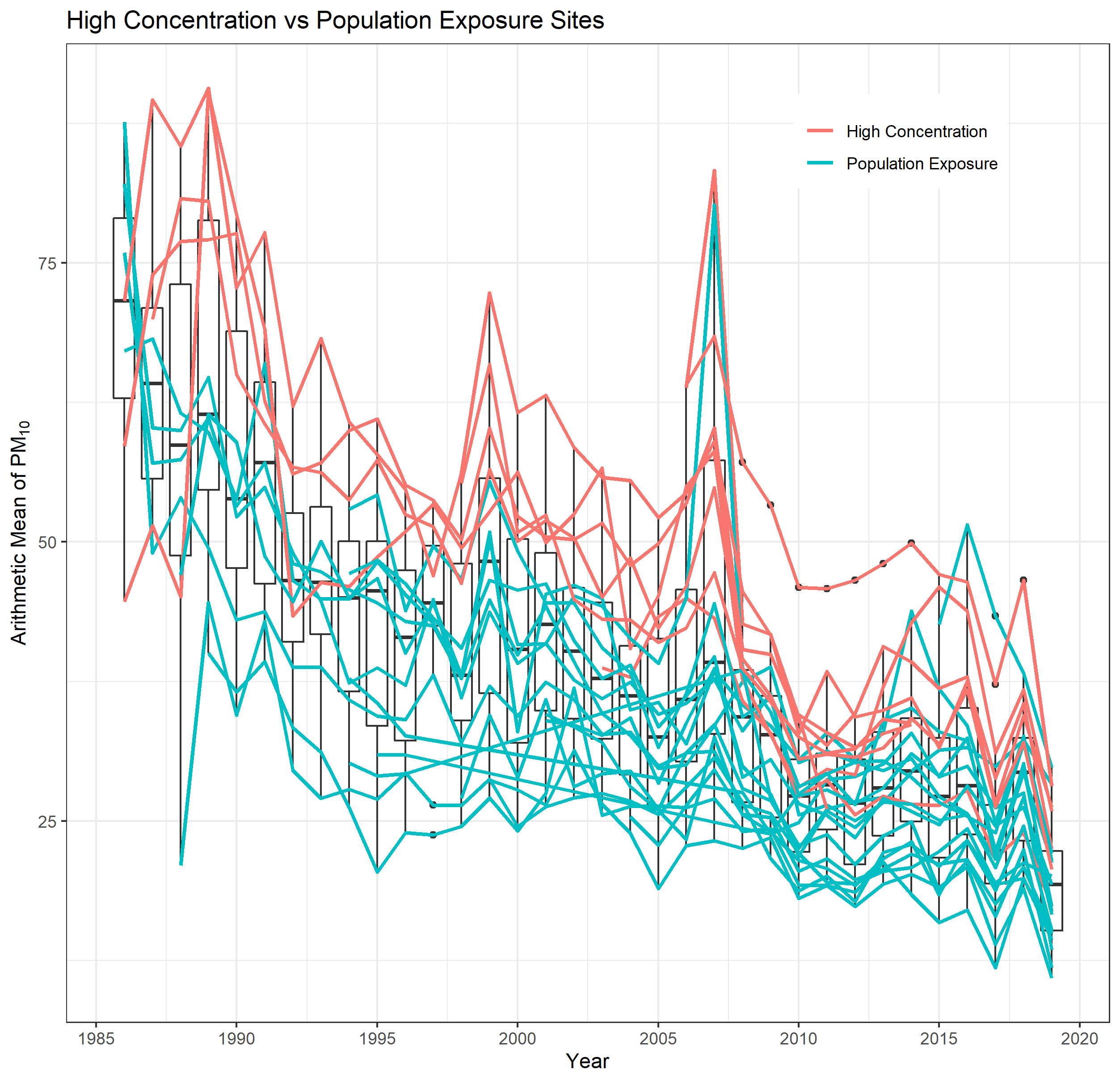
Figure 16: This shows the site traces colored by the Site Type category pulled from the SCAQMD 5-year reports. In the case of multiple POCs in at one site, the mean of those POCs is taken. On the rare occasion that a site had a different type in 2010 and 2015 or between FEM and FRM monitors, the most consistent type was used for that site. The sites designated High Concentration (9 total) are observing a higher concentration than the sites designated Population Exposure (19 total).

4.12 Traditional Spatial Modeling

Initial spatial modelling using Kriging with a Matérn covariance function examined each year’s variogram independently of other years. These produced inconsistent results. Each year’s fitted covariance had different parameters. Some possible reasons for this are:

• An insufficient number of sites in a single year leads to instability or non-identifiability in the model. We think this could be contributing to poor models in the early years.

• The sites are too far apart to resolve most of the curve of the covariance function. Since Cameletti et al. (2011) found a range of 275 km for $PM_{10}$ this seems unlikely to be a issue at the scale of the SOCAB.

• Biased sampling makes the estimate of the empirical variogram unreliable, with the bias in the semivariance’s estimate increasing with $u$ (Diggle and Ribeiro, 2007). If, as suspected, there is preferential sampling in the SOCAB this could be another reason that the semivariograms did not work well.

Variogram plots for each year and their parameter values are not included for brevity, but here are three examples demonstrating the range of success in modelling the variograms: Figure 17, Figure 19, and Figure 18. Figure 17 does not have enough sites to make a clear variogram. Figure 19 has plenty of sites, but exhibits a strange behavior with raised semivariance at short range that tails off at longer range. Finally, Figure 18 exhibits a nice behavior with a rise in semivariance over the closer distances and then a rough flattening as the range increases.

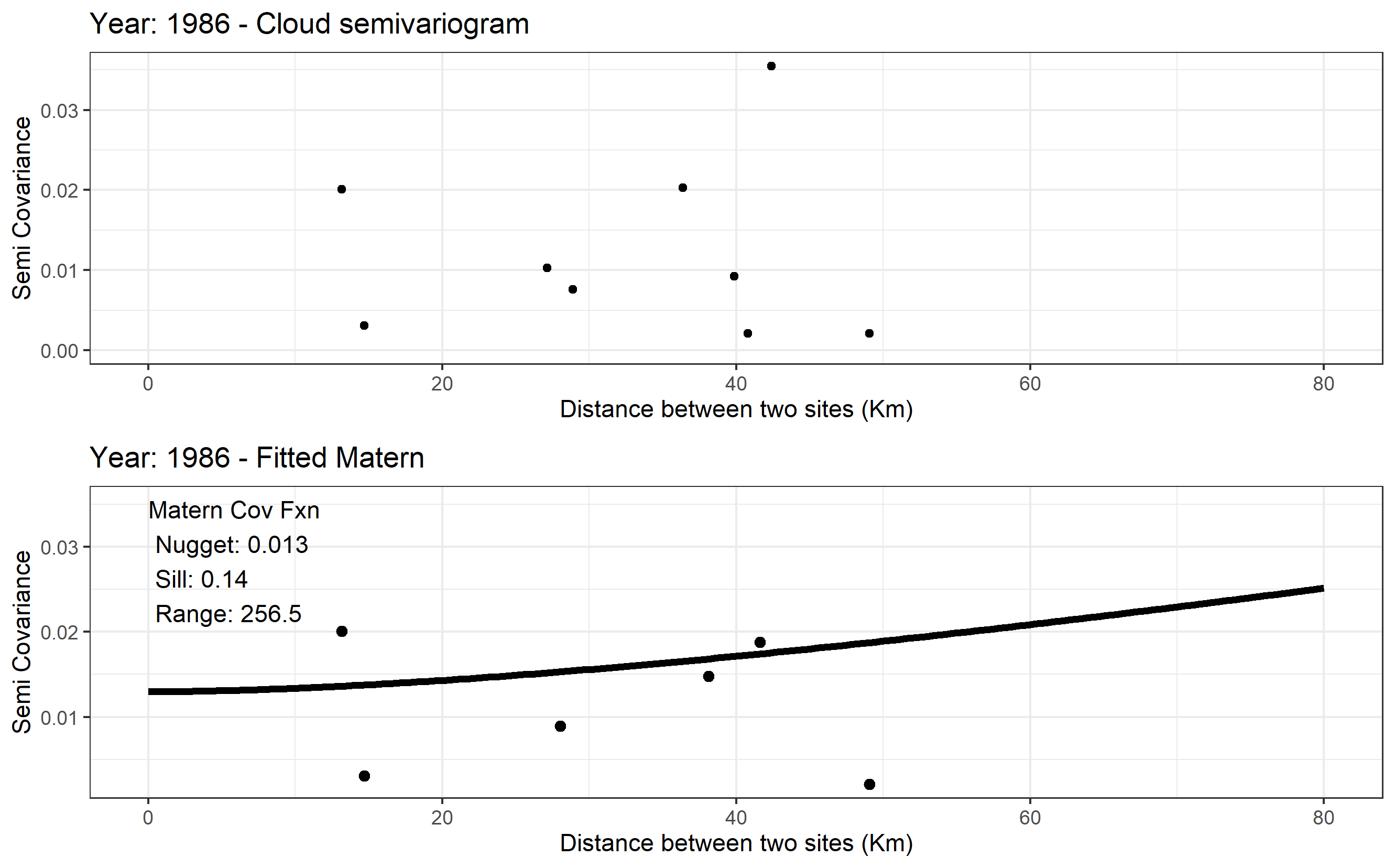
Figure 17: At the start of the network, a lack of sites poses a challenge to obtain a sufficient resolution to resolve a fitted variogram.

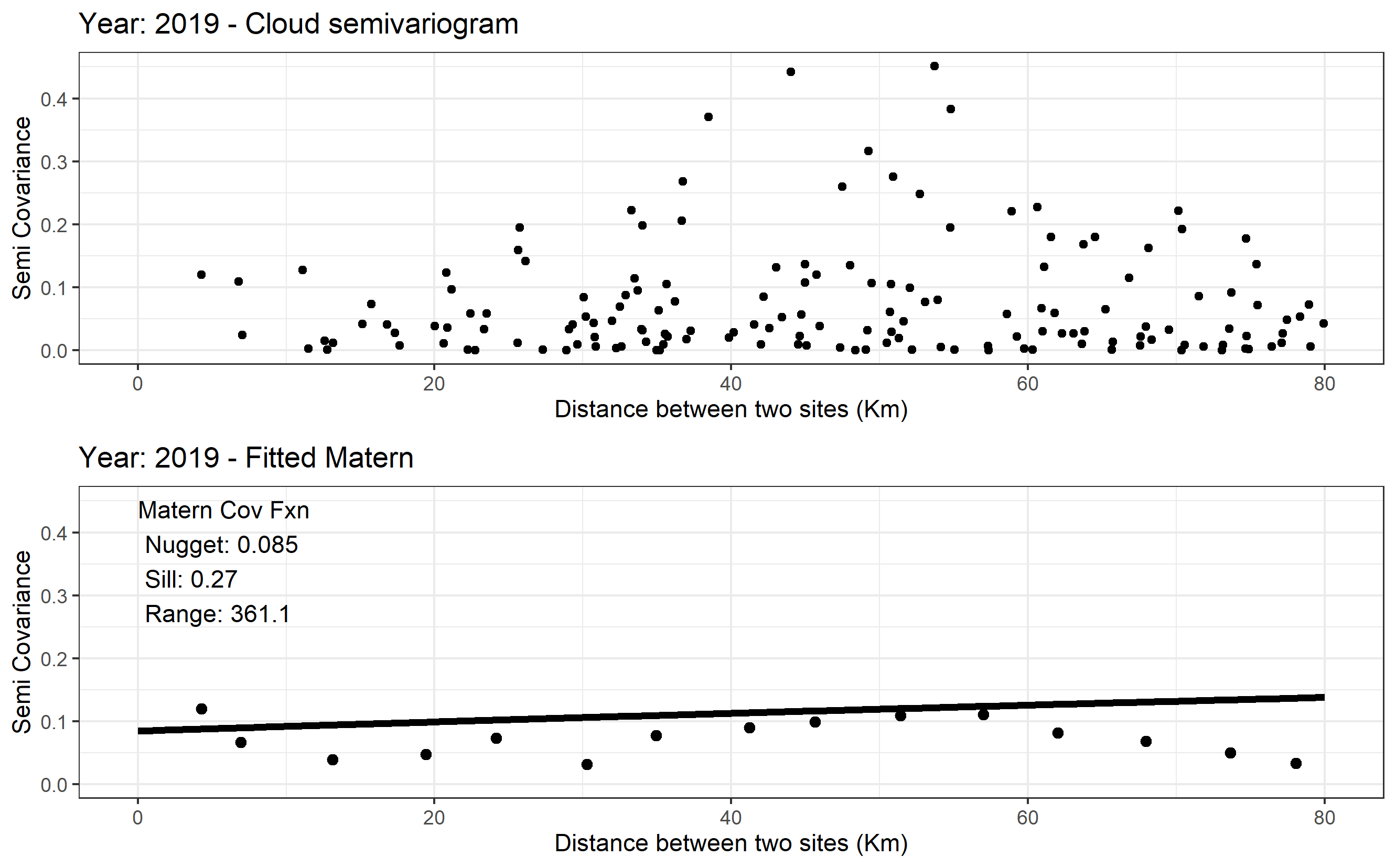
Figure 18: Even in later years, there was no guarantee of a good fit. Here the variogram has no clear trend early on, preventing the curve from being established.

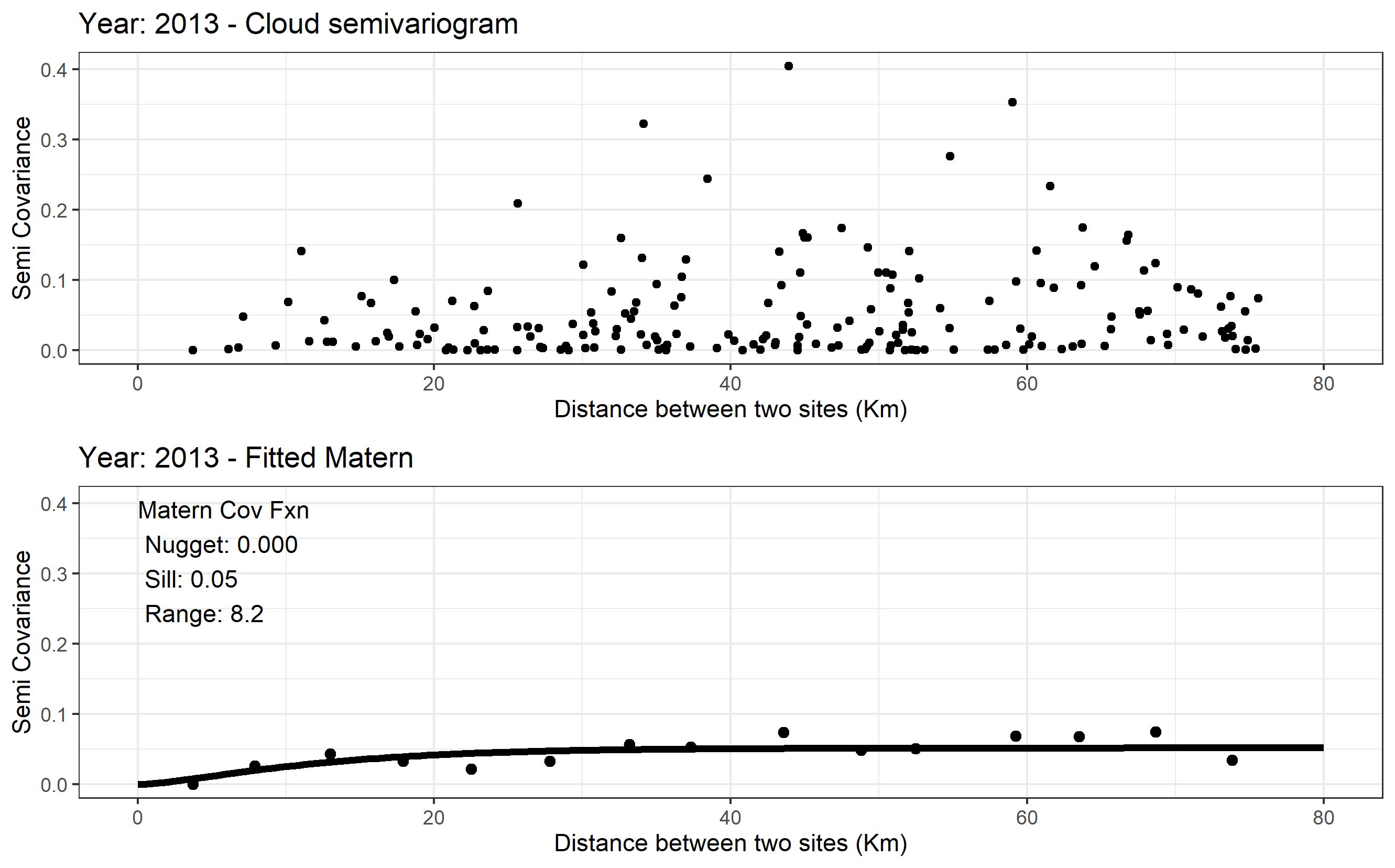
Figure 19: Here is one of the better-fitting years. Key to the success of these types is the small distance estimates having a lower semivariance than most of the rest of the sites.

5 Modeling with INLA

5.1 Mesh Construction

As discussed in Section 4.3, the mesh’s design is important for the subsequent modelling. Preliminary models using coarser meshes suggested the Gaussian Random Field (GRF) has a range of about 100 km. With that information and following Righetto et al. (2020), a maximum edge length of 20 km and a cutoff point of 5 km were chosen for the final mesh. The external maximum edge length was set at 40 km and the width of the offset kept 2-3 edge lengths between the inner boundary and the outer boundary. The final mesh can be seen in Figure 20 and was created using the code below.

⬇

1mesh1 <- inla.mesh.2d(loc = PM10.INLA.data.aea.SOCAB@coords,

2 boundary = SOCAB_union_sp,

3 offset = c(1,40),

4 max.edge = c(20, 40),

5 min.angle = c(21, 21),max.n=c(48000, 16000),

6 max.n.strict=c(128000, 128000),

7 cutoff=5

8 )

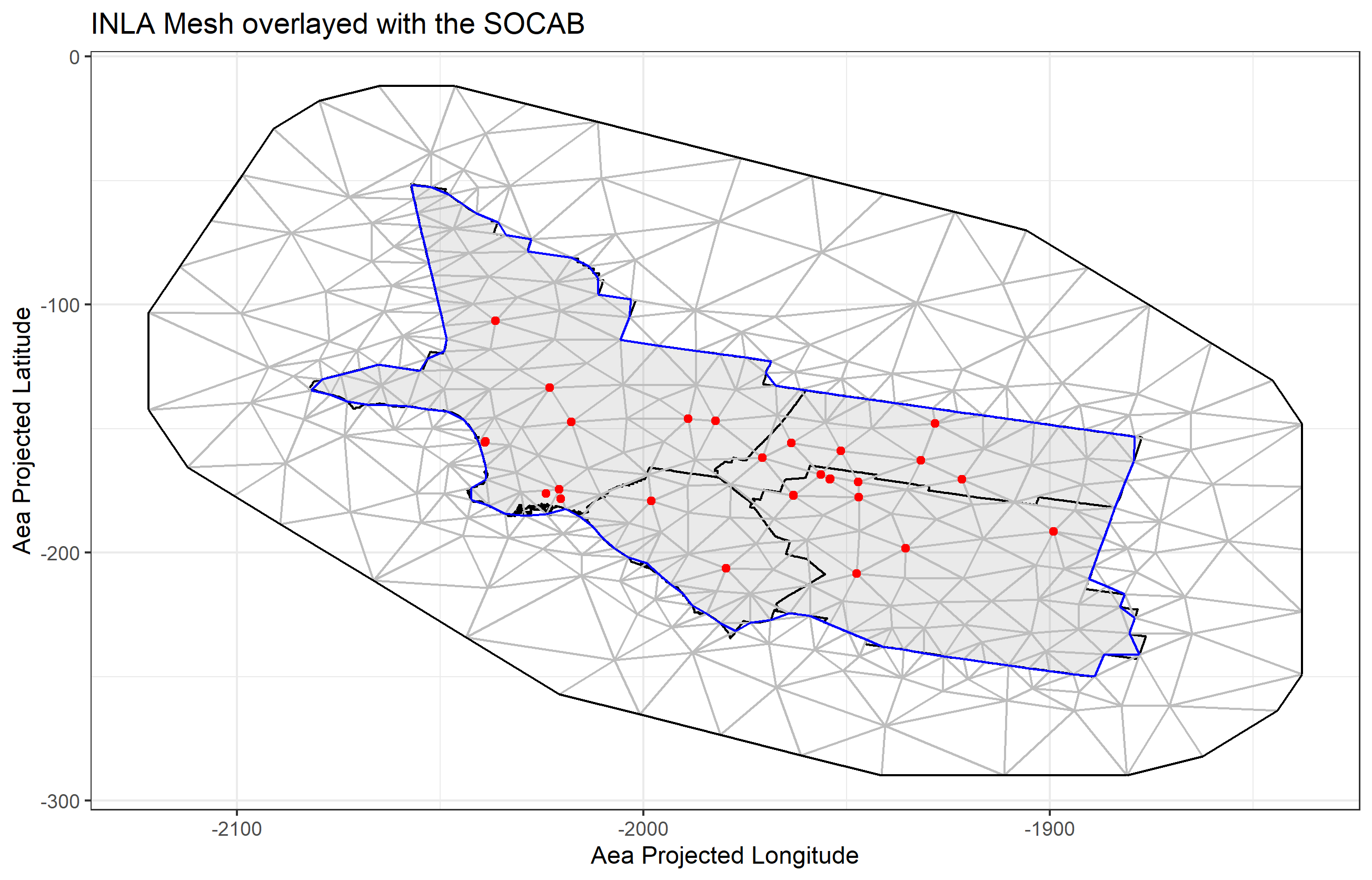
Figure 20: The mesh used for modelling, shown projected in the Albers projection. The red dots are the location of sites contributing data to the model. The blue line is the boundary of the SOCAB as defined in INLA. Under the blue line is a black line showing the actual legislated boundary. There are a few sites close to the interior boundary, but no sites near the outer boundary. By using sites as seed locations for the nodes, the problem of having multiple sites in one triangle was avoided.

5.2 Matérn Parameters

The Matérn covariance function has several parameters that must be either estimated or fixed. These are the smoothness, $\kappa$, and the PC priors for the Range and Variance, as discussed in Section 4.2 and Section 4.4.

Smoothness, $\kappa$

As discussed earlier in Section 4.2 the Matérn’s smoothness, $\kappa$, is fixed to make the choice of other parameters clear. Cameletti et al. (2011) used $\kappa=1$ for their Matérn function, we chose to use 1 as well.

Priors

Here are described the choices of PC priors for the range, variance, and random walk used to generate the covariance function.

5.2.1 Range

The PC prior for the range is based upon the smallest value that is reasonably expected for the range. This is done with the formula 14. The documentation for the PC prior suggests setting $p_{r}$ at 1%. Table 9 shows the range quantiles from the empirical variograms for each year, providing a guide for what value of $r$ to choose for the PC prior, we used $P(r<6)=0.01$.

$$P(r<r_{0})=p_{r}.$$ (14)

Quantile	Range (km)	Partial Sill
0%	4.34	0.00
1%	4.68	0.00
5%	6.17	0.00
10%	8.42	0.00
15%	9.37	0.012
25%	10.61	0.042
50%	20.55	0.066
75%	36.69	0.14
90%	349.42	1.65
95%	852.55	3.82
99%	2247.57	32.80
100%	2882.08	46.62

Table 9: Empirical Quantiles of the range and partial sill of the 34 yearly Variograms using 1986 normalized log $PM_{10}$.

Cameletti et al. (2011) Found range of 275 km and 1046 km for PM10 in Piedmont valley

The EPA describes spatial scale as follows:

“Thus, the spatial scale of representativeness is described in terms of the physical dimensions of the air parcel nearest to a monitoring site throughout which actual pollutant concentrations are reasonably similar.”

In CFR40-58, the $PM_{10}$ sensors are defined as having a neighborhood scale up to 4 km. This implies that it would be physically impossible to resolve a range that is about 4 km or smaller. With the information about the spatial scale of the sites from CFR40-58 and the combination of the empirical variograms of the SOCAB and known range of $PM_{10}$ from previous studies, it is reasonable to have $P(\rho<3)=0.01$. Implying it is unlikely that the range is smaller than 3 km.

Variance

The PC prior takes user input on the upper tail quantile and the probability of exceeding it as equation 15. Using the 34 years of empirical variograms, we get the quantiles shown in 9 for the partial sill, and then used $P(\sigma>35)=0.01$ as the prior on the partial sill.

$$P(\sigma>\sigma_{0})=p_{\sigma}$$ (15)

5.2.2 Random Walk

The RW used in the full model was initiated with the same priors as the RW performed during the data exploration, see Section 4.11.

5.3 Choice of Covariance Structure

The final model was chosen from a range of options by comparing the DIC of models with different structures. These structures were expanded from the core model of a single Matérn GRF through the addition of an RW over time, an AR(1) process over time, and combinations of these. Cameletti et al. (2011) used a Matérn field with an AR(1) process to account for shifts between observations periods. This modelling was done with the full dataset.

Table 10 summarizes the model results for these different covariance structures. The models with smaller DIC are more attractive options for further modelling. The model chosen is number 4, the combined GRF and AR(1) process, which is the same structure as that used by Cameletti et al. (2011).

Model Cov Structure	DIC
Matérn	2.385e+02
Matérn and RW1	-8.385e+02
Matérn and RW2	-8.349e+02
Matérn, RW1, and AR1	-9.173e+02
Matérn, RW2, and AR1	-8.969e+02

Table 10: The data used is the log of the normalized data as shown in equation 12. The covariance structures are listed in order of increasing complexity. RW(1) is the smoothing that describes the transition of the overall mean from one year to the next. GRF is the Matérn function taken as an overall mean for the whole year.

The equation describing the final model is as follows:

$$Z(s,t)=\beta_{0}+\Delta y_{t}+y(s,t)+\epsilon(s,t)$$ (16a)

$$\Delta y_{t}=y_{t}-y_{t-1}$$ (16b)

$$y(s,1) \sim N\left(0,\frac{\sigma^{2}_{w}}{(1-a^{2})}\right) ,|a|<1$$ (16c)

$$y(s,t) =ay(s,t-1)+w(s,t) ,t>1$$ (16d)

$$cov(w(s,t),w(s,t^{\prime}))=\begin{cases}0\text{ if }t\neq t^{\prime}\ ,\\ \sigma^{2}_{w}\gamma(u)\text{ otherwise, }\gamma(u)\sim\text{Mat\'{e}rn.}\end{cases}$$ (16e)

Final Model

Table 11 gives the results of the final model, performed on a randomly selected 90% of the data, holding the other 10% for validation, see Section 5.4 for details. The model has a RW1 structure portraying the trend over time, a Matérn covariance function describing the spatial structure and an AR(1) function describing how that structure changes over time.

	Value	SD
WAIC	-7.958e+02
DIC	-8.022e+02
Intercept	-0.0005082417	31.58598
RW1	[-1.36122, -0.114299]	[31.5861, 31.5861]
Matérn	[-0.408501, 0.58749]	[0.0812534, 0.349748]
Hyperpar Gaussian Prec.	73.6006189	2.811640470
Hyperpar RW1 Prec	60.1411588	7.967774153
Hyperpar Matérn Range	23.8506006	6.017936799
Hyperpar Matérn Stdv	0.2729190	0.023497256
AR(1) rho	0.9923009	0.001750823

Table 11: Summary results of model that has RW1 over the years, a Matérn spatial process and an AR(1) term. The RW1 and Matérn are random variables and so take on a unique value at each site.

The following code is how the model was constructed in R with INLABru.

⬇

1cmp.Matern.RW1.AR1.PM10.subsample = log.Arthmt.M ~

2 Intercept + trend(map = year, model = ‘‘rw1’’,

3 constr = FALSE, n = n_year, hyper = rw_pc_prior) +

4 myspde(map = coordinates, group = year,\ngroup = n.year,

5 model = inla.spde2.pcMatern(mesh1, alpha = Matern_alpha,

6 prior.range = Matern_pc_prior_range,prior.sigma =

7 Matern_pc_prior_sigma),mesh = mesh1,control.group=list(model=‘‘ar1’’))

8bru.Matern.RW1.AR1.PM10.subsample = bru(cmp.Matern.RW1.AR1.PM10.subsample,

9 family = ‘‘gaussian’’, data= PM10.INLA.data.aea.subsample.SOCAB)

5.4 Prediction and Validation

The $PM_{10}$ surface for each discrete year was interpolated using the model described in Section 5.3. This surface was used for subsequent preferential sampling testing as well as model validation. The prediction was performed on a grid of pixels covering the SOCAB with each pixel approximately 2 km square as defined by the Lambert projection. After predicting the surface, the results were used to examine whether the model did a “good job” of describing the known observations.

Withholding 10% of Data

. Model validation was done while holding out a randomly selected 10% of the data. The sites and years that were withheld can be seen in Figure 21. The model was then used to predict that 10% and the results compared to the actual values. The difference between the prediction and the actual observed value can be seen in Figures 22 and 23. This is a basic but easy-to-implement method that is not computationally intensive.

It is concerning that Figure 22 shows such a high percentage of sites whose prediction interval does not contain the actual observed value. Theoretically, only 5% of the validations should not contain the actual value within the 95% prediction interval. The variance could be underestimated, or the model could be too smooth.

Figure 23 suggests that there isn’t any obvious prediction problem at individual sites, so maybe it is the variance that is too small.

Figure 21: The red dots are observations that were kept out of the model for use in future validation. Eighty (ten percent) of the 822 total observations were held back, chosen at random

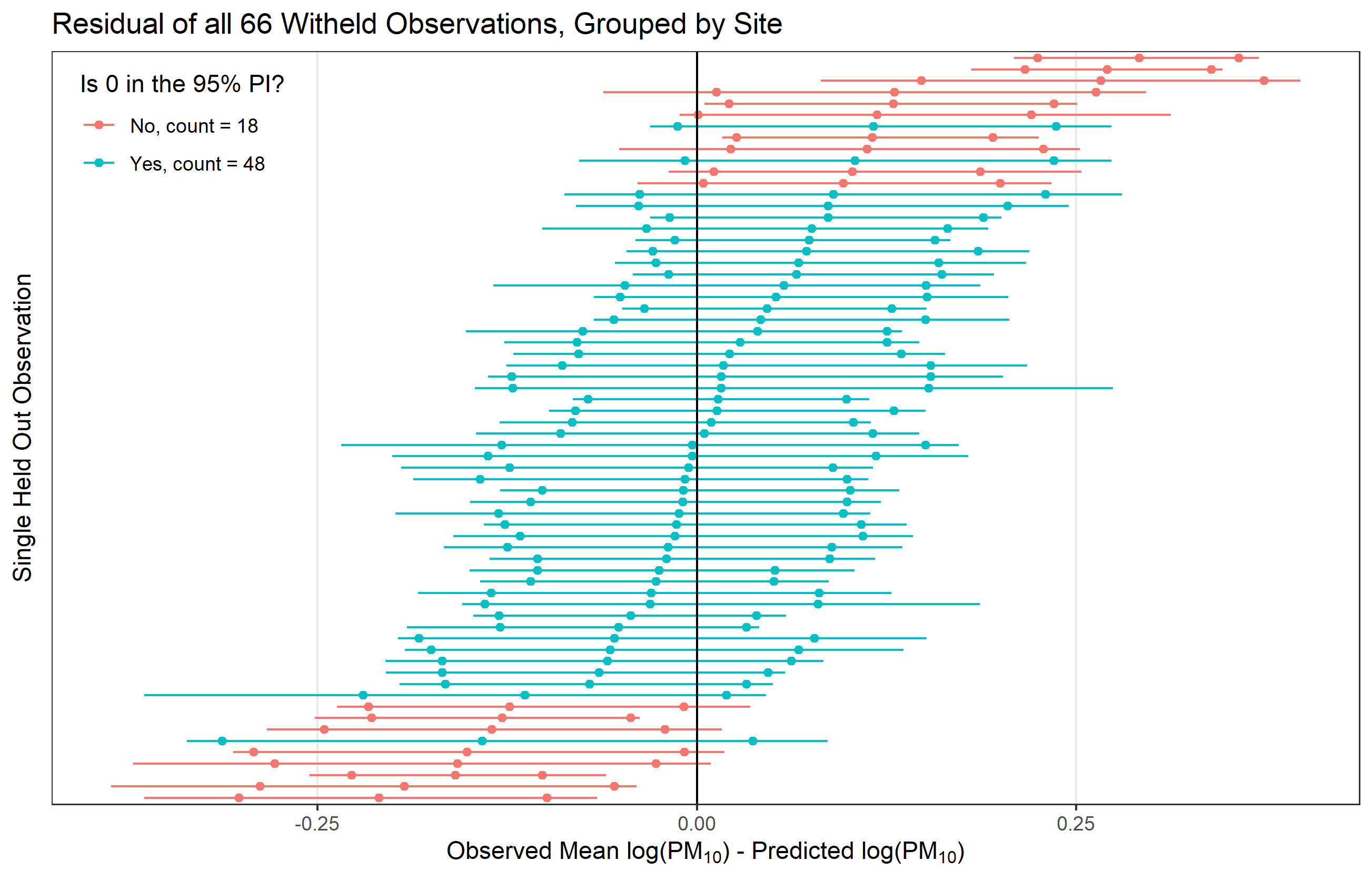
Figure 22: This shows the posterior distribution of the withheld observations, centered at 0 by subtracting them from the observed observations. For each site, the central point is the posterior mean, the left and right points are the posterior 0.025 and 0.975 percentiles respectively, and the line goes from the smallest to the largest value in the 100 samples from the posterior. It is concerning that 35% of the validation points don’t have the observed value within the 95% prediction interval, which suggests that some part of the model could be improved.

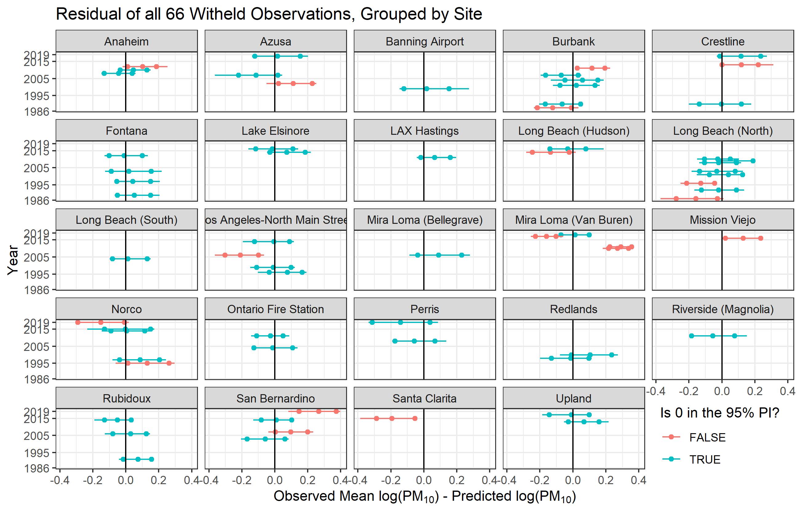
Figure 23: Here the posterior distributions shown in the previous figure are split up by site and by year in an attempt to see any patterns suggesting where the model could be improved. It looks like sites have more heterogeneity in the distribution of out-of-bounds predictions than years, so perhaps the spatial covariance function needs tweaking.

6 Preferential Sampling

As discussed in Section 4.5, PS results in sampling sites that have a stochastic dependence upon the latent field of interest and results in a biased estimation of the true field. This chapter presents evidence PS found in the course of this project.

Because the test for preferential sampling is done by comparing the location of all sites to simulated sites sampled on the pollutant field, a field calculated from all the sites. To that end, after the validation modelling that held back 10% of the data, the same model using all the data was run .

6.1 Governmental Acknowledgement of Preferential Sampling

The first and perhaps most clear-cut evidence for PS are direct statements from the agencies responsible for site selection, the SCAQMD and EPA. In their five-year reports, the SCAQMD describes some of how the monitoring locations are distributed. On page 63 of the 2010 SCAQMD 5-year report and page 83 of the 2015 version is the following statement:

“Real time monitors, for the most part, are clustered in the high concentration areas…” “Real time $PM_{10}$ monitors also support ongoing health studies in the region.”

Bermudez and Fine (2010), Bermudez et al. (2015), Miyasato et al. (2019) Site clustering is one way that PS is described, and its presence is used by Watson (2021) as an indicator for the presence of PS.

“Though the current PM 10 network is relatively stable, monitoring agencies may continue divesting of some of the PM10 monitoring stations where concentration levels are low relative to the NAAQS.”

EPA (2016) This divesting of low-concentration sites from the network is similar behavior to that found in the UK for black smoke (Zidek and Zimmerman, 2010).

6.2 Four Site Categories

In Figures 6, 5, and 7 We demonstrated the first sign of preferential sampling in the data, by examining the traces of sites grouped by when they entered and left the network. Sites were split by a 2-by-2 table based on whether a site was A) present at the start of the network or B) still monitoring at the end of the network (see table 12).

		Present in 1986
		Yes	No
Present in 2019	Yes	Continuous (many)	Added (many)
	No	Removed (2 sites)	Added then removed (3 sites)

Table 12: Naming conventions for sites categorized according to the two-way table made by whether the site is A) Present in the network in 1986, and B) Present in the network in 2019.

Calling back to those three figures, the “Continuous” and “Added then Removed” sites have very similar overall means, an increase compared to the overall mean of all sites. In contrast, the “Removed” and “Added” sites have similar means that are lower compared to the overall mean. This pattern could be a result of preferential sampling early (starting biased high, then corrected by adding low pollution sites later) or late (ending biased low, the mean dragged down by the sites added later). Alternatively, a change in the pollution field’s distribution could explain this; if the tail shifts and drags the mean over time. However, the box plots of each year do not seem to support that explanation, as they stay roughly symmetrical throughout.

Table 13 shows the result of including those four categories as fixed effects in the model

	Value	SD
WAIC	-9.532e2
DIC	-9.645e2
Intercept	-0.0004295981	31.59055710
Continuous	0.0094430558	0.12665671
Removed	-0.2024973929	0.10773814
Temporary	-0.2746064961	0.04417141
RW2	[-1.38555, -0.106361]	[31.5907, 31.5908]
Matérn	[-0.394883, 0.70015]	[0.107131, 0.427265]
Hyperpar Gaussian Prec.	82.1063483	5.363589751
Hyperpar RW2 Prec.	30.2078731	8.969724584
Hyperpar Matérn Range	28.0537004	11.325932812
Hyperpar Matérn Stdv	0.2980578	0.043042302
Hyperpar AR(1) rho	0.9948262	0.001907155

Table 13: Including fixed effects for the 4 site retention category

6.3 PStestR: A Preferential Sampling Package

As described in Section 4.6, Watson (2021) proposed a theory to detect preferential sampling. They also provide an R package called PStestR to implement the test, which is used below.

Implementation in PStestR

Having obtained a predicted pollutant surface and knowing the location of sites, the package calculates the mean of the $k$ nearest neighbors at each site and correlates that with the estimated concentration of the pollutant. The same result is produced for many Monte Carlo samples of possible sites over the whole network area. The package described in Watson (2021) can be used under two paradigms.

1. The number of nearest neighbors to use is known.

2. The number of nearest neighbors is uncertain, and testing a range of options is part of the research question.

In the first case, a single test is performed comparing the known sites to the distribution of the Monty Carlo samples. In the second case, a multiple comparison test is implemented with a comparison for each value of $k$, the number of nearest neighbors used. PStestR then provides the following outputs:

• Test Rho: The calculated Spearman’s Rho for the network during each year.

• Empirical P-Value: Compares the Test Rho for the actual network to the distribution from the Monte Carlo simulation.

Tuning Parameters

PStestR has several parameters that can be adjusted to affect the simulation and test. Here we describe those parameters and what we chose to use.

• Number of Nearest Neighbors, $k$: As described earlier, the number of nearest neighbors included in the test can be tuned to improve the power of the overall test at the cost of precision. Looking at the points showing site locations in fig 3, the largest cluster seems to be about 3. So we set $k=3$.

• Number of Monte Carlo Samples: Increasing the number of Monte Carlo samples improves the posterior’s precision at the cost of computational time. An M of 1000 is large enough to be reasonable while still being manageable by the computer on which this analysis was performed.

• Year: Each year is not independent of the others, but each test on a year will assume that it is. To avoid multiple comparisons, it is necessary to choose one year to test. We choose 2019 because it will show the current state of the network.

6.4 Results of Test

Result of Test for 2019

The network in 2019 has a correlation of -0.822 and an Empirical P-Value of 0.00300. This correlation is very close to -1 and the P-Value implies that the observed network of sites would be very unlikely to be chosen in a sampling regime that is not stochastically dependent upon the pollutant field.

Figure 24 shows the distribution of the test Rho for each of the MCMC samples and the position on that distribution of the test Rho for the actual network during 2019.

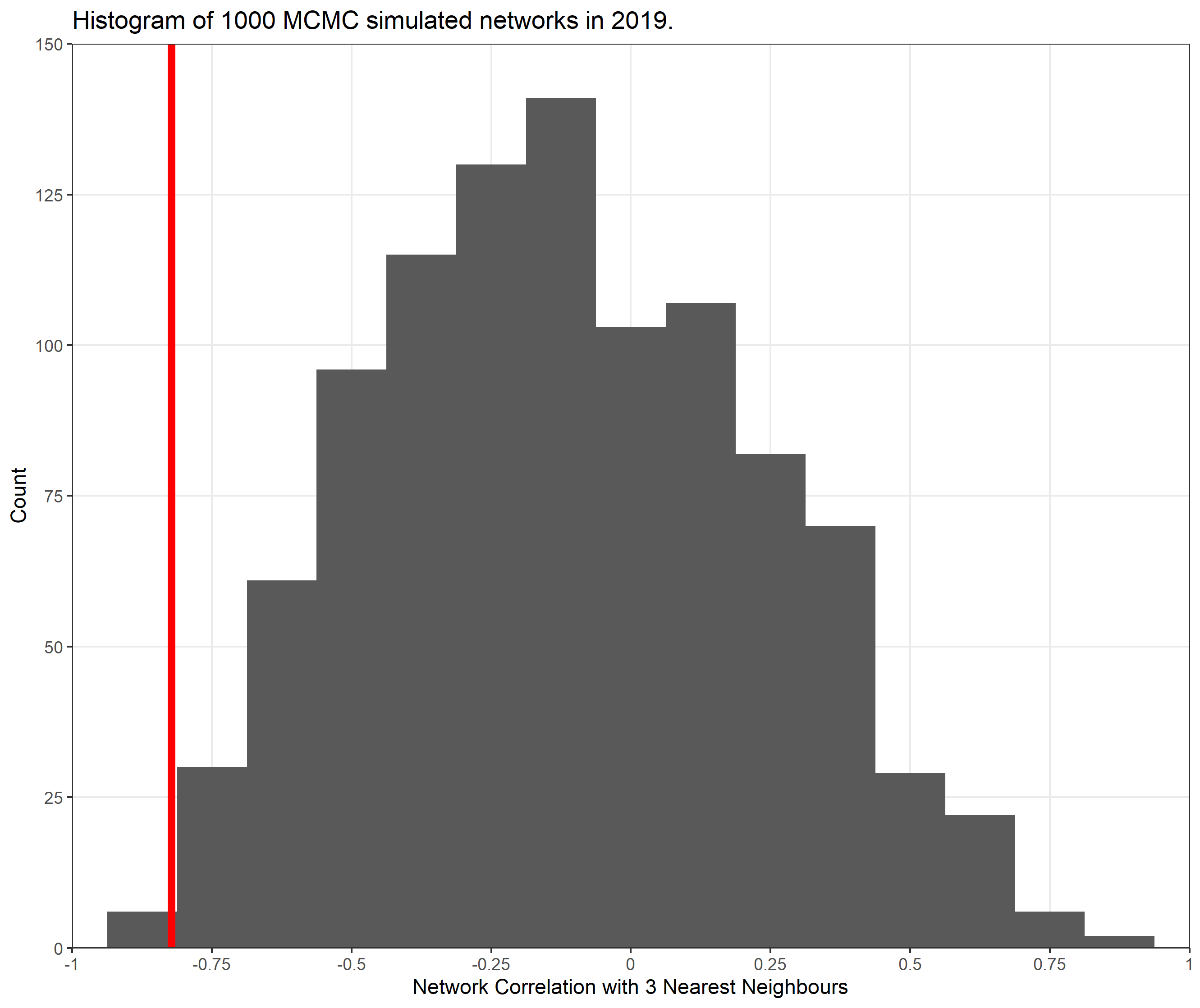
Figure 24: Histogram of sampled network Correlation of 1000 MCMC samples showing their empirical distribution. The red line shows where the observed correlation lies in relation to the samples.

Time Series of Test Score

Despite knowing there is a lack of independence between years, we chose to assess the data as a time series. What follows is a more qualitative exploration rather than a quantitative result.

Before 1994 the network did not have enough sites to produce a result from the PStestR algorithm. However, except for 1997, from 1994 to the present there are enough sites for a correlation score.

Figure 25 shows that each year has a negative correlation score, implying preferential sampling for locations with a higher concentration of $PM_{10}$. In addition, the Test Rho’s time series in the bottom half of Figure 25 shows a decrease in time, which would imply an increase in preferential sampling from earlier to later dates. On the other hand, the “trend” could easily result from a stationary time series.

To examine whether the scores can be explained by a stationary time series, ACF and PACF plots of the Test Rho (Figure 26) were produced. There are two ways of handling the missing value for 1997 while calculating the ACF and PACF: (1) interpolate the missing year; (2) cut out the time series before the missing year. We chose option (1) and so interpolated the missing year’s Test Rho by using the mean of 1996 and 1998. Figure 26 suggests the Test Rho time series is stationary, with a possible AR(1) process.

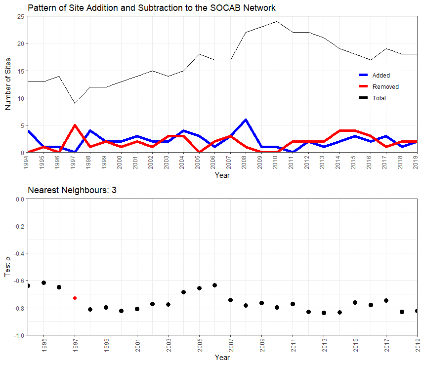
Figure 25: Top: Counts of sites in the network for each year. Total sites are in black, the number of sites that were removed compared to the previous year is in red, and several sites that were added compared to the previous year are in blue. Bottom: Test $\rho$ (Spearman’s Rank Correlation) for the three nearest neighbors. A negative correlation implies a bias towards high-concentration monitoring. 1997 had too few sites to calculate a score and is interpolated as the mean of 1996 and 1998 scores (red dot).

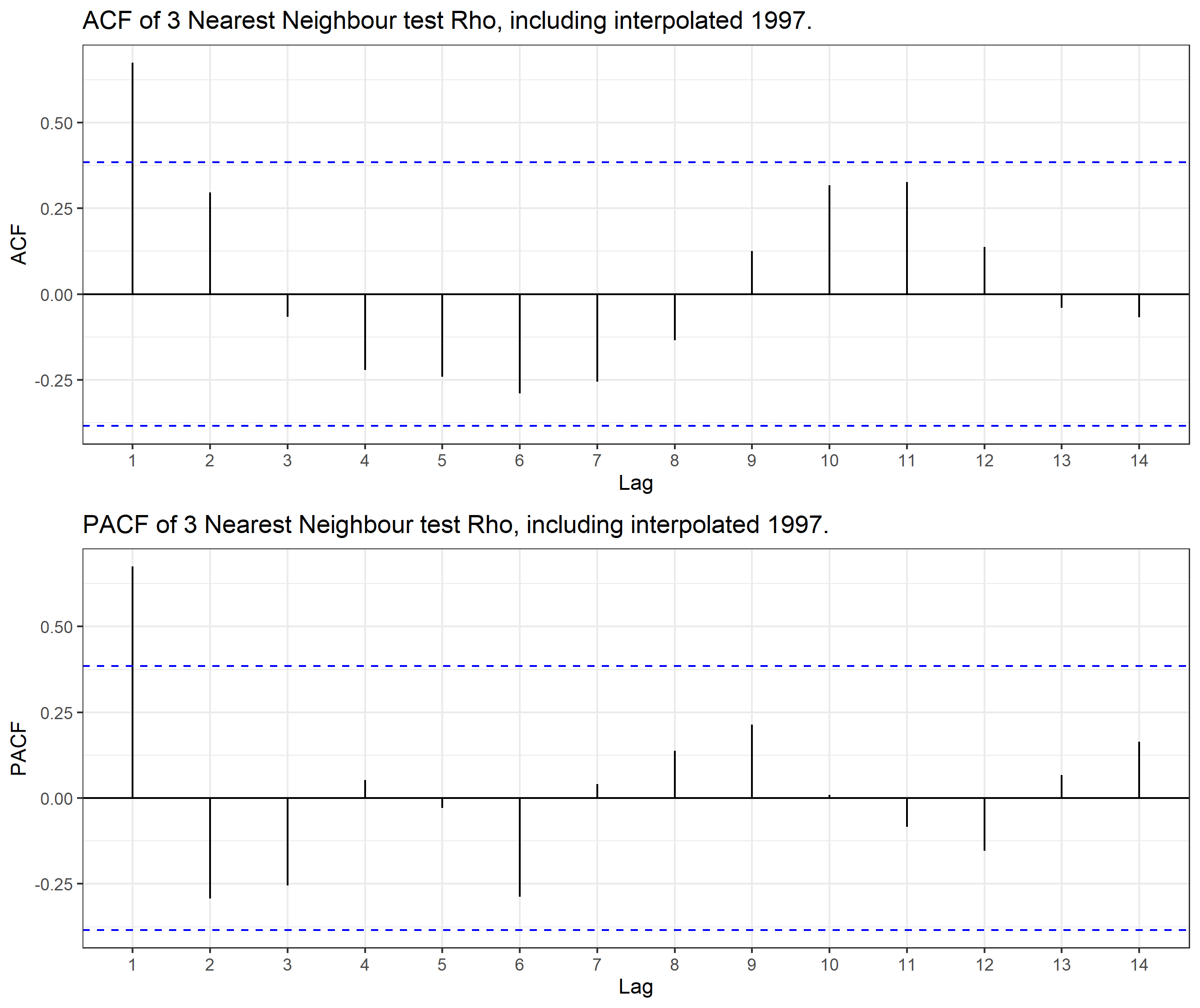
Figure 26: An examination of the autocorrelation of the nearest neighbors. With both quickly decaying, it seems unlikely that there is nonstationarity in the time series. Note that since sites carry over from year to year, each year’s correlation is not an independent observation. This uses the interpolated value for 1997 as part of the time series. With the spike in ACF and PACE at lag 1, the smooth decay in the ACF, and the sharp drop-off in the PACF, an AR(1) process seems a plausible model choice.

The final issue we investigated is whether a relationship between the Test Rho and the addition or removal of sides from the network exists, ie the dots and the red and blue lines in Figure 25. This could be another indicator of administrative choices resulting in preferential sampling over time as the network evolves. Spearman’s correlation between the time series test scores and the two-time series of network site changes was used. One correlation with the interpolated point included was done, and one with that year removed from the site counts.

	Interpolated 1997	1997 Absent
Number of Added Sites	0.02921195	0.09615902
Number of Removed Sites	-0.1937513	-0.2670485

Table 14: Spearman’s Rho between the network’s Test Rho and the number of sites added or removed from the network compared to the previous year.

Table 14 shows the results of the correlation. Adding sites seems to have very little correlation with the network’s Test Rho over the years of monitoring. Site removal has a stronger correlation, but still not much.

7 Conclusions

7.1 Presence of Preferential Sampling

This report found evidence of Preferential Sampling in the SOCAB. Government reports provided textual support, while statistical support came from both the pattern of network adjustment and the PStestR package. This PS results in observed pollution higher than the regional mean.

7.2 Complications Not Considered

Throughout this work, several ways of adding complexity were sidelined. Also, having finished, several extensions or new angles of inquiry have occurred to me. These include considerations when modelling the field, ways to interpret preferential sampling, and how to extend the work to applicability.

Modelling the field

As discussed in Section 4.9, many sites have multiple instruments recording $PM_{10}$ at the same time. These could provide an understanding of the nugget effect by being replicated measurements. However, this would require modifications to the INLA model to account for the unusual presence of information on the nugget. Therefore, the instruments were combined into a mean to simplify modelling.

Section 4.8 described how the study area to SOCAB was constrained. However, the decisions are made by the SCAQMD which has jurisdiction over a wider area. If the study domain could be extended to the jurisdictional boundary instead of the geographic airshed boundary, a fuller understanding of the preferential sampling process would be achieved. However, this requires modelling the discontinuity in the $PM_{10}$ surface.

The exploratory examination of the preferential sampling time series in Section 6.4 did not account for the lack of independence between years. It is not known what modifications would have to be made to the PStestR algorithm to account for this, but it is another area that could be examined.

Understanding Preferential Sampling

The MCMC samples of hypothetical networks generated by PStestR placed sites with a uniform distribution over the SOCAB’s area. However, sites have numerous constraints on their actual real-world location. Implementing these constraints would require finding documentation of what considerations are made for site selection, and then using a GIS tool with data layers describing those considerations. Another way to examine the network for preferential sampling is whether a given site complies with EPA standards. If decisions are being made based upon a site’s compliance or lack thereof, including it into the PS model could help understand the decisions.

Future Applicability

Much of the motivation for detecting preferential sampling is from its potential impact on studies using the observed data as an unbiased sample of population exposure. Having found evidence for Preferential Sampling, a reasonable next step could be to determine how this bias has affected various studies. A sensitivity study testing the impact of PS on health studies might help.

7.3 Workflow

We now summarize the flow of the work we learned was necessary to reach the findings reported in this report. We hope that this blueprint might be of value in future work aimed at the same objective but in a different geographical domain. Of note is an R package developed partway through this work that uses the EPA API called raqdm. This package makes data acquisition for future work more streamlined.

• Obtain EPA data, e.g. through the R package raqdm.

• Obtain a spatial shape file for the area of interest, e.g. from an online GIS service.

• Match the projection of the spatial shape file to the coordinate system of the data and then filter the data for the pollutant of interest, exclusion criteria, and area of interest.

• Perform preliminary data exploration for spatial and temporal trends, presence of anisotropy, and utility of metadata for modelling.

• Create a mesh, using the area of interest as a boundary, and preliminary range as edge lengths.

• Model the data with splines for spatial and temporal trends, Matétern function for spatial covariance and probably an AR(1) for temporal covariance.

• After validating the model, use it to predict a surface.

• Run a preferential sampling test using PStestR and the predicted surface.

References

- Bermudez and Fine [2010] Rene M Bermudez and Philip M. Fine. SOUTH COAST AIR QUALITY MANAGEMENT DISTRICT 5 YEAR NETWORK ASSESSMENT. 2010.
- Bermudez et al. [2015] Rene M Bermudez, Payam Pakbin, and Jason C Low. SOUTH COAST AIR QUALITY MANAGEMENT DISTRICT 5 YEAR NETWORK ASSESSMENT. 2015.
- Cameletti et al. [2011] M. Cameletti, F. Lindgren, D. Simpson, and H. Rue. Spatio-temporal modeling of particulate matter concentration through the spde approach. AStA Advances in Statistical Analysis, pages 1–23, 2011.
- Cressie and Wikle [2011] N. Cressie and C.K. Wikle. Statistics for spatio-temporal data, volume 465. Wiley, 2011.
- Diggle and Ribeiro [2007] P.J. Diggle and P.J. Ribeiro. Model Based Geostatistics. Springer, 2007.
- Diggle and Ribeiro Jr [2010] P.J. Diggle and P.J. Ribeiro Jr. Model based geostatistics. Springer Verlag, 2010.
- Diggle et al. [2010] P.J. Diggle, R. Menezes, and T. Su. Geostatistical inference under preferential sampling. Journal of the Royal Statistical Society: Series C (Applied Statistics), 59(2):191–232, 2010.
- EPA [2016] EPA. Integrated review plan for the national ambient air quality standards for particulate matter, 2016.
- EPA [2021] EPA. Title 40: Projection of the environment, 2021. URL https://www.law.cornell.edu/cfr/text/40/part-58.
- Fuglstad et al. [2017] Geir-Arne Fuglstad, Daniel Simpson, Finn Lindgren, and Håvard Rue. Constructing priors that penalize the complexity of gaussian random fields. Journal of the American Statistical Association, (just-accepted), 2017.
- Gómez-Rubio [2020] Virgilio Gómez-Rubio. Bayesian inference with INLA. Chapman and Hall/CRC Press, 2020. URL https://becarioprecario.bitbucket.io/inla-gitbook/index.html.
- Isaaks and Srivastava [1988] EH Isaaks and R Mohan Srivastava. Spatial continuity measures for probabilistic and deterministic geostatistics. Mathematical geology, 20(4):313–341, 1988.
- Miyasato et al. [2019] Matt Miyasato, Jason Low, and Rene M Bermudez. ANNUAL AIR QUALITY MONITORING NETWORK PLAN. 2019.
- Ott [1990] W Ott. A Physical Explanation of the Lognormality of Pollutant Concentrations. Journal of the Air Waste Management Association, 40:1378–1383, 1990.
- Righetto et al. [2020] Ana Julia Righetto, Christel Faes, Yannick Vandendijck, and Paulo Justiniano Ribeiro Jr. On the choice of the mesh for the analysis of geostatistical data using r-inla. Communications in Statistics - Theory and Methods, 49(1):203–220, 2020. %Define␣a␣command␣\doi{}␣to␣typeset␣a␣digital␣object␣identifier␣(DOI).%Note:␣if␣the␣following␣definition␣raise␣an␣error,␣then␣you␣likely%have␣an␣ancient␣version␣of␣url.sty.␣␣Either␣find␣a␣more␣recent␣version%(3.1␣or␣later␣work␣fine)␣and␣simply␣copy␣it␣into␣this␣directory,␣␣or%comment␣out␣the␣following␣two␣lines␣and␣uncomment␣the␣third.doi:10.1080/03610926.2018.1536209. URL ttps://doi.org/10.1080/03610926.2018.1536209.
- Schlather et al. [2004] Martin Schlather, Paulo J Ribeiro, and Peter J Diggle. Detecting dependence between marks and locations of marked point processes. Journal of the Royal Statistical Society: Series B (Statistical Methodology), 66(1):79–93, 2004.
- Shaddick and Zidek [2012] G. Shaddick and J. V. Zidek. Preferential sampling in long term monitoring of air pollution: a case study. Technical report, Technical Report 267, Department of Statistics, University of British Columbia, 2012.
- Shaddick and Zidek [2014] Gavin Shaddick and James V Zidek. A case study in preferential sampling: Long term monitoring of air pollution in the uk. Spatial Statistics, 9:51–65, 2014.
- Simpson et al. [2017] Daniel Simpson, Håvard Rue, Andrea Riebler, Thiago G Martins, Sigrunn H Sørbye, et al. Penalising model component complexity: A principled, practical approach to constructing priors. Statistical science, 32(1):1–28, 2017.
- Snyder [1987] John P. Snyder. Map Projections - A Working Manual. Washington, 1987.
- Watson [2021] Joe Watson. A perceptron for detecting the preferential sampling of locations and times chosen to monitor a spatio-temporal process. Spatial Statistics, 43:100500, 2021.
- Watson et al. [2019] Joe Watson, James V Zidek, Gavin Shaddick, et al. A general theory for preferential sampling in environmental networks. Annals of Applied Statistics, 13(4):2662–2700, 2019.
- Wong et al. [2004] David W Wong, Lester Yuan, and Susan A Perlin. Comparison of spatial interpolation methods for the estimation of air quality data. Journal of Exposure Science & Environmental Epidemiology, 14(5):404–415, 2004.
- Zidek et al. [2012] James Zidek, Nhu Le, and Zhong Liu. Combining data and simulated data for space–time fields: application to ozone. Environmental and Ecological Statistics, 19(1):37–56, 2012. ISSN 1352-8505. %Define␣a␣command␣\doi{}␣to␣typeset␣a␣digital␣object␣identifier␣(DOI).%Note:␣if␣the␣following␣definition␣raise␣an␣error,␣then␣you␣likely%have␣an␣ancient␣version␣of␣url.sty.␣␣Either␣find␣a␣more␣recent␣version%(3.1␣or␣later␣work␣fine)␣and␣simply␣copy␣it␣into␣this␣directory,␣␣or%comment␣out␣the␣following␣two␣lines␣and␣uncomment␣the␣third.doi:10.1007/s10651-011-0172-1.
- Zidek and Zimmerman [2010] James V Zidek and Dale L Zimmerman. Monitoring network design. Handbook of Spatial Statistics, pages 131–148, 2010.