Data as voters: instance selection using approval-based multi-winner voting

Abstract

We present a novel approach to the instance selection problem in machine learning (or data mining). Our approach is based on recent results on (proportional) representation in approval-based multi-winner elections. In our model, instances play a double role as voters and candidates. Each instance in the training set (acting as a voter) approves of the instances (playing the role of candidates) belonging to its local set (except itself), a concept already existing in the literature. We then select the election winners using a representative voting rule, and such winners are the data instances kept in the reduced training set.

1 Introduction

Instance selection (or prototype selection) [García et al.(2015)] is a preprocessing task in machine learning (or data mining) that aims at selecting a subset of the data instances composing the training set that a machine learning algorithm will use. There are two main reasons to perform this task: efficiency and cleaning. Reducing the size of the training set reduces the computational cost of running the machine learning algorithm, especially in the case of instance-based classifiers like KNN (see the Preliminaries section for a description of KNN classifiers). Furthermore, we may be interested in removing noisy instances from the training set: instances due to errors or other causes can induce mistakes in the machine learning algorithm.

[Carbonera and Abel(2018)] define instance selection as “a machine learning pre-processing task that consists in producing a smaller representative set of instances from the total available data, which can support the original task with no performance loss (or, at least, a reduced performance loss)”. This paper presents a novel approach to the instance selection problem. Our approach is to take the above statement literally and to exploit recent results of the computational social choice [Brandt et al.(2016), Conitzer(2010)] community on representation in approval-based multi-winner voting (see [Faliszewski et al.(2017)] for an overview of multi-winner voting and [Lackner and Skowron(2023)] for a survey on approval-based multi-winner voting). In our model, instances play a double role as voters and candidates. Each instance (acting as a voter) approves of the instances (playing the role of candidates) belonging to its local set (except itself, as will be discussed in Section 3), a concept already existing in the literature. We then select a committee (the winners of the election) using a representative voting rule, and such committee will be the reduced training set (the output of the instance selection process).

We then conduct two experiments to evaluate our approach. In our experiments, we follow the methodology employed in previous works [Carbonera and Abel(2018), Carbonera and Abel(2015)]. In the first experiment, we exploit representation axioms available in the state of the art to guarantee that the reduced training set would classify correctly with a KNN classifier every instance in the original training set as long as the local set of the instance contains at least three instances. In the second experiment, we evaluate our ideas with several voting rules and several values for the target committee size.

1.1 Related work

Instance selection Instance selection methods can be classified according to several criteria. The first criterion is whether the reduced training set is obtained starting with an empty set and then adding instances to it (incremental method) or starting with the whole training set and then removing instances from it (decremental method). All the voting rules we consider in this paper begin with an empty committee and therefore induce incremental methods. However, there exist voting rules in the state of the art that start with the whole set of candidates in the committee and then proceed to remove candidates until the desired target committee size is reached.

A second criterion divides instance selection methods in condensation methods, edition methods, and hybrid methods [García et al.(2015)]. Condensation methods try to keep the instances in the boundaries of each class and to remove the inner instances; edition methods try to remove noisy instances (which are often in the boundaries); finally, hybrid methods typically start applying an edition method first to remove noisy instances, and then try to remove also inner instances.

Among the condensation methods proposed in the literature, we can cite the Condensed Nearest Neighbour (CNN) [Hart(1968)] (the first condensation method proposed), the Reduced Nearest Neighbour (RNN) [Gates(1972)], Prototype Selection by Clustering (PSC) [Olvera-López et al.(2010)], Local Density Instance Selection (LDIS) [Carbonera and Abel(2015)], and Instance Selection based on Dense Spatial Partitions (ISDSP) [Carbonera and Abel(2018)]. ISDSP is, to our knowledge, the only algorithm available in the state of the art with a parameter to select the desired number of instances that should be kept in the reduced training set.

The first edition method proposed was the Edited Nearest Neighbour (ENN) [Wilson(1972)], and it is still often used as the first step in hybrid methods. Later, [Leyva et al.(2015)] proposed the Local Set-based Smoother (LSSm).

Hybrid methods have attracted great interest because they try to combine the best features of condensation and edition methods. Some prominent hybrid methods are Instance Based Learning 3 (IB3) [Aha et al.(1991)], Decremental Reduction Optimization Procedure 3 (DROP3) [Wilson and Martinez(2000)], Iterative Case Filtering (ICF) [Brighton and Mellish(2002)], and Local Set Border Selector (LSBo) [Leyva et al.(2015)].

Machine learning and voting Single-winner voting has been used in machine learning for a long time. The most common use of voting in machine learning is in ensemble methods (see, for instance [Zhou(2021)]). In ensemble methods, several classifiers are built from a given training set, and the final output is obtained by combining the outcome of each classifier. A typical algorithm to combine such outcomes is voting with a majority rule: the class selected by most classifiers is finally chosen. A particular instance of ensemble methods is the popular Random Forest classifier. To our knowledge, this is the first attempt to employ multi-winner voting in a machine learning task.

In the opposite direction, machine learning techniques have been used in computational social choice to learn voting rules. The idea here is to learn a suitable voting rule from a training set of elections and desired outcomes for such elections. Examples of this area of research are the work of [Procaccia et al.(2009)] for single-winner voting and the recent work of [Caragiannis and Fehrs(2022)] for approval-based multi-winner voting.

2 Preliminaries

2.1 Machine learning concepts

The input of the instance selection problem is a training set composed of $n$ data instances, $\mathcal{T}=\{d_{1},\ldots,d_{n}\}$. For each data instance $d_{i}$ we know a vector of $m$ features $f_{i}=(f_{i,1},\ldots,f_{i,m})\in F_{1}\times\ldots\times F_{m}$ and a class $c_{i}\in\mathcal{C}$ to which the instance belongs. The set of possible classes $\mathcal{C}$ is assumed finite and known.

Given a (reduced) training set $\mathcal{T}$, a classifier $K$ outputs a function $K(\mathcal{T}):F_{1}\times\ldots\times F_{m}\rightarrow\mathcal{C}$ that estimates the class of a new instance given its vector of features. The accuracy of a classifier can be estimated with a test set $\mathcal{T}_{s}=\{d^{s}_{1},\ldots,d^{s}_{p}\}$, that should be disjoint from the training set. For each data instance $d^{s}_{i}$ in the test set, the corresponding vector of features $f^{s}_{i}\in F_{1}\times\ldots\times F_{m}$ and class $c^{s}_{i}\in\mathcal{C}$ are also known. The accuracy of the classifier $K$ for training set $\mathcal{T}$ is then defined as $\frac{|\{d^{s}_{i}\in\mathcal{T}_{s}:K(\mathcal{T})(f^{s}_{i})=c^{s}_{i}\}|}{|\mathcal{T}_{s}|}$.

It is often the case that only a training set is available. In such cases, the accuracy of the classifier can be estimated using the so-called $k$-fold cross-validation (see [Zhou(2021)]). The data instances in the training set are randomly allocated in $k$ mutually disjoint subsets (the folds) $\mathcal{T}_{1},\ldots,\mathcal{T}_{k}$ of equal size ($k=10$ is typical). Then, we evaluate the classifier in $k$ iterations. In each iteration, one fold plays the role of the test set while the other folds play the role of the training set. The accuracy of the classifier is then computed as $\frac{\sum_{j=1}^{k}|\{d_{i}\in\mathcal{T}_{j}:K(\mathcal{T}\setminus\mathcal{T}_{j})(f_{i})=c_{i}\}|}{|\mathcal{T}|}$.

Many different classifiers exist in the state of the art (see, for instance [Zhou(2021)]). In this paper, we focus on two of them: K-Nearest Neighbours (KNN) and Support Vector Machines (SVM).

Given the vector of features of a new instance whose class is unknown, a KNN classifier computes the distance between such vector and the vectors of features of the instances in the training set. The class of the new instance is then estimated using a majority rule: the class most frequent of the K instances in the training set that are closer to the new instance is selected. The value of K is usually odd to avoid ties. Typical values are K$=1$ or K$=3$.

A detailed description of an SVM classifier’s operation is out of the scope of this paper. Informally, an SVM classifier transforms the feature space into another where the regions occupied by each class can be better separated and identifies a subset of the transformed vectors of features (the support vectors) that delimit the areas occupied by each class. For a detailed description of SVM classifiers, we refer to [Cristianini et al.(2000), Zhou(2021)].

Finally, we present the concept of local set that was first introduced by [Brighton and Mellish(2002)] and has been later used in several papers related to instance selection [Caises et al.(2011), Leyva et al.(2013), Leyva et al.(2015)]. We first introduce the concept of nearest enemy. For a given instance $d_{i}$, its nearest enemy $ne(d_{i})$ is the instance of a different class closest to $d_{i}$. Then, the local set $\ell s$ of an instance $d_{i}$ is defined as the set of instances closer to $d_{i}$ than its nearest enemy.

$$\ell s(d_{i})=\{d_{j}:d(d_{i},d_{j})<d(d_{i},ne(d_{i}))\}$$ (1)

It follows that all the instances in the local set of an instance $d_{i}$ should belong to the same class as $d_{i}$.

2.2 Social choice concepts

An approval-based multi-winner election can be represented with a tuple $(N,C,\mathcal{A},q)$, where $N=\{v_{1},\ldots,v_{n}\}$ is the set of $n$ voters, $C$ is the set of candidates, $\mathcal{A}=(A_{1},\ldots,A_{n})$ is the ballot profile, and $q$ is the target committee size. Approval voting means that voters do not order the candidates according to their preferences but select the candidates they approve of. Thus, the ballot $A_{i}$ of a voter $v_{i}$ is a subset of the set of candidates $C$.

We depart from most works on approval-based multi-winner voting by allowing the actual committee size to be less than $q$. Thus, an approval-based multi-winner voting rule $R$ takes as input an election $(N,C,\mathcal{A},q)$ and outputs a set of winners or committee $W\subseteq C$ of size less than or equal to $q$. We assume that voting rules are resolute. In our experiments, ties are broken by selecting the data instance that comes first in the training set.

We now review two representation axioms that have been proposed in the literature. EJR has been proposed by [Aziz et al.(2017)], while PJR has been proposed by [Sánchez-Fernández et al.(2017b)]. Given a positive integer $\ell\leq q$, we say that a subset of the voters $N^{*}$ is $\ell$-cohesive if $|N^{*}|\geq\ell\frac{n}{q}$ and $|\bigcap_{v_{i}\in N^{*}}A_{i}|\geq\ell$.

Definition 1.

Extended/Proportional justified representation (EJR/PJR) Consider a ballot profile $\mathcal{A}=(A_{1},\dots,A_{n})$ over a candidate set $C$ and a target committee size $q$. A set of candidates $W$ of size less than or equal to $q$ is said to provide $\ell$-extended justified representation, $\ell$-EJR (respectively $\ell$-proportional justified representation, $\ell$-PJR) for $(N,C,\mathcal{A},q)$ if there does not exist an $\ell$-cohesive set of voters $N^{*}$ such that $|A_{i}\cap W|<\ell$ for each $v_{i}\in N^{*}$ (respectively, such that $|W\cap\cup_{v_{i}\in N^{*}}A_{i}|<\ell$). We say that $W$ provides extended justified representation (EJR) for $(N,C,\mathcal{A},q)$ if it provides $\ell$-EJR for $(N,C,\mathcal{A},q)$ for all positive integer $\ell\leq q$; it provides proportional justified representation (PJR) for $(N,C,\mathcal{A},q)$ if it provides $\ell$-PJR for $(N,C,\mathcal{A},q)$ for all positive integer $\ell\leq q$. An approval-based voting rule satisfies $\ell$-EJR if for every ballot profile $\mathcal{A}$ and every target committee size $q\geq\ell$ it outputs a committee that provides $\ell$-EJR for $(N,C,\mathcal{A},q)$; it satisfies $\ell$-PJR if for every ballot profile $\mathcal{A}$ and every target committee size $q\geq\ell$ it outputs a committee that provides $\ell$-PJR for $(N,C,\mathcal{A},q)$. A rule satisfies EJR (respectively, PJR) if it satisfies $\ell$-EJR for all positive integer $\ell\leq q$ (respectively, if it satisfies $\ell$-PJR for all positive integer $\ell\leq q$).

We now introduce the voting rules that we have used in our experiments. All these rules are iterative algorithms that start with an empty set of winners and add a new candidate to the set of winners at each iteration until a stop condition is met.

The rule Equal Shares (ES), also known as Rule X, has been proposed by [Peters and Skowron(2020)]. They also proved that this rule satisfies EJR. Each voter receives at the beginning $q/n$ points that are used to add candidates to the set of winners. To add a candidate to the set of winners, it is necessary that the voters that approve of such a candidate possess at least one point altogether, and this amount will be subtracted from the points possessed by the voters that approve of the candidate that is added to the set of winners at each iteration.

Denote by $\rho_{r}(v_{i})$ the number of points possessed by voter $v_{i}$ after $r$ candidates have been added to the set of winners. Thus, $\rho_{0}(v_{i})=q/n$ for each voter $v_{i}$. At iteration $r+1$, the candidate that is added to the set of winners is the candidate $c$ that minimizes the value $\gamma_{r+1}(c)$, defined as:

$$\gamma_{r+1}(c)=\min_{x}\sum_{v_{i}:c\in A_{i}}\min\{x,\rho_{r}(v_{i})\}=1$$

The value of $\rho_{r+1}(v_{i})$ is equal to $\rho_{r}(v_{i})-\min\{\gamma_{r+1}(c),\rho_{r}(v_{i})\}$ for each voter $v_{i}$ that approves of candidate $c$ and is equal to $\rho_{r}(v_{i})$ otherwise. If, after a certain iteration, no candidate exists such that the amount of points left by the voters that approve of such candidate is at least one, the algorithm stops and outputs the candidates that have been added to the set of winners so far.

The rule Simple EJR (SEJR) [Sánchez-Fernández et al.(2017a)] is an extreme case of the EJR Exact family of voting rules [Aziz et al.(2018)]. All the rules in this family satisfy EJR. At each iteration, for each candidate $c$ in $C\setminus W$, SEJR computes the plausibility $p(c)$ of such candidate. Given a (partial) set of winners $W$, the plausibility $p(c)$ of a candidate $c$ is the maximum value such that a group of voters $N^{*}$ exists satisfying (i) $c$ belongs to $A_{i}$ for all $v_{i}$ in $N^{*}$; (ii) $|N^{*}|\frac{q}{n}\geq p(c)$; and (iii) $|A_{i}\cap W|<p(c)$ for all $v_{i}$ in $N^{*}$. SEJR selects at each iteration the candidate $c$ with maximum plausibility until the plausibility of all the remaining candidates is $0$.

The last rule that we are going to consider is seq-Phragmén (SeqP) [Phragmén(1894)], proposed by the Swedish mathematician Lars Edvard Phragmén at the end of the nineteenth century (see [Janson(2016)] for an overview on Phragmén rules). SeqP is based on the notion of load: each candidate added to the set of winners induces a unit of load that must be supported among the voters that approve of such candidate. At each iteration, the candidate that is chosen is the one that minimizes the maximum voter load. Let $x^{j}_{i}$ be the load of voter $v_{i}$ after the first $j$ candidates have been added to the set of winners ($x^{0}_{i}=0$ for each voter $v_{i}$). After $j$ candidates have been added to the set of winners, the load $s^{j+1}_{c}$ that must be supported by each voter $v_{i}$ that approves of candidate $c$ in $C\setminus W$ if $c$ is added to the set of winners is

$$s^{j+1}_{c}=\frac{1+\sum_{v_{i}:c\in A_{i}}x^{j}_{i}}{|\{v_{i}:c\in A_{i}\}|}$$ (2)

The candidate $c$ with lower $s^{j+1}_{c}$ is added to the set of winners. Then, the load of the voters is updated as follows. $x^{j+1}_{i}=s^{j+1}_{c}$ for each voter $v_{i}$ that approves of $c$, and $x^{j+1}_{i}=x^{j}_{i}$ otherwise. The algorithm continues until exactly $q$ candidates have been added to the set of winners.

[Brill et al.(2017)] proved that SeqP satisfies PJR but it fails EJR.

dataset	instances	attributes	classes
cardiotocography	2126	21	10
diabetes	768	8	2
ecoli	336	7	8
glass	214	9	7
heart-statlog	270	13	2
ionosphere	351	34	2
iris	150	4	3
landsat	4435	36	6
letter-recognition	20000	16	26
optdigits	5620	64	10
page-blocks	5473	10	5
parkinson	195	22	2
segment	2310	18	7
spambase	4601	57	2
wine	178	13	3

Table 1: Datasets used in the experiments

dataset	DROP3	ENN	ICF	LSBo	LSSm	LDIS	ISDSP
cardiotocography	0.64	0.67	0.64	0.62	0.67	0.62	0.59
diabetes	0.75	0.77	0.76	0.75	0.77	0.75	0.73
ecoli	0.81	0.82	0.78	0.74	0.83	0.77	0.78
glass	0.47	0.49	0.49	0.42	0.55	0.50	0.51
heart-statlog	0.81	0.83	0.79	0.81	0.84	0.81	0.78
ionosphere	0.81	0.87	0.58	0.45	0.88	0.84	0.86
iris	0.94	0.96	0.73	0.47	0.96	0.81	0.80
landsat	0.86	0.87	0.85	0.85	0.87	0.84	0.84
letter-recognition	0.80	0.84	0.75	0.73	0.84	0.75	0.74
optdigits	0.98	0.98	0.97	0.98	0.99	0.96	0.97
page-blocks	0.93	0.94	0.93	0.92	0.94	0.94	0.91
parkinson	0.85	0.87	0.85	0.82	0.87	0.82	0.85
segment	0.91	0.92	0.91	0.80	0.91	0.89	0.88
spambase	0.90	0.90	0.90	0.90	0.90	0.89	0.87
wine	0.93	0.95	0.94	0.96	0.97	0.94	0.93
average	0.83	0.84	0.79	0.75	0.85	0.81	0.80

Table 2: Accuracy results reported by [Carbonera and Abel(2018)] with an SVM classifier

3 A social choice model for instance selection

Given a training set $\mathcal{T}=\{d_{1},\ldots,d_{n}\}$, we build an approval-based multi-winner election $(N,C,\mathcal{A},q)$ as follows. The set of voters $N$ and the set of candidates $C$ are set to $\mathcal{T}$. The ballot $A_{i}$ of each voter $d_{i}$ is set to its local set excluding $d_{i}$, $A_{i}=\ell s(d_{i})\setminus\{d_{i}\}$. We forbid data instances to approve of themselves to avoid a data instance that does not belong to the local set of any other instance (and, therefore, it is likely to be a noisy instance) being added to the set of winners. Finally, $q$ is a positive integer parameter whose value can be freely chosen.

The reduced training set $\mathcal{T}_{r}$ is then computed with voting rule $R$ as the set of winners that $R$ outputs for election $(\mathcal{T},\mathcal{T},\mathcal{A},q)$.

$$\mathcal{T}_{r}=R(\mathcal{T},\mathcal{T},\mathcal{A},q)$$ (3)

dataset	DROP3	ENN	ICF	LSBo	LSSm	LDIS	ISDSP
cardiotocography	0.63	0.64	0.57	0.55	0.67	0.54	0.50
diabetes	0.72	0.72	0.72	0.73	0.72	0.68	0.65
ecoli	0.84	0.84	0.79	0.79	0.86	0.82	0.82
glass	0.63	0.63	0.64	0.54	0.71	0.62	0.55
heart-statlog	0.67	0.64	0.63	0.66	0.66	0.67	0.63
ionosphere	0.82	0.83	0.82	0.88	0.86	0.85	0.85
iris	0.97	0.97	0.95	0.95	0.96	0.95	0.95
landsat	0.88	0.90	0.83	0.86	0.90	0.87	0.86
letter-recognition	0.88	0.92	0.80	0.73	0.93	0.79	0.71
optdigits	0.97	0.98	0.91	0.91	0.98	0.95	0.94
page-blocks	0.95	0.96	0.93	0.94	0.96	0.94	0.77
parkinson	0.86	0.88	0.83	0.85	0.85	0.74	0.79
segment	0.92	0.94	0.87	0.83	0.94	0.88	0.89
spambase	0.79	0.81	0.79	0.81	0.82	0.75	0.77
wine	0.69	0.66	0.66	0.74	0.71	0.69	0.75
average	0.82	0.82	0.78	0.79	0.83	0.78	0.76

Table 3: Accuracy results reported by [Carbonera and Abel(2018)] with a KNN classifier

dataset	DROP3	ENN	ICF	LSBo	LSSm	LDIS	ISDSP
cardiotocography	0.70	0.32	0.71	0.69	0.14	0.86	0.90
diabetes	0.77	0.31	0.85	0.76	0.13	0.90	0.90
ecoli	0.72	0.17	0.87	0.83	0.09	0.92	0.90
glass	0.75	0.35	0.69	0.70	0.13	0.90	0.90
heart-statlog	0.74	0.35	0.78	0.67	0.15	0.93	0.90
ionosphere	0.86	0.15	0.96	0.81	0.04	0.91	0.90
iris	0.70	0.04	0.61	0.92	0.05	0.87	0.90
landsat	0.72	0.10	0.91	0.88	0.05	0.92	0.90
letter-recognition	0.68	0.05	0.80	0.84	0.04	0.82	0.90
optdigits	0.72	0.01	0.93	0.92	0.02	0.92	0.90
page-blocks	0.71	0.04	0.95	0.96	0.03	0.87	0.90
parkinson	0.72	0.15	0.80	0.87	0.11	0.83	0.90
segment	0.68	0.05	0.79	0.90	0.05	0.83	0.90
spambase	0.74	0.19	0.79	0.82	0.10	0.82	0.90
wine	0.80	0.30	0.82	0.75	0.11	0.88	0.90
average	0.73	0.17	0.82	0.82	0.08	0.88	0.90

Table 4: Reduction results reported by [Carbonera and Abel(2018)]

dataset	NoR	SEJR-2	S2EJR-2	ES-2	SEJR-0.25	S2EJR-0.25	ES-0.25	SeqP-0.9	SeqP-0.1
cardiotocography	0.78	0.77	0.76	0.76	0.62	0.63	0.64	0.78	0.67
diabetes	0.77	0.77	0.76	0.76	0.76	0.77	0.77	0.77	0.76
ecoli	0.83	0.82	0.83	0.82	0.77	0.74	0.77	0.82	0.76
glass	0.54	0.54	0.49	0.47	0.46	0.46	0.46	0.49	0.46
heart-statlog	0.85	0.83	0.81	0.82	0.69	0.65	0.74	0.83	0.76
ionosphere	0.88	0.85	0.78	0.86	0.83	0.83	0.84	0.88	0.84
iris	0.97	0.97	0.89	0.96	0.86	0.84	0.91	0.96	0.83
landsat	0.87	0.87	0.86	0.87	0.85	0.84	0.85	0.87	0.85
letter-recognition	0.82	0.82	0.75	0.82	0.75	0.71	0.77	0.82	0.73
optdigits	0.98	0.98	0.97	0.98	0.95	0.95	0.97	0.98	0.95
page-blocks	0.93	0.94	0.93	0.94	0.93	0.93	0.94	0.94	0.94
parkinson	0.87	0.86	0.82	0.86	0.85	0.82	0.84	0.86	0.87
segment	0.93	0.93	0.92	0.93	0.87	0.87	0.88	0.92	0.85
spambase	0.90	0.92	0.90	0.91	0.90	0.90	0.89	0.91	0.89
wine	0.98	0.97	0.97	0.96	0.65	0.65	0.72	0.98	0.71
average	0.86	0.86	0.83	0.85	0.78	0.77	0.80	0.85	0.79

Table 5: Accuracy results obtained in our experiments with an SVM classifier

dataset	NoR	SEJR-2	S2EJR-2	ES-2	SEJR-0.25	S2EJR-0.25	ES-0.25	SeqP-0.9	SeqP-0.1
cardiotocography	0.74	0.69	0.69	0.70	0.52	0.52	0.53	0.72	0.56
diabetes	0.69	0.69	0.71	0.68	0.71	0.71	0.72	0.70	0.73
ecoli	0.85	0.86	0.86	0.87	0.78	0.78	0.78	0.86	0.76
glass	0.69	0.64	0.67	0.64	0.55	0.55	0.56	0.65	0.58
heart-statlog	0.65	0.66	0.66	0.66	0.63	0.65	0.62	0.66	0.64
ionosphere	0.84	0.85	0.87	0.84	0.84	0.86	0.84	0.84	0.83
iris	0.96	0.97	0.97	0.97	0.93	0.93	0.91	0.97	0.93
landsat	0.91	0.89	0.89	0.90	0.87	0.86	0.87	0.90	0.86
letter-recognition	0.96	0.95	0.94	0.95	0.88	0.88	0.89	0.95	0.84
optdigits	0.99	0.98	0.98	0.99	0.96	0.97	0.98	0.98	0.96
page-blocks	0.96	0.96	0.95	0.96	0.94	0.94	0.94	0.96	0.93
parkinson	0.88	0.83	0.83	0.89	0.82	0.78	0.81	0.89	0.76
segment	0.96	0.94	0.94	0.95	0.86	0.86	0.88	0.94	0.84
spambase	0.81	0.79	0.79	0.80	0.75	0.74	0.74	0.81	0.74
wine	0.73	0.72	0.71	0.68	0.68	0.70	0.69	0.65	0.68
average	0.84	0.83	0.83	0.83	0.78	0.78	0.78	0.83	0.78

Table 6: Accuracy results obtained in our experiments with a KNN classifier

4 Experimental setting

In our experiments, we follow the typical methodology used in previous works like [Leyva et al.(2015), Carbonera and Abel(2015), Carbonera and Abel(2018)] and others. We use 10-fold cross-validation. Each dataset is divided into ten equal-size folds. One fold will be used for testing, and the other nine will be the initial training set. Then, we build an approval-based multi-winner election with the instances in the initial training set and run an approval-based multi-winner voting rule to compute the reduced training set. The reduced training set is then used to train a classifier, and the accuracy of the classifier is computed by using the testing fold. The process is repeated ten times so that each fold plays the testing role once. The final accuracy is computed as described in the Preliminaries section.

We also measured the reduction achieved in each experiment, measured as reduction$=\frac{|\mathcal{T}|-|\mathcal{T}_{r}|}{|\mathcal{T}|}$, and averaging the reduction values obtained on each iteration of the 10-fold cross-validation.

We compare the results obtained in our experiments with those obtained by [Carbonera and Abel(2018)] for seven prominent instance selection algorithms: DROP3, ENN, ICF, LSBo, LSSm, LDIS, and ISDSP. In our experiments, we use the same 15 datasets (see Table 1), the same distance (the Euclidean distance) and evaluate the accuracy of the reduced training sets with the same classifiers adjusted with the same parameters as in the work of [Carbonera and Abel(2018)].

All the datasets have been obtained from the UCI Machine Learning Repository [Dua and Graff(2017)]. All the features used in all the datasets are numerical. The classifiers used are a KNN classifier with K$=3$ and an SVM classifier. We used the Weka implementation of SVM with the standard parametrization: c $=1.0$, tolerance parameter $=0.001$, epsilon $=10^{-12}$, using a polynomial kernel and a multinomial logistic regression model with a ridge estimator as calibrator. The only difference with the experiments of [Carbonera and Abel(2018)] is that we used Weka 3.9.6 with the Python Weka wrapper, while they used Weka 3.8.

For comparison purposes, we provide in Tables 2 to 4 the accuracy with the KNN and SVM classifiers and the reduction results reported by [Carbonera and Abel(2018)]. In the tables reported by [Carbonera and Abel(2018)], the ISDSP algorithm is executed with a reduction parameter fixed to $0.90$. Both for the accuracy and the reduction tables, we highlight in bold face the algorithm(s) that provide better values (considering both the algorithms studied by [Carbonera and Abel(2018)] and the results that will be shown later in our experiments) for each dataset, and for the average values obtained with all datasets.

dataset	SEJR-2	S2EJR-2	ES-2	SEJR-0.25	S2EJR-0.25	ES-0.25	SeqP-0.9	SeqP-0.1
cardiotocography	0.32	0.52	0.23	0.95	0.95	0.93	0.10	0.90
diabetes	0.44	0.58	0.31	0.95	0.95	0.93	0.10	0.90
ecoli	0.39	0.67	0.17	0.93	0.95	0.88	0.10	0.90
glass	0.32	0.56	0.24	0.93	0.95	0.92	0.10	0.90
heart-statlog	0.51	0.59	0.42	0.97	0.97	0.96	0.10	0.90
ionosphere	0.36	0.81	0.21	0.87	0.95	0.83	0.10	0.90
iris	0.15	0.82	0.02	0.83	0.94	0.80	0.10	0.90
landsat	0.31	0.78	0.09	0.88	0.96	0.82	0.10	0.90
letter-recognition	0.24	0.75	0.04	0.87	0.93	0.81	0.10	0.90
optdigits	0.34	0.88	0.01	0.88	0.97	0.78	0.10	0.90
page-blocks	0.17	0.90	0.04	0.86	0.97	0.78	0.10	0.90
parkinson	0.20	0.65	0.11	0.90	0.92	0.87	0.10	0.90
segment	0.17	0.79	0.03	0.87	0.94	0.81	0.10	0.90
spambase	0.34	0.62	0.19	0.92	0.94	0.89	0.10	0.90
wine	0.29	0.63	0.23	0.91	0.97	0.90	0.10	0.90
average	0.30	0.70	0.15	0.90	0.95	0.86	0.10	0.90

Table 7: Reduction results obtained in our experiments

5 Experiment I: a prudent approach

An interesting feature shared both by ES and SEJR is that they provide incomplete committees: given an approval-based multi-winner election $(N,C,\mathcal{A},q)$, they usually output committees of size less than $q$. In fact, it is possible to compute the winning committee with ES or SEJR for elections in which the target committee size $q$ is an arbitrary positive integer, even if $q$ is strictly greater than the number of candidates that participate in the election.

Following the ideas of [Hart(1968)] we set $q=2n$. This guarantees that every single voter that approves of at least two candidates is a $2$-cohesive group of voters and, therefore, that the winning committee computed with any voting rule that satisfies $2$-PJR (and therefore, the same holds for any voting rule that satisfies $2$-EJR or PJR or EJR) will contain at least two of the preferred candidates of such voters. This, in turn, implies that when computing the reduced training set with a rule that satisfies $2$-PJR, every instance whose local set contains at least three instances (including itself) will have at least two of the instances of its local set in the reduced training set. Therefore, any such instance will be correctly classified by using the reduced training set with a KNN classifier with K$=3$ because at least two of the three closer instances to such instance in the reduced training set will be of its class.

We also used a variant of SEJR that we have called Simple 2-EJR (S$2$EJR). The only difference between SEJR and S$2$EJR is that in S$2$EJR condition (iii) in the definition of plausibility is (iii) $|A_{i}\cap W|<\min\{p(c),2\}$ for all $v_{i}$ in $N^{*}$. In words, in S$2$EJR any voter that already has two of their preferred candidates in the winning set is considered satisfied. Therefore, such voters do not participate in the computation of the plausibility of a candidate. S$2$EJR fails EJR, but satisfies $2$-EJR. The proof can be found in the appendix.

The results obtained in our experiments are shown in Tables 5 to 7. The labels indicate the voting rule used and the value of $q/n$, separated with a hyphen. For instance, SEJR-$2$ means results obtained with the rule SEJR and $q/n=2$. Therefore, the results of Experiment I are shown in the columns labeled SEJR-$2$, S$2$EJR-$2$, and ES-$2$. We also report the accuracy values obtained with the original training sets without any reduction in the columns labeled ’NoR’ (no reduction). This information was not reported in the paper of [Carbonera and Abel(2018)]. The columns labeled ’NoR’ have not been taken into account to select the cells highlighted in bold face.

6 Experiment II: several values of $q/n$ for all rules

In this experiment, we compute reduced training sets using several values of $q/n$ and all the rules we consider in this paper. For SEJR, S$2$EJR, and ES, we compute reduced training sets for $q/n=1.75,1.5,1.25,1,0.75,0.5,$ and $0.25$. SeqP always outputs a committee of size $q$; therefore, it is impossible to compute reduced training sets with SeqP using a value of $q$ greater than $n$. Furthermore, since the committee size with SeqP is fixed given $q$, the reduction value with this rule is given by $1-q/n$. Consequently, we computed reduced training sets with SeqP for $q/n=0.9,0.8,0.7,0.6,0.5,0.4,0.3,0.2,$ and $0.1$.

Figure 1: Plot of the average values of accuracy and reduction for several values of $q/n$ with an SVM classifier

Figure 2: Plot of the average values of accuracy and reduction for several values of $q/n$ with a KNN classifier

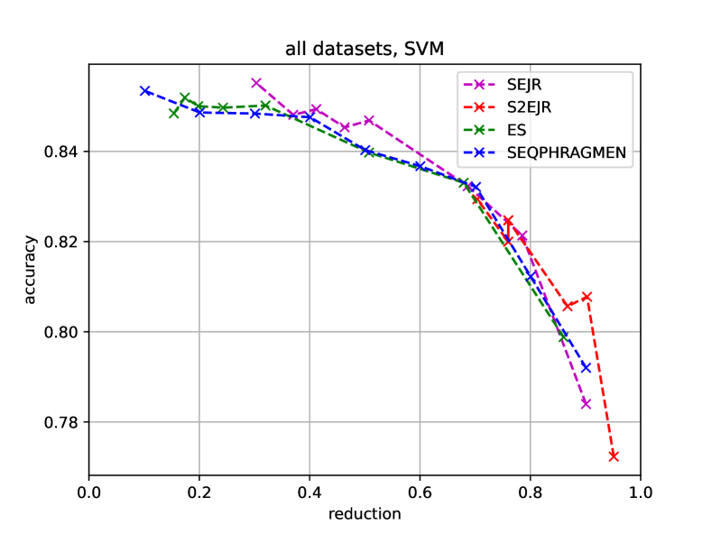
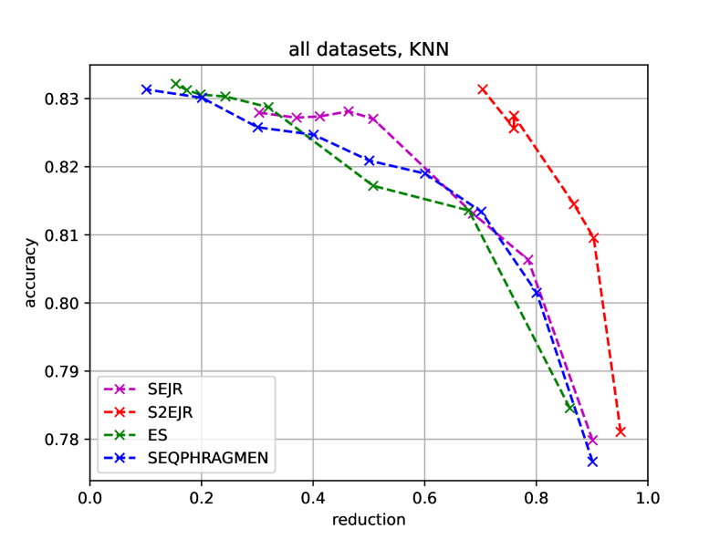
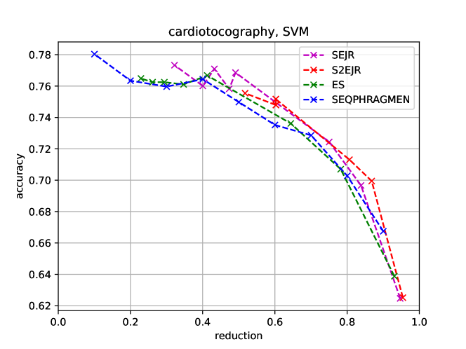
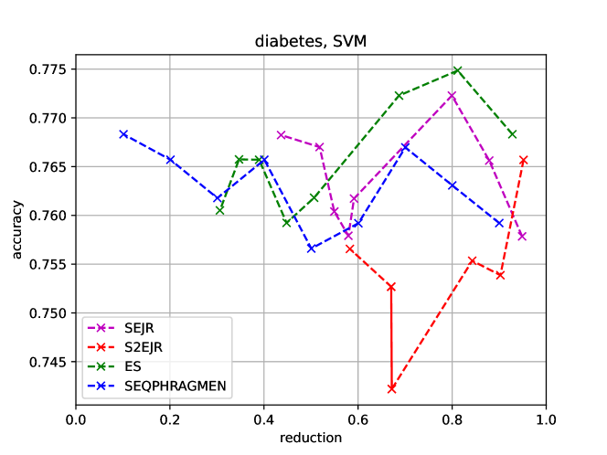
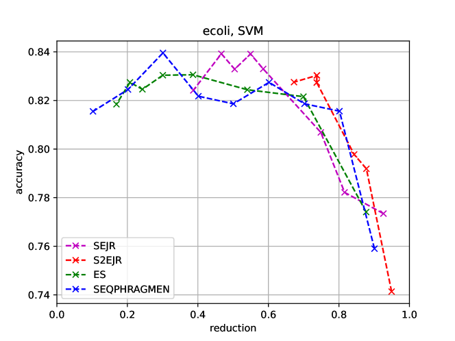
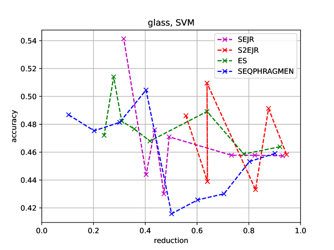
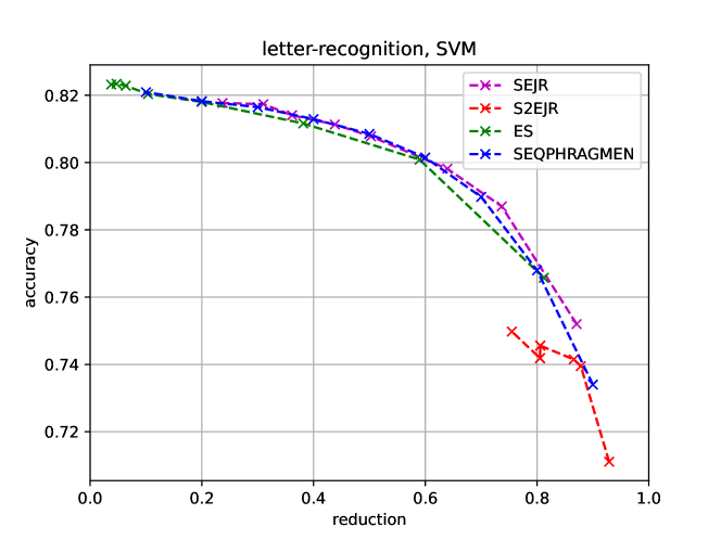
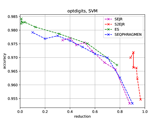
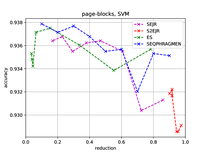
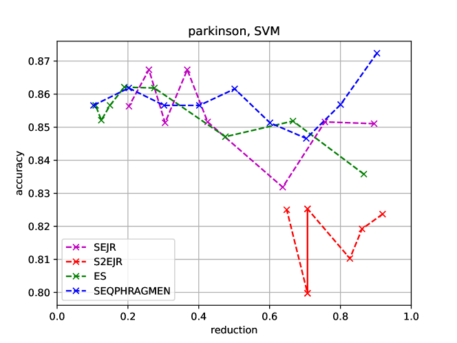
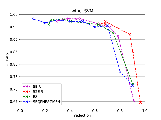
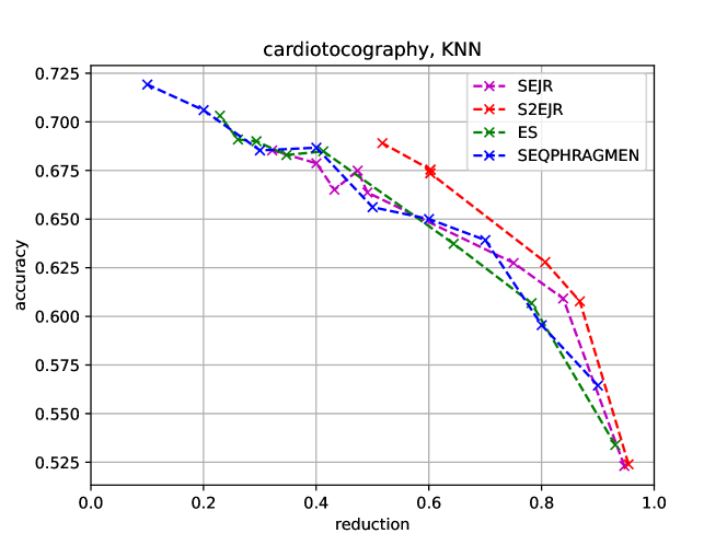
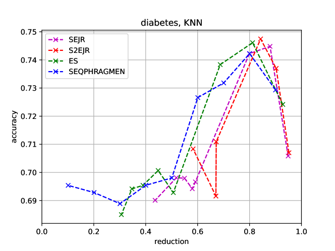
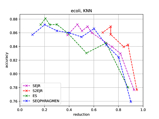
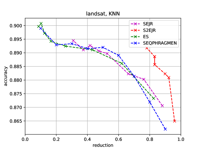
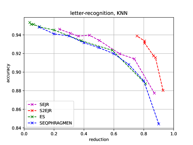
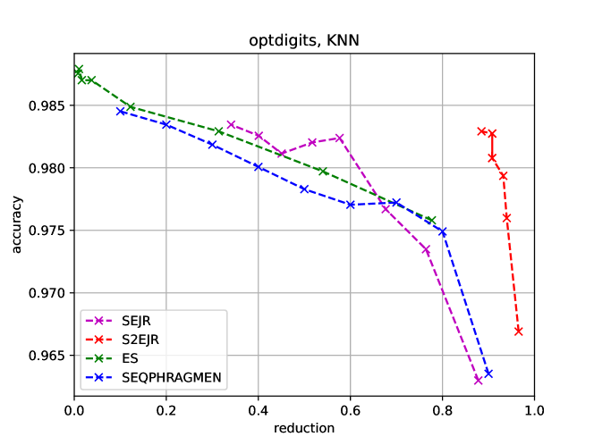
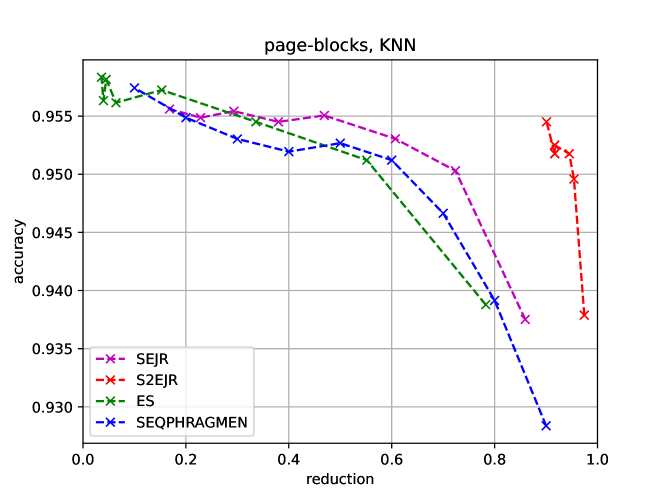
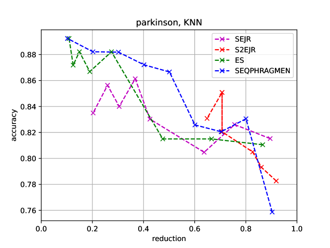
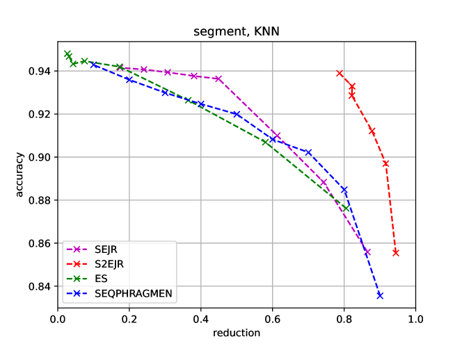
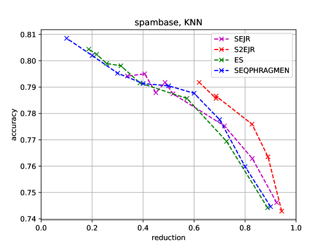
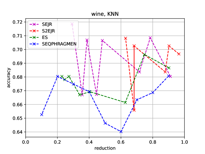
Figures 1 and 2 show the average values of accuracy and reduction for the voting rules and values of $q/n$ that have been considered in this paper. The corresponding figures for each dataset can be found in the appendix. We also include in Tables 5 to 7 the results for SeqP and $q/n=0.9$, and the results for the smallest values of $q/n$ ($0.25$ for SEJR, S$2$EJR, and ES, and $0.1$ for SeqP).

7 Discussion

We believe that the results that we have obtained in our experiments validate the proposed approach. When using high values of $q/n$, SEJR, ES, and SeqP get accuracy results competitive with those of the edition methods both for SVM and KNN classifiers. Furthermore, SEJR with $q/n=2$ obtains reduction values significantly higher than ENN and LSSm (about twice the reduction on average for ENN and nearly three times for LSSm).

For KNN classifiers, the results of S$2$EJR outperform those of the other voting rules and the algorithms studied by [Carbonera and Abel(2018)] (see Figure 2 and Table 3). For $q/n=2$, S$2$EJR achieves an impressive reduction on average of $0.70$ with no appreciable accuracy loss on average compared to the edition methods.

In the case of SVM classifiers, the advantage of S$2$EJR compared to the other voting rules is less clear. However, S$2$EJR is still competitive compared to the results reported by [Carbonera and Abel(2018)] for high reduction algorithms available in the state of the art (see Figure 1 and Table 2). However, it could be better in terms of accuracy when compared to the edition methods.

It should be noted that, as observed by [Leyva et al.(2015)], instances that are close to a class border usually have a shorter distance to their nearest enemies than inner instances. This, in turn, implies that the local sets of border instances tend to occupy smaller areas and contain fewer instances than the local sets of inner instances. Moreover, since the instances in the local set of a border instance are concentrated in a small area, they are likely also to be border instances. Thus, the reduced training set obtained with a representative multi-winner voting rule cannot contain (at least for high values of $q/n$) only inner instances because the border instances would be unrepresented in that case. This may explain why the voting rules tested in this paper also behave well with classifiers that work by identifying the class borders, such as SVM.

Another advantage of our approach is that it is possible to control the desired level of reduction by adjusting the value of the parameter $q$. To our knowledge, the only other algorithm proposed in the literature with the same property is ISDSP.

SeqP is quite different from ES and SEJR. We have already seen that ES and SEJR usually output incomplete committees while the size of the committee that SeqP outputs is always equal to $q$. Furthermore, SeqP follows a different representation paradigm than ES and SEJR. SeqP is a greedy algorithm of another voting rule also proposed by the Swedish mathematician Lars Edvard Phragmén called max-Phragmén. max-Phragmén, in addition to PJR, also satisfies another representation axiom due to [Sánchez-Fernández et al.(2017b)] called Perfect Representation (PR). [Sánchez-Fernández et al.(2017b)] proved that PR and EJR are incompatible: no rule can satisfy PR and EJR at the same time. Therefore, rules that satisfy PJR and PR or that satisfy PJR and are greedy algorithms for other voting rules that satisfy PJR and PR (like SeqP) follow a different model of representation from those that satisfy EJR.

From that perspective, it would be interesting to identify which of these representation models fits better with the problem of instance selection. However, the results we have obtained are inconclusive in this respect because SeqP performs reasonably similarly to SEJR and ES, as shown in Figures 1 and 2. The better performance shown by S$2$EJR and, to a lesser extent, by SEJR, compared to SeqP, could be explained by their ability to compute small committees that still satisfy $2$-EJR (or EJR). In any case, we believe it would be interesting to identify a voting rule that follows the PJR-PR representation model and outputs small committees (but still satisfies $2$-PJR) and to test such a rule for instance selection.

The results presented in this paper also have an interest in the computational social choice field. First, our experiments consistently show that SEJR outputs smaller committees than ES. Second, the model we have used in this paper could be exploited to build elections that could be used to make experiments of interest in computational social choice. Finally, the relationship between our work and a body of research in multi-winner voting based on placing voters and candidates as points in a metric space [Elkind et al.(2017), Pierczynski and Skowron(2019)] is worth mentioning.

Appendix A Results for S$2$EJR

We first prove that S$2$EJR always outputs a committee of size less than or equal to $q$.

Lemma 1.

For any approval-based multi-winner election $(N,C,\mathcal{A},q)$, the rule S$2$EJR always outputs a committee of size less than or equal to $q$.

Proof.

We divide the operation of S$2$EJR into two parts: (i) iterations in which the maximum plausibility $p(c)$ is greater than or equal to $2$ for some candidate $c$; and (ii) iterations in which the maximum plausibility is equal to $1$.

At each iteration of part (i), a candidate is added to the set of winners such that (a) it is approved of by a set of voters $N^{*}$ of size at least $2\frac{n}{q}$; and (b) each voter in $N^{*}$ approves of at most one of the candidates that have already been added to the set of winners. This implies that each voter can belong to $N^{*}$ at most twice in the iterations corresponding to part (i). Suppose that part (i) comprises $j$ iterations. Then, at the end of part (i), the total number of voters that approve of at least one of the candidates in the set of winners is at least,

$$\frac{j2\frac{n}{q}}{2}=j\frac{n}{q}\leq n$$

.

This proves that $j$ is not greater than $q$. Now, at each iteration of part (ii), a candidate is added to the set of winners such that (a) it is approved of by a set of voters $N^{*}$ of size at least $\frac{n}{q}$; and (b) each voter in $N^{*}$ does not approve of any of the candidates that have already been added to the set of winners. This implies that such voters can belong to $N^{*}$ at most once in the iterations corresponding to part (ii). Suppose that part (ii) comprises $h$ iterations. Then, the total number of voters that belong to $N^{*}$ in some iteration of part (ii) is, at least,

$$\frac{h\frac{n}{q}}{1}=h\frac{n}{q}\leq n-j\frac{n}{q}$$

.

This implies that $h+j\leq q$.

∎

Lemma 2.

S$2$EJR satisfies $2$-EJR.

Proof.

It is straightforward to prove the S$2$EJR satisfies $2$-EJR. For the sake of contradiction, suppose that for a certain approval-based multi-winner election $(N,C,\mathcal{A},q)$, with $q\geq 2$, the set of winners $W$ that S$2$EJR outputs does not satisfy $2$-EJR. This implies that there must exist a set of voters $N^{*}$ such that $|N^{*}|\geq 2\frac{n}{q}$, $|\bigcap_{v_{i}\in N^{*}}A_{i}|\geq 2$, but $|A_{i}\cap W|<2$ for each voter $v_{i}$ in $N^{*}$. Furthermore, a candidate $c$ must exist such that $c$ belongs to $A_{i}$ for each voter $v_{i}$ in $N^{*}$, but $c$ does not belong to $W$. According to the definition of plausibility for S$2$EJR, the set $N^{*}$ fulfills all the requirements so that the plausibility of candidate $c$ would be at least $2$. This is a contradiction because S$2$EJR stops when all the candidates that have not yet been added to the set of winners have a plausibility equal to zero.

∎

Example 1.

Consider the following election $(N,C,\mathcal{A},3)$, where $N=\{v_{1}\}$, $C=\{c_{1},c_{2},c_{3}\}$, and $A_{1}=\{c_{1},c_{2},c_{3}\}$. For this election, $N$ is a $3$-cohesive group of voters, but S$2$EJR outputs a set of winners of size only $2$. This proves that S$2$EJR fails EJR.

Appendix B Accuracy vs. reduction plots

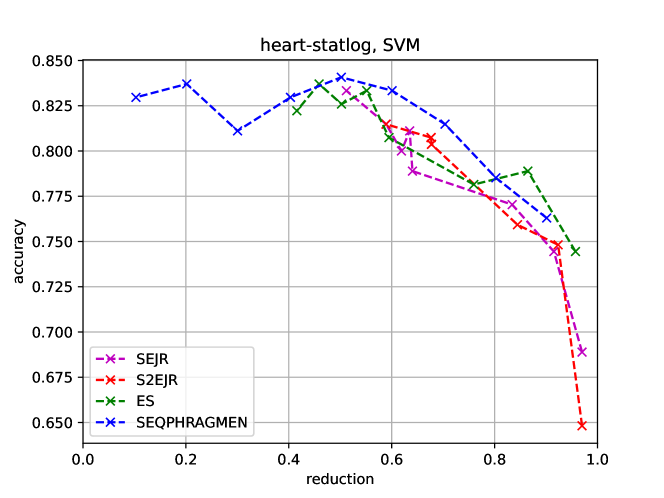
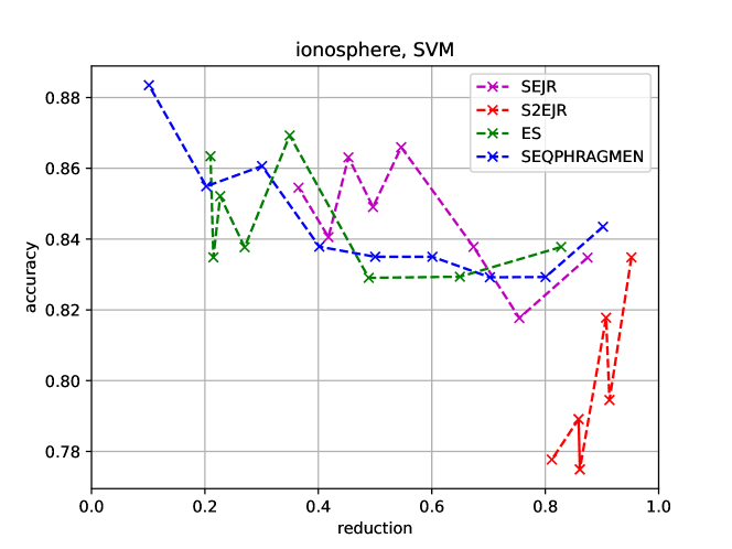
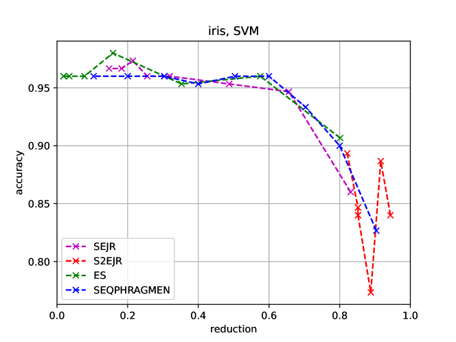
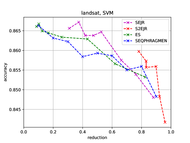
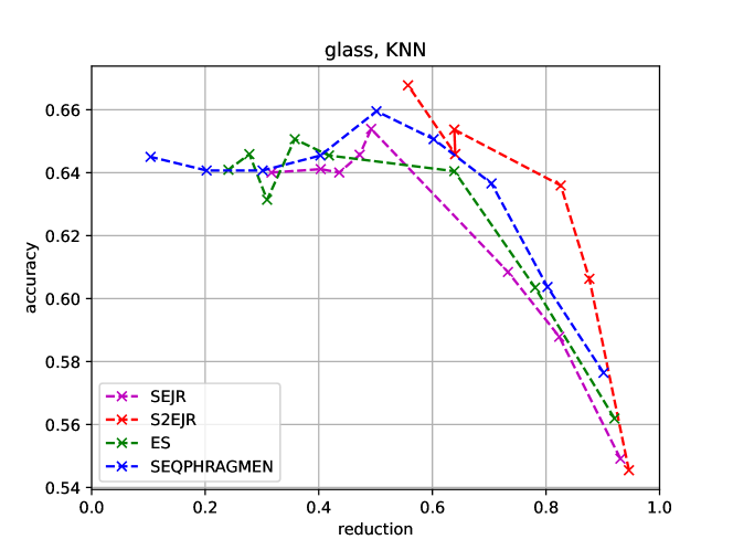
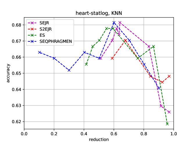
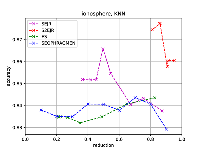
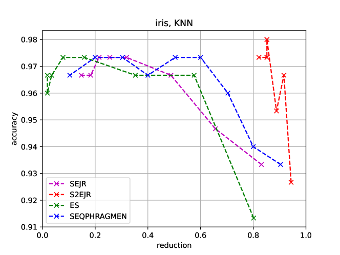
This section contains the accuracy versus reduction figures for each dataset obtained in our experiments. As can be seen in the figures, sometimes an increase in reduction comes also with an increase in accuracy. This phenomenon happens mostly in the smaller datasets and can be also observed in the results for PSDSP reported by [Carbonera and Abel(2018)].

Figure 3: Accuracy vs. reduction plot for the cardiotocography dataset with an SVM classifier

Figure 4: Accuracy vs. reduction plot for the diabetes dataset with an SVM classifier

Figure 5: Accuracy vs. reduction plot for the ecoli dataset with an SVM classifier

Figure 6: Accuracy vs. reduction plot for the glass dataset with an SVM classifier

Figure 7: Accuracy vs. reduction plot for the heart-statlog dataset with an SVM classifier

Figure 8: Accuracy vs. reduction plot for the ionosphere dataset with an SVM classifier

Figure 9: Accuracy vs. reduction plot for the iris dataset with an SVM classifier

Figure 10: Accuracy vs. reduction plot for the landsat dataset with an SVM classifier

Figure 11: Accuracy vs. reduction plot for the letter-recognition dataset with an SVM classifier

Figure 12: Accuracy vs. reduction plot for the optdigits dataset with an SVM classifier

Figure 13: Accuracy vs. reduction plot for the page-blocks dataset with an SVM classifier

Figure 14: Accuracy vs. reduction plot for the parkinson dataset with an SVM classifier

Figure 15: Accuracy vs. reduction plot for the segment dataset with an SVM classifier

Figure 16: Accuracy vs. reduction plot for the spambase dataset with an SVM classifier

Figure 17: Accuracy vs. reduction plot for the wine dataset with an SVM classifier

Figure 18: Accuracy vs. reduction plot for the cardiotocography dataset with a KNN classifier

Figure 19: Accuracy vs. reduction plot for the diabetes dataset with a KNN classifier

Figure 20: Accuracy vs. reduction plot for the ecoli dataset with a KNN classifier

Figure 21: Accuracy vs. reduction plot for the glass dataset with a KNN classifier

Figure 22: Accuracy vs. reduction plot for the heart-statlog dataset with a KNN classifier

Figure 23: Accuracy vs. reduction plot for the ionosphere dataset with a KNN classifier

Figure 24: Accuracy vs. reduction plot for the iris dataset with a KNN classifier

Figure 25: Accuracy vs. reduction plot for the landsat dataset with a KNN classifier

Figure 26: Accuracy vs. reduction plot for the letter-recognition dataset with a KNN classifier

Figure 27: Accuracy vs. reduction plot for the optdigits dataset with a KNN classifier

Figure 28: Accuracy vs. reduction plot for the page-blocks dataset with a KNN classifier

Figure 29: Accuracy vs. reduction plot for the parkinson dataset with a KNN classifier

Figure 30: Accuracy vs. reduction plot for the segment dataset with a KNN classifier

Figure 31: Accuracy vs. reduction plot for the spambase dataset with a KNN classifier

Figure 32: Accuracy vs. reduction plot for the wine dataset with a KNN classifier

References

- [1]
- [Aha et al.(1991)] David W Aha, Dennis Kibler, and Marc K Albert. 1991. Instance-based learning algorithms. Machine learning 6, 1 (1991), 37–66.
- [Aziz et al.(2017)] H. Aziz, M. Brill, V. Conitzer, E. Elkind, R. Freeman, and T. Walsh. 2017. Justified Representation in Approval-Based Committee Voting. Social Choice and Welfare 48 (2017), 461–485.
- [Aziz et al.(2018)] Haris Aziz, Edith Elkind, Shenwei Huang, Martin Lackner, Luis Sánchez-Fernández, and Piotr Skowron. 2018. On the Complexity of Extended and Proportional Justified Representation. In Proceedings of the 32nd Conference on Artificial Intelligence (AAAI-2018). 902–909.
- [Brandt et al.(2016)] Felix Brandt, Vincent Conitzer, Ulle Endriss, Ariel D Procaccia, and Jérôme Lang. 2016. Handbook of computational social choice. Cambridge University Press.
- [Brighton and Mellish(2002)] Henry Brighton and Chris Mellish. 2002. Advances in instance selection for instance-based learning algorithms. Data mining and knowledge discovery 6, 2 (2002), 153–172.
- [Brill et al.(2017)] M. Brill, R. Freeman, S. Janson, and M. Lackner. 2017. Phragmén’s Voting Methods and Justified Representation. In Proceedings of the 31st AAAI Conference on Artificial Intelligence (AAAI-2017). 406–413.
- [Caises et al.(2011)] Yoel Caises, Antonio González, Enrique Leyva, and Raúl Pérez. 2011. Combining instance selection methods based on data characterization: An approach to increase their effectiveness. Information Sciences 181, 20 (2011), 4780–4798.
- [Caragiannis and Fehrs(2022)] Ioannis Caragiannis and Karl Fehrs. 2022. The Complexity of Learning Approval-Based Multiwinner Voting Rules. In Proceedings of the AAAI Conference on Artificial Intelligence, Vol. 36. 4925–4932.
- [Carbonera and Abel(2015)] Joel Luis Carbonera and Mara Abel. 2015. A density-based approach for instance selection. In 2015 IEEE 27th International Conference on Tools with Artificial Intelligence (ICTAI). IEEE, 768–774.
- [Carbonera and Abel(2018)] Joel Luís Carbonera and Mara Abel. 2018. Efficient Instance Selection Based on Spatial Abstraction. In 2018 IEEE 30th International Conference on Tools with Artificial Intelligence (ICTAI). 286–292. https://doi.org/10.1109/ICTAI.2018.00053
- [Conitzer(2010)] V. Conitzer. 2010. Making Decisions Based on the Preferences of Multiple Agents. Commun. ACM 53, 3 (2010), 84–94.
- [Cristianini et al.(2000)] Nello Cristianini, John Shawe-Taylor, et al. 2000. An introduction to support vector machines and other kernel-based learning methods. Cambridge university press.
- [Dua and Graff(2017)] Dheeru Dua and Casey Graff. 2017. UCI Machine Learning Repository. http://archive.ics.uci.edu/ml.
- [Elkind et al.(2017)] Edith Elkind, Piotr Faliszewski, Jean-François Laslier, Piotr Skowron, Arkadii Slinko, and Nimrod Talmon. 2017. What do multiwinner voting rules do? An experiment over the two-dimensional euclidean domain. In Proceedings of the AAAI Conference on Artificial Intelligence, Vol. 31.
- [Faliszewski et al.(2017)] Piotr Faliszewski, Piotr Skowron, Arkadii Slinko, and Nimrod Talmon. 2017. Multiwinner voting: A new challenge for social choice theory. In Trends in computational social choice, Ulle Endriss (Ed.). AI Access, 27–47.
- [García et al.(2015)] Salvador García, Julián Luengo, and Francisco Herrera. 2015. Data preprocessing in data mining. Vol. 72. Springer.
- [Gates(1972)] Geoffrey Gates. 1972. The reduced nearest neighbor rule. IEEE transactions on information theory 18, 3 (1972), 431–433.
- [Hart(1968)] Peter Hart. 1968. The condensed nearest neighbor rule. IEEE transactions on information theory 14, 3 (1968), 515–516.
- [Janson(2016)] S. Janson. 2016. Phragmén’s and Thiele’s election methods. Technical Report. arXiv:1611.08826 [math.HO].
- [Lackner and Skowron(2023)] Martin Lackner and Piotr Skowron. 2023. Multi-Winner Voting with Approval Preferences. Springer Cham.
- [Leyva et al.(2013)] Enrique Leyva, Antonio González, and Raúl Pérez. 2013. Knowledge-based instance selection: A compromise between efficiency and versatility. Knowledge-Based Systems 47 (2013), 65–76.
- [Leyva et al.(2015)] Enrique Leyva, Antonio González, and Raúl Pérez. 2015. Three new instance selection methods based on local sets: A comparative study with several approaches from a bi-objective perspective. Pattern Recognition 48, 4 (2015), 1523–1537.
- [Olvera-López et al.(2010)] J Arturo Olvera-López, J Ariel Carrasco-Ochoa, and J Martínez-Trinidad. 2010. A new fast prototype selection method based on clustering. Pattern Analysis and Applications 13, 2 (2010), 131–141.
- [Peters and Skowron(2020)] Dominik Peters and Piotr Skowron. 2020. Proportionality and the limits of welfarism. In Proceedings of the 21st ACM Conference on Economics and Computation (EC-2020). 793–794.
- [Phragmén(1894)] Edvard Phragmén. 1894. Sur une méthode nouvelle pour réaliser, dans les élections, la représentation proportionelle des partis. Öfversigt af Kongliga Vetenskaps-Akademiens Förhandlingar 51, 3 (1894), 133–137.
- [Pierczynski and Skowron(2019)] Grzegorz Pierczynski and Piotr Skowron. 2019. Approval-based elections and distortion of voting rules. In Proceedings of the 28th International Joint Conference on Artificial Intelligence. 543–549.
- [Procaccia et al.(2009)] Ariel D. Procaccia, Aviv Zohar, Yoni Peleg, and Jeffrey S. Rosenschein. 2009. The learnability of voting rules. Artificial Intelligence 173, 12 (2009), 1133–1149. https://doi.org/10.1016/j.artint.2009.03.003
- [Sánchez-Fernández et al.(2017a)] L. Sánchez-Fernández, E. Elkind, and M. Lackner. 2017a. Committees providing EJR can be computed efficiently. Technical Report. arXiv:1704.00356v3 [cs.GT].
- [Sánchez-Fernández et al.(2017b)] L. Sánchez-Fernández, E. Elkind, M. Lackner, N. Fernández, J. A. Fisteus, P. Basanta Val, and P. Skowron. 2017b. Proportional Justified Representation. In Proceedings of the 31st Conference on Artificial Intelligence (AAAI-2017). 670–676.
- [Wilson(1972)] Dennis L Wilson. 1972. Asymptotic properties of nearest neighbor rules using edited data. IEEE Transactions on Systems, Man, and Cybernetics 3 (1972), 408–421.
- [Wilson and Martinez(2000)] D Randall Wilson and Tony R Martinez. 2000. Reduction techniques for instance-based learning algorithms. Machine learning 38, 3 (2000), 257–286.
- [Zhou(2021)] Zhi-Hua Zhou. 2021. Machine learning. Springer Nature.
Appendix A Results for SEJR
We first prove that SEJR always outputs a committee of size less than or equal to .
Lemma 1.
For any approval-based multi-winner election , the rule SEJR always outputs a committee of size less than or equal to .
Proof.
We divide the operation of SEJR into two parts: (i) iterations in which the maximum plausibility is greater than or equal to for some candidate ; and (ii) iterations in which the maximum plausibility is equal to .