GSpyNetTree: A signal-vs-glitch classifier for gravitational-wave event candidates

Abstract

Despite achieving sensitivities capable of detecting the extremely small amplitude of gravitational waves (GWs), LIGO and Virgo detector data contain frequent bursts of non-Gaussian transient noise, commonly known as ‘glitches’. Glitches come in various time-frequency morphologies, and they are particularly challenging when they mimic the form of real GWs. Given the higher expected event rate in the next observing run (O4), LIGO-Virgo GW event candidate validation will require increased levels of automation. Gravity Spy, a machine learning tool that successfully classified common types of LIGO and Virgo glitches in previous observing runs, has the potential to be restructured as a signal-vs-glitch classifier to accurately distinguish between glitches and GW signals. A signal-vs-glitch classifier used for automation must be robust and compatible with a broad array of background noise, new sources of glitches, and the likely occurrence of overlapping glitches and GWs. We present GSpyNetTree, the Gravity Spy Convolutional Neural Network Decision Tree: a multi-CNN classifier using CNNs in a decision tree sorted via total GW candidate mass tested under these realistic O4-era scenarios.

• April 2023

Keywords: noise, glitch, gravitational-waves, LIGO, Virgo, KAGRA, O4, Gravity Spy, Machine Learning

1 Introduction

Since the first observing run (O1) [1, 2], and following major upgrades [3, 4, 5], the Advanced LIGO (aLIGO) [6] and Advanced Virgo (AdVirgo) [7] detectors have made dozens of transient GW signal detections in the second (O2) [8] and third (O3a, O3b) [9, 10, 11] observing runs. Due to the extreme and increasing sensitivity of these detectors, they are prone to non-astrophysical noise sources (glitches) that can mask or mimic true GW signals [12]. These glitches are particularly problematic as they may generate false-positive candidates [13, 14, 15], corrupt data, and bias astrophysical parameter estimation [16, 17, 18]. Along with the vast amount of data that LIGO and Virgo generate, developing robust tools and methods to automatically identify and characterize these glitches is crucial for extracting GW signals from the data.

A common tool used for glitch classification is Gravity Spy [19, 20]: a Convolutional Neural Network (CNN) image classifier that distinguishes 21 different glitch classes and 1 Chirp class (consisting of data from hardware injections that emulate the behavior of GWs by displacing the detector’s test masses [21]) via time-frequency visualizations, a type of spectrograms called omegascans [22]. A CNN is a type of Deep Learning algorithm designed for image classification consisting of an input layer, an output layer, and several hidden layers that extract useful features from the inputs.

After successfully classifying glitches in previous observing runs [23], Gravity Spy’s architecture has shown the potential to be used as a signal-vs-glitch classifier. This new application is particularly relevant as detectors become more sensitive for the next observing run (O4), and further automation of event candidate validation is required [15].

Numerous investigations using other Machine Learning techniques in glitch classification, such as Principal Component Analysis (PCA) and clustering glitches with Deep Transfer Learning, have been explored [24, 25]. Other approaches also include iDQ, a supervised learning tool that detects detector noise artifacts through auxiliary channel data [26], and GWSkyNet, a low-latency classifier for public GW candidates that requires information from multiple detectors [27]. In order to fully leverage CNNs as the state-of-the-art method for complex image classification tasks [28], we build on Gravity Spy’s CNN classification approach to distinguish signals from glitches for future observing runs using single detector strain $h(t)$ data.

This paper builds upon the proof of principle described in Jarov et al. [29], which outlines a new multi-classifier method to leverage prior Gravity Spy architecture to distinguish GWs from glitches. Considering previous investigations on improving Gravity Spy that have shown that its inaccuracies in glitch classification tend to be higher in poorly represented classes in the CNN’s training set [30], Jarov et al.’s study recommends significant changes to Gravity Spy for the purpose of a signal-vs-glitch classifier. First, it recommends augmenting the data of the Chirp class, which is morphologically similar to the typical GW events seen in O3 [20]. However, instead of using hardware injections, it uses GW software simulations that allow the generation of more GW samples, compared to the severely underrepresented Chirp class in the original Gravity Spy training set [19]. It also recommends deploying specialized training sets to handle different ranges of total candidate signal mass, as low and high-mass mergers have very distinct morphologies, which may be more prone to confusion with particular glitch classes.

We developed this proposed signal-vs-glitch multi-classifier architecture and analyzed its readiness for O4, as described in Section 2. After generating the specialized training sets based on GW and glitch morphology and incorporating the data augmentation suggested by Jarov et al. [29], we built three different classifiers, one per training set, with the same CNN architecture Gravity Spy leverages. With the three signal-vs-glitch classifiers, we made a decision tree sorted via total GW candidate mass, constituting the base for GSpyNetTree, the Gravity Spy Convolutional Neural Network Decision Tree. During O4, this tool will intake GW candidate events from GraceDB [31] and classify them as GWs or glitches as part of the LIGO-Virgo Data Quality Report [32].

After building GSpyNetTree according to the recommendations in Jarov et al. [29], we noted that the original Gravity Spy CNN architecture could be further improved. We decided to use Inception V3 [33], Google’s state-of-the-art CNN for image classification tasks, as explained in section 3. We noted a vast improvement in classification accuracy, particularly for the GW class. We also considered the additional changes expected for O4, including different persistent noise subtraction for calibrated data, new potential noise sources, a high expected detection rate [34], and the likely occurrence of overlapping glitches and GW signals in time-frequency visualizations.

Section 4 presents three validation studies based on the classification challenges posed by the O4 sensitivity increase. Additionally, we propose solutions to overcome them for a future O4-era version of GSpyNetTree. First, we study how the current version of GSpyNetTree responds to data with non-linear subtraction of 60 Hz AC power artifacts, as expected for low latency LIGO data in O4. We evaluate its readiness for the new background noise expected in O4 and its transferability to Virgo data, which has a different noise background from the two LIGO detectors. We also test how GSpyNetTree responds to glitches not included in its training set, as new noise sources are expected to appear during O4. We curate a variety of glitches covering several cases of interest, including frequently occurring glitches and glitches morphologically similar to others already included in the training set. We then evaluate how GSpyNetTree responds to GW candidates overlapping with glitches, which is even more likely to happen during O4 than O3, where 24% of candidates overlapped with one or more glitches [9, 11]. We propose a new multi-label architecture that allows GW classification, even in the case of glitches overlapping with signals. Finally, we comment on prospects for GSpyNetTree in the O4 era.

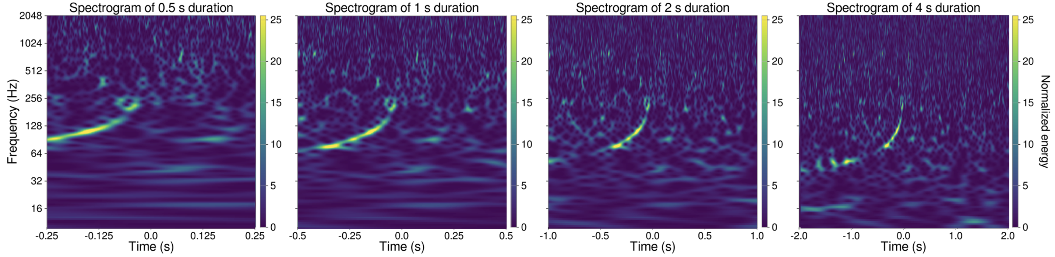
(a)

(b)

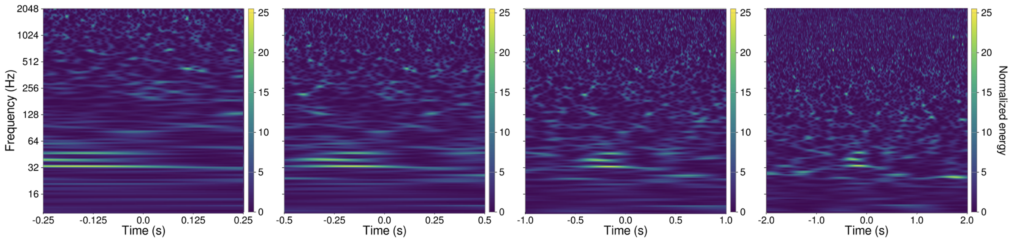
(c)

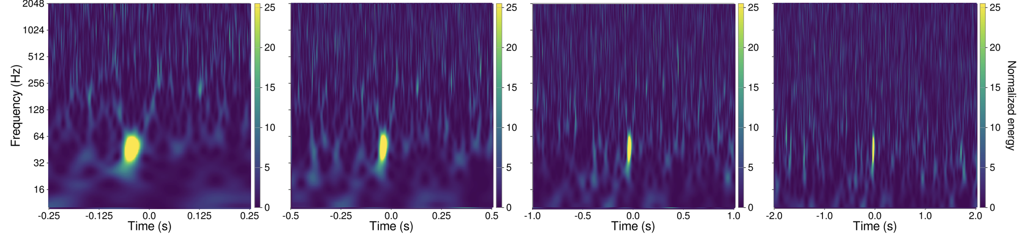
(d)

Figure 1: Examples of spectrograms of simulated GW signals with all four durations used in the training set of GSpyNetTree (0.5 s, 1 s, 2 s, and 4 s). (a) Software simulated GW signal in the low mass regime, with a total mass of 29.2 $M\textsubscript{$\odot$}$. (b) Simulated GW signal in the high mass regime, with a total mass of 118.7 $M\textsubscript{$\odot$}$. (c) Simulated GW signal in the high mass regime, with a total mass of 182 $M\textsubscript{$\odot$}$, but with a significantly lower signal-to-noise ratio (SNR) than the example shown in Figure 1(b). Signals with a low SNR may occur in any of the mass ranges, and they may be similar to the No Glitch class (Figure 2(e)). (d) Simulated GW signal in the extremely high mass regime, with a total mass of 283 $M\textsubscript{$\odot$}$. These signals are morphologically similar to Low-frequency blips (Figure 2(b)).

2 Building GSpyNetTree and its training datasets

Building upon the proof of principle described in Jarov et al. [29], GSpyNetTree leverages a decision tree of three CNN classifiers, each trained on a specialized and balanced set of GWs and morphologically similar glitches, sorted via estimated candidate mass metadata. The three classifiers are: the low-mass (LM) classifier (for candidates with an estimated total mass below 50 M_$\odot$), the high-mass (HM) classifier (for candidates with an estimated total mass between 50 M_$\odot$ and 250 M_$\odot$), and the extremely high-mass (EHM) classifier (for candidates with an estimated total mass above 250 M_$\odot$). Depending on the mass estimate provided via GraceDB [31], each candidate GW event is sent to the LM CNN or HM CNN to determine whether it is astrophysical or a glitch. If the candidate’s mass is above 250 $M\textsubscript{$\odot$}$, it is then sent from the HM classifier to the EHM classifier for more accurate classification. Figure 1 shows examples of simulated GW signals in each of the mass ranges, and Figure 2 shows the glitches they are morphologically similar to. Table 1 specifies the glitch classes considered for each mass range depending on morphological similarities, as considered by Jarov et al. [29].

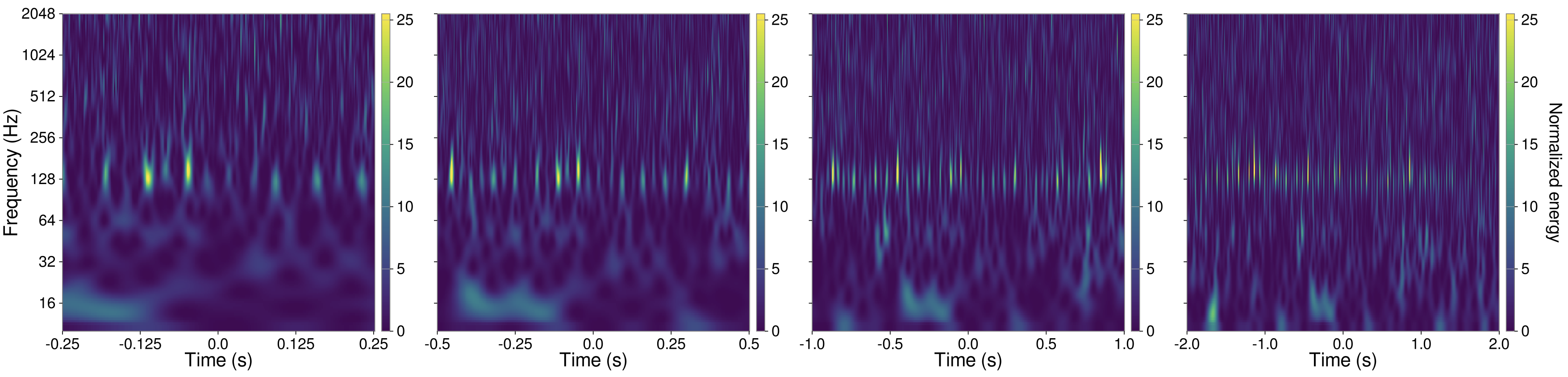
(a) Example of a Scratchy glitch.

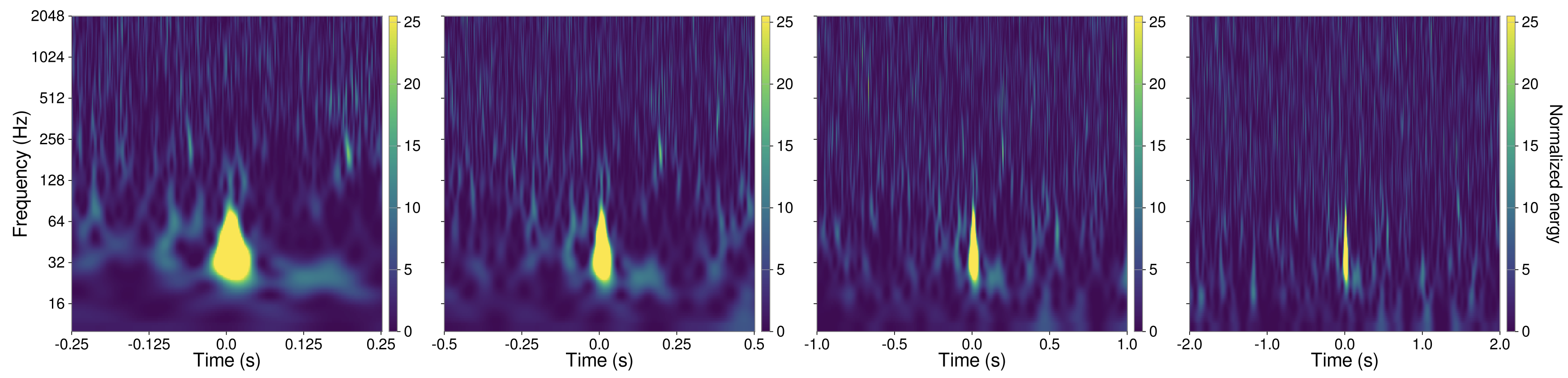
(b) Example of a Low-frequency blip glitch.

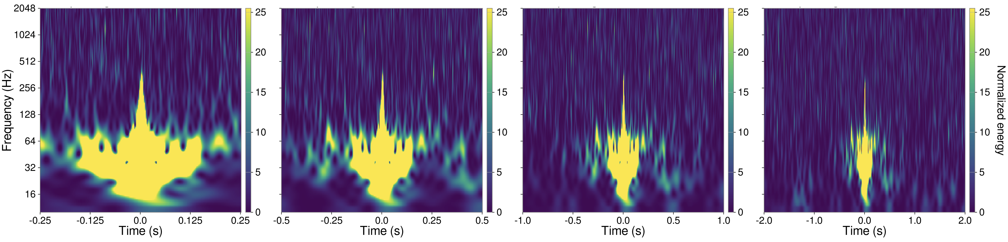
(c) Example of a Koi Fish glitch.

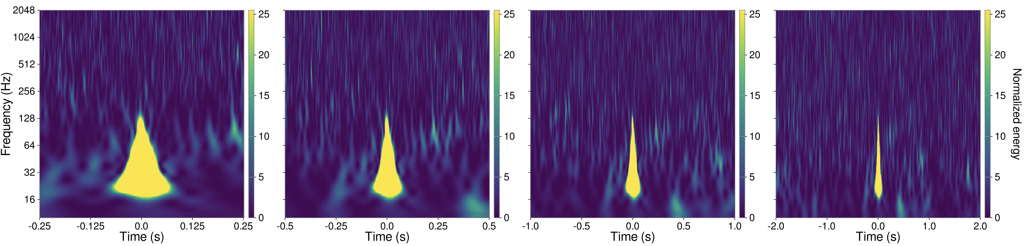
(d) Example of a Tomte glitch.

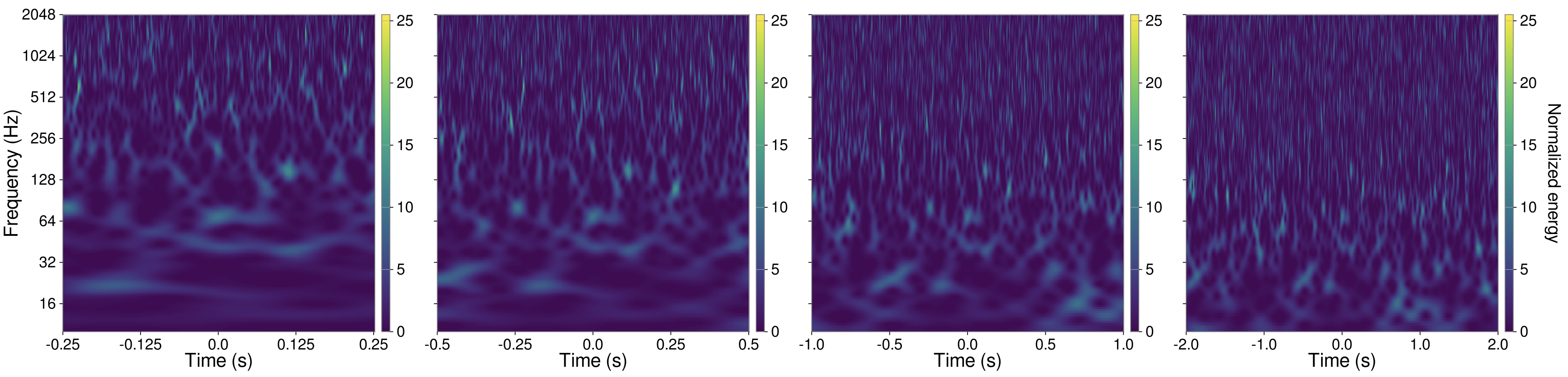
(e) Example of a No Glitch.

Figure 2: Examples of selected glitches with all four durations used in GSpyNetTree (0.5 s, 1 s, 2 s, and 4 s). These non-astrophysical events are morphologically similar to the GW signals in the three mass ranges. All samples fetched from LIGO-DV web [35].

Low-Mass (LM) Classifier		High-Mass (HM) Classifier		Extremely High-Mass (EHM) Classifier
Class	Samples	Class	Samples	Class	Samples
GW (3-50 M$\odot$)	1000	GW (50-250 M$\odot$)	1000	GW (250-350 M$\odot$)	1000
Blip	999	Blip	999	Blip	999
Low-Frequency Blip	1039	Low-Frequency Blip	1039	Low-Frequency Blip	1039
No Glitch	1017	No Glitch	1017	No Glitch	1017
Scratchy	1093	Koi Fish	990
		Tomte	758

Table 1: Classes and number of samples (before time-offset augmentation, which add four more examples for each sample listed) per class for each of the GSpyNetTree’s classifiers. The GW mass ranges listed indicate the target total mass of an event candidate.

The EHM classifier presents additional challenges that need to be addressed. Low-frequency blips share strong similarities in duration, frequency range, and morphology with EHM mergers. Indeed, the original Gravity Spy model misclassifies EHM mergers as Low-frequency blips with 99% confidence [29]. However, since the mass range of detected GWs is expected to increase in each observing run, it is essential to make GSpyNetTree robust for these possible future detections. GSpyNetTree incorporates a spectrogram scaling technique that Jarov et al. showed to be of great utility in this mass range [29]: we apply the Mercator projection, which stretches the signals vertically, scaling the image features to better segregate GW signals from Low-frequency blips.

Additionally, when dealing with CNN training sets, it is important to consider data augmentation techniques to avoid overfitting. One strategy is to generate slightly modified versions of existing samples, increasing the amount of training data. Thus, we generated four random time offsets within $0.1\;\mathrm{s}$ in the time-frequency visualizations of each GW and glitch so that samples are not always perfectly centered. This also makes GSpyNetTree robust to small offsets in estimated candidate merger times.

Following this approach, we built an augmented training set for each of GSpyNetTree’s CNNs. First, we ensured a balanced representation of both GWs and glitches, as previous studies have shown that a higher rate of inaccuracies is related to poorly represented classes in Gravity Spy [30, 29]. Additionally, it is well known for CNN image classifiers that increasing the size of the training set improves classification performance  [36]. Instead of having $\sim 150$ instances per class as in previous studies [29], we decided to enrich our training sets with more samples so that there were $1000\pm 300$ of each per class. Moreover, we included the No Glitch class for the three classifiers to account for GWs with low signal-to-noise ratio (SNR). Table 1 shows the distribution of classes per classifier in the GSpyNetTree training sets.

We fetched all the glitches included in this training set from Gravity Spy classifications via LIGO-DV web [35] for both LIGO Hanford (LHO) and LIGO Livingston (LLO) observatories. Additionally, we manually verified all examples to discard misclassified or morphologically unconventional samples, which we saved for the validation study explained in section 4.2. For the GW simulations, we identified several segments of 64-second quiet detector data for both LHO and LLO during previous observing runs and injected simulated waveforms into them using the inspiral injection module of LALSuite [37], using the waveform model IMRPhenomPv2 [38, 39]. GSpyNetTree’s GW examples are uniformly drawn from a total merger mass range of $5{M\textsubscript{$\odot$}}$ to $350{M\textsubscript{$\odot$}}$, with individual masses ranging from $2{M\textsubscript{$\odot$}}$ to $175{M\textsubscript{$\odot$}}$, an SNR range of 8 to 35, and individual component spins ranging from 0.05 to 0.95.

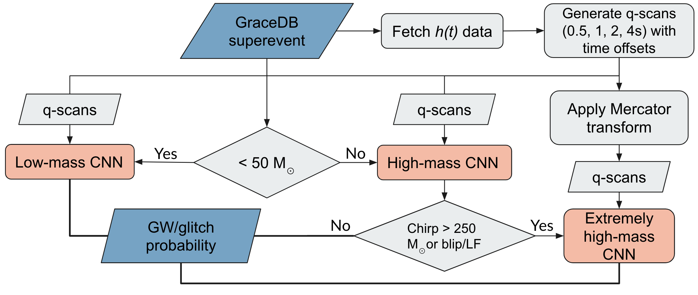
Figure 3: GSpyNetTree architecture: Triggered by a GraceDB superevent [31], time series (strain) data is fetched to generate spectrograms of 0.5, 1, 2, and 4 second durations. Time-frequency spectrogram visualizations are sent to the classifiers based on the estimated candidate merger mass, and the Mercator transform is applied to the extremely high mass GW candidate visualizations. Each CNN outputs the probability that the input visualization contains a GW, an included class of glitch, or no glitch.

We used the strain $h(t)$ time series from each glitch and simulated GW to generate the time-frequency features required by GSpyNetTree for each sample: four spectrograms 0.5 s, 1 s, 2 s, and 4 s in duration arranged in a $2\times 2$ matrix, as in the original Gravity Spy architecture [19]. The different spectrogram durations are used to better capture GW mergers and glitches of different durations. We fed these samples to GSpyNetTree, with architecture shown in Figure 3. After applying the time-offset augmentation, each sample is directed to one of GSpyNetTree’s CNNs, based on its estimated total mass. If the sample’s total mass is less than 50 $M\textsubscript{$\odot$}$, it is directed to the LM classifier; otherwise, it is sent to the HM classifier. Events classified by the HM classifier are further directed to the EHM classifier when the following criteria are met: the total mass of the candidate is estimated to be greater than 250 $M\textsubscript{$\odot$}$ and the HM classifier has classified the candidate as a Low-frequency blip, No Glitch, or GW. In the EHM classifier, the Mercator projection is applied to the sample before classification. Finally, each CNN returns an array of probabilities assigned to each class per sample. Once in production, GSpyNetTree will intake GW candidate events uploaded to GraceDB [31] via the Data Quality Report [32] and classify them as GWs or glitches with a reported probability.

Once GSpyNetTree’s training sets were complete, we trained the CNNs and evaluated their results. We used 80% of the dataset for training, and allocated the remaining 20% for testing the CNNs. Within the training set, we allocated 20% for validation. Section 3 presents these results.

3 A New Architecture for GSpyNetTree

We first tested GSpyNetTree with the augmented training sets described in Section 2, using the original Gravity Spy architecture [19].

Our low-mass CNN had an overall accuracy of 94%, the high-mass CNN achieved 94.6%, while the extremely high-mass CNN made 96% accurate predictions. Additionally, all of them had a 92% accuracy for the GW class, with 7.2%, 4.5%, and 2.9% of GW signals misclassified as No Glitches in the LM, HM, and EHM classifiers, respectively. This was expected for low SNR signals, which may appear faint in spectrogram visualizations. Therefore, these misclassifications are not problematic for GSpyNetTree’s purposes. While these are good results, it is not desirable to misclassify 8% of the astrophysical data per mass range, especially considering the high detection rate expected for O4 [34].

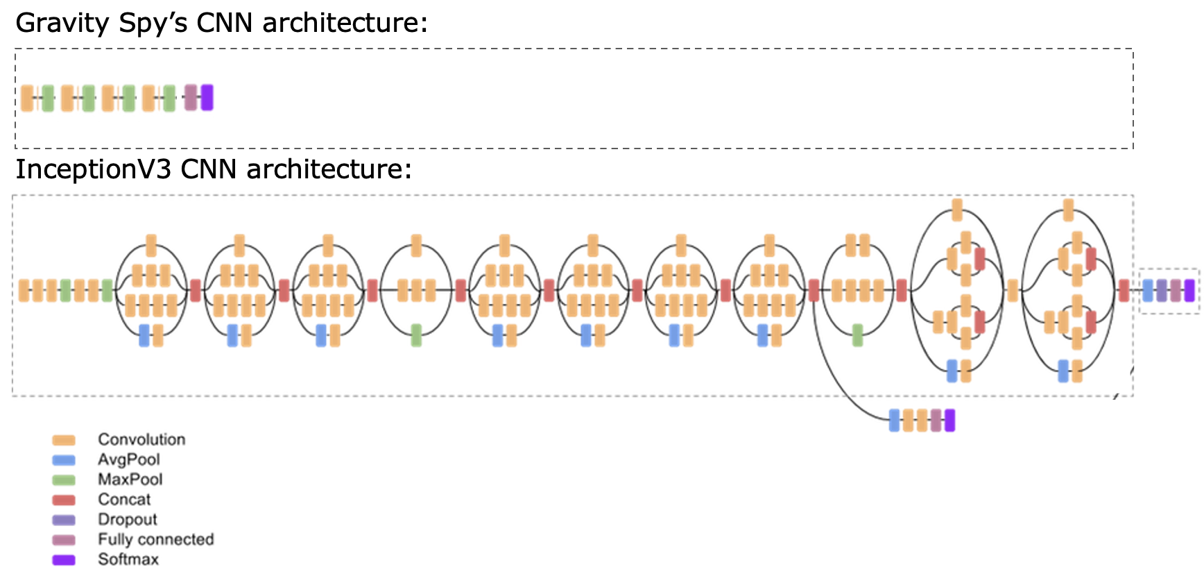
Figure 4: Comparison of the Convolutional Neural Network architecture of Gravity Spy (upper panel) [19] and Inception V3’s architecture (lower panel) [33]. Inception is a more robust, deeper network, which makes it ideal for complex image classification tasks. (Adapted from [33, 40]).

In order to further improve the accuracy of classifications, especially of the GW class, we used a new CNN architecture. It is well known that CNNs are the state-of-the-art method for complex image classification tasks [28]. Therefore, several networks specifically designed to tackle these problems have been studied and developed in the computer science realm. One of them is Inception V3: Google’s state-of-the-art CNN [33]. It is made up of 42 layers, which makes it a very deep model compared to Gravity Spy’s 5 layers, as shown in Figure 4. Additionally, it has shown better accuracy, less computational cost, and a very low error (the percentage of erroneously classified samples) in various image classification tasks. Deeper neural networks require larger training sets to avoid overfitting; however, due to our drastically increased training set size over the one used in Jarov et al. [29], Inception V3 remained a viable option for our investigation.

We trained the three Inception V3 CNNs (LM, HM, and EHM) from scratch, as we had a large enough training set to do so, using the training data introduced in section 2. Figure 5 shows the improvement in classification with this new approach. Following the implementation of the Inception V3 CNNs, all classifiers reached more than 96% accuracy for GWs and all glitch classes, with 3.9%, 2.6%, and 2.3% of GWs misclassified as No Glitches, such that the GW (+ No Glitch) accuracy was 96% (+3.9%), 96% (+2.6%), and 97% (+2.3%) for the LM, HM, and EHM classifiers. This is a considerable decrease in the amount of misclassified astrophysical events.

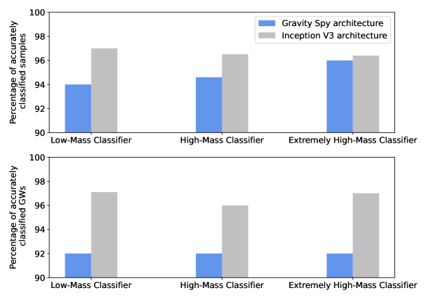
Figure 5: Accuracy results for the three GSpyNetTree CNNs trained using the Gravity Spy architecture (in blue) and the InceptionV3 architecture (in gray) for all GWs and glitches in the test set (upper panel) and for only GWs (lower panel). In the case of chirps, the classification accuracy improved from 92% in all three cases to 97% (LM), 96% (HM), and 97% (EHM). Additionally, overall accuracy also improved from 94%, 95%, and 96% to 97%, for the LM, HM, and EHM classifiers respectively.

Once we improved the classification accuracy of GW signals, we validated GSpyNetTree’s readiness for O4 by performing three validation studies. We tested both the original Gravity Spy and the Inception V3 architecture, and our results were better with the latter for all validation studies. We present these results in Section 4.

4 Validating GSpyNetTree’s readiness for O4

4.1 Testing the CNNs reliance on background

The first validation study we performed aimed to evaluate the dependence of GSpyNetTree on detector background noise. This is important for O4 because the noise subtraction used to produce low-latency calibrated $h(t)$ is expected to differ from previous observing runs. O4 low-latency data is expected to use a non-linear subtraction of AC 60 Hz power artifacts, similar to the technique used for publically released data from the O3 run [41]. It is also important to evaluate how transferable the GSpyNetTree model is to detect GWs for Virgo and KAGRA detectors, which have a different noise background from LIGO.

To test the CNNs’ reliance on background, we used 100 glitch examples per glitch class, using the non-linear 60 Hz subtracted strain channel, for each classifier. Figure 6 shows an example of a Blip fetched from the original (left) and the clean (right) channels.

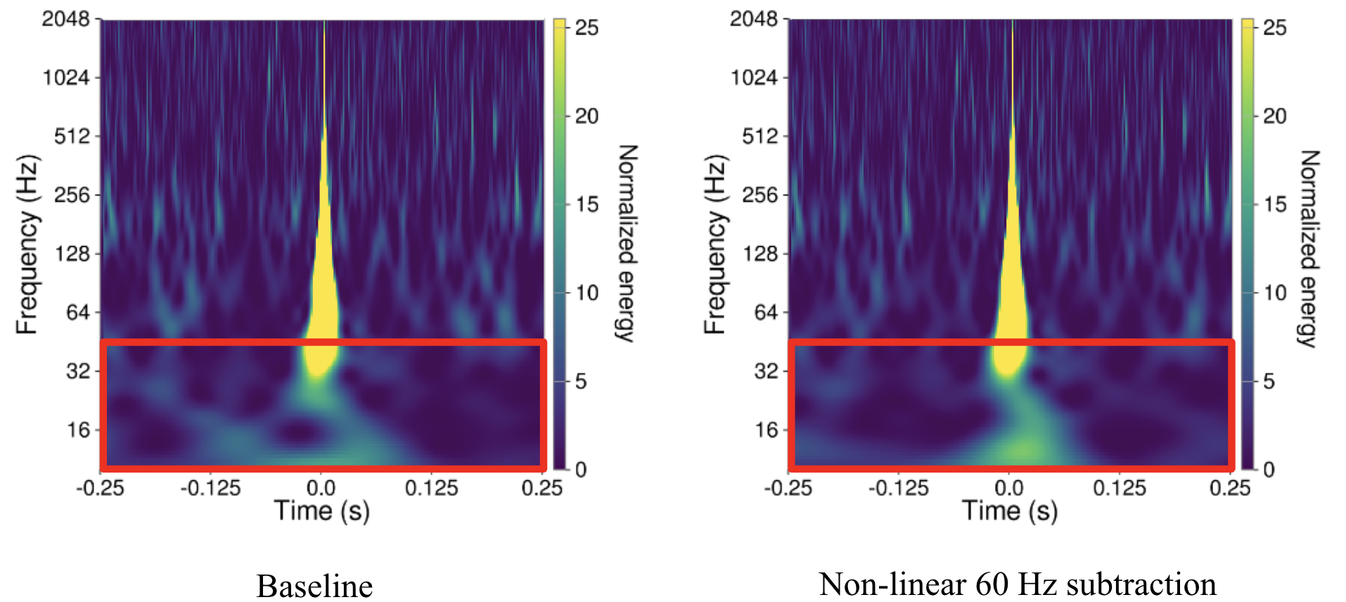
Figure 6: Spectrograms of an O3-era Blip from the Hanford detector, fetched from the original low-latency strain channel (left) and the higher-latency channel with a non-linear subtraction applied (right). A subtle difference in background can be seen around 60 Hz, as shown in the red boxes. The non-linear subtraction is expected to be implemented for low-latency data in O4.

Even though both spectrograms look quite similar to the naked eye, these small differences in background significantly impact CNN accuracy. In fact, when tested with non-linearly noise subtracted data, overall accuracy decreased to 76%, 75%, and 76% for the LM, HM, and EHM classifiers, respectively. Additionally, as shown in Figure 7, individual class accuracy also decreased for all of the glitches but one (Koi Fish). This likely occurs because, as shown in Figure 2(c), these glitches usually cover a wide frequency and time range, so the denoised background data does not significantly impact the visualization.

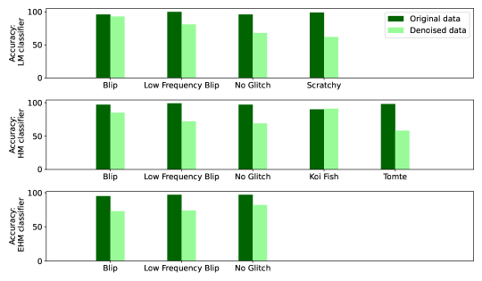
Figure 7: Accuracy results for the LM (top), HM (middle), and EHM (bottom) classifiers for each of the glitches in the validation set. Except for Koi Fish glitches, there is a significant decrease ($\sim 20\%$) in accuracy when denoised background data is used.

Following this discovery, we note that to be able to transfer GSpyNetTree to O4 with maximum accuracy, the CNN’s dependence on background should be addressed with a new augmented training set. Additionally, as only LHO and LLO glitches and background are currently used, we should include Virgo GWs and glitches in our training sets for the O4-era GSpyNetTree. This way, the glitch dataset will be robust enough to account for changes in detector background noise.

4.2 Testing CNN classification of glitches not included in the original training set

Our second validation study focused on studying the CNNs’ performance for glitches not included in the original training set, which was restricted to avoid excess glitch classes that could reduce CNN performance. We selected 8 samples of thunder glitches, all of which occurred during O3, and more than 100 samples of Scattering, Extremely Loud, and Repeating Blips glitches from previous observing runs. An example of each is shown in Figure 8. While the former type of glitch is not a Gravity Spy class, the three latter are part of the Gravity Spy training set.

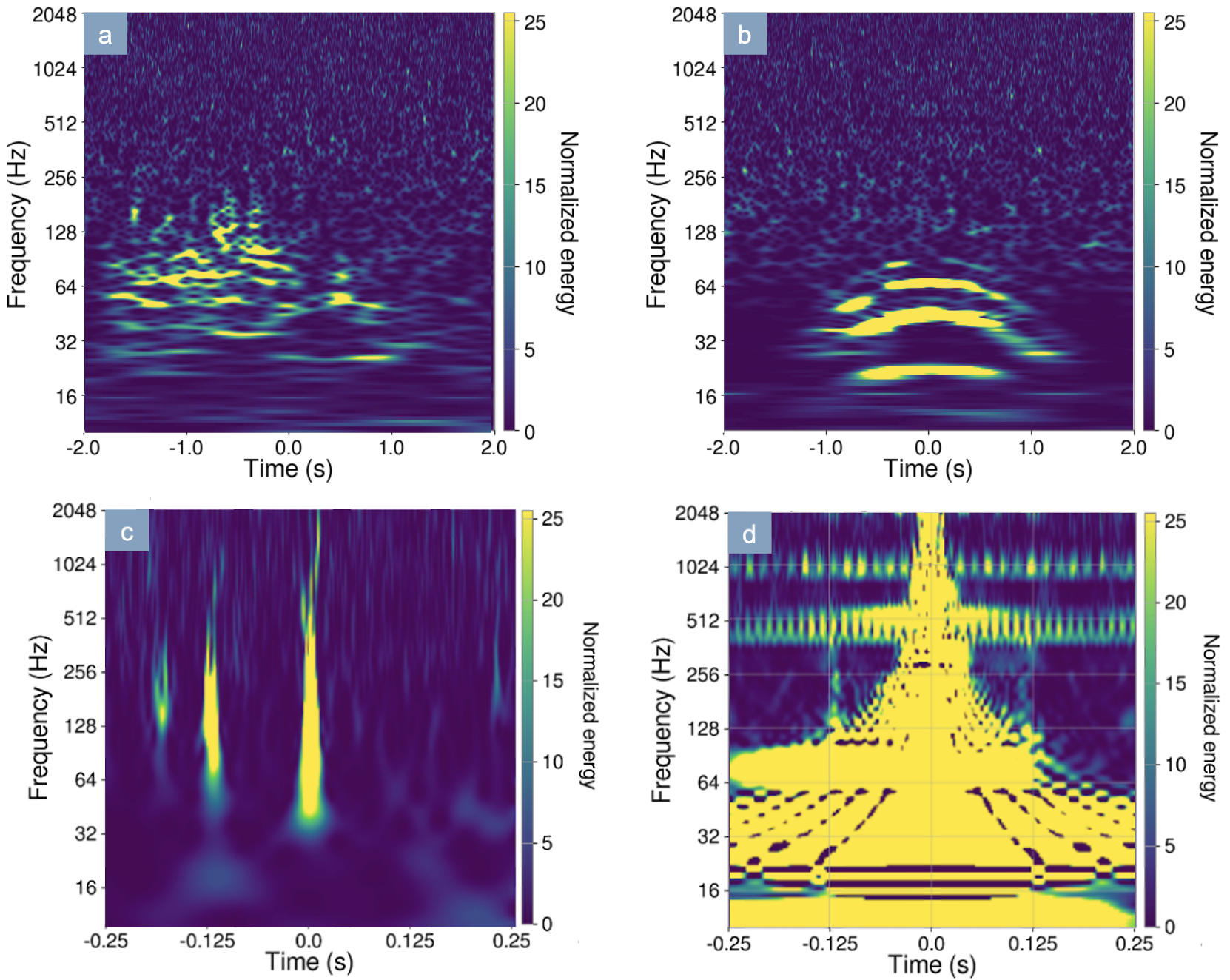
Figure 8: Examples of the glitches used for the validation study that tests glitches not included in the original GSpyNetTree training sets: (a) thunder glitch, (b) Scattering glitch, (c) Repeating Blips, and (d) Extremely Loud glitch. The Thunder and Scattering glitches are shown in a different time scale than the other glitches to highlight their morphology and duration.

We selected each type of glitch to address possible classification challenges that may arise with GSpyNetTree during O4. Scattering and thunder glitches are fairly common [14], so it is more likely that they may appear at the same time as a candidate GW. Repeating Blips were an interesting case because we already had both Blips and Low-frequency blips in the training sets of the three classifiers. Studying the CNNs’ performance in cases where these glitches repeated in the spectrograms allowed us to preliminarily study how the CNN performed with multiple glitches in the same visualization. Extremely loud glitches are morphologically similar to Koi Fish glitches: they both extend in a wide frequency and time range. Thus, including them in our validation study allowed us to evaluate the CNNs performance on morphologically similar glitches.

We tested the three GSpyNetTree classifiers using all the examples considered for this validation study. The classification results for the LM, HM, and EHM classifiers are shown in Figures 9(a), 9(c), and 9(b), respectively. First, it is important to highlight that several glitches are often classified as GWs. A lack of robustness to glitches not included in the training set could be particularly problematic in O4, as new noise sources may appear (with the increase in the detectors’ sensitivity).

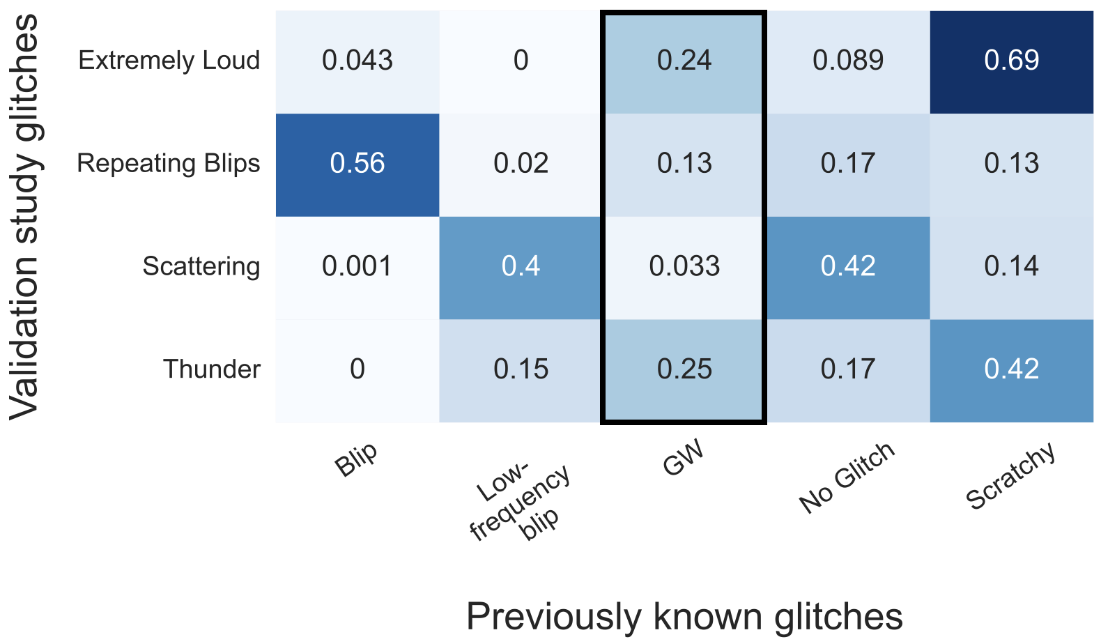
(a) Confusion matrix for the LM classifier of GSpyNetTree for glitches not included in the original training set.

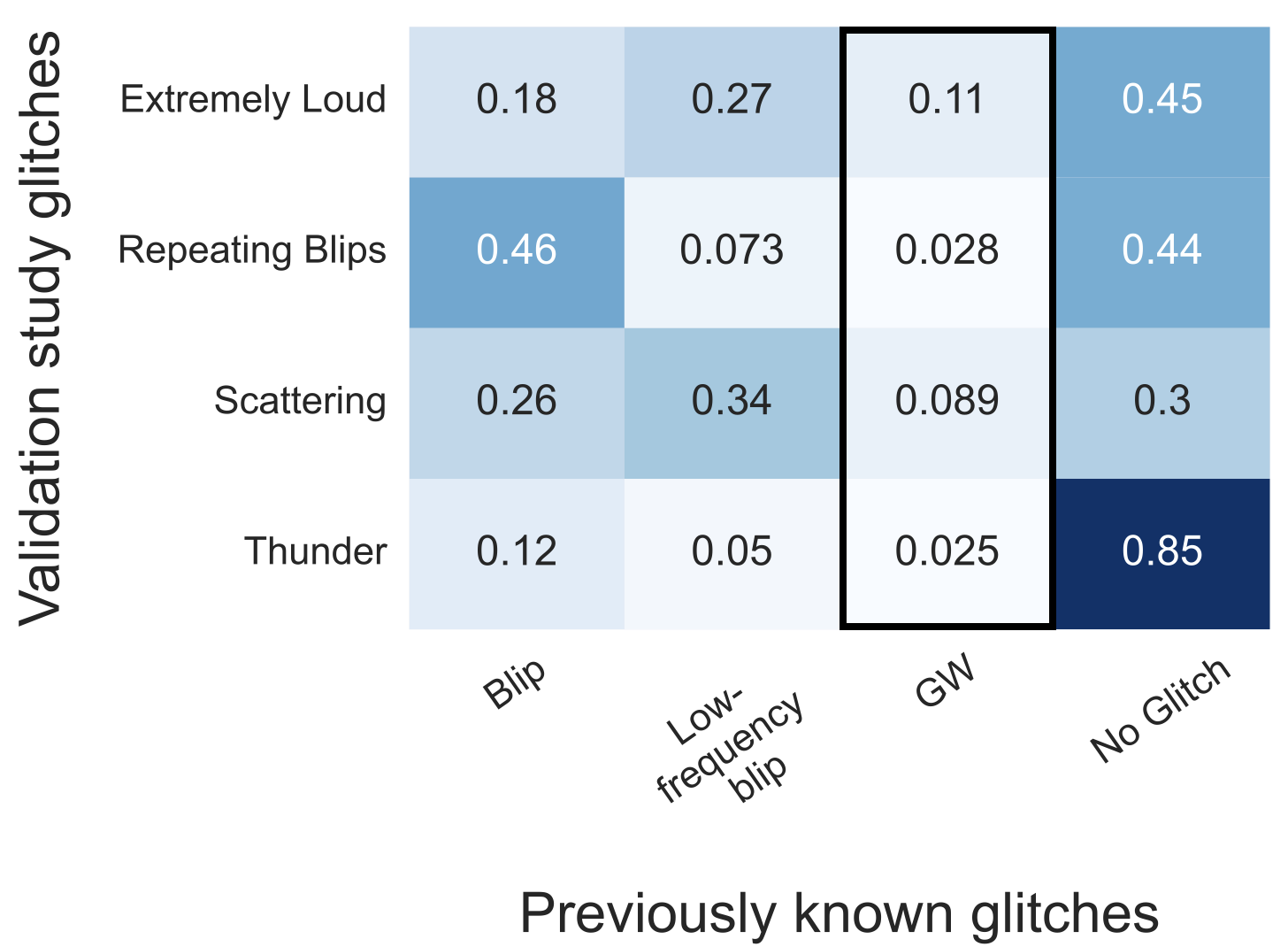
(b) Confusion matrix for the EHM classifier of GSpyNetTree for glitches not included in the original training set.

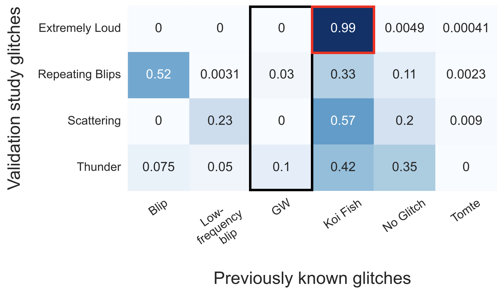
(c) Confusion matrix for the HM classifier of GSpyNetTree for glitches not included in the original training set.

Figure 9: Confusion matrices for the (a) LM, (b) EHM, and (c) HM classifiers in the testing set for the validation study of glitches not included in the original training set: Scattering, Repeating Blips, Thunder, and Extremely Loud glitches. The x and y axes represent the predicted and true classes, respectively, and the confusion matrices are normalized by the total number of glitches of each class of the validation set. The black boxes highlight the fraction of glitches misclassified as GWs. The red box in the confusion matrix of the HM classifier highlights the fraction of Koi Fish glitches misclassified as Extremely Loud glitches.

Overall, this validation study shows that the CNNs have low confidence when classifying new glitches. The classification probability is almost evenly distributed among all classes (including GWs) for most of the glitches in the three classifiers. This is, however, not the case for Repeating Blips and Scattering (in all three CNNs), and Extremely Loud glitches (in the HM classifier). Repeating Blips were classified as Blips with 56%, 52%, and 46% accuracy for the LM, HM, and EHM classifiers, respectively. Even though these results can be further improved, this is promising evidence that the CNN architecture can be tuned to better classify repeating glitches.

Scattering glitches have significantly different behavior in the three classifiers. In the LM CNN, they are mistaken for No Glitches (42%) and Low-frequency blips (40%), possibly because they evolve in a low-frequency range. However, the probability is distributed among the three non-GW classes in the EHM classifier. On the other hand, the HM CNN classifies most of the Scattering glitches (57%) as Koi Fish glitches, suggesting that it focuses on the broad (low)-frequency range the Scattering glitches cover. Since Scattering glitches are one of the most common glitches in current GW detectors and having shown such different behavior among the three CNNs, this is strong evidence that this glitch class should be included as part of the O4-era GSpyNetTree training set.

Moreover, morphologically similar glitches (particularly Koi Fish and Extremely Loud glitches, which both display saturated spectrograms) were classified with 99% accuracy as the class already known by the HM CNN, as shown in the red box in Figure 9(c), and they are not easily mistaken for GWs. This is desirable as GSpyNetTree should minimize flagging non-astrophysical glitches as GW candidates. Even though not as morphologically similar as Koi Fish glitches, the LM CNN classified Extremely Loud glitches as the most dispersed in time and frequency glitch it knows: the Scratchy glitch. However, as opposed to the HM CNN, it misclassifies 24% of them as GWs, which is undesirable if we intend to mitigate the false positive rate. On the other hand, the EHM classifier has a peculiar behavior when classifying both thunder and Extremely Loud glitches. As shown in Figure 9(b), 85% and 45% of the samples are misclassified, respectively, as No Glitches. Covering a wide time-frequency range with a high SNR, it is counter-intuitive that they are both classified in the No Glitch class.

In light of this behavior, an option to address misclassifications of new glitches is creating a new class for unknown or miscellaneous noise sources. However, this may reduce both the overall and GW classification accuracy, as we would be including glitches with substantially different morphologies in the same class, and it does not allow us to investigate new noise sources. Although the easiest solution is to include as many new classes in the CNNs as glitches arise, this approach will potentially reduce the performance of the CNN (as it has more classes it can get confused with).

To solve this issue for the O4-era GSpyNetTree, we propose to use each CNN as a feature extractor in a semi/unsupervised learning task, similar to the approach followed by George et al. [25]. This way, each CNN’s last layer would be projected to a 3-dimensional space using the T-distributed Stochastic Neighborhood Embedding (t-SNE) algorithm [42], such that glitches form clusters whose positions in the 3-d space depend on their morphology. Outliers (glitches not included in the original training set) may create a new cluster (i.e., a new glitch class) or may be separated enough to be segregated from training set classes for further detector characterization and glitch mitigation studies. Compared to the other alternatives, this approach would successfully distinguish new glitch classes from GWs, which is desirable for the O4-era GSpyNetTree signal-vs-glitch classifiers to maximize the detection of astrophysical events with a low false alarm rate.

4.3 Testing overlapping glitches and GWs

As the aLIGO and AdVirgo detectors become more sensitive and the rate of detected events increases, the probability of overlapping glitches and GW signals in strain data also rises. This is a very likely scenario in O4, as it already happened with 26% and 23% of the candidates during the first [9] and second [11] parts of O3. Thus, we tested GSpyNetTree’s performance in cases in which candidates occur in a similar time window as glitches to investigate whether this hinders the classification of true GWs.

To test GSpyNetTree’s ability to accurately classify GWs in the presence of glitches, we generated 30 events per glitch class, for each of the classifiers. First, we injected 3 GWs with different astrophysical parameters (but in the same parameter space as in training) into one of the glitches already learnt in training by the classifier. We then generated 10 normally distributed offsets ($\mu=0\;,\sigma=0.25\;\mathrm{s}$) so that the glitch was shifted in time with respect to the GW signal. This way, we could test GW signals (with different SNR, mass, and spin of the mergers) with offset glitches occurring in the same time window of each spectrogram. An example of a high mass GW and a Tomte glitch can be seen in Figure 10.

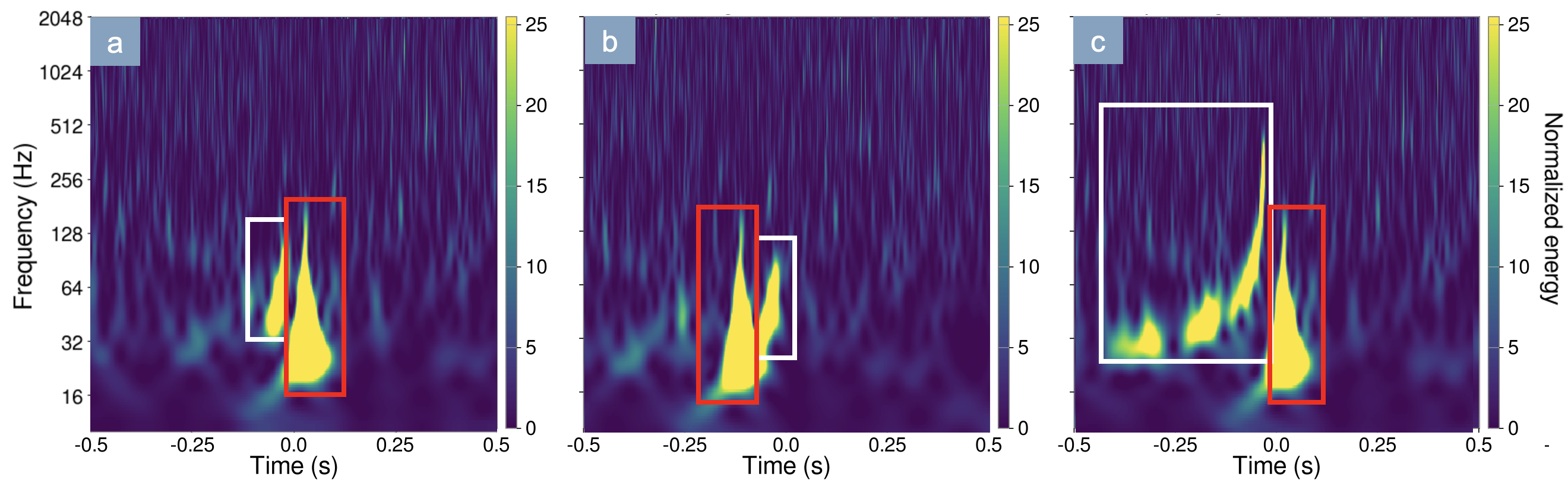
Figure 10: Samples of GWs (white boxes) injected in close proximity to Tomte glitches (red boxes). (a) and (b) show the same GW (with a total mass of 191.8 $M\textsubscript{$\odot$}$), but the glitch has a different time-offset with respect to the GW: $0.011$ s and $-0.130$ s, respectively. (c) shows the Tomte glitch with the same time offset as in (a), but the GW signal has different astrophysical parameters (a total mass of 52 $M\textsubscript{$\odot$}$).

Figure 11 shows the results of this validation study for the three classifiers. More than 60% of the GW signals in the presence of glitches are misclassified as glitches (70% for the HM classifier). Whenever not flagged as GWs, the LM and HM CNNs classified the overlapping GW and glitch events as the longest duration or most saturated glitches they were exposed to during training: Scratchy glitches and Blips in the LM classifier and Koi Fish and Tomte glitches in the HM classifier, as shown in Figure 11.

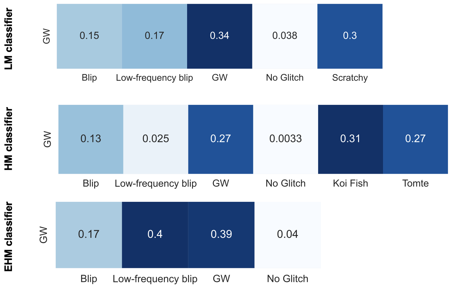
Figure 11: Accuracy results for the LM (top), HM (middle), and EHM (bottom) classifiers for the overlapping gravitational-waves and signals in the validation study. More than 60% (70% for the HM classifier) of the samples are misclassified as glitches.

The EHM classifier tends to inaccurately classify overlapping GWs and glitches as Low-frequency blips, with almost the same probability (40%) as it classifies them as GWs (39%). In all three CNNs, having such a high fraction of candidates flagged as glitches may result in unnecessarily vetoed candidates, an issue that must be avoided for O4. It is clear that GSpyNetTree’s robustness to these events must be increased for it to be used as an element of fully-automated validation of LIGO-Virgo event candidates.

We expect GSpyNetTree misclassifies most of the overlapping glitch and GW events because it is a multi-class classifier: it outputs the probability that a given sample belongs to one particular class, which is independent and mutually exclusive with the other classes. This justifies exploring a multi-label classifier, which would support the prediction of multiple mutually non-exclusive classes, also called labels [43]. This way, the GW signal (or, equivalently, the Tomte glitch) will not be ignored by the classifier, but both of them will be correctly classified as the classes they belong to, as shown in Figure 12.

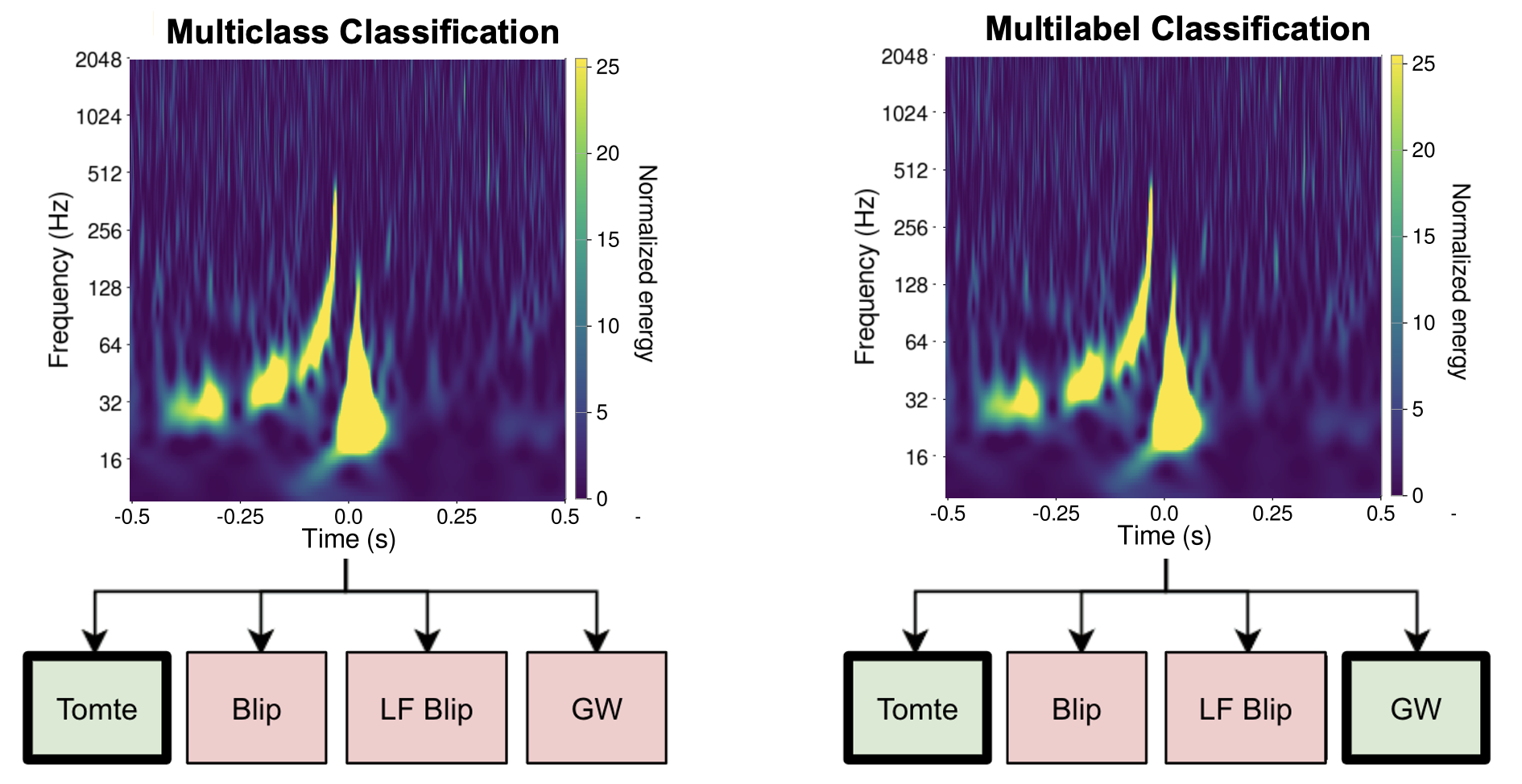
Figure 12: Differences between a multi-class (left) and a multi-label (right) classifier. In the first case, the CNN is only able to identify one of the mutually exclusive classes it was trained on (making it prone to misclassify astrophysical data as glitches). In this particular example, the classifier only detects the Tomte glitch from a sample with an overlapping GW signal. The multi-label architecture would solve this issue. Being able to output several classes from a single sample, both the GW signal and the Tomte glitch would be accurately classified.

We expect that a multi-label classifier will also be able to accurately classify instances of overlapping glitches (such as the Repeating Blips, explained in section 4.2 and shown in Figure 8), without including them as a separate class during training. As GW detector data contains a high rate of glitches, glitches of different types and morphologies often overlap, and we expect that a future multi-label architecture of GSpyNetTree would also be able to accurately classify candidate events associated with overlapping glitches.

5 Conclusions

Based on the proof of principle introduced in Jarov et al. [29] and building on the success of Gravity Spy [19], we built GSpyNetTree, a multi-CNN decision tree of signal-vs-glitch classifiers. We leverage three CNNs, initially based on the original Gravity Spy architecture [19], each of which is trained with specialized training sets, depending on the mass of simulated GW mergers and morphologically similar glitches. We consider three total mass ranges: 3-50 M_$\odot$, 50-250 M_$\odot$, and 250-350 M_$\odot$  for low, high, and extremely-high mass GWs, respectively.

After achieving a 92% accuracy for the GW class in the three CNNs, we noticed that we could use another architecture to further increase the amount of accurately classified samples. We implemented Inception V3, Google’s state-of-the-art CNN for image classification tasks, and achieved more than 96% accuracy for all classifiers.

With better classification results, we tested GSpyNetTree for the O4-era detector’s sensitivity, aiming to have all the signal-vs-glitch classifiers robust to a wide variety of background noise, new sources of glitches, and the likely occurrence of overlapping glitches and GWs. To test the CNNs’ reliance on background, we evaluated GSpyNetTree’s performance on the same types of glitches as in training, but this time using data with non-linear subtraction of 60 Hz AC power artifacts, as expected in O4. We discovered that the classification accuracy decreased to less than 77% for the three classifiers, suggesting that even small changes in background noise significantly impact classification. For future work, we suggest creating a new training set that includes the original glitches and the glitches with the non-linear subtraction, as well as Virgo glitches and GWs, to mitigate dependence on background noise for the O4-era GSpyNetTree.

We also tested GSpyNetTree’s performance on glitches not included in the original training set: Scattering, Thunder, Repeating Blips, and Extremely Loud glitches. We noted that many non-astrophysical events were flagged as GW candidates, which is undesirable as we want to limit the false positive rate. Although the classification results varied considerably among the three CNNs, it was clear that very common glitches that are more likely to appear at the same time as a GW candidate (such as Scattering) should be included in GSpyNetTree’s O4 training set. We observed that glitches morphologically similar to a training glitch class were confidently predicted as that class. Following George et al. [25], we propose to add an unsupervised learning step that uses the CNNs as feature extractors projected into a 3-dimensional space, such that glitches form clusters where position depends on their morphology. New glitches with different morphologies might be segregated enough in that 3-d space from the original classes (especially true GWs), avoiding the need to increase the number of training classes used in the CNNs.

The last validation study we conducted evaluated GSpyNetTree’s current capabilities in the likely case of overlapping GW signals and glitches during O4. We noticed that, for the three CNNs, more than 60% of the astrophysical events with glitches nearby in time were classified as glitches. This is undesirable for O4, as we want to avoid misclassifying GW candidates. To address this, we propose future efforts implement a multi-label architecture replacing the current classifiers. This would allow glitches and GW signals appearing in close proximity to be simultaneously and correctly classified.

In summary, we suggest that the O4-era GSpyNetTree consist of three Inception V3 multi-label classifiers, each trained on a specialized training set including GWs in the three total mass ranges previously studied, along with morphologically similar glitches. These training sets should incorporate data augmentation, apply the Mercator transform to EHM samples, and include LIGO glitches of previous observing runs, as well as examples with a non-linear subtraction of AC 60 Hz power artifacts and Virgo glitches, to account for different backgrounds. Lastly, we suggest using the CNNs as feature extractors to detect and cluster new glitch classes, as well as known glitch classes not included in the GSpyNetTree training set.

6 Acknowledgements

This material is based upon work supported by NSF’s LIGO Laboratory which is a major facility fully funded by the National Science Foundation. We would like to acknowledge and thank the Detector Characterization team of the LSC for their comments and suggestions, particularly to Beverly Berger, Derek Davis, Seraphim Jarov, and Siddharth Soni for very useful discussions. We also thank ManLeong (Mervyn) Chan for his continuous technical support during this project. The authors are grateful for computational resources provided by the LIGO Laboratory and supported by National Science Foundation Grants PHY-0757058 and PHY-0823459. SA is supported by the Mitacs Globalink Research Internship, AL and JD by the NSERC USRA award, and JM by the Canada Research Chairs program.

References

- [1] B.. Abbott et al. “Observation of Gravitational Waves from a Binary Black Hole Merger” In Phys. Rev. Lett. 116 American Physical Society, 2016, pp. 061102 DOI: 10.1103/PhysRevLett.116.061102
- [2] B.. Abbott et al. “GW150914: The Advanced LIGO Detectors in the Era of First Discoveries” In Phys. Rev. Lett. 116 American Physical Society, 2016, pp. 131103 DOI: 10.1103/PhysRevLett.116.131103
- [3] B.. Abbott et al. “Calibration of the Advanced LIGO detectors for the discovery of the binary black-hole merger GW150914” In Phys. Rev. D 95 American Physical Society, 2017, pp. 062003 DOI: 10.1103/PhysRevD.95.062003
- [4] J.. Driggers et al. “Improving astrophysical parameter estimation via offline noise subtraction for Advanced LIGO” In Phys. Rev. D 99 American Physical Society, 2019, pp. 042001 DOI: 10.1103/PhysRevD.99.042001
- [5] A. Buikema et al. “Sensitivity and performance of the Advanced LIGO detectors in the third observing run” In Phys. Rev. D 102 American Physical Society, 2020, pp. 062003 DOI: 10.1103/PhysRevD.102.062003
- [6] LIGO Scientific Collaboration et al. “Advanced LIGO” In Classical and Quantum Gravity 32.7, 2015, pp. 074001 DOI: 10.1088/0264-9381/32/7/074001
- [7] F. Acernese et al. “Advanced Virgo: a second-generation interferometric gravitational wave detector” In Classical and Quantum Gravity 32.2, 2015, pp. 024001 DOI: 10.1088/0264-9381/32/2/024001
- [8] B.. Abbott et al. “GWTC-1: A Gravitational-Wave Transient Catalog of Compact Binary Mergers Observed by LIGO and Virgo during the First and Second Observing Runs” DOI: 10.1103/PhysRevX.9.031040
- [9] B.. Abbott et al. “GWTC-2: Compact Binary Coalescences Observed by LIGO and Virgo During the First Half of the Third Observing Run” DOI: 10.1103/PhysRevX.11.021053
- [10] The LIGO Scientific Collaboration et al. “GWTC-2.1: Deep Extended Catalog of Compact Binary Coalescences Observed by LIGO and Virgo During the First Half of the Third Observing Run” arXiv, 2021 DOI: 10.48550/arXiv.2108.01045
- [11] B.. Abbott et al. “GWTC-3: Compact Binary Coalescences Observed by LIGO and Virgo During the Second Part of the Third Observing Run” DOI: 10.48550/arXiv.2111.03606
- [12] B P Abbott et al. “Characterization of transient noise in Advanced LIGO relevant to gravitational wave signal GW150914” In Classical and Quantum Gravity 33.13 IOP Publishing, 2016, pp. 134001 DOI: 10.1088/0264-9381/33/13/134001
- [13] B.. Abbott et al. “Effects of data quality vetoes on a search for compact binary coalescences in Advanced LIGO’s first observing run” In Classical and Quantum Gravity 35.6, 2018, pp. 065010 DOI: 10.1088/1361-6382/aaaafa
- [14] D Davis et al. “LIGO detector characterization in the second and third observing runs” In Classical and Quantum Gravity 38.13 IOP Publishing, 2021, pp. 135014 DOI: 10.1088/1361-6382/abfd85
- [15] D Davis et al. “Subtracting glitches from gravitational-wave detector data during the third LIGO-Virgo observing run” In Classical and Quantum Gravity 39.24 IOP Publishing, 2022, pp. 245013 DOI: 10.1088/1361-6382/aca238
- [16] Jade Powell “Parameter estimation and model selection of gravitational wave signals contaminated by transient detector noise glitches” In Classical and Quantum Gravity 35.15 IOP Publishing, 2018, pp. 155017 DOI: 10.1088/1361-6382/aacf18
- [17] Ronaldas Macas et al. “Impact of noise transients on low latency gravitational-wave event localization” In Phys. Rev. D 105 American Physical Society, 2022, pp. 103021 DOI: 10.1103/PhysRevD.105.103021
- [18] Ethan Payne et al. “Curious case of GW200129: Interplay between spin-precession inference and data-quality issues” In Phys. Rev. D 106 American Physical Society, 2022, pp. 104017 DOI: 10.1103/PhysRevD.106.104017
- [19] M Zevin et al. “Gravity Spy: integrating advanced LIGO detector characterization, machine learning, and citizen science” In Classical and Quantum Gravity 34.6 IOP Publishing, 2017, pp. 064003 DOI: 10.1088/1361-6382/aa5cea
- [20] S Soni et al. “Discovering features in gravitational-wave data through detector characterization, citizen science, and machine learning” In Classical and Quantum Gravity 38.19 IOP Publishing, 2021, pp. 195016 DOI: 10.1088/1361-6382/ac1ccb
- [21] C. Biwer et al. “Validating gravitational-wave detections: The Advanced LIGO hardware injection system” In Physical Review D 95.6 American Physical Society (APS), 2017 DOI: 10.1103/physrevd.95.062002
- [22] S Chatterji, L Blackburn, G Martin and E Katsavounidis “Multiresolution techniques for the detection of gravitational-wave bursts” In Classical and Quantum Gravity 21.20, 2004, pp. S1809 DOI: 10.1088/0264-9381/21/20/024
- [23] J Glanzer et al. “Data quality up to the third observing run of advanced LIGO: Gravity Spy glitch classifications” In Classical and Quantum Gravity 40.6 IOP Publishing, 2023, pp. 065004 DOI: 10.1088/1361-6382/acb633
- [24] Jade Powell et al. “Classification methods for noise transients in advanced gravitational-wave detectors II: Performance tests on Advanced LIGO data” In Classical and Quantum Gravity 34, 2017 DOI: 10.1088/1361-6382/34/3/034002
- [25] Daniel George, Hongyu Shen and Eliu Huerta “Glitch Classification and Clustering for LIGO with Deep Transfer Learning” In NiPS Summer School 2017, 2017 arXiv:1711.07468 [astro-ph.IM]
- [26] Reed Essick et al. “iDQ: Statistical inference of non-gaussian noise with auxiliary degrees of freedom in gravitational-wave detectors” In Machine Learning: Science and Technology 2.1 IOP Publishing, 2020, pp. 015004 DOI: 10.1088/2632-2153/abab5f
- [27] Miriam Cabero, Ashish Mahabal and Jess McIver “GWSkyNet: A Real-time Classifier for Public Gravitational-wave Candidates” In The Astrophysical Journal Letters 904.1 American Astronomical Society, 2020, pp. L9 DOI: 10.3847/2041-8213/abc5b5
- [28] Keiron O’Shea and Ryan Nash “An Introduction to Convolutional Neural Networks” arXiv:1511.08458 [cs] arXiv, 2015 DOI: 10.48550/arXiv.1511.08458
- [29] S. Jarov et al. “A new method to distinguish gravitational-wave signals from detector glitches with Gravity Spy”, (in prep)
- [30] S. Bahaadini et al. “Machine learning for Gravity Spy: Glitch classification and dataset” In Information Sciences 444, 2018, pp. 172–186 DOI: https://doi.org/10.1016/j.ins.2018.02.068
- [31] Pace A, Prestegard T, Moe B and Stephens B “GraceDB—Gravitational-Wave Candidate Event Database”, 2020 DOI: https://gracedb.ligo.org/
- [32] The LIGO Scientific Collaboration and The Virgo Collaboration “Data Quality Report user documentation”, 2018 DOI: https://docs.ligo.org/detchar/data-quality-report/
- [33] Christian Szegedy et al. “Rethinking the Inception Architecture for Computer Vision” In 2016 IEEE Conference on Computer Vision and Pattern Recognition (CVPR), 2016, pp. 2818–2826 DOI: 10.1109/CVPR.2016.308
- [34] Craig Cahillane and Georgia Mansell “Review of the Advanced LIGO Gravitational Wave Observatories Leading to Observing Run Four” In Galaxies 10.1, 2022 DOI: 10.3390/galaxies10010036
- [35] Joseph S. Areeda et al. “LigoDV-web: Providing easy, secure and universal access to a large distributed scientific data store for the LIGO Scientific Collaboration” arXiv:1611.01089 [astro-ph, physics:gr-qc] arXiv, 2016 DOI: 10.48550/arXiv.1611.01089
- [36] Chao Luo et al. “How Does the Data set Affect CNN-based Image Classification Performance?” In 2018 5th International Conference on Systems and Informatics (ICSAI), 2018, pp. 361–366 DOI: 10.1109/ICSAI.2018.8599448
- [37] The LIGO Scientific Collaboration “LIGO Algorithm Library - LALSuite”, free software (GPL), 2018 DOI: 10.7935/GT1W-FZ16
- [38] Sascha Husa et al. “Frequency-domain gravitational waves from nonprecessing black-hole binaries. I. New numerical waveforms and anatomy of the signal” In Phys. Rev. D 93 American Physical Society, 2016, pp. 044006 DOI: 10.1103/PhysRevD.93.044006
- [39] Sebastian Khan et al. “Frequency-domain gravitational waves from nonprecessing black-hole binaries. II. A phenomenological model for the advanced detector era” In Phys. Rev. D 93 American Physical Society, 2016, pp. 044007 DOI: 10.1103/PhysRevD.93.044007
- [40] Christian Szegedy et al. “Going deeper with convolutions” In 2015 IEEE Conference on Computer Vision and Pattern Recognition (CVPR), 2015, pp. 1–9 DOI: 10.1109/CVPR.2015.7298594
- [41] LIGO Scientific Collaboration, Virgo Collaboration and KAGRA Collaboration “GWTC-3 Data Release”, 2021 DOI: https://www.gw-openscience.org/GWTC-3/
- [42] Laurens Van der Maaten and Geoffrey Hinton “Visualizing data using t-SNE.” In Journal of machine learning research 9.11, 2008
- [43] Aurélien Géron “Hands-on machine learning with Scikit-Learn, Keras, and TensorFlow” O’Reilly Media, Inc., 2022