Gemini Near Infrared Spectrograph - Distant Quasar Survey: Augmented Spectroscopic Catalog and a Prescription for Correcting UV-Based Quasar Redshifts

Abstract

Quasars at $z\gtrsim 1$ most often have redshifts measured from rest-frame ultraviolet emission lines. One of the most common such lines, C iv $\lambda 1549$, shows blueshifts up to $\approx 5000\ \rm{km\ s^{-1}}$, and in rare cases even higher. This blueshifting results in highly uncertain redshifts when compared to redshift determinations from rest-frame optical emission lines, e.g., from the narrow [O iii] $\lambda 5007$ feature. We present spectroscopic measurements for 260 sources at $1.55\lesssim z\lesssim 3.50$ having $-28.0\lesssim M_{i}\lesssim-30.0$ mag from the Gemini Near Infrared Spectrograph - Distant Quasar Survey (GNIRS-DQS) catalog, augmenting the previous iteration which contained 226 of the 260 sources whose measurements are improved upon in this work. We obtain reliable systemic redshifts based on [O iii] $\lambda 5007$ for a subset of 121 sources which we use to calibrate prescriptions for correcting UV-based redshifts. These prescriptions are based on a regression analysis involving C iv full-width-at-half-maximum intensity and equivalent width, along with the UV continuum luminosity at a rest-frame wavelength of 1350 Å. Applying these corrections can improve the accuracy and the precision in the C iv-based redshift by up to $\sim 850~{}\rm{km\ s^{-1}}$ and $\sim 150~{}\rm{km\ s^{-1}}$, respectively, which correspond to $\sim 8.5$ Mpc and $\sim 1.5$ Mpc in comoving distance at $z=2.5$. Our prescriptions also improve the accuracy of the best available multi-feature redshift determination algorithm by $\sim 100~{}\rm{km\ s^{-1}}$, indicating that the spectroscopic properties of the C iv emission line can provide robust redshift estimates for high-redshift quasars. We discuss the prospects of our prescriptions for cosmological and quasar studies utilizing upcoming large spectroscopic surveys.

=16

1 Introduction

Obtaining systemic redshifts ($z_{\rm sys}$) for quasars to accuracies better than $1000~{}\rm{km\ s^{-1}}$ is necessary for a variety of reasons. These include measuring the kinematics of outflowing material near the supermassive black hole (SMBH) that impact star formation rates in the quasar’s host galaxy (e.g., Hopkins, & Elvis, 2010; Maiolino et al., 2012; Carniani et al., 2018), and cosmological studies that utilize redshifts as distance indicators, such as quasar clustering and the proximity effect at high redshift (e.g., Alcock & Paczynski, 1979; Hogg, 1999; Shen et al., 2007; Dawson et al., 2013; McGreer et al., 2016; Zhao et al., 2019).

A quasar $z_{\rm sys}$ value is typically determined from spectroscopy in the optical band relying, particularly, on the wavelength of the peak of the narrow [O iii] $\lambda 5007$ emission line at $z\lesssim 0.8$, the Mg ii $\lambda\lambda 2798,2803$ doublet for $0.4\lesssim z\lesssim 2.3$, or the Balmer lines up to $z\sim 1$, in order of increasing uncertainty on the derived $z_{\rm sys}$ value, ranging from $\sim 50~{}\rm{km\ s^{-1}}$ to $\sim 600~{}\rm{km\ s^{-1}}$ (e.g., Boroson, 2005; Shen et al., 2016; Nguyen et al., 2020). However, at higher redshifts, these $z_{\rm sys}$ indicators shift out of the optical band, and redshift determinations usually rely on shorter wavelength, and typically higher ionization emission lines such as C iv $\lambda 1549$. Such emission lines are known to show additional kinematic offsets of up to several 10³ $\rm{km\ s^{-1}}$ that add uncertainties of this magnitude to the derived redshift values (e.g., Gaskell, 1982; Tytler & Fan, 1992; Gibson et al., 2009; Shen et al., 2016; Vietri et al., 2018). The redshifts of distant quasars determined from large spectroscopic surveys (e.g., Sloan Digital Sky Survey, SDSS, York et al., 2000; Tamura et al., 2016; DESI Collaboration et al., 2016; Lyke et al., 2020), that are limited to $\lambda_{\rm obs}\lesssim 1~{}\mu$m, therefore will have uncertainties on the order of tens of Mpc at $z=2.5$, when converting from velocity space into comoving distance (e.g., Font-Ribera et al., 2013).

A direct comparison of SDSS Pipeline redshifts (Bolton et al., 2012; Lyke et al., 2020) with $z_{\rm sys}$ values obtained from rest-frame optical indicators show that corrections to UV-based redshifts can be made despite the presence of potentially large uncertainties. Past investigations such as Hewett & Wild (2010), Mason et al. (2017) and Dix et al. (2020), hereafter HW10, M17, and D20, respectively, have demonstrated that these uncertainties can be mitigated through corrections obtained from regression analyses based on pre-existing rest-frame UV-optical spectral properties and used as prescriptions for correcting UV-based redshifts.

HW10 relied primarily on sampling methods wherein an average quasar spectrum was generated using a large sample of existing quasar spectra, and then statistical analysis was used to provide offsets for any given quasar with respect to this “master” spectrum in order to correct for any uncertainties. However, this offset correction becomes less reliable for high redshift quasars as important emission lines such as [O iii] and Mg ii leave the optical band, and so additional corrections are needed (see, e.g., Rankine et al., 2020).

M17 and D20 used regression analyses that apply empirical corrections to UV-based redshifts involving the C iv spectroscopic parameter space, a diagnostic of quasar accretion power (Richards et al., 2011; Rankine et al., 2020; Rivera et al., 2020), which affects the wavelengths of emission-line peaks. Specifically, these parameters include the rest-frame equivalent width (EW) and full width at half maximum intensity (FWHM) of the C iv line as well as the continuum luminosity at the base of this line. Such corrections have been applied to sources that lack broad absorption lines and are not radio-loud in order to minimize the effects of absorption and continuum boosting, respectively, to the C iv line profile to mitigate potential complications arising from these sources and provide the most reliable results possible.

The D20 analysis, an extension of the M17 study, was based on a non-uniform sample of 55 SDSS sources with spectral coverage in the rest-frame optical and UV. Here, we use a larger and more uniform sample of 121 sources with highly reliable $z_{\rm sys}$ values drawn from an augmentation of the Gemini Near Infrared Spectrograph - Distant Quasar Survey (GNIRS-DQS) near-infrared (NIR) spectral inventory (Matthews et al., 2021, hereafter M21). Our results allow us to obtain significantly improved prescriptions for correcting UV-based redshifts. Section 2 describes the properties of the quasar sample and the respective redshift measurements, along with an augmentation of the M21 catalog of spectral properties from GNIRS-DQS. Section 3 presents prescriptions for correcting UV-based quasar redshifts based on multiple regression analyses including several velocity width indicators, alongside discussion of the redshift dependence of the velocity offset corrections, and redshift estimates for quasars with extremely high velocity offsets. Our conclusions are presented in Section 4. Throughout this paper we adopt a flat $\Lambda$CDM cosmology with $\Omega_{\Lambda}=1-\Omega_{\rm{M}}=0.7$ and $H_{0}=70$ ${\rm km\ s^{-1}}~{}{\rm Mpc^{-1}}$ (e.g., Spergel et al., 2007).

2 Sample Selection

Our quasar sample is drawn from GNIRS-DQS, which comprises the largest, most uniform sample of optically selected high-redshift quasars having NIR spectroscopic coverage (M21). The GNIRS-DQS sources were selected from all SDSS quasars (Pâris et al., 2018; Lyke et al., 2020) having $-28.0\lesssim M_{i}\lesssim-30.0$ mag at $1.55\lesssim z\lesssim 3.50$ for which the H$\beta$ and [O iii] emission-lines can be covered in either the $J$, $H$, or $K$ bands, spanning a monochromatic luminosity ($\lambda L_{\lambda}$) at 5100 Å in the range of $\sim 10^{46}-10^{47}~{}\rm{erg}\rm{s^{-1}}$ $\rm\AA^{-1}$. We augment the original GNIRS-DQS sample with 34 additional sources, selected in a similar fashion as described below, and shown in Figure 1. Distributions of radio loudness and [O iii] $\lambda 5007$ EW for the GNIRS-DQS sources are shown in Figures 2 and 3, respectively.

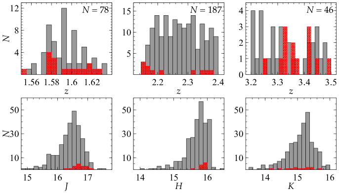
Figure 1: Distributions of the redshift estimate from SDSS (Lyke et al., 2020, Table D1, column 27 “Z”) in each redshift interval (top), and corresponding magnitude distributions (bottom). The initial GNIRS-DQS sample is marked in grey, and sources from the augmented sample are shown in red. The three redshift bins correspond to the H$\beta$ and [O iii] lines appearing at the center of the $J$, $H$, or $K$ photometric bands. The number of sources observed in each redshift bin is marked in each of the top panels. Of a total of 311 sources observed, 272 of which were reported in M21, usable NIR spectra were obtained for 260 sources ($\sim 84\%$ completion rate); the NIR spectra of 226 of these were presented in M21 and the remaining 34 are presented in this work.

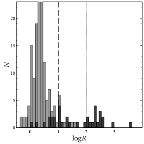
Figure 2: Radio-loudness distribution of the GNIRS-DQS sources. Darker shaded regions indicate new sources not in M21. The dashed line at log R = 1 indicates the threshold for radio-quiet quasars, and the dotted line at log R = 2 indicates the threshold for radio-loud quasars (see also M21).

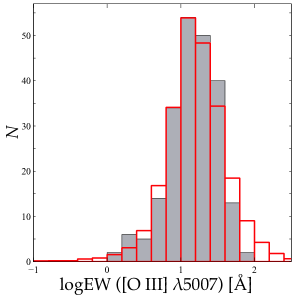
Figure 3: [O iii] $\lambda 5007$ rest-frame EW distribution of 220 GNIRS-DQS sources (solid gray histogram) and a similar distribution from Shen et al. (2011) (red outline; scaled down by a factor of 500). See M21 for additional discussion. Forty sources did not meet our threshold of reliability for an [O iii] EW measurement that we require to be greater than $1$ Å.

2.1 The Augmented GNIRS-DQS Catalog

We present spectroscopic observations for 34 sources that were observed in semester 2020B as part of our GNIRS-DQS campaign (see M21 for a detailed description of the observational strategy and the instrument configuration). We also include spectroscopic observations for 11 sources that were observed in a similar fashion, albeit with a narrower slit, 0.30^′′, in semester 2015A (program GN-2015A-Q-68; PI: Brotherton). Three of the 2020B sources, and one of the 2015A sources, were observed twice in their respective semesters. The log of these additional observations is given in Table 1.

Three of the 2020B observations were repeat observations of SDSS J094427.27+614424.6, SDSS J113924.64+332436.9, and SDSS J223934.45-004707.2, that were previously described in M21; the repeat observations were intended to improve the quality of the spectroscopic data for these three sources (see Table 1). Four of the 2020B observations, and 4 of the 2015A observations did not yielded adequate spectroscopic data, and are marked appropriately in Table 1. Therefore, in total, we have 37 useful observations, three of which are of sources that were already presented in M21. The augmented GNIRS-DQS catalog comprises of a total of 260 sources, 34 of which have been added in this work.

The formatting for the basic spectral properties of all 260 GNIRS-DQS objects is presented in Tables 2 and 3 in a similar fashion to Tables 2 and 3 in M21. The GNIRS-DQS sample was originally selected from the SDSS quasar catalogs for Data Release (DR) 12 and DR14 (Pâris et al., 2017, 2018); the augmented GNIRS-DQS catalog presented here includes 27 sources that were selected from SDSS DR16 (Lyke et al., 2020), which are marked appropriately in Table 1, and 7 sources from GN-2015A-Q-68 that were selected from SDSS DR7 (Schneider et al., 2010). DR16 measurements have been adopted for the full sample (Lyke et al., 2020). Table 4 presents the parameters used to model all of the emission lines, using Gaussian profiles, in the GNIRS-DQS spectra. For each profile, these parameters include the observed-frame wavelength of the line peak, velocity width (FWHM), and flux-density normalization ($f_{\lambda}$). All of the GNIRS spectra and their best-fit models are available electronically athttps://datalab.noirlab.edu/gnirs_dqs.php (catalog NOIRlab).

Table 1: GNIRS-DQS Observation Log

Quasar	$z_{\rm SDSS}$	$J$	$H$	$K$	Obs. Date	Net Exp.	Comments	BAL	RL
		[mag]	[mag]	[mag]		[s]
(1)	(2)	(3)	(4)	(5)	(6)	(7)	(8)	(9)	(10)
SDSS J001018.88+280932.5*	1.612	16.56	15.80	15.76	2020 Dec 09	1800	$\cdots$	$\cdots$	$\cdots$
SDSS J003001.11$-$015743.5	1.582	17.08	15.96	15.76	2020 Sep 09	1800	$\cdots$	$\cdots$	$\cdots$
SDSS J003853.15+333044.3	2.357	16.81	15.98	15.29	2020 Dec 25	1800	$\cdots$	$\cdots$	$\cdots$
SDSS J004613.54+010425.7	2.150	16.44	15.85	15.02	2020 Dec 11	1800	$\cdots$	1	$\cdots$
SDSS J004710.48+163106.5	2.165	16.33	15.62	14.90	2020 Dec 11	1800	$\cdots$	$\cdots$	$\cdots$
SDSS J005307.71+191022.7*	1.583	16.72	15.79	15.43	2020 Sep 08	1800	$\cdots$	$\cdots$	$\cdots$
SDSS J020329.86-091020.3*	1.579	17.02	15.97	15.64	2020 Aug 23	900	$\cdots$	$\cdots$	$\cdots$
	$\cdots$	$\cdots$	$\cdots$	$\cdots$	2020 Sep 11	900	$\cdots$	$\cdots$	$\cdots$
SDSS J073132.18+461347.0*	1.578	16.71	15.83	15.31	2020 Sep 29	1350	$\cdots$	$\cdots$	$\cdots$
SDSS J080117.91+333411.9*	1.598	16.73	15.99	15.79	2020 Oct 05	1350	$\cdots$	$\cdots$	$\cdots$
SDSS J080429.61+113013.9*	2.165	16.64	15.99	15.13	2020 Nov 27	1800	2	$\cdots$	$\cdots$
SDSS J080636.81+345048.5*	1.553	16.45	15.88	16.58	2020 Sep 30	1800	$\cdots$	1	$\cdots$
SDSS J080707.37+260729.1*	2.312	16.84	15.99	15.53	2020 Sep 30	1800	2	$\cdots$	$\cdots$
SDSS J081520.94+323512.9*	1.584	16.90	15.85	15.55	2020 Nov 28	1800	2	$\cdots$	$\cdots$
SDSS J084017.87+103428.8	3.330	16.69	16.47	15.27	2015 Apr 23	1720	$\cdots$	$\cdots$	$\cdots$
SDSS J084401.95+050357.9	3.350	15.39	14.93	14.19	2015 Apr 06	800	$\cdots$	$\cdots$	$\cdots$
SDSS J084526.75+550546.8*	1.620	16.33	15.65	15.18	2020 Nov 27	1800	$\cdots$	$\cdots$	$\cdots$
SDSS J091425.72+504854.9*	2.341	17.18	15.98	15.17	2020 Nov 29	1800	$\cdots$	$\cdots$	$\cdots$
SDSS J092942.97+064604.1*	1.608	16.65	15.53	15.28	2020 Nov 30	1800	$\cdots$	$\cdots$	$\cdots$
SDSS J094140.16+325703.2*	3.452	16.55	15.81	15.24	2020 Nov 29	1800	$\cdots$	$\cdots$	$\cdots$
SDSS J094427.27+614424.6*	2.340	16.41	15.61	14.72	2020 Dec 09	1800	3	$\cdots$	$\cdots$
SDSS J095047.45+194446.1*	1.575	16.80	15.98	15.62	2020 Dec 12	900	$\cdots$	$\cdots$	$\cdots$
	$\cdots$	$\cdots$	$\cdots$	$\cdots$	2020 Dec 21	900	$\cdots$	$\cdots$	$\cdots$
SDSS J095555.68+351652.6*	1.616	16.99	15.97	15.85	2020 Dec 09	1800	$\cdots$	$\cdots$	$\cdots$
SDSS J101724.26+333403.3*	1.579	16.49	15.84	15.40	2020 Nov 30	1800	$\cdots$	$\cdots$	$\cdots$
SDSS J111127.43+293319.3*	2.178	16.42	15.88	15.10	2020 Dec 31	1800	2	$\cdots$	$\cdots$
SDSS J112726.81+601020.2*	2.159	16.60	15.79	15.40	2020 Dec 31	2250	$\cdots$	$\cdots$	$\cdots$
SDSS J112938.46+440325.0*	2.213	16.99	15.88	15.11	2021 Jan 02	1800	$\cdots$	1	$\cdots$
SDSS J113330.17+144758.8*	3.248	16.90	15.88	15.64	2021 Jan 02	1800	$\cdots$	1	$\cdots$
SDSS J113924.64+332436.9*	2.314	16.38	15.95	14.85	2020 Dec 09	1800	3	$\cdots$	$\cdots$
SDSS J122343.15+503753.4	3.491	15.90	15.57	14.69	2015 Mar 30	1160	$\cdots$	$\cdots$	$\cdots$
SDSS J122938.61+462430.5*	2.152	16.30	15.77	15.19	2020 Nov 30	1800	$\cdots$	$\cdots$	$\cdots$
SDSS J130213.54+084208.6	3.305	16.12	15.64	15.02	2015 Apr 01	1720	2	$\cdots$	$\cdots$
SDSS J131048.17+361557.7	3.420	15.79	15.11	14.38	2015 Apr 05	800	2	$\cdots$	$\cdots$
SDSS J132845.00+510225.8	3.411	16.10	15.53	14.77	2015 Apr 05	1160	$\cdots$	$\cdots$	$\cdots$
SDSS J141321.05+092204.8	3.327	16.16	15.63	15.05	2015 Apr 05	1160	$\cdots$	$\cdots$	$\cdots$
SDSS J142123.97+463318.0	3.378	16.28	15.49	14.89	2015 Apr 07	1700	2	$\cdots$	$\cdots$
SDSS J142755.85$-$002951.1	3.362	16.60	15.91	15.27	2015 Apr 01	1720	$\cdots$	$\cdots$	$\cdots$
SDSS J165523.09+184708.4	3.327	16.28	15.88	15.19	2015 Apr 08	1720	2	$\cdots$	$\cdots$
SDSS J173352.23+540030.4	3.424	15.87	15.72	14.95	2015 Mar 23	1190	$\cdots$	$\cdots$	$\cdots$
	$\cdots$	$\cdots$	$\cdots$	$\cdots$	2015 Apr 01	680	$\cdots$	$\cdots$	$\cdots$
SDSS J210558.29$-$011127.5	1.625	16.61	15.49	15.54	2020 Aug 21	2250	1	$\cdots$	$\cdots$
SDSS J211251.06+000808.3*	1.618	16.85	15.89	15.89	2020 Aug 19	1800	1	$\cdots$	$\cdots$
SDSS J213655.35$-$080910.1	1.591	16.96	15.56	15.74	2020 Aug 23	1800	$\cdots$	$\cdots$	$\cdots$
SDSS J220139.99+114140.8*	2.382	16.87	15.76	15.84	2020 Aug 30	1800	1	$\cdots$	$\cdots$
SDSS J222310.76+180308.1*	1.602	16.70	15.99	15.60	2020 Sep 01	1800	1	$\cdots$	$\cdots$
SDSS J223934.45$-$004707.2	2.121	16.91	15.97	15.70	2020 Oct 03	1800	1, 3	$\cdots$	$\cdots$
SDSS J233304.61$-$092710.9	2.121	16.17	15.41	14.83	2021 Jan 01	1800	1	$\cdots$	$\cdots$
	$\cdots$	$\cdots$	$\cdots$	$\cdots$	2021 Jan 02	900	$\cdots$	$\cdots$	$\cdots$

Note. — Several sources have more than one observation, indicated by an empty source name. Only the 2020B and 2015A observations are shown. All 333 observations of GNIRS-DQS are available in the electronic version. All SDSS data taken from DR16.

Comments in Column (8) represent:

$[1]$ At least one exposure did not meet our observation conditions requirements.

$[2]$ Observation failed to provide spectrum of the source due to bad weather, instrument artifacts, or other technical difficulties during the observation.

$[3]$ Re-observed and updated from M21.

2.2 Improved Spectroscopic Inventory

Tables 2 and 3 include improved measurements of all spectral features. In particular, they include measurements of the rest-frame optical Fe ii emission blend which was fitted for each source in the same manner as in M21; however, each such feature now has a measured EW value and errors, thus effectively removing all the upper limits on the EWs (cf. Table 2 of M21). We fit two Gaussians to each broad emission-line profile to accommodate a possible asymmetry arising from, e.g., absorption, or outflows. We note that the two Gaussian fit per broad emission line is adopted only to characterize the line shape; the two Gaussians do not imply two physically distinct regions. The errors on the spectral measurements were calculated in the same manner as the other uncertainties described in M21, with upper and lower values being derived from a distribution of values recorded during the iterative process of broadening the Fe ii template (see M21 for a detailed description of the Fe ii blend fitting process).

In addition to the inclusion of 34 new sources, Tables 2 and 3 contain the most reliable data for the entire GNIRS-DQS sample following re-measurement of each spectrum with additional vetting and visual inspection, particularly with respect to the [O iii] and Fe ii fitting. These data therefore supersede the corresponding data presented in M21.

Table 2: Column Headings for Spectral Measurements

Column	Name	Bytes	Format	Units	Description
(1)	(2)	(3)	(4)	(5)	(6)
1	OBJ	(1-24)	A24	$\cdots$	SDSS object designation
2	ZSYS	(26-30)	F5.3	$\cdots$	Systemic redshifts
3	ZSRC	(32-34)	A3	$\cdots$	Emission line source for systemic redshift as described in M21
3	LC_MG II	(36-38)	I5	Å	Mg ii observed-frame wavelength
4	LC_MG II_UPP	(40-41)	I2	Å	Upper uncertainty for the line peak of Mg ii
5	LC_MG II_LOW	(43-44)	I2	Å	Lower uncertainty for the line peak of Mg ii
6	FWHM_MG II	(46-49)	I4	$\rm{km}$ $\rm{s^{-1}}$	FWHM of Mg ii
7	FWHM_MG II_UPP	(51-54)	I4	$\rm{km}$ $\rm{s^{-1}}$	Upper uncertainty of FWHM of Mg ii
8	FWHM_MG II_LOW	(56-59)	I4	$\rm{km}$ $\rm{s^{-1}}$	Lower uncertainty of FWHM of Mg ii
9	EW_MG II	(61-62)	I2	Å	Rest-frame EW of Mg ii
10	EW_MG II_UPP	(64-65)	I2	Å	Upper uncertainty of EW of Mg ii
11	EW_MG II_LOW	(67-68)	I2	Å	Lower uncertainty of EW of Mg ii
12	AS_MG II	(70-78)	E9.2	$\cdots$	Asymmetry of the double Gaussian fit profile of Mg ii
13	KURT_MG II	(80-83)	F4.2	$\cdots$	Kurtosis of the double Gaussian fit profile of Mg ii
14	LC_HB	(85-89)	I5	Å	H$\beta$ observed-frame wavelength
15	LC_HB_UPP	(91-92)	I2	Å	Upper uncertainty for the line peak of H$\beta$
16	LC_HB_LOW	(94-95)	I2	Å	Lower uncertainty for the line peak of H$\beta$
17	FWHM_HB	(97-101)	I5	$\rm{km}$ $\rm{s^{-1}}$	FWHM of H$\beta$
18	FWHM_HB_UPP	(103-107)	I5	$\rm{km}$ $\rm{s^{-1}}$	Upper uncertainty of FWHM of H$\beta$
19	FWHM_HB_LOW	(109-112)	I5	$\rm{km}$ $\rm{s^{-1}}$	Lower uncertainty of FWHM of H$\beta$
20	EW_HB	(114-116)	I3	Å	Rest-frame EW of H$\beta$
21	EW_HB_UPP	(118-119)	I2	Å	Upper uncertainty of EW of H$\beta$
22	EW_HB_LOW	(121-122)	I2	Å	Lower uncertainty of EW of H$\beta$
23	AS_HB	(124-132)	E9.2	$\cdots$	Asymmetry of the double Gaussian fit profile of H$\beta$
24	KURT_HB	(134-137)	F4.2	$\cdots$	Kurtosis of the double Gaussian fit profile of H$\beta$
25	LC_O III	(139-143)	I5	Å	[O iii] $\lambda$5007 observed-frame wavelength
26	LC_O III_UPP	(145-146)	I2	Å	Upper uncertainty for the line peak of [O iii] $\lambda$5007
27	LC_O III_LOW	(148-149)	I2	Å	Lower uncertainty for the line peak of [O iii] $\lambda$5007
28	FWHM_O III	(151-154)	I4	$\rm{km}$ $\rm{s^{-1}}$	FWHM of [O iii] $\lambda$5007
29	FWHM_O III_UPP	(156-159)	I4	$\rm{km}$ $\rm{s^{-1}}$	Upper uncertainty of FWHM of [O iii] $\lambda$5007
30	FWHM_O III_LOW	(161-164)	I4	$\rm{km}$ $\rm{s^{-1}}$	Lower uncertainty of FWHM of [O iii] $\lambda$5007
31	EW_O III	(166-173)	E8.2	Å	Rest-frame EW of [O iii] $\lambda$5007
32	EW_O III_UPP	(175-182)	E8.2	Å	Upper uncertainty of EW of [O iii] $\lambda$5007
33	EW_O III_LOW	(184-191)	E8.2	Å	Lower uncertainty of EW of [O iii] $\lambda$5007
34	AS_O III	(193-201)	E9.2	$\cdots$	Asymmetry of the double Gaussian fit profile of [O iii] $\lambda$5007
35	KURT_O III	(203-206)	F4.2	$\cdots$	Kurtosis of the double Gaussian fit profile of [O iii] $\lambda$5007
36	LC_HA	(208-212)	I5	Å	H$\alpha$ observed-frame wavelength
37	LC_HA_UPP	(214-215)	I2	Å	Upper uncertainty for the line peak of H$\alpha$
38	LC_HA_LOW	(217-218)	I2	Å	Lower uncertainty for the line peak of H$\alpha$
39	FWHM_HA	(220-223)	I4	$\rm{km}$ $\rm{s^{-1}}$	FWHM of H$\alpha$
40	FWHM_HA_UPP	(225-228)	I4	$\rm{km}$ $\rm{s^{-1}}$	Upper uncertainty of FWHM of H$\alpha$
41	FWHM_HA_LOW	(230-233)	I4	$\rm{km}$ $\rm{s^{-1}}$	Lower uncertainty of FWHM of H$\alpha$
42	EW_HA	(235-237)	I3	Å	Rest-frame EW of H$\alpha$
43	EW_HA_UPP	(239-240)	I2	Å	Upper uncertainty of EW of H$\alpha$
44	EW_HA_LOW	(242-243)	I2	Å	Lower uncertainty of EW of H$\alpha$
45	AS_HA	(245-253)	E9.2	$\cdots$	Asymmetry of the double Gaussian fit profile of H$\alpha$
46	KURT_HA	(255-258)	F4.2	$\cdots$	Kurtosis of the double Gaussian fit profile of H$\alpha$
47	FWHM_FE II	(260-264)	F5.0	$\rm{km}$ $\rm{s^{-1}}$	FWHM of the kernel Gaussian used to broaden the Fe ii template
48	EW_FE II	(266-273)	E8.2	Å	Rest-frame EW of optical band Fe ii as defined by Boroson & Green (1992)
49	EW_FE II_UPP	(275-282)	E8.2	Å	Upper uncertainty of EW of Fe ii
50	EW_FE II_LOW	(284-291)	E8.2	Å	Lower uncertainty of EW of Fe ii
51	LOGF$\lambda$5100	(293-298)	F6.2	$\rm{erg}\ \rm{s^{-1}}\rm{cm^{-2}}\rm{\AA^{-1}}$	Flux density at rest-frame 5100 Å
52	LOGL5100	(300-304)	F5.2	$\rm{erg}$ $\rm{s^{-1}}$ $\rm\AA^{-1}$	Monochromatic luminosity at rest-frame 5100 Å based on $z_{\rm sys}$

Note. — Data formatting used for the catalog. Asymmetry is defined here as the skewness of the Gaussian fits, i.e., a measure of the asymmetry of the distribution about its mean, $s=E(x-\mu)^{3}/\sigma^{3}$, where $\mu$  is the mean of $x$, $\sigma$  is the standard deviation of $x$, and $E(t)$ is the expectation value. Kurtosis is the quantification of the ”tails” of the Gaussian fits defined as $k=E(x-\mu)^{4}/\sigma^{4}$. All of the GNIRS spectra and their best-fit models are available electronically athttps://datalab.noirlab.edu/gnirs_dqs.php (catalog https://datalab.noirlab.edu/gnirs_dqs.php).

Table 3: Column Headings for Supplemental Emission-Line Measurements

Column	Name	Bytes	Format	Units	Description
(1)	(2)	(3)	(4)	(5)	(6)
1	OBJ	(1-24)	A24	$\cdots$	SDSS object designation
2	LC_HD	(26-30)	I5	Å	H$\delta$ observed-frame wavelength
3	LC_HD_UPP	(32-33)	I2	Å	Upper uncertainty for the line peak of H$\delta$
4	LC_HD_LOW	(35-36)	I2	Å	Lower uncertainty for the line peak of H$\delta$
5	FWHM_HD	(38-41)	I4	$\rm{km}$ $\rm{s^{-1}}$	FWHM of H$\delta$
6	FWHM_HD_UPP	(43-45)	I3	$\rm{km}$ $\rm{s^{-1}}$	Upper uncertainty of FWHM of H$\delta$
7	FWHM_HD_LOW	(47-49)	I3	$\rm{km}$ $\rm{s^{-1}}$	Lower uncertainty of FWHM of H$\delta$
8	EW_HD	(51-52)	I2	Å	Rest-frame EW of H$\delta$
9	EW_HD_UPP	(54-55)	I2	Å	Upper uncertainty of EW of H$\delta$
10	EW_HD_LOW	(57-58)	I2	Å	Lower uncertainty of EW of H$\delta$
11	AS_HD	(60-68)	E9.2	$\cdots$	Asymmetry of the double Gaussian fit profile of H$\delta$
12	KURT_HD	(70-73)	F4.2	$\cdots$	Kurtosis of the double Gaussian fit profile of H$\delta$
13	LC_HG	(75-79)	I5	Å	H$\gamma$ observed-frame wavelength
14	LC_HG_UPP	(81-82)	I2	Å	Upper uncertainty for the line peak of H$\gamma$
15	LC_HG_LOW	(84-85)	I2	Å	Lower uncertainty for the line peak of H$\gamma$
16	FWHM_HG	(87-90)	I4	$\rm{km}$ $\rm{s^{-1}}$	FWHM of H$\gamma$
17	FWHM_HG_UPP	(92-95)	I4	$\rm{km}$ $\rm{s^{-1}}$	Upper uncertainty of FWHM of H$\gamma$
18	FWHM_HG_LOW	(97-100)	I4	$\rm{km}$ $\rm{s^{-1}}$	Lower uncertainty of FWHM of H$\gamma$
19	EW_HG	(102-103)	I2	Å	Rest-frame EW of H$\gamma$
20	EW_HG_UPP	(105-106)	I2	Å	Upper uncertainty of EW of H$\gamma$
21	EW_HG_LOW	(108-109)	I2	Å	Lower uncertainty of EW of H$\gamma$
22	AS_HG	(111-119)	E9.2	$\cdots$	Asymmetry of the double Gaussian fit profile of H$\gamma$
23	KURT_HG	(121-124)	F4.2	$\cdots$	Kurtosis of the double Gaussian fit profile of H$\gamma$
24	LC_O II	(126-130)	I5	Å	[O ii] observed-frame wavelength
25	LC_O II_UPP	(132-133)	I2	Å	Upper uncertainty for the line peak of [O ii]
26	LC_O II_LOW	(135-136)	I2	Å	Lower uncertainty for the line peak of [O ii]
27	FWHM_O II	(138-141)	I4	$\rm{km}$ $\rm{s^{-1}}$	FWHM of [O ii]
28	FWHM_O II_UPP	(143-147)	I5	$\rm{km}$ $\rm{s^{-1}}$	Upper uncertainty of FWHM of [O ii]
29	FWHM_O II_LOW	(149-152)	I4	$\rm{km}$ $\rm{s^{-1}}$	Lower uncertainty of FWHM of [O ii]
30	EW_O II	(154-155)	I2	Å	Rest-frame EW of [O ii]
31	EW_O II_UPP	(157-158)	I2	Å	Upper uncertainty of EW of [O ii]
32	EW_O II_LOW	(160-161)	I2	Å	Lower uncertainty of EW of [O ii]
33	AS_O II	(163-171)	E9.2	$\cdots$	Asymmetry of the double Gaussian fit profile of [O ii]
34	KURT_O II	(173-176)	F4.2	$\cdots$	Kurtosis of the double Gaussian fit profile of [O ii]
35	LC_NE III	(178-182)	I5	Å	[Ne iii] observed-frame wavelength
36	LC_NE III_UPP	(184-185)	I2	Å	Upper uncertainty for the line peak of [Ne iii]
37	LC_NE III_LOW	(187-188)	I2	Å	Lower uncertainty for the line peak of [Ne iii]
38	FWHM_NE III	(190-193)	I4	$\rm{km}$ $\rm{s^{-1}}$	FWHM of [Ne iii]
39	FWHM_NE III_UPP	(195-198)	I4	$\rm{km}$ $\rm{s^{-1}}$	Upper uncertainty of FWHM of [Ne iii]
40	FWHM_NE III_LOW	(200-203)	I4	$\rm{km}$ $\rm{s^{-1}}$	Lower uncertainty of FWHM of [Ne iii]
41	EW_NE III	(205-206)	I2	Å	Rest-frame EW of [Ne iii]
42	EW_NE III_UPP	(208-209)	I2	Å	Upper uncertainty of EW of [Ne iii]
43	EW_NE III_LOW	(211-212)	I2	Å	Lower uncertainty of EW of [Ne iii]
44	AS_NE III	(214-222)	E9.2	$\cdots$	Asymmetry of the double Gaussian fit profile of [Ne iii]
45	KURT_NE III	(224-227)	F4.2	$\cdots$	Kurtosis of the double Gaussian fit profile of [Ne iii]

Note. — Data formatting used for the supplemental measurements in the supplemental features catalog.

Table 4: Column Headings for Gaussian Parameters of Emission-Line Profiles

Column	Name	Bytes	Format	Units	Description
(1)	(2)	(3)	(4)	(5)	(6)
1	OBJ	(1-24)	A24	$\cdots$	SDSS object designation
2	MG II_LAM_PEAK_NARROW	(26-29)	I4	Å	Narrow Mg ii  peak
3	MG II_STD_NARROW	(31-32)	I2	Å	Narrow Mg ii  width
4	MG II_F_LAM_NARROW	(34-37)	I4	$\rm{erg}\ \rm{s^{-1}}\rm{cm^{-2}}\rm{\AA^{-1}}$	Narrow Mg ii  normalization
5	MG II_LAM_PEAK_BROAD	(39-42)	I4	Å	Broad Mg ii  peak
6	MG II_STD_BROAD	(44-47)	I4	Å	Broad Mg ii  width
7	MG II_F_LAM_BROAD	(49-52)	I4	$\rm{erg}\ \rm{s^{-1}}\rm{cm^{-2}}\rm{\AA^{-1}}$	Broad Mg ii  normalization
8	O II_LAM_PEAK_NARROW	(54-57)	I4	Å	Narrow [O ii]  peak
9	O II_STD_NARROW	(59-60)	I2	Å	Narrow [O ii]  width
10	O II_F_LAM_NARROW	(62-65)	I4	$\rm{erg}\ \rm{s^{-1}}\rm{cm^{-2}}\rm{\AA^{-1}}$	Narrow [O ii]  normalization
11	O II_LAM_PEAK_BROAD	(67-70)	I4	Å	Broad [O ii]  peak
12	O II_STD_BROAD	(72-75)	I4	Å	Broad [O ii]  width
13	O II_F_LAM_BROAD	(77-78)	I2	$\rm{erg}\ \rm{s^{-1}}\rm{cm^{-2}}\rm{\AA^{-1}}$	Broad [O ii]  normalization
14	NE III_LAM_PEAK_NARROW	(80-83)	I4	Å	Narrow [Ne iii]  peak
15	NE III_STD_NARROW	(85-86)	I2	Å	Narrow [Ne iii]  width
16	NE III_F_LAM_NARROW	(88-89)	I2	$\rm{erg}\ \rm{s^{-1}}\rm{cm^{-2}}\rm{\AA^{-1}}$	Narrow [Ne iii]  normalization
17	NE III_LAM_PEAK_BROAD	(91-94)	I4	Å	Broad [Ne iii]  peak
18	NE III_STD_BROAD	(96-99)	I4	Å	Broad [Ne iii]  width
19	NE III_F_LAM_BROAD	(101-102)	I2	$\rm{erg}\ \rm{s^{-1}}\rm{cm^{-2}}\rm{\AA^{-1}}$	Broad [Ne iii]  normalization
20	HD_LAM_PEAK_NARROW	(104-107)	I4	Å	Narrow H$\delta$  peak
21	HD_STD_NARROW	(109-110)	I2	Å	Narrow H$\delta$  width
22	HD_F_LAM_NARROW	(112-113)	I2	$\rm{erg}\ \rm{s^{-1}}\rm{cm^{-2}}\rm{\AA^{-1}}$	Narrow H$\delta$  normalization
23	HD_LAM_PEAK_BROAD	(115-118)	I4	Å	Broad H$\delta$  peak
24	HD_STD_BROAD	(120-123)	I4	Å	Broad H$\delta$  width
25	HD_F_LAM_BROAD	(125-127)	I3	$\rm{erg}\ \rm{s^{-1}}\rm{cm^{-2}}\rm{\AA^{-1}}$	Broad H$\delta$  normalization
26	HG_LAM_PEAK_NARROW	(129-132)	I4	Å	Narrow H$\gamma$  peak
27	HG_STD_NARROW	(134-135)	I2	Å	Narrow H$\gamma$  width
28	HG_F_LAM_NARROW	(137-139)	I3	$\rm{erg}\ \rm{s^{-1}}\rm{cm^{-2}}\rm{\AA^{-1}}$	Narrow H$\gamma$  normalization
29	HG_LAM_PEAK_BROAD	(141-144)	I4	Å	Broad H$\gamma$  peak
30	HG_STD_BROAD	(146-149)	I4	Å	Broad H$\gamma$  width
31	HG_F_LAM_BROAD	(151-153)	I3	$\rm{erg}\ \rm{s^{-1}}\rm{cm^{-2}}\rm{\AA^{-1}}$	Broad H$\gamma$  normalization
32	HB_LAM_PEAK_NARROW	(155-158)	I4	Å	Narrow H$\beta$  peak
33	HB_STD_NARROW	(160-162)	I3	Å	Narrow H$\beta$  width
34	HB_F_LAM_NARROW	(164-166)	I3	$\rm{erg}\ \rm{s^{-1}}\rm{cm^{-2}}\rm{\AA^{-1}}$	Narrow H$\beta$  normalization
35	HB_LAM_PEAK_BROAD	(168-171)	I4	Å	Narrow H$\beta$  peak
36	HB_STD_BROAD	(173-175)	I3	Å	Broad H$\beta$  width
37	HB_F_LAM_BROAD	(177-179)	I3	$\rm{erg}\ \rm{s^{-1}}\rm{cm^{-2}}\rm{\AA^{-1}}$	Broad H$\beta$  normalization
38	O III_1_LAM_PEAK_NARROW	(181-184)	I4	Å	Narrow [O iii] 4959Å  peak
39	O III_1_STD_NARROW	(186-187)	I2	Å	Narrow [O iii] 4959Å  width
40	O III_1_F_LAM_NARROW	(189-191)	I3	$\rm{erg}\ \rm{s^{-1}}\rm{cm^{-2}}\rm{\AA^{-1}}$	Narrow [O iii] 4959Å  normalization
41	O III_1_LAM_PEAK_BROAD	(193-196)	I4	Å	Broad [O iii] 4959Å  peak
42	O III_1_STD_BROAD	(198-200)	I3	Å	Broad [O iii] 4959Å  width
43	O III_1_F_LAM_BROAD	(202-204)	I3	$\rm{erg}\ \rm{s^{-1}}\rm{cm^{-2}}\rm{\AA^{-1}}$	Broad [O iii] 4959Å  normalization
44	O III_2_LAM_PEAK_NARROW	(206-209)	I4	Å	Narrow [O iii] 5007Å  peak
45	O III_2_STD_NARROW	(211-212)	I2	Å	Narrow [O iii] 5007Å  width
46	O III_2_F_LAM_NARROW	(214-216)	I3	$\rm{erg}\ \rm{s^{-1}}\rm{cm^{-2}}\rm{\AA^{-1}}$	Narrow [O iii] 5007Å  normalization
47	O III_2_LAM_PEAK_BROAD	(218-221)	I4	Å	Broad [O iii] 5007Å  peak
48	O III_2_STD_BROAD	(223-225)	I3	Å	Broad [O iii] 5007Å  width
49	O III_2_F_LAM_BROAD	(227-229)	I3	$\rm{erg}\ \rm{s^{-1}}\rm{cm^{-2}}\rm{\AA^{-1}}$	Broad [O iii] 5007Å  normalization
50	HA_LAM_PEAK_NARROW	(231-234)	I4	Å	Narrow H$\alpha$  peak
51	HA_STD_NARROW	(236-238)	I3	Å	Narrow H$\alpha$  width
52	HA_F_LAM_NARROW	(240-243)	I4	$\rm{erg}\ \rm{s^{-1}}\rm{cm^{-2}}\rm{\AA^{-1}}$	Narrow H$\alpha$  normalization
53	HA_LAM_PEAK_BROAD	(245-248)	I4	Å	Broad H$\alpha$  peak
54	HA_STD_BROAD	(250-252)	I3	Å	Broad H$\alpha$  width
55	HA_F_LAM_BROAD	(254-256)	I3	$\rm{erg}\ \rm{s^{-1}}\rm{cm^{-2}}\rm{\AA^{-1}}$	Broad H$\alpha$  normalization

Note. — Independent Gaussian feature fit parameters for each emission line that was fit with both a narrow and broad Gaussian profile.

2.3 C iv Emission-Line Measurements

M17 and D20 found that the accuracy and precision of a source’s UV-based redshift can be significantly improved when regressed against the FWHM and EW of its C iv line as well as the UV continuum luminosity at a rest-frame wavelength of 1350Å ($L_{\rm 1350}$). The C iv emission line has been measured in the SDSS spectrum of each GNIRS-DQS source using the same fitting approach outlined in D20, which closely follows the methods utilized in both M21 and this work; the C iv emission-line properties of all the GNIRS-DQS sources appear in Paper II.

3 Correcting UV-Based Redshifts

Our aim is to derive corrections that, on average, shift the velocity offsets of the UV-based redshifts as close as possible to a velocity offset of zero $\rm{km~{}s^{-1}}$ from $z_{\rm sys}$ based on the [O iii] $\lambda 5007$ line. We derive this correction by applying a regression analysis to a calibration sample of 121 sources from GNIRS-DQS as described below.

The sample used for this analysis is a subset of the augmented GNIRS-DQS sample described in Section 2. Starting with the 260 GNIRS-DQS sources with useful NIR spectra, we include only the 220 objects with [O iii] rest-frame EW measurements greater than 1 Å that can provide the most accurate values of $z_{\rm sys}$ (see Figure 3); i.e., 40 sources whose $z_{\rm sys}$ values were based on either Mg ii or H$\beta$ were removed. We then remove 52 broad absorption line (BAL) quasars, identified as such based on criteria outlined in their respective source catalogs using “balnicity” index and visual inspection (see, Gibson et al., 2009; Shen et al., 2011; Pâris et al., 2017, 2018; Lyke et al., 2020), as the BAL troughs often degrade measurements of the EW and FWHM for C iv, which are of primary importance for our regression analysis (e.g., Begelman et al., 1991; Gibson et al., 2009). We also remove 17 radio-loud (RL) quasars (having $R>100$; see Figure 2), one of which, SDSS J114705.24+083900.6, is also classified as a BAL quasar, due to potential continuum boosting, which may affect both EW (C iv) and $L_{1350}$ measurements (e.g., Miller et al., 2011).

Two additional sources, SDSS J073132.18+461347.0, and SDSS J141617.38+264906.1, were excluded due to the inability to measure the C iv line reliably (see Paper II). Finally, 29 objects were removed from the sample due to additional visual inspection and a lack of a prominent [O iii] $\lambda$5007 emission line. The result of this selection process is a calibration sample of 121 sources, presented in Table 5, which is a representative sample of optically selected quasars (see Section 2) used to derive prescriptions for correcting UV-based redshifts through linear regression analysis.

Table 5: Redshifts and Velocity Offsets

			$\Delta v_{i}$		$\Delta v_{i}$		$\Delta v_{i}$
Quasar	$z_{\rm sys}$	$z_{\rm C\,IV}$	($\rm{km~{}s^{-1}}$)	$z_{\rm HW10}$	($\rm{km~{}s^{-1}}$)	$z_{\rm Pipe}$	($\rm{km~{}s^{-1}}$)
SDSS J001018.88+280932.5	1.613	1.611	-230	$\cdots$	$\cdots$	1.612	-110
SDSS J001453.20+091217.6	2.340	2.326	-1250	2.344	340	2.308	-2840
SDSS J001914.46+155555.9	2.267	2.263	-370	2.276	830	2.271	350
SDSS J002634.46+274015.5	2.247	2.243	-340	2.247	50	2.267	1850
SDSS J003001.11$-$015743.5	1.588	1.579	-1030	1.590	200	1.582	-710
SDSS J003416.61+002241.1	1.631	1.626	-560	1.630	-50	1.627	-410
SDSS J004710.48+163106.5	2.192	2.162	-2770	$\cdots$	$\cdots$	2.165	-2490
SDSS J004719.71+014813.9	1.591	1.588	-340	1.590	-130	1.590	-130
SDSS J005233.67+014040.8	2.309	2.295	-1250	2.305	-370	2.291	-1620
SDSS J005307.71+191022.7	1.598	1.581	-1940	1.585	-1460	1.583	-1680

Note. — Complete table of 121 sources appears in the electronic version.

The redshift corrections are performed on redshifts obtained using three separate techniques: 1) measurements of the observed-frame wavelength of the peak of the C iv emission line, 2) HW10 redshifts (P. Hewett, priv. comm.), and 3) SDSS Pipeline redshifts (Bolton et al., 2012, Table D1, column 29 “Z_PIPE”). The HW10 redshifts are notable as they already have a primary redshift correction applied.

The principal metric under investigation in this work is the initial velocity offset ($\Delta v_{i}$) between each of the aforementioned three UV-based redshifts ($z_{\rm meas}$) and the $z_{\rm sys}$ value of a source determined from its [O iii] $\lambda 5007$ emission line by measuring the line peak in each spectrum, which is presented in Table 2. This offset is computed using the following equation (see D20):

$$\Delta v_{i}=c\left(\frac{z_{\rm meas}-z_{\rm sys}}{1+z_{\rm sys}}\right).$$ (1)

These initial velocity offset values are presented in Table 5 and are shown in the top panels of Figure 4.

As shown in Table 5, there is one source, SDSS J090247.57+304120.7, where the SDSS Pipeline produces an erroneous redshift, resulting in an unrealistically high velocity offset of $|\Delta\it{v_{i}}|>\rm{16000}~{}\rm{km~{}s^{-1}}$, while the velocity offsets for this source from the C iv and HW10 methods yield values that are only $-170$ and $+70~{}\rm{km~{}s^{-1}}$, respectively. As a result, this source is excluded from the SDSS Pipeline analysis, but is retained in the C iv and HW10 analyses.

It is known that the C iv velocity offsets are correlated with the C iv FWHM (e.g., Coatman et al., 2017). However, as was discovered by M17 and D20, additional corrections to the velocity offsets can be obtained by including two additional parameters: EW(C iv) and $L_{1350}$. In this work, we confirm that all three parameters, FWHM(C iv), EW(C iv), and $L_{1350}$, are required for obtaining the best corrections for the velocity offsets in the following manner:

$$\Delta v_{\rm corr}~{}(\rm{km~{}s^{-1}})=\alpha\rm{logFWHM_{CIV}}~{}(\rm{km~{}s^{-1}})\\ +\ \beta\rm{logEW_{CIV}}~{}(\AA)\\ +\ \gamma\rm{log\it{L}_{\rm 1350}}\ (10^{-17}\ erg\ s^{-1}\AA^{-1})$$ (2)

where $\Delta v_{\rm corr}$ is the velocity offset we subtract from the initial velocity offset calculated using Equation 1.

The final, post-correction velocity offset, $\Delta v_{f}=\Delta v_{i}-\Delta v_{\rm corr}$, is displayed in the bottom panels of Figure 4. Since the goal of Equation 2 is to eliminate the velocity offsets, then, by definition, the mean ($\mu$) of $\Delta v_{i}-\Delta v_{corr}$ is zero. This $\Delta v_{\rm corr}$ value is used to obtain a revised $z_{\rm{sys}}$ prediction by adjusting the initially measured redshift of a quasar. From Equation 1, solving for $z_{\rm meas}$, and substituting $z_{\rm meas}$ = $z_{\rm sys}$ and $v_{\rm corr}$ = $v_{i}$, we get

$$z_{\rm rev}=z_{\rm meas}+\frac{\Delta v_{\rm corr}(1+z_{\rm meas})}{c}$$ (3)

where $z_{\rm rev}$ is the revised, more accurate, and more precise redshift.

Starting with our 121-source calibration sample, we run linear regressions using the three parameters defined in Equation 2. The results provide the $\Delta v_{\rm corr}$ values from Equation 2 that are subtracted from the initial velocity offsets of the sources (from Table 5).

Distributions of the $\Delta v_{i}$ and $\Delta v_{f}$ values are plotted in the top and bottom panels in Figure 4, respectively. We observe that the C iv-based $\Delta v_{i}$ values are skewed toward negative values (blueshifts) with a mean velocity offset of $\mu=-864~{}\rm{km~{}s^{-1}}$, and a standard deviation of $\sigma=804~{}\rm{km~{}s^{-1}}$. The SDSS Pipeline-based $\Delta v_{i}$ values have a considerably smaller negative initial velocity offset of $\mu=-443~{}\rm{km~{}s^{-1}}$, yet a larger standard deviation of $\sigma=883~{}\rm{km~{}s^{-1}}$. As expected, the HW10-based $\Delta v_{i}$ values show a mean initial velocity offset much closer to zero ($\mu=92~{}\rm{km~{}s^{-1}}$), with the standard deviation being notably smaller than that of the C iv-based $\Delta v_{i}$ values ($\sigma=679~{}\rm{km~{}s^{-1}}$). Despite the improvements demonstrated by the HW10-based values, we are able to use our regression analysis to improve on UV-based redshift determinations further, as shown below.

As explained above, our redshift corrections yield mean $\Delta v_{f}$ values of zero $\rm{km~{}s^{-1}}$ using all three UV-based methods (see the bottom panels of Figure 4). The standard deviations ($\sigma$) of the $\Delta v_{f}$ values, on the other hand, are reduced by $\sim 18\%$, $\sim 2\%$, and $\sim 7\%$ for the C iv, HW10, and SDSS Pipeline methods, respectively, with respect to the measured $\Delta v_{i}$ values. The median velocity offsets are also reduced significantly for all three methods. The linear regression coefficients (Equation 2) used to achieve these corrections are presented in Table 6. The uncertainties on the coefficients, shown in Table 6, from the regression defined in Equation 2 stem directly from the mean squared error from the linear fit. These uncertainties (translated to $\sim 700~{}\rm{km~{}s^{-1}}$ in velocity space; see Figure 4) are considerably larger than the intrinsic uncertainties associated with the [O iii] line wavelength calibration (on the order of $\sim 10~{}\rm{km~{}s^{-1}}$; see M21) or the deviation of the [O iii] line from the systemic redshift ($-48~{}\rm{km~{}s^{-1}}$ systematic offset, and $56~{}\rm{km~{}s^{-1}}$ uncertainty; Shen et al. 2016); therefore we adopt the regression uncertainties as the most conservative error estimates. Table 6 also gives the t-Value (e.g., Sheskin, 2007) for confidence statistics in determining the importance of each parameter (see also D20), where t-Values of $|t|\gtrsim 2$ denote a strong correlation, with decreasing confidence as $t\rightarrow 0$.

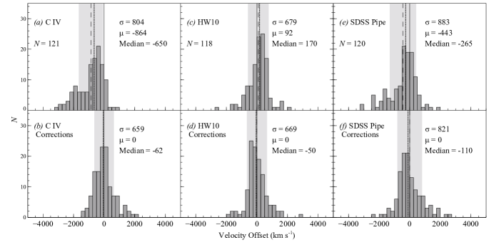
Figure 4: Velocity offsets relative to $z_{\rm{sys}}$ before (panels a, c, and e) and after (panels b, d, and f) the corrections using the linear regression coefficients given in Table 6. The standard deviation (shaded region), mean (dashed line), median (dotted line), and zero velocity offset (solid line) are marked in each panel. SDSS J090247.57+304120.7 does not appear on the SDSS Pipe panels due to its erroneous redshift. The mean ($\mu$), median, and standard deviation ($\sigma$) given in units of$~{}\rm{km~{}s^{-1}}$, are noted in each panel. The number of sources used in each regression analysis ($N$) is given in the upper panels.

Table 6: Linear Regression Coefficients

UV-Based	Sample	Regression	Value	Error	$t$-Value
Redshift Method	Size	Coefficients
		$\alpha$	-2589	428	-6.05
C iv	121	$\beta$	1156	292	3.95
		$\gamma$	148	36	4.15
		$\alpha$	-587	389	-1.51
HW10	118	$\beta$	283	261	1.09
		$\gamma$	39	32	1.21
		$\alpha$	9371	8557	1.10
SDSS Pipe	120	$\beta$	-3694	5851	-0.63
		$\gamma$	-655	715	-0.92

Residuals of the 121 source sample both before and after our corrections are applied are presented in Figure 5. The residual distributions show the substantial reduction in the velocity offsets before and after each correction. The corrected velocity offsets for both the C iv and HW10-based methods are closer to zero than the corrected velocity offsets for the SDSS Pipeline method.

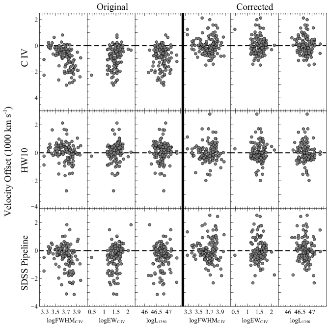
Figure 5: Residual velocity offsets with respect to $z_{\rm sys}$ before (three leftmost columns), and after (three rightmost columns), corrections are applied (see Equation 2) against our regression parameters. SDSS J090247.57+304120.7 does not appear in the SDSS Pipeline panels due to its erroneously reported redshift, as discussed in Section 3.

The relatively small improvement in the mean velocity offset ($\mu$), and the standard deviation ($\sigma$), achieved for the HW10 method is likely related to the fact that our analysis constitutes a second-order correction to the one already employed by HW10; this result reinforces the general reliability of that method. The C iv-based redshifts, while based solely on a single emission line, provide a slightly smaller standard deviation than the HW10-based method when corrected using our regression analysis (see Figure 4). Finally, the SDSS Pipeline-based redshifts provide the least reliable results; in particular, we find that the SDSS Pipeline fails to produce a meaningful redshift for one out of 121 sources in our calibration sample (SDSS J090247.57+304120.7). Furthermore, DR16 redshifts (Lyke et al., 2020, Table D1, column 10 “$\rm{Z}\_\rm{QN}$”) available for 101 sources from our sample provide significantly larger standard deviations than the SDSS Pipeline values both before and after the correction.

For our calibration sample, the largest $\Delta v_{i}$ value is on the order of $\sim-3000~{}\rm{km~{}s^{-1}}$, with a few sources having velocity offsets within the $-3000~{}\rm{km~{}s^{-1}}$ $\lesssim\Delta v_{i}\lesssim$ $-2000~{}\rm{km~{}s^{-1}}$ range. Values of this magnitude, while high, are not unexpected due to the kinematics associated with luminous, rapidly accreting quasars that can directly affect the C iv emission line and cause large blueshifts (e.g., Murray et al., 1995; Sulentic et al., 2007; Shen et al., 2008; Dix et al., 2020). Panel $(a)$ of Figure 4, and to a lesser extent panel $(e)$, demonstrate the impact of this effect via the asymmetric distribution caused by this large range of velocity offsets. Nevertheless, our method tends to correct even these large velocity offsets to more reasonable values as shown in Figures 4 and 6.

Our velocity offset distributions may appear more asymmetric with respect to previous studies of this kind. For example, Shen et al. (2011), who derived C iv velocity offsets based on Mg ii (from the same SDSS spectrum), provide more symmetric distributions than those presented in Figure 4. This may be a result of the much larger uncertainties in the determination of $z_{\rm sys}$ from Mg ii that was used in that study, compared with the uncertainties associated with the [O iii] lines, which are up to an order of magnitude smaller (e.g., M21).

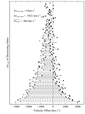
Figure 6: Initial velocity offsets ($\Delta v_{i}$; circles) compared to final velocity offsets ($\Delta v_{f}$; squares) for C iv-based redshifts of the calibration sample of 121 sources. The lines connecting the initial and final velocity offsets are sorted from top to bottom by the absolute value of the velocity offset correction ($|\Delta v_{\rm corr}|$). Solid lines, dashed lines, and dotted lines refer to the following luminosity ranges: $46.08<$ log($L_{5100}$) $<46.41$, $46.42<$ log($L_{5100}$) $<46.74$, and $46.75<~{}$log($L_{5100}$) $<47.09$, respectively. Fifteen sources have $|\Delta v_{\rm corr}|<100~{}\rm{km~{}s^{-1}}$, 11, three, and one of which belong to the lowest, medium, and highest luminosity ranges, respectively. While the majority of the $\Delta v_{i}$ values, which are blueshifts, produce $\Delta v_{f}$ values with the opposite sign, we also see $\Delta v_{i}$ values which are redshifts that end up as blueshifts; however the overall effect of our regression analysis brings $\Delta v_{f}$ values closer to zero. We find no trend between $|\Delta v_{\rm corr}|$ and the monochromatic luminosity at rest-frame 5100 Å.

The results of our regression analysis, presented in Table 6, provide considerably improved redshifts over the regression coefficients used by D20. When we employ the D20 regression coefficients on our calibration sample of 121 sources, we obtain standard deviations for the distributions of $\Delta v_{f}$ which are $\sim 18\%$ larger for the HW10 method, $\sim 32\%$ larger for the SDSS Pipeline method, and $\sim 4\%$ larger for the C iv-based redshifts compared to using the coefficients from Table 6. In summary, considering the four basic observables associated with the C iv emission line, one can derive the most accurate and precise prediction of the systemic redshift of a quasar using that sole emission line.

3.1 Redshift and Luminosity Dependence

Typically, redshifts are determined either spectroscopically or photometrically from multiple features (i.e., HW10 and the SDSS Pipeline). When some of these features are no longer available in a spectrum, our ability to determine the redshift is affected, and it is plausible that the initial velocity offsets depend also on source redshift. We search for such a dependence in our data by splitting our calibration sample into three redshift bins: $1.55\lesssim z\lesssim 1.65$ (Bin 1), $2.10\lesssim z\lesssim 2.40$ (Bin 2), and $3.20\lesssim z\lesssim 3.50$ (Bin 3), which contain 37, 71, and 13 sources, respectively. These intervals ensure coverage of the [O iii] $\lambda 5007$ emission line in the $J$, $H$, or $K$ bands, respectively (see Section 2).

We perform the regression analysis as described in Section 3 on each redshift bin separately. The results are presented in Table 7, and shown in Figure 7. The $\sigma$ values of the velocity offsets across all redshift bins are roughly at or below the respective values in the bulk sample with respect to the C iv and HW10 methods (see Figure 4). Specifically, while the improvement in $\sigma$ for the bulk sample considering the C iv-based method is $\sim 18\%$, we observe improvements of $\sim 9\%$ in Bin 1, $\sim 25\%$ in Bin 2, and $\sim 30\%$ in Bin 3. Although the statistics in Bin 3 are limited, this trend may follow from the fact that the highest redshift bin tends to have higher luminosity quasars, which results in larger C iv blueshifts (e.g., due to outflows or winds) on average for more distant sources (e.g., Richards et al., 2011). Since our regression analysis relies heavily on the C iv parameter space, it is not unexpected that our corrections to the C iv-based redshifts would be more important for the more powerful sources found preferentially at higher redshifts.

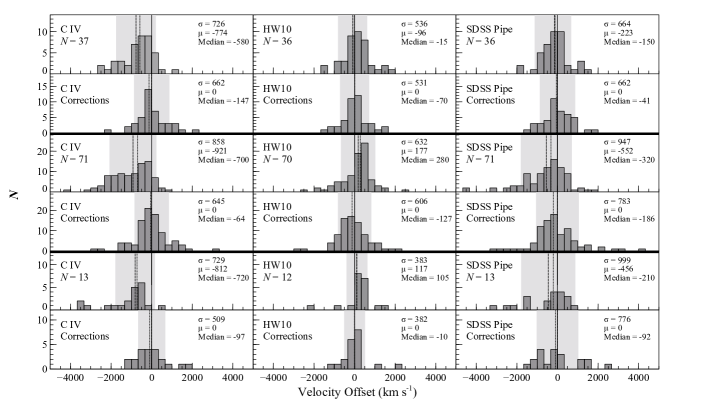
Figure 7: Same as Figure 4, but split into three redshift bins. Top six panels, middle six panels, and bottom six panels correspond to redshift Bin 1, Bin 2, and Bin 3, respectively, as described in the text.

Concerning the HW10-based method, our corrections produce improvements in standard deviation ranging from $\sim 1\%$ to $\sim 4\%$, with no apparent trend with redshift. Therefore, it seems that these improvements are not very sensitive to the coverage of the Mg ii line, which is absent from Bin 3. This result may be indicative of the overall robustness of the HW10 method, as found from the entire sample (see Section 3 and Figure 4). Mild improvements, and no significant redshift dependence, are observed for the SDSS Pipeline method, and the overall standard deviations of velocity offset distributions stemming from this method remain high ($\sim 780~{}\rm{km~{}s^{-1}}$) in Bins 2 and 3.

Table 7: Linear Regression Coefficients for Each Redshift Bin

UV-Based	Redshift	Regression	Value	Error	t-Value	Number of
Redshift Method	Bin	Coefficients				Sources
		$\alpha$	-1103	762	-1.45
	1	$\beta$	1022	436	2.35	37
		$\gamma$	37	60	0.62
		$\alpha$	-3382	561	-6.02
C iv	2	$\beta$	1357	441	3.08	71
		$\gamma$	204	48	4.21
		$\alpha$	-4802	1751	-2.74
	3	$\beta$	-994	1234	-0.81	13
		$\gamma$	391	167	2.34
		$\alpha$	-467	641	-0.73
	1	$\beta$	-29	359	-0.08	36
		$\gamma$	35	50	0.71
		$\alpha$	-758	532	-1.42
HW10	2	$\beta$	717	415	1.73	70
		$\gamma$	41	46	0.89
		$\alpha$	-27	1571	-0.02
	3	$\beta$	85	979	0.09	12
		$\gamma$	2	148	0.01
		$\alpha$	-251	780	-0.32
	1	$\beta$	149	440	0.34	36
		$\gamma$	10	61	0.17
		$\alpha$	-2661	681	-3.91
SDSS Pipe	2	$\beta$	1825	535	3.41	71
		$\gamma$	140	59	2.38
		$\alpha$	6314	2670	2.36
	3	$\beta$	4486	1881	2.38	13
		$\gamma$	-643	255	-2.52

In general, the greatest limitation in our ability to search for a redshift dependence is the disparity in the number of sources in each bin as is also portrayed by the large uncertainties on the regression coefficients in Table 7. Therefore, we derived the $\Delta v_{\rm corr}$ values in each redshift bin using the coefficients from Table 6, and found that the standard deviations on the distributions, when compared to those presented in Figure 7, are roughly consistent across all redshift bins (within $\sim 5\%$), which indicates no discernible redshift evolution in our sample. A significantly larger sample size, particularly in Bin 3 ($z\sim 3$), may allow for a more definitive conclusion in this matter. This highest redshift bin is particularly important given the absence of the Mg ii lines from the optical spectrum, and the need to reliably estimate redshifts of more distant sources.

In addition to exploring a possible redshift dependence, we also look to see if our ability to predict a quasar’s $z_{\rm sys}$ value depends on source luminosity. We trisect the calibration sample into three $L_{5100}$ ranges with roughly equal widths: $46.08-46.41$, $46.42-46.74$, and $46.75-47.09$, and look for any significant statistical deviations with respect to the entire sample. The results are shown in Figure 6. We find that there appears to be no clear dependence on source luminosity. A possible explanation for this result is that our sample is flux limited, and therefore it is difficult to disentangle the strong redshift-luminosity dependence.

4 Summary and Conclusions

We present an augmented catalog of spectroscopic properties obtained from NIR observations of a uniform, flux-limited sample of 260 SDSS quasars at $1.55\lesssim z\lesssim 3.50$. This catalog includes basic spectral properties of rest-frame optical emission lines, chiefly the Mg ii, H$\beta$, [O iii], Fe ii, and H$\alpha$ lines, depending on the availability of the line in the spectrum. These measurements provide an enhancement to the existing GNIRS-DQS database enabling one to more accurately analyze and investigate rest-frame UV-optical spectral properties for high-redshift, high-luminosity quasars in a manner consistent with studies of low-redshift quasars.

We also present prescriptions for correcting UV-based redshifts based on a subset of the GNIRS-DQS sample of 121 sources that are non-BAL, non-RL, have accurate C iv measurements, and have $z_{\rm sys}$ values obtained from prominent [O iii] measurements. We provide measurements of velocity offsets using three different UV-based methods compared to $z_{\rm sys}$ values. This 121-source sample is over twice the size of the calibration sample used in D20, and is both a higher quality and more uniform dataset than M17 and D20.

We attempt to correct for these velocity offsets using a linear regression based on UV continuum luminosity and C iv emission-line properties. Using this approach, we can decrease the standard deviation of the distribution of velocity offsets in our calibration sample by $\sim 2\%$ with respect to the best available UV-based redshift method, and by $\sim 18\%$ with respect to C iv-based redshifts. The SDSS Pipeline provides the least precise UV-based redshifts; in particular, the standard deviation of the corrected redshifts is still $\sim 20\%$ larger than those achieved for the other two methods. We find that the best way to obtain an accurate and precise $z_{\rm sys}$ value is using the C iv parameter space alone via four basic observables associated with the C iv emission line, and applying the following methodology:

1. Measure the observed peak wavelength, EW, and FWHM of C iv, and the monochromatic luminosity at 1350 Å ($L_{1350}$).

2. Calculate an initial redshift measurement, $z_{\rm meas}$, with the observed peak wavelength of C iv.

3. Use Equation 2 and the coefficients in Table 6 to calculate $\Delta v_{\rm corr}$.

4. Use Equation 3 with the observed $z_{\rm meas}$ and calculated $\Delta v_{\rm corr}$ to obtain a revised, more accurate, and more precise redshift measurement.

Additionally, we explore whether our prescriptions depend on 1) velocity width measurement, of which we determine there is no overt discrepancy based on methodology, 2) source redshift, where we determine that additional data are needed, particularly at the highest redshifts under investigation, in order to obtain more robust results, and 3) source luminosity, where no clear trends are apparent, consistent with the flux-limited nature of our sample.

A primary interest going forward would be bolstering the sample with supplementary observations of quasars, primarily at $z\sim 3$, in order to obtain statistically meaningful results on a potential redshift dependence, and further improve UV-based redshift determinations. It will also be interesting to test our prescriptions at the highest accessible redshifts, where considerably larger C iv blueshifts have been observed in sources at $z\gtrsim 6$, perhaps due to higher accretion rates (e.g., Meyer et al., 2019; Schindler et al., 2020; Ha et al., 2023). Another avenue of further investigation includes increasing the sample size of quasars with significantly higher spectral resolution, e.g., using Gemini’s Spectrograph and Camera for Observations of Rapid Phenomena in the Infrared and Optical (SCORPIO; Robberto et al., 2020), in order to further improve the UV-based redshift corrections by obtaining more accurate line peaks of spectral features. Machine learning can also play an important role as larger data sets will be produced that require redshift correction en masse. By utilizing the entire quasar UV spectrum, as opposed to a few key parameters, it will be possible to test if machine learning algorithms can produce more reliable estimates of $z_{\rm sys}$ much more efficiently than our prescriptions allow.

As future projects begin to produce data, we can expect that $\approx 10^{6}$ high-redshift ($z\gtrsim 0.8$) quasars will have redshifts determined through large spectroscopic surveys conducted in the rest-frame UV-optical regime from instruments such as the Dark Energy Spectroscopic Instrument (DESI; Levi et al., 2013; DESI Collaboration et al., 2016), the 4m Multi-Object Spectroscopic Telescope (de Jong et al., 2012), and the Subaru Prime Focus Spectrograph (PFS, Tamura et al., 2016). For those quasars at $1.5\lesssim z\lesssim 5.0$, coverage of the C iv emission line will enable crucial redshift corrections, as has been demonstrated in this work. Instruments such as the James Webb Space Telescope (JWST, Gardner et al., 2006) can provide simultaneous coverage of C iv, Mg ii, and [O iii], while other facilities can provide other systemic redshift indicators such as [C ii], CO, and Ly$\alpha$ halos (see, e.g., Decarli et al., 2018; Farina et al., 2019) for $6\lesssim z\lesssim 9$, allowing for similar investigations of redshift dependencies and corrections for the most distant known quasars.

Appendix A Comparing Different Velocity Widths of the C iv Line

In our regression analysis, we have elected to use the FWHM of the C iv line. However, there has been some debate in the literature concerning the overall reliability of using FWHM as the quantification of the velocity width of an emission line (e.g., Park et al., 2017; Dalla Bontà et al., 2020). While M17 and D20 used FWHM for their analyses, other methods for measuring velocity widths of emission-line profiles include Line Dispersion ($\sigma_{\rm line}$) and Mean Absolute Deviation (MAD) (e.g., Denney et al., 2016a; Dalla Bontà et al., 2020). We therefore repeated our analysis by replacing FWHM with each of these two velocity width methods, measured from the Gaussian fits presented in Table 4, and compared the results obtained from all three velocity widths. We find that replacing FWHM with $\sigma_{\rm line}$ or MAD gave no notable improvement in the dispersion on the relevant corrections, as shown in Figure 8. We thus have elected to adopt the FWHM parameterization throughout this work.

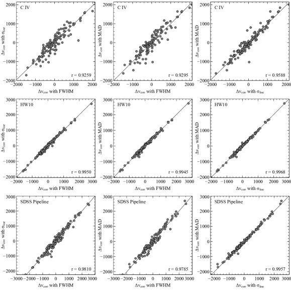
Figure 8: Comparison of the velocity offsets produced using C iv FWHM, $\sigma_{\rm line}$, and MAD for each UV-based redshift method. Each panel displays the correlation between the corrected velocity offset values produced by our regression analysis when using either FWHM, $\sigma_{\rm line}$, or MAD, along with a corresponding Pearson linear correlation coefficient $r$, where $r\rightarrow 1$ corresponds to a strong correlation. No significant difference exists in this regression analysis between the three different parameters.

References

- Alcock & Paczynski (1979) Alcock, C. & Paczynski, B. 1979, Nature, 281, 358. doi:10.1038/281358a0
- Baldwin (1977) Baldwin, J. A. 1977, ApJ, 214, 679. doi:10.1086/155294
- Begelman et al. (1991) Begelman, M., de Kool, M., & Sikora, M. 1991, ApJ, 382, 416. doi:10.1086/170731
- Bolton et al. (2012) Bolton, A. S., Schlegel, D. J., Aubourg, É., et al. 2012, AJ, 144, 144. doi:10.1088/0004-6256/144/5/144
- Boroson (2005) Boroson, T. 2005, AJ, 130, 381. doi:10.1086/431722
- Boroson & Green (1992) Boroson, T. A. & Green, R. F. 1992, ApJS, 80, 109. doi:10.1086/191661
- Carniani et al. (2018) Carniani, S., Maiolino, R., Marconi, A., et al. 2018, AGN13: Beauty and the Beast. The 13th Italian Meeting on Active Galactic Nuclei, 68
- Coatman et al. (2017) Coatman, L., Hewett, P. C., Banerji, M., et al. 2017, MNRAS, 465, 2120. doi:10.1093/mnras/stw2797
- Dalla Bontà et al. (2020) Dalla Bontà, E., Peterson, B. M., Bentz, M. C., et al. 2020, ApJ, 903, 112. doi:10.3847/1538-4357/abbc1c
- Dawson et al. (2013) Dawson, K. S., Schlegel, D. J., Ahn, C. P., et al. 2013, AJ, 145, 10. doi:10.1088/0004-6256/145/1/10
- de Jong et al. (2012) de Jong, R. S., Bellido-Tirado, O., Chiappini, C., et al. 2012, Proc. SPIE, 8446, 84460T
- Decarli et al. (2018) Decarli, R., Walter, F., Venemans, B. P., et al. 2018, ApJ, 854, 97. doi:10.3847/1538-4357/aaa5aa
- Denney et al. (2016a) Denney, K. D., Horne, K., Shen, Y., et al. 2016, ApJS, 224, 14. doi:10.3847/0067-0049/224/2/14
- Denney et al. (2016b) Denney, K. D., Horne, K., Brandt, W. N., et al. 2016, ApJ, 833, 33
- DESI Collaboration et al. (2016) DESI Collaboration, Aghamousa, A., Aguilar, J., et al. 2016, arXiv e-prints, arXiv:1611.00036
- Dix et al. (2020) Dix, C., Shemmer, O., Brotherton, M. S., et al. 2020, ApJ, 893, 14. doi:10.3847/1538-4357/ab77b6
- Paper II ((2023) Dix, C., Matthews, B. M., Shemmer, O., et al. 2023, ApJ, in press. arXiv:2304.02142
- Farina et al. (2019) Farina, E. P., Arrigoni-Battaia, F., Costa, T., et al. 2019, ApJ, 887, 196. doi:10.3847/1538-4357/ab5847
- Font-Ribera et al. (2013) Font-Ribera, A., Arnau, E., Miralda-Escudé, J., et al. 2013, J. Cosmology Astropart. Phys, 2013, 018. doi:10.1088/1475-7516/2013/05/018
- Gardner et al. (2006) Gardner, J. P., Mather, J. C., Clampin, M., et al. 2006, Space Sci. Rev., 123, 485. doi:10.1007/s11214-006-8315-7
- Gaskell (1982) Gaskell, C. M. 1982, ApJ, 263, 79
- Gibson et al. (2009) Gibson, R. R., Jiang, L., Brandt, W. N., et al. 2009, ApJ, 692, 758. doi:10.1088/0004-637X/692/1/758
- Ha et al. (2023) Ha, T., Dix, C., Matthews, B. M., Shemmer, O., et al. 2023, ApJ, in press. arXiv:2304.04783
- Hewett, & Wild (2010) Hewett, P. C., & Wild, V. 2010, MNRAS, 405, 2302
- Hogg (1999) Hogg, D. W. 1999, astro-ph/9905116
- Hopkins, & Elvis (2010) Hopkins, P. F., & Elvis, M. 2010, MNRAS, 401, 7
- Kellermann et al. (1989) Kellermann, K. I., Sramek, R., Schmidt, M., et al. 1989, AJ, 98, 1195
- Levi et al. (2013) Levi, M., Bebek, C., Beers, T., et al. 2013, arXiv:1308.0847
- Lyke et al. (2020) Lyke, B. W., Higley, A. N., McLane, J. N., et al. 2020, ApJS, 250, 8. doi:10.3847/1538-4365/aba623
- Maiolino et al. (2012) Maiolino, R., Gallerani, S., Neri, R., et al. 2012, MNRAS, 425, L66
- Mason et al. (2017) Mason, M., Brotherton, M. S., & Myers, A. 2017, MNRAS, 469, 4675. doi:10.1093/mnras/stx1080
- Matthews et al. (2021) Matthews, B. M., Shemmer, O., Dix, C., et al. 2021, ApJS, 252, 15. doi:10.3847/1538-4365/abc705
- McGreer et al. (2016) McGreer, I. D., Eftekharzadeh, S., Myers, A. D., et al. 2016, AJ, 151, 61. doi:10.3847/0004-6256/151/3/61
- Meyer et al. (2019) Meyer, R. A., Bosman, S. E. I., & Ellis, R. S. 2019, MNRAS, 487, 3305. doi:10.1093/mnras/stz1504
- Miller et al. (2011) Miller, B. P., Brandt, W. N., Schneider, D. P., et al. 2011, ApJ, 726, 20. doi:10.1088/0004-637X/726/1/20
- Murray et al. (1995) Murray, N., Chiang, J., Grossman, S. A., et al. 1995, ApJ, 451, 498. doi:10.1086/176238
- Nguyen et al. (2020) Nguyen, N. H., Lira, P., Trakhtenbrot, B., et al. 2020, ApJ, 895, 74. doi:10.3847/1538-4357/ab8bd3
- Pâris et al. (2017) Pâris, I., Petitjean, P., Ross, N. P., et al. 2017, A&A, 597, A79
- Pâris et al. (2018) Pâris, I., Petitjean, P., Aubourg, É., et al. 2018, A&A, 613, A51
- Park et al. (2017) Park, D., Barth, A. J., Woo, J.-H., et al. 2017, ApJ, 839, 93. doi:10.3847/1538-4357/aa6a53
- Rankine et al. (2020) Rankine, A. L., Hewett, P. C., Banerji, M., et al. 2020, MNRAS, 492, 4553. doi:10.1093/mnras/staa130
- Richards et al. (2011) Richards, G. T., Kruczek, N. E., Gallagher, S. C., et al. 2011, AJ, 141, 167. doi:10.1088/0004-6256/141/5/167
- Rivera et al. (2020) Rivera, A. B., Richards, G. T., Hewett, P. C., et al. 2020, ApJ, 899, 96. doi:10.3847/1538-4357/aba62c
- Robberto et al. (2020) Robberto, M., Roming, P. W. A., van der Horst, A. J., et al. 2020, Proc. SPIE, 11447, 1144774. doi:10.1117/12.2568031
- Runnoe et al. (2013) Runnoe, J. C., Ganguly, R., Brotherton, M. S., et al. 2013, MNRAS, 433, 1778. doi:10.1093/mnras/stt852
- Schindler et al. (2020) Schindler, J.-T., Farina, E. P., Bañados, E., et al. 2020, ApJ, 905, 51. doi:10.3847/1538-4357/abc2d7
- Shen et al. (2007) Shen, Y., Strauss, M. A., Oguri, M., et al. 2007, AJ, 133, 2222. doi:10.1086/513517
- Shen et al. (2008) Shen, Y., Greene, J. E., Strauss, M. A., et al. 2008, ApJ, 680, 169. doi:10.1086/587475
- Shen et al. (2011) Shen, Y., Richards, G. T., Strauss, M. A., et al. 2011, ApJS, 194, 45
- Shen et al. (2016) Shen, Y., Brandt, W. N., Richards, G. T., et al. 2016, ApJ, 831, 7
- Schneider et al. (2010) Schneider, D. P., Richards, G. T., Hall, P. B., et al. 2010, AJ, 139, 2360. doi:10.1088/0004-6256/139/6/2360
- Sheskin (2007) Sheskin, D. J. 2007, Handbook of Parametric and Nonparametric Statistical Procedures, (4th ed.; Chapman & Hall/CRC)
- Spergel et al. (2007) Spergel, D. N., Bean, R., Doré, O., et al. 2007, ApJS, 170, 377. doi:10.1086/513700
- Sulentic et al. (2000) Sulentic, J. W., Zwitter, T., Marziani, P., et al. 2000, ApJ, 536, L5. doi:10.1086/312717
- Sulentic et al. (2007) Sulentic, J. W., Bachev, R., Marziani, P., et al. 2007, ApJ, 666, 757. doi:10.1086/519916
- Tamura et al. (2016) Tamura, N., Takato, N., Shimono, A., et al. 2016, Proc. SPIE, 9908, 99081M. doi:10.1117/12.2232103
- Tytler & Fan (1992) Tytler, D. & Fan, X.-M. 1992, ApJS, 79, 1. doi:10.1086/191642
- Vanden Berk et al. (2001) Vanden Berk, D. E., Richards, G. T., Bauer, A., et al. 2001, AJ, 122, 549. doi:10.1086/321167
- Vietri et al. (2018) Vietri, G., Piconcelli, E., Bischetti, M., et al. 2018, A&A, 617, A81. doi:10.1051/0004-6361/201732335
- York et al. (2000) York, D. G., Adelman, J., Anderson, J. E., et al. 2000, AJ, 120, 1579
- Zhao et al. (2019) Zhao, G.-B., Wang, Y., Saito, S., et al. 2019, MNRAS, 482, 3497. doi:10.1093/mnras/sty2845