Adaptive Scheduling for Edge-Assisted DNN Serving

Abstract

Deep neural networks (DNNs) have been widely used in various video analytic tasks. These tasks demand real-time responses. Due to the limited processing power on mobile devices, a common way to support such real-time analytics is to offload the processing to an edge server. This paper examines how to speed up the edge server DNN processing for multiple clients. In particular, we observe batching multiple DNN requests significantly speeds up the processing time. Based on this observation, we first design a novel scheduling algorithm to exploit the batching benefits of all requests that run the same DNN. This is compelling since there are only a handful of DNNs and many requests tend to use the same DNN. Our algorithms are general and can support different objectives, such as minimizing the completion time or maximizing the on-time ratio. We then extend our algorithm to handle requests that use different DNNs with or without shared layers. Finally, we develop a collaborative approach to further improve performance by adaptively processing some of the requests or portions of the requests locally at the clients. This is especially useful when the network and/or server is congested. Our implementation shows the effectiveness of our approach under different request distributions (e.g., Poisson, Pareto, and Constant inter-arrivals).

1 Introduction

Motivation: Deep neural networks (DNNs) are widely used in many applications, including autonomous driving, cognitive assistance, cashierless stores, video surveillance and AR/VR. Many applications demand real-time inference. Existing works speed up DNN inference in two ways. One way is to train simpler models Iandola et al. (2016) to reduce computation overhead or use compressed DNNs (e.g.,  Han et al. (2015); Liu et al. (2018)). While significant progress has been made in this front (e.g., MobileNet Howard et al. (2017); Sandler et al. (2018) and ShuffleNet Ma et al. (2018); Zhang et al. (2018)), depending on the model complexity and learning tasks Chen et al. (2018); Wang et al. (2020); Zhang et al. (2019a), it is not always feasible to achieve real-time guarantees on the mobile devices. A complementary way for the mobile systems is to offload expensive DNN execution to edge servers (e.g., Ran et al. (2018); Liu et al. (2019)). Edge server is often preferred due to lower network latency. Collaborative DNN Kang et al. (2017a); Hu et al. (2019a) leverages the client’s computation resources to further reduce processing time. How to efficiently serve many requests on a server and support collaborative DNN execution poses an interesting system challenge. This is especially so for edge servers with limited memory and computational resources. Thus, we explore how to enable an edge server to efficiently serve many clients. This capability has significant implication on the viability of many mobile applications, including autonomous driving, smart homes, surveillance, as it is common for multiple mobile devices to share one edge server to run DNNs for their specific analytic tasks.

Opportunities and challenges: A natural way to serve multiple inference requests (e.g., coming from different cameras in the setting of video surveillance or autonomous driving) is to run requests in FIFO. Batching these requests together significantly enhances efficiency due to coalesced memory access (e.g., each weight in a DNN is loaded to the cache only once and used for all input data rather than loaded for each input data separately Inference ; Hu et al. (2018)).

Our measurement on a server with an Nvidia Tesla P100 GPU shows it takes around $24$ ms for GoogleNet Szegedy et al. (2015) to process one request, and 132 ms to process 10 requests one by one. In comparison, it takes only $28$ ms to process 10 requests as a batch, which is only slightly higher than running one request.

It is necessary to have a high enough request rate to create a batch. This is quite common since video analytic tasks require high frame rate for good accuracy and coverage. For example, video surveillance requires 15 frames/second (FPS) Honovich on each camera and many cameras are deployed across the environment. A typical experimental automated-driving vehicle consists of ten or more cameras monitoring different fields of view, orientations, and near/far ranges. Each camera generates a stream of images at 10-40 FPS depending on its function Yang et al. (2019). Moreover, an edge server can serve requests from different users, organizations, or vehicles, which further increases the request rates. These requests go through one or more DNNs, and some of these DNNs can be shared.

While batching benefit has been widely recognized, there is limited work on how to design schedulers to exploit batching benefits in DNN processing. Batching in DNN processing is different from general job batching because the latter batches either entire jobs or nothing, while DNN jobs go through well-defined layers and batching can take place in one or more layers (i.e., partial batching). Scheduling DNN jobs can make a big difference on the batching opportunities, hence the performance.

Designing batch-aware scheduling algorithms is challenging. Simply batching all or a fixed number of jobs is not always desirable since it requires earlier requests to wait to form a large batch and the batching benefit may vary significantly with the job arrival rate and the type of DNN layers. This motivates us to develop scheduling algorithms to support various performance objectives.

Our approach: We first develop a novel scheduling algorithm for requests using the same DNN. This is motivated by the observation that the same video analytics task typically uses the same DNN. For example, image classification uses GoogleNet Szegedy et al. (2015), object detection uses SSD Liu et al. (2016), and image segmentation uses FCN Long et al. (2015). We first consider there is no memory constraint and we can batch an arbitrary number of requests. We develop a dynamic programming algorithm to minimize the completion time for a given set of requests. Next, we consider the memory constraint, which limits the number of requests to batch. We further incorporate the deadline requirement for each request and maximize the on-time ratio of the jobs while taking advantage of batching benefits.

We further generalize our algorithm to handle requests that do not run the same DNN. In particular, we consider two scenarios: (i) requests that use different DNNs without shared layers and (ii) requests that go through multiple DNNs and some of these DNNs are shared. Both scenarios are common. For example, some clients may run image classification using ResNet He et al. (2016a) while other clients may run image segmentation using FCN Long et al. (2015). This falls into (i). A common scenario for (ii) arises when requests go through multiple DNNs and some of these DNNs are shared. For example, video prediction and segmentation (e.g., SDCNet Reda et al. (2018) and RTA Huang et al. (2018)) share the same optical flow DNN model but use different DNNs for the remaining processing. In this case, the requests at the optical flow DNN can be batched together. Similarly, human pose estimation usually consists of multi-person detection using a shared model (e.g., Faster RCNN Ren et al. (2015)) and predicting each person’s pose using different models (e.g., IEF Carreira et al. (2016) and G-RMI Papandreou et al. (2017)). Therefore, the requests at the object detection DNN can be batched together. We design scheduling algorithms for both (i) and (ii). We extend our scheduling algorithm to support DNNs with different numbers of shared layers.

Finally, we consider that a client can process some or portions of the requests to further reduce the request completion time. We develop two offloading algorithms that take into account network delay along with server and client processing time to adaptively determine whether to offload and how much to offload. Our client-side optimization is inspired by Kang et al. (2017a) but differs in that we consider the server’s batching benefit to maximize the efficiency.

We implement our approach on an edge server with an Nvidia Tesla P100 GPU and $16$GB GPU memory. We implement a client on the Nvidia Jetson Nano with a 128-core Maxwell GPU and 4 GB memory, which has been widely used as a client platform (e.g., Hu et al. (2019b); Hadidi et al. (2019)). Video frame transmissions are generated using WiFi and LTE packet traces.

Our main contributions are as follows:

• We design a batching-aware DNN scheduling algorithm to efficiently serve requests running the same DNN. It is flexible to support different objectives (e.g., minimize completion time or maximize on-time ratio). Our schemes significantly reduce the completion time and improve the system capacity (i.e., the maximum number of concurrent serving requests) by $20\%$-$67\%$ over Batch and by $40\%$-$400\%$ over No-Batch when serving a single DNN. When maximizing the on-time ratio, our scheme improves the system capacity by more than $22$% over the Earliest Deadline First (EDF) with batching strategy.

• We extend our algorithm to support multiple DNNs with different numbers of shared layers. Our scheme improves the system capacity by  more than $200\%$ and $50\%$ over No-Batch and Batch respectively.

• We enable collaborative DNN execution at the client side to speed up processing. The client can process some requests or portions of requests locally to reduce the server load. We show collaborative execution further improves the system capacity by more than $67\%$ over our optimized server only strategy.

• We implement our approaches on commodity hardware to demonstrate their effectiveness. We will release our code and data upon publication.

2 Related Work

Speeding up client-side DNN execution: One way to speed up DNN inference is to train simpler DNNs (e.g., MobileNet Howard et al. (2017); Sandler et al. (2018), SqueezeNet Iandola et al. (2016), ShuffleNet Ma et al. (2018); Zhang et al. (2018)) or compress DNNs Lane et al. (2016); Wu et al. (2016). Despite significant advances, several important learning tasks cannot run on mobile devices in real time (e.g., semantic segmentation, activity recognition, super-resolution video reconstruction). DeepMon Huynh et al. (2017) and DeepCache Xu et al. (2018) reuse pre-cached intermediate DNN output to avoid redundant computation for same input. NestDNN Fang et al. (2018) adaptively prunes filters from convolutional layers to reduce the computation demand when the available resource is insufficient. These approaches speed up DNN execution at the cost of degrading accuracy. Deepeye Mathur et al. (2017) and uLayer Kim et al. (2019) speed up DNN execution by using both CPU and GPU. We mainly focus on exploiting batching benefits in GPU.

Adjusting DNN configurations: The computational cost of DNNs depends on the input data size (e.g., the resolution and frame rate of the input video for video analytics tasks). Existing approaches, such as Deepdecision Ran et al. (2018), DARE Liu and Han (2018), Chameleon Jiang et al. (2018a)), optimize latency by adaptively adjusting the video resolution and frame rate according to the network condition and server workload. These approaches speed up the processing but reduce the accuracy. It also needs an accurate model that captures the relationship between the accuracy and computational cost, which is challenging.

Collaborative DNN execution: Collaborative processing leverages the client’s computation resources to further reduce processing time. Instead of offloading all computation, several works (e.g., Kang et al. (2017a); Hu et al. (2019a)) partition DNN processing between the client and server. Partitioning has to be done carefully since intermediate results tend to be larger than the input data. Our work complements the existing work by developing batching-aware collaborative processing to exploit batching benefits.

Batching user requests: Abadi et al. (2016); Hu et al. (2018); Shen et al. (2019); Kang et al. (2017b); Choi et al. (2021); Gujarati et al. (2020) batch DNN inferences to improve completion time. Nexus Shen et al. (2019) develops a scheduling algorithm to batch entire jobs using a new bin packing algorithm. Our work advances state-of-the-art as follows: (i) it introduces layer-wise batching-aware scheduling to create more batching opportunities in a single DNN, (ii) it enables batching for multiple DNNs with shared layers, and (iii) it optimizes different performance objectives (e.g., latency and on-time ratio). In Sec. 6, we show our system reduces the completion time by 25-32% over Nexus when running SDCNet and RTA. We explicitly optimize completion time or the number of tardy jobs for layer-wise batch-aware scheduling whereas LazyBatching Choi et al. (2021) blindly batches requests as long as they do not violate SLA, however batching may not always improve performance and should be used strategically. Clockwork Gujarati et al. (2020) does not consider layer-wise batching, which results in a much lower batching opportunity than ours. Mainstream Jiang et al. (2018b) and MCDNN Han et al. (2016) re-train the existing DNNs so that they have some layers in common. Requests can go through those common layers in batches to reduce processing delay. In comparison, we do not modify the DNNs and use scheduling to increase the batching opportunities.

Scheduling: There are several dynamic programming based scheduling algorithms (e.g., Brucker et al. (1998); Potts and Kovalyov (2000)). Different from the existing works, which treat each request as a single process, we develop scheduling algorithms for DNNs where each request involves multiple layers and our scheduler determines the order of requests and their corresponding layers to process. Moreover, the existing work (e.g., Brucker et al. (1998)) assumes batching requests does not have overhead. Batching DNN requests at different layers incurs overhead since a larger batch takes longer to process despite the batching benefit and requests at later layers also need to wait for the requests at earlier layers. Tang et al. (2019); Crankshaw et al. (2017); Fang et al. (2017) batch only requests arriving at the same time and improve hardware resource utilization across multiple GPUs. Our work supports more fine-grained layer-wise batching. Least Laxity Zhang et al. (2007) assigns a priority to a job based on its running time, but the job’s actual running time may be different if batched with other jobs. In comparison, we use the running time under batching for scheduling, which is more accurate.

Summary: Our work complements the existing work by developing batching-aware scheduling algorithms for DNNs to support different objectives (e.g., completion time and on-time ratio) and different usage scenarios (e.g., single DNN, multiple DNNs with or without shared layers, and collaborative DNN processing).

3 Motivation

Video analytics has real-time processing requirements. For example, object tracking needs to track objects at $30$ frames per second (FPS)  Chen et al. (2015). With recent advances (e.g., Liu et al. (2019); Apicharttrisorn et al. (2019)), the frame rate reduces to below $10$fps with marginal degradation in accuracy. Even with a reduced frame rate, it remains challenging to complete DNN processing exclusively on mobile devices due to limited computation resource.

DNN Completion Time: We measure the completion time of DNNs on the mobile device Nvidia Jetson Nano by executing each DNN on $100$ test images randomly selected from IMAGENET Deng et al. (2009). The completion time of a DNN is the average processing time of $100$ images. Table 1 shows the completion time for popular DNNs for different video analytics tasks. We use the optimized platform TensorRT to run those models. We set the mobile device to the low-power 5W mode and run DNNs with Float32 precision. It shows we can run those models only below $5$ FPS, which is consistent to the numbers in existing work Hadidi et al. (2019); Hanhirova et al. (2018); Zhang et al. (2019b).

Table 1: DNN completion time on Jetson Nano.

Model	VGG16	FCN	SSD
Task	Classification	Segmentation	Tracking
# Layers	38	40	51
Delay	230ms	240ms	270ms

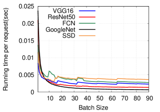
(a) Batching benefit.

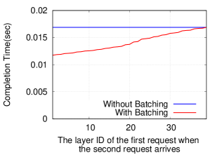
(b) Batching policy.

Figure 1: Batching Requests.

Batching benefits: DNN execution involves many memory operations. Processing requests in a batch can reduce the completion time by coalescing memory accesses Inference ; Hu et al. (2018). Fig. 1(a) shows that the completion time per batch reduces with the batch size for different DNNs. Batching $10$ requests reduces the running time per request by $63\%$, $81\%$, $57\%$, $88\%$ and $67\%$ for VGG16, ResNet50, FCN, GoogleNet and SSD, respectively. ResNet50 and GoogleNet have more batching benefits than other DNNs because they have more convolutional layers, which involve many memory operations and batching can reduce the memory accesses. Further increasing batch size from $10$ to $20$ reduces the per-request running time by $12\%$, $33\%$, $33\%$, $43\%$ and $14\%$ for VGG16, ResNet50, FCN, GoogleNet and SSD, respectively. When the batch size is already large, the benefit of batching more requests tapers off. In addition, the processing time per request does not always monotonically decrease with the batch size. For example, we observe an increase in completion time per request when increasing the batch size from $10$ to $11$ in FCN or increasing batch size from $17$ to $18$ in VGG. We use PyTorch to run DNNs in our experiments. PyTorch exploits cuDNN cudnn to run low-level computation for DNNs. cuDNN adapts the implementation algorithms (e.g., convolution operations) to trade off between the delay and memory utilization when the batch size changes cuDNN Convolution . The completion time changes when cuDNN changes the algorithm.

Impact on scheduling: Batching is only possible if requests are at the same layer. If we batch two requests at different layers, the earlier request might wait for the later request, which could incur overhead. Fig. 1(b) shows the completion time when two requests arrive at different time. We measure the completion time when running two requests for VGG16. The X-axis is the ID of the layer where the first request lies. If we do not batch them, the result remains the same. When the second request arrives when the first request has already finished many layers, the completion time is close to no batching. When the first request has not run beyond $20$ layers, batching the $2$ requests reduces the completion time by over 20%. Therefore, it is important to determine when and how to batch requests.

Shared layers in DNNs: Many DNNs share identical layers because it is challenging and time-consuming to design effective DNNs from scratch. Therefore, researchers often reuse existing DNN structures that have demonstrated good performance when designing new DNNs. For example, video prediction and segmentation (e.g., SDCNet Reda et al. (2018) and RTA Huang et al. (2018)) share the same optical flow DNN model but use different DNNs for the remaining processing. Similarly, human pose estimation usually consists of multi-person detection using a shared model (e.g., Faster RCNN Ren et al. (2015)) and predicting each person’s pose using different models (e.g., IEF Carreira et al. (2016) and G-RMI Papandreou et al. (2017)). In the above cases, there are batching opportunities for the shared layers.

Summary: Our results show that DNN execution on mobile devices is too slow to satisfy the real-time requirements. Batching can significantly reduce the completion time. It is possible to batch requests using the same DNN or different DNNs that share some layers. Batching requests coming at different time may incur significant overhead. The optimal batching policy should consider both batching benefits and overhead.

4 Our Approach

In this section, we first formulate the scheduling problem to minimize the completion time of a single DNN and present our dynamic programming algorithm (Sec. 4.1). We then consider how to maximize the job on-time ratio (Sec. 4.2). We further generalize to multiple DNNs with or without shared layers (Sec. 4.3). Finally, we extend it to support collaborative DNN execution, where clients can process portions of the DNN requests locally (Sec. 4.4).

4.1 Completion Time of One DNN

We develop a scheduling algorithm to optimize the completion time of a given set of requests. When a batch of requests finishes running a layer and new requests arrive, we re-compute the schedule for the updated set of requests. A unique aspect of batching-aware DNN scheduling is that requests are processed according to the DNN layer structure and can be batched with other requests only at the same layer.

4.1.1 Problem Formulation

Let $N$ denote the number of layers in a DNN, $R$ denote the set of requests in the system, $a_{i}$ denote the $i$-th request’s arrival time, $c_{i}$ denote the $i$-th request’s completion time. Any active request stays in GPU memory till it completes. Our goal is to minimize the total completion time.

Let $l_{i}$ denote the layer at which the request $i$ currently resides. $l_{i}=1$ indicates the request $i$ is waiting to run the first layer. Let $h_{k}(b)$ denote the running time of layer $k$ for a batch size $b$. Let $B$ denote the upper bound of the batch size at a layer due to limited GPU memory. We assume $h_{k}(b)$ has the following property: $h_{k}(b_{1}+b_{2})\leq h_{k}(b_{1})+h_{k}(b_{2})$ when $b_{1}+b_{2}\leq B$. $h_{k}(b)=+\infty$ if the batch size $b>B$. In our system with 16 GB GPU memory, $B=90$ is sufficient for even the largest model: SSD. We estimate $B$ by pre-allocating memory based on the maximum number of requests across all DNN layers. This estimation is conservative since different layers may have different number of requests. Dynamically adjusting memory bound for different layers can reduce memory requirement, but incurs considerable overhead due to frequent memory reallocation across layers. So we leave it to the future work.

4.1.2 Scheduling Algorithm

First, we consider the case without the batch size bound.

Unbounded Batch Size: We derive the following property for the optimal schedule using the FIFO scheduling (i.e., the job arriving first finishes first though not necessarily first served due to batching). For example, we can serve the second arriving request and then batch with the first request so both requests finish together.

Lemma 1

For a set of requests $R$ without the batch size bound, if we schedule a request to run, it will run till completion before running another request that arrives later assuming FIFO scheduling.

Proof sketch: If we schedule a request, it will be better to run this request till completion before running others. Switching to running other requests before finishing processing the ongoing requests that have already started causes all requests to have a longer processing time. Refer to pro for our proof.

Based on the above Lemma, we have the following policy when there is no limit on the batch size. If we schedule a request to run, it will batch all the requests that arrive earlier. This policy has several advantages. First, it ensures earlier requests will finish no later than later requests, which improves fairness and avoids starvation. Second, we can develop a dynamic programming algorithm to minimize the completion time. The dynamic programming algorithm picks a few splitting points, divides a request sequence into segments based on those points, and runs the requests segment by segment. Note that the segment means a sequence of requests batched together before running till the end. The segments run in the order of their arrival time (i.e., the segment involving the requests that arrive earlier is executed earlier). Within each segment, the latest requests are processed first and batched together with the earlier requests when they meet at the same layer. Each segment runs without stopping in the middle according to the Lemma 1.

For example, as shown in Figure 2, there are requests $A$, $B$, $C$, $D$, $E$ in the system. We split them into two segments: segment 1 involving requests A and B, and segment 2 involving requests C, D, and E. We first run segment 2, where request C runs from layer $l_{3}$ to layer $l_{4}$ alone, then batched with request D and runs till layer $l_{5}$, where it is batched further with request E and runs till the end. Then we run segment 1, where request A runs alone from layer $l_{1}$ to layer $l_{2}$, and is batched together with request B and runs till the end.

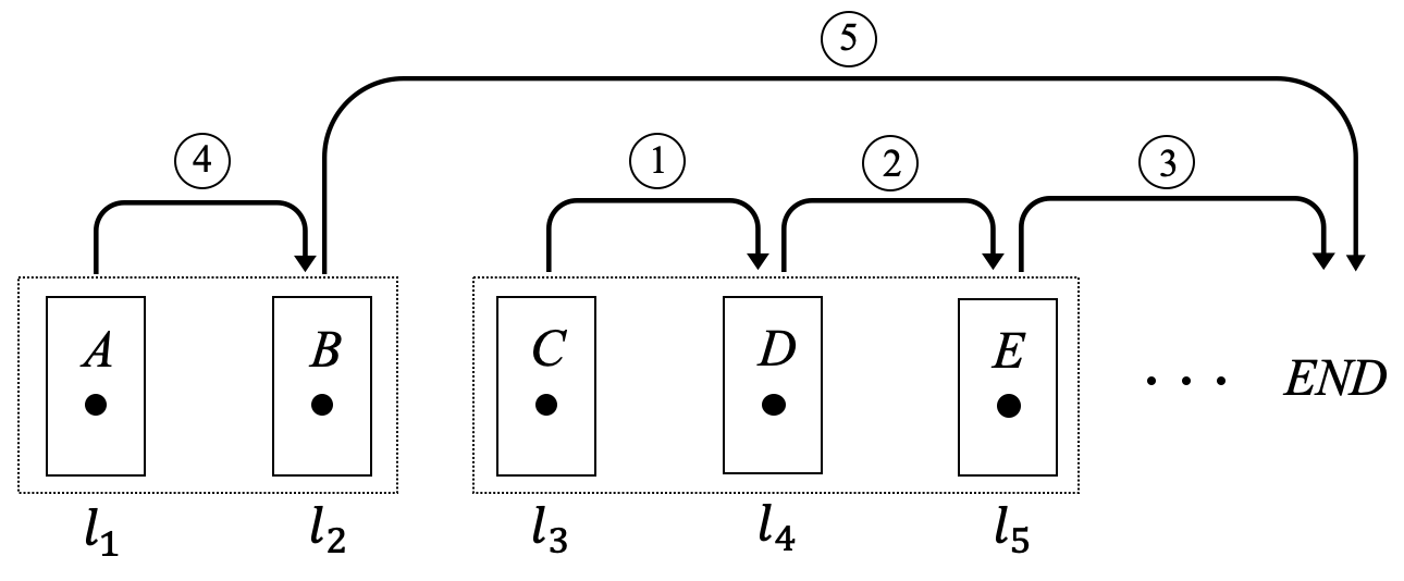
Figure 2: An example of request segments.

Dynamic programming: As we can see from the above example, how to split requests into multiple segments has significant impact on the performance. Our dynamic programming algorithm selects the splitting points to minimize the completion time. We sort the requests in an increasing order of their arrival time such that the arrival time of requests $j$ and $i$, denoted as $a_{j}$ and $a_{i}$ respectively, satisfies $a_{j}\leq a_{i}$ for any $j\leq i$. Since we process requests in the FIFO manner, we have $l_{j}\geq l_{i}$. Let $min\_cost(i)$ denote the minimum cost of running all requests from $i$ to $1$ under all possible ways of splitting, and $cost(i,j)$ denote the cost of running request $i$ and batched with all requests from $i$ to $j$ along the way till completion without splitting. $cost(i,j)$ can be computed by summing up the running time of each layer starting from layer $l_{i}$ weighted by $active(j)$, the number of active jobs before request $j$ finishes including those that finish together with request $j$. That is,

$$cost(i,j)=active(j)\times\sum_{k=l_{i}..N}{h_{k}(count(i,l_{i}))}\vspace*{-0.05in}$$ (1)

where $l_{i}$ is the layer at which request $i$ resides, and $count(i,l)$ denotes the number of requests that the request $i$ is batched together till it reaches the layer $l$ including the request $i$ and the existing requests at the layer $l$. The reason behind Equation 1 is that all jobs finishing together with request $j$ need to wait till they all finish. This includes running time from layer $l_{i}$ till layer $N$, where the cost of running a layer depends on the number of requests at the layer. $min\_cost(i)$ can be recursively computed as follows.

$$min\_cost(i)=min_{j=1..i}{(min\_cost(j-1)+cost(i,j))}\vspace*{-0.05in}$$ (2)

Intuitively, to compute the minimum cost of running requests $i$ through $1$ till completion, we search for the best splitting point $j$ where the requests from $i$ to $j$ run together in one segment and incurs $cost(i,j)$, and the cost of running requests from $1$ to $j-1$ is computed recursively by considering all possible ways of splitting.

Based on Equation 2, we implement a dynamic programming algorithm that computes a table of size $|R|$, where the $i$-th entry stores $min\_cost(i)$. We sort all requests in terms of their arrival, where request 1 arrives the earliest. We initialize $min\_cost(0)=0$ and set $min\_cost(1)$ to the cost of running request $1$ by itself till completion. Then we add $min\_cost(2)$ that computes $min(min\_cost(1)+cost(2,2),min\_cost(0)+cost(2,1))$, which considers running the request 1 by itself and then the request 2 versus batching the request 2 with the request 1. Similarly, we compute $min\_cost(3)$ as the minimum of $min\_cost(2)+cost(3,3)$, $min\_cost(1)+cost(3,2)$ and $min\_cost(0)+cost(3,1))$, which is the minimum of running the first two requests using all possible splittings and then running request 3 by itself, running the first request by itself and batching the requests 2 and 3, and batching the requests 1, 2, 3. As we can see, computing one table entry incurs $O(|R|)$ cost and there are $O(|R|)$ entries. So the overall time complexity is $O(|R|^{2})$.

We can prove the following theorem.

Theorem 1

Our dynamic programming algorithm minimizes completion time for requests using the same DNN among all FIFO schedules when there is no memory bound.

Proof: The property of the optimal FIFO schedule proved in Lemma 1 indicates the request sequence is divided into segments and the segment having the earliest arriving request will run first. The remaining problem is how to find the splitting points for the segments. Our recursive search in dynamic programming enumerates all splitting points for FIFO schedules. Hence it yields the lowest completion time among all FIFO schedules. Our evaluation considers memory constraints, and our scheme may not be the optimal in this case but still performs well.

Speedup computation: The complexity of our dynamic programming is $O(|R|^{2})$. When the number of requests is large, the dynamic programming incurs substantial delay. To further speed it up, we treat all requests at the same layer as one unit: batching all or no requests from a given layer. This reduces the complexity to $O(N^{2})$, where $N$ is the number of layers. In practice, only the layers that currently have requests matter, which is even smaller.

We further speed up by clustering layers into fewer groups. Let $G$ denote the number of groups. This will reduce the complexity to $O(G^{2})$. In our evaluation, we divide the layers into 5 groups, where each group has close to 1/5 running time of the entire DNN. Our results show that clustering layers speeds up our dynamic programming algorithm with only small impact on the performance (e.g., clustering layers reduces running time from 13ms to 2ms when computing schedule for 500 requests while yielding similar performance).

Incremental update: The schedule is subject to change upon finishing processing one or more requests at a layer and the arrival of a new request. In this case, we run our scheduling algorithm on CPU in parallel to processing the DNN requests on GPU. If the earlier request that changes the layer moves from layer $l_{1}$ to layer $l_{2}$ since the last schedule update, we reuse the table entries after layer $l_{2}$ at the time of last computation and re-compute the remaining entries as well as adding a new entry $min\_cost(i)$ for the new request.

To ensure real-time computation of schedule, we consider up to the first 500 active requests in the system. These requests should also be the ones that occupy the last several layers. The remaining requests will be considered in the future round. The intuition is that the requests arriving late cannot be scheduled immediately since the system already has many requests to process. We can delay calculating the schedule for these requests till the system is close to run them. Scheduling 500 requests takes less than 2ms.

Bounded Batch Size: When the maximum batch size is bounded by $B$, we still apply the above dynamic algorithm to find a schedule. The only modification is to set $cost(i)$ to $+\infty$ if the number of requests between the request $i\in R$ and $j\in R$ is larger than the bound $B$ and we stop searching the splitting points whose cost are already $+\infty$.

4.2 Maximize On-Time Ratio of One DNN

So far, we focus on minimizing the completion time. Next we explore minimizing the number of jobs that miss their deadlines. (i.e., tardy jobs). We develop two algorithms.

Our first algorithm is based on Earliest Deadline First (EDF). EDF is an optimal scheduling algorithm that minimizes the number of tardy jobs on preemptive uniprocessors without batching. It sorts and serves all jobs in increasing order of their deadlines. Different from traditional scheduling problems, in our context we can batch the jobs to reduce running time. To harness batching benefits while satisfying the deadline, we develop the following modified EDF. We sort all jobs according to their deadlines. Then we pick the job from the head of the sorted list and add it to the current batch as long as all jobs being scheduled so far satisfy their deadlines. If not, we will go to the next job and add it to the batch if the deadline of all jobs in the batch is honored, and iterate till the end of the list. In this way, we honor the deadlines as much as we can while opportunistically batch more jobs.

With batching, the modified EDF is no longer optimal. Therefore we develop another algorithm based on the dynamic programming in Section 4. We make two modifications: (i) we change the objective to minimize the number of tardy jobs, and (ii) we drop the jobs that have already missed their deadline. The output schedule from our algorithm gives the estimated completion time of each ongoing job in the system, and we drop the jobs whose estimated completion time cannot meet their deadline. While Lemma 1 no longer holds when minimizing the number of tardy jobs, the resulting algorithm significantly out-performs the above modified EDF in our evaluation since it explicitly considers the impact of batching when checking if the jobs satisfy the deadline.

4.3 Schedule Multiple DNNs

Multiple DNNs without shared layers: First, we consider scheduling multiple DNNs that do not share layers. Suppose the requests span across $M$ DNNs. For each DNN, we use the dynamic programming to derive its schedule. Then we enumerate all permutations of DNNs and select the permutation of DNNs that yields the smallest completion time. Since there are only a small number of commonly used DNNs (i.e., $M$ is small), enumerating all permutations of DNNs is affordable. Here running a DNN means running all requests of that DNN till completion. In the DNN permutations, we only consider model-wise permutations – we run all requests of a DNN before we start scheduling requests for another DNN. Since we re-compute the optimal schedule whenever a batch of requests finishes running a layer and new requests arrive, the optimized permutation may change over time to take into account the new requests. The scheduling algorithm outputs the order of the requests to serve until existing requests execute a layer and a new request arrives, in which case the schedule is re-computed based on the latest input. Therefore, requests from different DNNs can be served in an interleaved manner.

Multiple DNNs with shared layers: Next we consider requests that go through multiple DNNs and some of them can be shared. For example, the video prediction and segmentation tasks both use FlowNet2 Ilg et al. (2017) to compute the inter-frame optical flow and then use SDCNet Reda et al. (2018) and RTA Huang et al. (2018), respectively, for the remaining processing. In this case, requests for these two different tasks can be batched at FlowNet2.

We follow the strategy similar to the above. We first compute the schedule for each individual DNN. When computing the completion time for the $m$-th DNN, we ensure all requests belonging to the $m$-th DNN should run till completion and these requests will be batched with any requests arriving earlier (including those belonging to the other DNNs at the shared layers) up to the bound $B$ to maximize the batching benefit. When multiple DNNs are loaded to the GPU memory, $B$ is set to the total GPU memory used by all DNNs. We then derive the completion time for different orders of running DNNs and select the permutation with the lowest completion time.

Incremental update: The schedule is subject to change upon (i) a batch of requests finishing running a layer and the arrival of a new request, or (ii) a request moving across the boundary between shared and non-shared layers. Whenever any such event occurs, we re-run our scheduling algorithm on CPU in parallel to DNN execution on GPU. As before, we reuse the previous table as much as possible. We first find the earliest request that changes the layer since the last schedule update. Say the request moves from layer $i_{1}$ to layer $i_{2}$. We re-use the table entries after layer $l_{2}$ at the time of last schedule update. Reusing table entries allows a quick update of decision (e.g., within 2ms for 500 requests).

4.4 Collaborative DNN Execution

The GPUs on mobile devices are generally less powerful than those at the server. Mobiles also adjust the GPU speed to save power. For example, the Nvidia Jetson Nano device can run VGG16 at $4$fps and $11$fps when it is at $5$W and $20$W mode. Despite slower processing speed than the server, it can be beneficial for the mobile devices to process some requests locally when the server is overloaded. We develop two collaborative DNN execution strategies: (i) binary offloading (i.e., a client either processes or offloads an entire request), and (ii) partial offloading (i.e., a client processes the first few layers and offload the rest to the server).

Binary offloading: If the mobile device can process the request locally within the deadline, it will run it locally. Otherwise, it compares the local vs. remote processing (including network delay) and picks the one with the lower delay so that the job can finish faster. Local processing time can be simply estimated using measurement. Our evaluation uses the average running time of the DNN across $100$ runs as the estimate. Remote processing time is the sum of the network delay and server processing time, where the network delay is estimated based on the transmission size and network throughput using exponential weighted moving average (EWMA) with a weight of 0.3 on a new delay sample and the server processing time is determined using the above dynamic programming algorithm.

Partial offloading: When a request is offloaded to the server, the server may still be occupied with serving ongoing jobs and the new request is waiting idle. To enhance efficiency, the client could start processing its request locally till the server becomes available and then offloads the remaining processing to the server. We call this as partial offloading and it can further reduce the server load by processing the first few layers.

We let the server estimate and inform the client how long it will take to finish the new and existing requests. This is easy to do since the client can perform one-time profiling of popular DNNs to estimate the processing time of various layers. One-time profiling has been widely used (e.g., Kang et al. (2017a)).

To transmit the intermediate results to the server, we should compress the output from the client after processing some layers so that it can be sent efficiently to the server. We observe that video compression is much faster than file compression schemes (e.g., gzip), owing to available hardware accelerators, so we use lossless image compression H.264. It takes 1.5ms to compress at the client and 0.6ms to decompress at the server. In order to use H.264, we quantize the intermediate output from the client to INT8, and feed the output to the server. Running quantization incurs considerable overhead, so we run quantized models at the client and server to remove the need of quantizing the input or output while speeding up DNN processing. Fortunately, running a quantized model yields little degradation in the accuracy Choukroun et al. (2019); Wu et al. (2020).

Even with compression, the intermediate data size for the first few layers (which can finish on the client without incurring large delay) is larger than the original image size. Therefore, when the server is powerful as in our evaluation, partial offloading is attractive only for fast networks, such as 5G. On the other hand, when the server is slow (e.g., IoT devices), partial offloading is useful even on a slow network as in Kang et al. (2017a). Our approach automatically makes offload decision based on the server, client, and network speed. Our binary offloading does not increase the transmission size, and works for both slow and fast networks.

Our offloading strategies can be extended to incorporate the client’s energy (e.g., a client considers local processing as an option only when its battery power exceeds a threshold. Otherwise, it always offloads to the server).

5 System Implementation

Next describe the implementation details of our system. Fig. 3 shows our high-level system architecture.

5.1 Server Implementation

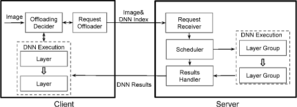
Figure 3: System architecture.

The server uses Pytorch Paszke et al. (2019) to run DNNs on the GPU Nvidia Tesla P100 Nvidia Tesla . It keeps track of requests at each layer and executes the scheduling algorithms implemented in Python. We revise the Pytorch DNN API so that Pytorch only runs a specified set of requests through specified layers. We use CUDA synchronization Cuda before we run a group so that GPU does not have any other active threads. We also use CUDA synchronization before we start running the next group so that all GPU threads for the existing group of layers have already completed. When we create a large batch, we also need to copy the input for each request to a continuous GPU memory block. The memory manager allocates a memory block when forming a batch and releases that block when the batch finishes running the next layer. Our scheduling algorithm requires the running time of each layer as the input. We profile the running time of each layer in various DNNs by varying the batch size. This is only a one-time profiling.

5.2 Collaborative DNN Execution

We implement our client on Nvidia Jetson Nano NVIDIA Jeston . Our system is not specific to this hardware and can run on any device (e.g., smartphones, IoT devices, etc). When mobile devices are not as powerful, they tend to offload all DNN tasks to the edge server. If they are more powerful (e.g., Nvidia Jetson Nano/TX2), they can process more requests locally. The client generates requests, which consist of images, arrival time, and the DNN to use. As described in Section 4.4, the client determines whether to offload the current request. If the request runs locally, the client runs some or all layers in the DNN using TensorRT Nvidia TensorRT , which is compatible with Pytorch. If the request requires complete offloading, the client will transmit the JPEG Wallace (1992) image and index of the DNN to the server via TCP. The server loads the DNN requested by the client to the memory, uses the JPEG library from OpenCV OpenCV to decompress the image, and feeds the decompressed data to the DNN as the input. If the request requires partial offloading, the client transmits intermediate results compressed by H.264 along with the next layer index in the DNN to the server, and the server decompresses using H.264 and finishes the remaining processing. The intermediate results consist of a sequence of feature maps, each of which is a gray-scale image. In both cases, upon finishing the DNN processing, the server uses the TCP to transmit results to the client.

6 Evaluation

6.1 Evaluation Methodology

DNN request traces: We generate DNN requests using a Poisson process by default. The average arrival rate is $10-350$ requests/sec. Each experiment runs $5000$ requests. We also try Pareto and deterministic inter-arrival time to understand the impact of different request arrival patterns.

Network traces: We use the packet traces Fouladi et al. (2018) collected from LTE uplink connections. Each one lasts for around $20$min. The throughput is in the range of $4$Mbps–$20$Mbps. We use this network traces to generate the reception timestamp of DNN requests at the server side. We only use transmission delay as the propagation delay to the edge server is negligible compared with the DNN processing time McLaughlin .

Image traces: We use video traces from the dataset MOT16 Milan et al. (2016). The images are resized to $240\times 240$, which is the input resolution of the pre-trained DNNs used in our experiments. Our system can run DNNs with any input resolution. The relative performance of different algorithms remains the same when the image resolution and GPU memory increase by the same amount. We use JPEG to compress images. The size of images varies from $0.12$Mbits to $0.33$Mbits.

DNNs: We evaluate popular DNNs for different analytics tasks: VGG16 Simonyan and Zisserman (2014), ResNet50 He et al. (2016b) and GoogleNet Szegedy et al. (2015) for classification, SSD Liu et al. (2016) for object detection, SDCNet Reda et al. (2018) for video prediction, and RTA Huang et al. (2018) and FCN Long et al. (2015) for video segmentation. We load all the models to the memory at the beginning, so there is no overhead of model loading when we switch DNNs when running multiple DNNs.

Performance metrics: We use three metrics: (i) completion time: the time duration from request generation to getting the DNN execution results at the client. The completion time captures the end-to-end latency of a request, which includes the latency of every step the request goes through in our system, including running the scheduling algorithm and performing memory copy. (ii) ratio of on-time requests: the ratio of requests that meet the user’s specified deadline, and (iii) capacity: the maximum request rate at which the on-time ratio is above 90%. We can easily see the system capacity from the on-time ratio graphs by looking for the load beyond which the on-time request ratio falls below 90%. The default deadline is 300ms and 150ms for evaluations with and without collaborative execution, respectively. We also vary the deadline to understand its impact.

Algorithms: We compare our scheduling algorithms with the following two baselines: (i) No-Batch, which runs all requests one by one, (ii) Batch, which sorts the requests in an increasing order of their arrival time and batches all requests starting from the first one up to the bound $B$. (iii) Our algorithms as described in Sec. 4. No-Batch runs on the unmodified version of PyTorch, while Batch and Our algorithms run on the modified version of PyTorch to support batching requests at different layers. Our modified PyTorch has little overhead: its Batch=1 version is equivalent to No-Batch and takes only 3ms longer.

Testbed: We develop a testbed to evaluate the performance of various algorithms. We generate requests from multiple clients using a single Linux machine based on real traces. We run DNN requests on the edge server in real time, which means that our results include all system overheads, including memory copying, thread switching and overheads related to monitoring and dynamically changing the PyTorch execution graph. For collaborative execution system, we use one real client to run all the client-side components on Nvidia Jetson Nano and send requests over WiFi. Requests from other clients are generated by a Linux machine according to the real traces collected from Nvidia Jetson Nano. All evaluation results are from our testbed.

6.2 Minimize One DNN Completion Time

6.2.1 Micro-Benchmark

Memory bound: We first conduct micro-benchmark to evaluate the impacts of memory bound. The server has limited memory, so it limits the batch size. We vary the memory bound from 50 to 90. 90 is the maximum batch size that the server can support given a limited memory.

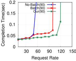
(a) Bound=90 (DNN: VGG16)

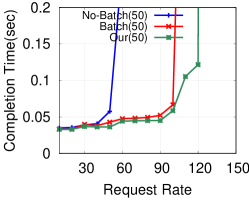
(b) Bound=50 (DNN: VGG16)

Figure 4: Performance for various memory bound.

Fig. 4 compares the completion time of different scheduling algorithms as we vary the batch size bound. As we would expect, our scheduling algorithm reduces the completion time significantly across all sizes. The reduction is $28\%$-$53\%$ over Batch and $62\%$ over No-Batch. Increasing the memory bound beyond $90$ does not affect our algorithm since we observe that it does not create batches over $90$ in our experiments. Decreasing the bound below $90$ limits the batching opportunities and increases the completion time. In comparison, No-Batch performs the same regardless of the maximum batch size as it always runs requests one by one. The Batch strategy uses a fixed batch size and does not work well since a too large batch size incurs a long waiting time to accumulate a large enough batch and a too small batch limits the batching opportunity.

Run-time Profiling: The actual run-time may not be exactly the same as offline profiling. Such estimation error is also present in our experiments when running on a real server. For example, we find the estimation error ranges between 1ms – 270ms in our evaluation when the batch size increases from 1 to 90. To evaluate the impacts of the estimation error, we collect traces of actual running time from the server. We evaluate the performance of our system using the VGG16 request traces and the collected running time traces. We find that the estimation error has little impact on the performance – the completion time based on the schedule calculated using the offline profiling vs. the actual running time differs by only around 12ms, within 10% of the average completion time. The schedule depends more on the relative ranking of the running time across different layers than the absolute running time, hence it is fairly robust to the estimation error.

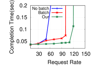
(a) VGG16

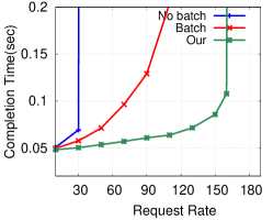
(b) ResNet50

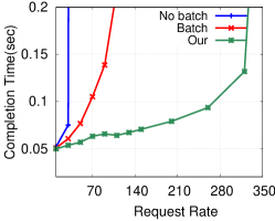
(c) GoogleNet

(d) FCN

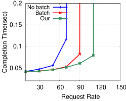
(e) SSD

Figure 5: Completion Time for a single DNN.

6.2.2 Performance Comparison

Next, we compare the performance of serving requests when running a single DNN in our system. We vary the request rate from $10$ to $150$ requests per second (req/sec). The request deadline is set to $150$ ms.

Fig. 5 shows our algorithm achieves the highest system capacity for all DNNs. The capacity of our algorithm is $120$, $160$, $320$, $70$ and $110$ for VGG16, ResNet50, GoogleNet, FCN and SSD, respectively. The corresponding numbers are $100$, $110$, $90$, $50$ and $90$ for the Batch strategy, and are $50$, $50$, $50$, $30$, $70$ for No-Batching. Our algorithm improves system capacity over Batch by $20\%$, $36\%$, $67\%$, $40\%$, $22\%$ for VGG16, ResNet50, GoogleNet, FCN and SSD, respectively; the corresponding improvement over No-Batch is $140\%$, $200\%$, $400\%$, $40\%$ and $57\%$. The system capacity improvement of our algorithm comes from strategically harnessing the batching benefits. ResNet50 and GoogleNet have more system capacity than the other DNNs due to more batching benefits in these DNNs.

Moreover, our scheduling algorithm not only improves capacity but also the completion time when the request load is below the capacity. It cuts down the completion time by up to $53\%$ over Batch when the request rate is below the capacity of the Batch strategy and by up to $29\%$ over the No-Batch strategy when the request rate is below the capacity of the No-Batch strategy. Our scheduling algorithm also improves the on-time ratio. The improvement is up to $69\%$ over Batch and $37\%$ over No-Batch.

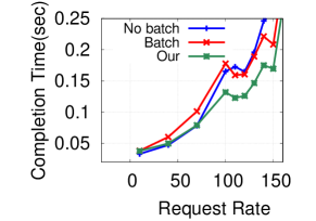
(a) Pareto

(b) Constant

Figure 6: VGG16 completion time for different request arrivals

6.2.3 Different Request Arrival Distributions

We evaluate the performance using different request inter-arrival distributions: Poisson, Pareto, and Constant since existing works (e.g., Downey ; Chabchoub et al. ) show Internet traffic exhibits Pareto distributions and video frames coming from a camera are likely to be constant inter-arrival. The inter-arrival time is $\lambda=[1/150,1/10]$ in Poisson distribution, $\alpha=1.25$ and $\kappa=\frac{(\alpha-1)}{\text{mean arrival rate}}$ in Pareto distribution, or a constant $\frac{1}{\text{mean arrival rate}}$ arrival. Fig. 5(a) and Fig. 6 compare the performance when serving VGG16. Our algorithm improves the capacity by $40\%$, $10\%$, and $30\%$ over No-Batch in Poisson, Pareto, and Deterministic inter-arrival, respectively. The improvement over Batch is $20\%$, $36\%$, and $20\%$, respectively.

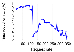
Figure 7: Comparison with Nexus for VGG16.

Comparison with Nexus: Fig. 7 compares our approach with Nexus Shen et al. (2019) using requests with a Deterministic inter-arrival time for VGG16. Our approach reduces the completion time over Nexus by 10.5% when the request rate is 95. Our benefit is even larger in multiple DNNs shown in Sec. 6.4.

6.3 Maximize On-Time Ratio

Next, we consider minimizing the number of tardy jobs. We compare the following three schemes: (i) EDF, (ii) Our-Time, our algorithm that minimizes completion time, (iii) Our-Tardy, our algorithm that maximizes the on-time ratio. We set the request deadline to $150$ms. All schemes drop jobs that have passed their deadline.

Fig. 8 shows the on-time ratio of these schemes are all close to 100% when the request rate is low; as the request rate increases, Our-Tardy yields the highest on-time ratio. For ResNet, the system capacity of EDF, Our-Time, and Our-Tardy is 80, 80 and 100. For VGG, the corresponding numbers are $90$, $100$ and $110$, respectively. Our-Tardy improves EDF by 22-25% and improves Our-Time by 10-22%. Our-Time can satisfy more requests’ deadline than EDF even though it does not explicitly consider the deadlines. This is because Our-Time minimizes the completion time, which indirectly reduces tardy jobs. EDF is less effective than Our-Time since it does not consider the batching benefit. Scheduling jobs only according to the order of the deadlines may reduce the batching opportunity, which results in higher running time and more tardy jobs.

We evaluate the on-time ratio by varying the deadline and request rates. The system capacity of Our-Tardy is 110 when the deadline is 150ms. Increasing deadline allows more requests to be served on time. All schemes have close to 100% on-time ratio when the request rate is 100 and the deadline is higher than 200ms. When the request rate is 120 and the deadline is higher than 200ms, both Our-Time and Our-Tardy improve EDF by around 50%. When the deadline is below 200ms, both Our-Time and Our-Tardy improve the on-time ratio by more than 20% over EDF. Therefore, our algorithm is effective in maximizing on-time ratio even if requests have different deadlines.

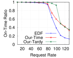
(a) ResNet

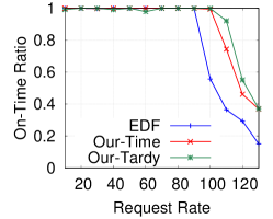
(b) VGG

Figure 8: Maximize on-time ratio for ResNet and VGG.

6.4 Performance for Multiple DNNs

DNNs without shared layers: Fig. 9(a) shows the performance when the requests are equally split between the two DNNs without shared layers. When serving ResNet50 and GoogleNet, the system capacity of No-Batch, Batch and our algorithm are $30$, $110$ and $190$, respectively. This is $500\%$ and $73\%$ improvement over No-Batch and Batch, respectively. We also run VGG16 and GoogleNet. The capacity of No-Batch, Batch and our algorithm are $50$, $90$ and $150$, respectively, which is $200\%$ and $67\%$ improvement over No-Batch and Batch, respectively. Our algorithm performs the best even for DNNs without shared layers by increasing batching opportunities in the same DNN.

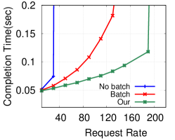
(a) 2 DNNs wo/ sharing (ResNet50, GoogleNet)

(b) 2 DNNs w/ shared layers (SDCNet, RTA)

Figure 9: 2 DNNs with and without shared layers.

If the request rate is below $110$, the average on-time ratios for Batch and our algorithm are $83\%$ and $96\%$, respectively, when serving ResNet50 and GoogleNet. We observe similar pattern when serving VGG16 and GoogleNet. Even if the request rate is within the system capacity of both our algorithm and Batch, our algorithm can still achieve higher on-time request ratio due to faster processing rate.

Skewed-splitting request distribution: We vary the request distribution across DNNs. Fig. 10 shows the performance when $25\%$ requests run ResNet50 and $75\%$ requests run GoogleNet. The system capacity are $30$, $90$ and $220$ for No-Batch, Batch and our algorithm, respectively. Compared with Fig. 9(a), the average completion time of our algorithm is $0.068$ sec under equal-splitting vs. $0.056$ sec under skewed-splitting when the request rate is 110. Moreover, the average on-time request ratio of our algorithm is $96\%$ and $98\%$ under equal-splitting and skewed-splitting, respectively. The skewed splitting between requests increases the batching benefits, thereby leading to larger improvement in all performance metrics.

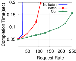
(a) Completion Time

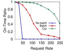
(b) On-Time Request Ratio

Figure 10: Performance for DNNs w/o shared layers having skewed-splitting distribution. (DNNs: ResNet50, GoogleNet; Request splitting: 1/4, 3/4)

DNNs with shared layers: Fig. 9(b) shows the performance when all requests go through the same optical flow model – FlowNet2 and then are equally split between SDCNet and RTA. The system capacity are $20$, $60$ and $90$ for No-Batch, Batch and our algorithm. So our approach yields $4.5\times$ and $1.5\times$ system capacity of No-Batch and Batch, respectively.

Since these two models are more time-consuming than others, we set the request deadline to 300ms for the evaluation. The average completion time is $0.232$sec and the average ratio of on-time requests is $98\%$ for our algorithm when the request rate is within the capacity. Without batching requests at the shared layers, the system capacity remains the same but the average completion time increases to $0.314$sec, which is $35\%$ higher than enabling batching at shared layers. Its on-time request ratio reduces to $42\%$. Thus, batching at the shared layers is beneficial.

We also evaluate the performance using skewed splitting, and observe skewed request distribution sees larger batching benefits and faster processing rate.

Comparison with Nexus Shen et al. (2019): We compare our approach with Nexus Shen et al. (2019) when the requests all go through FlowNet2 and then equally split between SDCNet and RTA. When the request rate is 70, Table 2 shows our approach reduces the completion time by 27%, 32%, 25% under Poisson, Pareto, and Constant inter-arrival time, respectively.

Table 2: Completion time (sec).

	Poisson	Pareto	Constant
Ours	0.124	0.157	0.109
Nexus	0.158	0.207	0.136

6.5 Collaborative DNN Execution

In our collaborative algorithm, a request is offloaded only when local execution is too slow to meet its deadline. The default deadline is $300$ms. The server runs the Our-Tardy to maximize the on-time ratio. In our experiments, all the client requests run either VGG16 or FCN. We vary the number of clients and each client generates requests according to a Poisson process with a mean arrival rate of $10$ req/sec. Among those clients, one client is running all the client-side components on Nvidia Jetson Nano and communicates with the server via WiFi, while the other clients are simulated to generate requests to the server.

Binary offloading: Fig. 11(a) shows the performance of VGG16 with binary offloading. The ratio of requests offloaded to server is $0.48$, $0.53$ and $0.60$ for No-Batch, Batch and our algorithm, respectively. Clients offload more requests in our scheme due to its faster server processing.

Our binary offloading runs requests locally as long as they can finish within the deadline. In this case, the completion time of the local requests may increase. For example, Fig. 11(a) shows that the completion time is around $0.125$ sec for VGG16 and $0.136$ sec for FCN, which is higher than the server processing time in Fig. 5(a) and Fig. 5(d). This is acceptable since the requests still finish in time and client processing saves network and server cost.

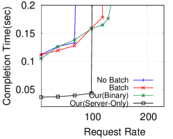
(a) Binary offloading

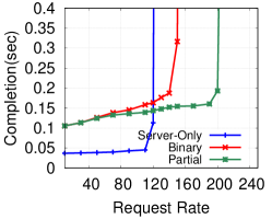
(b) Partial offloading

Figure 11: Collaborative execution for VGG16.

With binary offloading, the system capacity in VGG16 is $70$, $120$ and $140$ for No-Batch, Batch and our algorithm, respectively. The corresponding numbers are $30$, $50$ and $70$ for FCN. Binary offloading improves the system capacity of serving VGG16 by $25\%$ and $17\%$ for Batch and our algorithm, respectively. When serving FCN, the capacity improvement of Batch and our algorithm is $40\%$ and $29\%$, respectively. By running some requests locally on the client, our scheme has a higher capacity. No-Batch has the same capacity w/ and wo/ binary offloading for VGG16 because the client is not fast enough to reduce the server’s queue.

Partial offloading: The completion time includes client processing time, network transmission time, and server processing time. Due to the relatively large intermediate results, we multiply the throughput in the network traces by $10\times$ so that it is closer to that in the 5G networks. The client runs quantized DNN layers, uses H.264 to compress intermediate results, and transmits data over WiFi. Fig. 11(b) shows the performance of partial offloading when running VGG16. The binary offloading improves the system capacity from $120$ in the server-only scheme (Sec. 4.1) to $140$, and partial offloading further improves the capacity to $200$, which translates to 67% increase in the system capacity over the server-only scheme. For FCN, the binary offloading improves the system capacity from 70 to 90, and partial offloading further improves to 120, out-performing the server-only scheme by 71%, since the client can more often perform local processing.

6.6 Summary and Discussion

Summary: Our main findings are as follows: (i) Our algorithm improves system capacity up to $4\times$ and $67\%$ over No-Batch and Batch, respectively, when serving a single DNN. We observe more performance improvement for DNNs having more batching benefits. (ii) Our algorithm can efficiently exploit batching benefits for multiple DNNs with or without shared layers. For DNNs with shared layers, our algorithm achieves more performance improvement. We observe more than $200\%$ and $50\%$ improvements in the system capacity over No-Batch and Batch. (iii) Our algorithm is flexible to maximize the job on-time ratio. Compared with the EDF strategy, our algorithm can improve the system capacity by more than $22$%. (iv) Collaborative DNN execution further improves the system capacity of our algorithm by around $67\%$.

7 Conclusion

We develop batch-aware DNN scheduling for edge servers. It supports (i) different optimization objectives: minimizing completion time or maximizing job on-time ratio, (ii) requests using the same or different DNNs with or without shared layers, and (iii) collaborative DNN execution to further reduce processing delay by adaptively running some or portions of requests locally at the client side. Our extensive evaluation demonstrates its effectiveness.

References

- Iandola et al. [2016] Forrest N Iandola, Song Han, Matthew W Moskewicz, Khalid Ashraf, William J Dally, and Kurt Keutzer. Squeezenet: Alexnet-level accuracy with 50x fewer parameters and< 0.5 mb model size. arXiv preprint arXiv:1602.07360, 2016.
- Han et al. [2015] Song Han, Huizi Mao, and William J Dally. Deep compression: Compressing deep neural networks with pruning, trained quantization and huffman coding. arXiv preprint arXiv:1510.00149, 2015.
- Liu et al. [2018] Sicong Liu, Yingyan Lin, Zimu Zhou, Kaiming Nan, Hui Liu, and Junzhao Du. On-demand deep model compression for mobile devices: A usage-driven model selection framework. In MobiSys, pages 389–400. ACM, 2018.
- Howard et al. [2017] Andrew G Howard, Menglong Zhu, Bo Chen, Dmitry Kalenichenko, Weijun Wang, Tobias Weyand, Marco Andreetto, and Hartwig Adam. Mobilenets: Efficient convolutional neural networks for mobile vision applications. arXiv preprint arXiv:1704.04861, 2017.
- Sandler et al. [2018] Mark Sandler, Andrew Howard, Menglong Zhu, Andrey Zhmoginov, and Liang-Chieh Chen. Mobilenetv2: Inverted residuals and linear bottlenecks. In CVPR, pages 4510–4520, 2018.
- Ma et al. [2018] Ningning Ma, Xiangyu Zhang, Hai-Tao Zheng, and Jian Sun. Shufflenet v2: Practical guidelines for efficient cnn architecture design. In ECCV, pages 116–131, 2018.
- Zhang et al. [2018] Xiangyu Zhang, Xinyu Zhou, Mengxiao Lin, and Jian Sun. Shufflenet: An extremely efficient convolutional neural network for mobile devices. In CVPR, pages 6848–6856, 2018.
- Chen et al. [2018] Liang-Chieh Chen, Yukun Zhu, George Papandreou, Florian Schroff, and Hartwig Adam. Encoder-decoder with atrous separable convolution for semantic image segmentation. In ECCV, pages 801–818, 2018.
- Wang et al. [2020] Haicheng Wang, Vineeth Bhaskara, Alex Levinshtein, Stavros Tsogkas, and Allan Jepson. Efficient super-resolution using mobilenetv3. In Adrien Bartoli and Andrea Fusiello, editors, Computer Vision – ECCV 2020 Workshops, pages 87–102, Cham, 2020. Springer International Publishing. ISBN 978-3-030-67070-2.
- Zhang et al. [2019a] Chen-Lin Zhang, Xinxin Liu, and Jianxin Wu. Towards real-time action recognition on mobile devices using deep models. CoRR, abs/1906.07052, 2019a. URL http://arxiv.org/abs/1906.07052.
- Ran et al. [2018] Xukan Ran, Haolianz Chen, Xiaodan Zhu, Zhenming Liu, and Jiasi Chen. Deepdecision: A mobile deep learning framework for edge video analytics. In INFOCOM 2018, pages 1421–1429. IEEE, 2018.
- Liu et al. [2019] Luyang Liu, Hongyu Li, and Marco Gruteser. Edge assisted real-time object detection for mobile augmented reality. In MobiCom. ACM, 2019.
- Kang et al. [2017a] Yiping Kang, Johann Hauswald, Cao Gao, Austin Rovinski, Trevor Mudge, Jason Mars, and Lingjia Tang. Neurosurgeon: Collaborative intelligence between the cloud and mobile edge. In SIGARCH, volume 45, pages 615–629. ACM, 2017a.
- Hu et al. [2019a] Chuang Hu, Wei Bao, Dan Wang, and Fengming Liu. Dynamic adaptive dnn surgery for inference acceleration on the edge. In INFOCOM 2019, pages 1423–1431. IEEE, 2019a.
- [15] Inference. Inference: The next step in gpu-accelerated deep learning. https://devblogs.nvidia.com/inference-next-step-gpu-accelerated-deep-learning/.
- Hu et al. [2018] Yitao Hu, Swati Rallapalli, Bongjun Ko, and Ramesh Govindan. Olympian: Scheduling gpu usage in a deep neural network model serving system. In Proceedings of the 19th International Middleware Conference, pages 53–65. ACM, 2018.
- Szegedy et al. [2015] Christian Szegedy, Wei Liu, Yangqing Jia, Pierre Sermanet, Scott Reed, Dragomir Anguelov, Dumitru Erhan, Vincent Vanhoucke, and Andrew Rabinovich. Going deeper with convolutions. In CVPR, 2015. URL http://arxiv.org/abs/1409.4842.
- [18] John Honovich. Frame rate guide for video surveillance. https://ipvm.com/reports/frame-rate-surveillance-guide.
- Yang et al. [2019] Ming Yang, Shige Wang, Joshua Bakita, Thanh Vu, F. Donelson Smith, James H. Anderson, and Jan-Michael Frahm. Re-thinking cnn frameworks for time-sensitive autonomous-driving applications: Addressing an industrial challenge. In RTS, 2019.
- Liu et al. [2016] Wei Liu, Dragomir Anguelov, Dumitru Erhan, Christian Szegedy, Scott Reed, Cheng-Yang Fu, and Alexander C Berg. Ssd: Single shot multibox detector. In ECCV, pages 21–37. Springer, 2016.
- Long et al. [2015] Jonathan Long, Evan Shelhamer, and Trevor Darrell. Fully convolutional networks for semantic segmentation. In CVPR, pages 3431–3440, 2015.
- He et al. [2016a] Kaiming He, Xiangyu Zhang, Shaoqing Ren, and Jian Sun. Deep residual learning for image recognition. In CVPR, pages 770–778, 2016a.
- Reda et al. [2018] Fitsum A Reda, Guilin Liu, Kevin J Shih, Robert Kirby, Jon Barker, David Tarjan, Andrew Tao, and Bryan Catanzaro. Sdc-net: Video prediction using spatially-displaced convolution. In ECCV, pages 718–733, 2018.
- Huang et al. [2018] Po-Yu Huang, Wan-Ting Hsu, Chun-Yueh Chiu, Ting-Fan Wu, and Min Sun. Efficient uncertainty estimation for semantic segmentation in videos. In ECCV, pages 520–535, 2018.
- Ren et al. [2015] Shaoqing Ren, Kaiming He, Ross Girshick, and Jian Sun. Faster r-cnn: Towards real-time object detection with region proposal networks. In Neurips, pages 91–99, 2015.
- Carreira et al. [2016] Joao Carreira, Pulkit Agrawal, Katerina Fragkiadaki, and Jitendra Malik. Human pose estimation with iterative error feedback. In CVPR, pages 4733–4742, 2016.
- Papandreou et al. [2017] George Papandreou, Tyler Zhu, Nori Kanazawa, Alexander Toshev, Jonathan Tompson, Chris Bregler, and Kevin Murphy. Towards accurate multi-person pose estimation in the wild. In CVPR, pages 4903–4911, 2017.
- Hu et al. [2019b] Zhiming Hu, Ahmad Bisher Tarakji, Vishal Raheja, Caleb Phillips, Teng Wang, and Iqbal Mohomed. Deephome: Distributed inference with heterogeneous devices in the edge. In The 3rd International Workshop on Deep Learning for Mobile Systems and Applications, pages 13–18, 2019b.
- Hadidi et al. [2019] Ramyad Hadidi, Jiashen Cao, Yilun Xie, Bahar Asgari, Tushar Krishna, and Hyesoon Kim. Characterizing the deployment of deep neural networks on commercial edge devices. In IISWC, 2019.
- Lane et al. [2016] Nicholas D Lane, Sourav Bhattacharya, Petko Georgiev, Claudio Forlivesi, Lei Jiao, Lorena Qendro, and Fahim Kawsar. Deepx: A software accelerator for low-power deep learning inference on mobile devices. In IPSN, page 23. IEEE Press, 2016.
- Wu et al. [2016] Jiaxiang Wu, Cong Leng, Yuhang Wang, Qinghao Hu, and Jian Cheng. Quantized convolutional neural networks for mobile devices. In CVPR, pages 4820–4828, 2016.
- Huynh et al. [2017] Loc N Huynh, Youngki Lee, and Rajesh Krishna Balan. Deepmon: Mobile gpu-based deep learning framework for continuous vision applications. In MobiSys, pages 82–95. ACM, 2017.
- Xu et al. [2018] Mengwei Xu, Mengze Zhu, Yunxin Liu, Felix Xiaozhu Lin, and Xuanzhe Liu. Deepcache: principled cache for mobile deep vision. In MobiCom, pages 129–144. ACM, 2018.
- Fang et al. [2018] Biyi Fang, Xiao Zeng, and Mi Zhang. Nestdnn: Resource-aware multi-tenant on-device deep learning for continuous mobile vision. In MobiCom, pages 115–127. ACM, 2018.
- Mathur et al. [2017] Akhil Mathur, Nicholas D Lane, Sourav Bhattacharya, Aidan Boran, Claudio Forlivesi, and Fahim Kawsar. Deepeye: Resource efficient local execution of multiple deep vision models using wearable commodity hardware. In MobiSys, pages 68–81. ACM, 2017.
- Kim et al. [2019] Youngsok Kim, Joonsung Kim, Dongju Chae, Daehyun Kim, and Jangwoo Kim. layer: Low latency on-device inference using cooperative single-layer acceleration and processor-friendly quantization. In EuroSys, page 45. ACM, 2019.
- Liu and Han [2018] Qiang Liu and Tao Han. Dare: Dynamic adaptive mobile augmented reality with edge computing. In ICNP, pages 1–11. IEEE, 2018.
- Jiang et al. [2018a] Junchen Jiang, Ganesh Ananthanarayanan, Peter Bodik, Siddhartha Sen, and Ion Stoica. Chameleon: scalable adaptation of video analytics. In Sigcomm, pages 253–266. ACM, 2018a.
- Abadi et al. [2016] Martín Abadi, Paul Barham, Jianmin Chen, Zhifeng Chen, Andy Davis, Jeffrey Dean, Matthieu Devin, Sanjay Ghemawat, Geoffrey Irving, Michael Isard, et al. Tensorflow: A system for large-scale machine learning. In OSDI 16), pages 265–283, 2016.
- Shen et al. [2019] Haichen Shen, Lequn Chen, Yuchen Jin, Liangyu Zhao, Bingyu Kong, Matthai Philipose, Arvind Krishnamurthy, and Ravi Sundaram. Nexus: a gpu cluster engine for accelerating dnn-based video analysis. In SOSP, pages 322–337. ACM, 2019.
- Kang et al. [2017b] Daniel Kang, John Emmons, Firas Abuzaid, Peter Bailis, and Matei Zaharia. Noscope: optimizing neural network queries over video at scale. Proceedings of the VLDB Endowment, 10(11):1586–1597, 2017b.
- Choi et al. [2021] Yujeong Choi, Yunseong Kim, and Minsoo Rhu. Lazy batching: An sla-aware batching system for cloud machine learning inference. In HPCA, pages 493–506. IEEE, 2021.
- Gujarati et al. [2020] Arpan Gujarati, Reza Karimi, Safya Alzayat, Wei Hao, Antoine Kaufmann, Ymir Vigfusson, and Jonathan Mace. Serving DNNs like clockwork: Performance predictability from the bottom up. In OSDI 20, pages 443–462, 2020.
- Jiang et al. [2018b] Angela H Jiang, Daniel L-K Wong, Christopher Canel, Lilia Tang, Ishan Misra, Michael Kaminsky, Michael A Kozuch, Padmanabhan Pillai, David G Andersen, and Gregory R Ganger. Mainstream: Dynamic stem-sharing for multi-tenant video processing. In 2018 USENIX Annual Technical Conference (USENIXATC 18), pages 29–42, 2018b.
- Han et al. [2016] Seungyeop Han, Haichen Shen, Matthai Philipose, Sharad Agarwal, Alec Wolman, and Arvind Krishnamurthy. Mcdnn: An approximation-based execution framework for deep stream processing under resource constraints. In MobiSys, pages 123–136. ACM, 2016.
- Brucker et al. [1998] Peter Brucker, Andrei Gladky, Han Hoogeveen, Mikhail Y Kovalyov, Chris N Potts, Thomas Tautenhahn, and Steef L Van De Velde. Scheduling a batching machine. Journal of scheduling, 1(1):31–54, 1998.
- Potts and Kovalyov [2000] Chris N Potts and Mikhail Y Kovalyov. Scheduling with batching: A review. European journal of operational research, 120(2):228–249, 2000.
- Tang et al. [2019] Xuehai Tang, Peng Wang, Qiuyang Liu, Wang Wang, and Jizhong Han. Nanily: A qos-aware scheduling for dnn inference workload in clouds. In HPCC/SmartCity/DSS, pages 2395–2402. IEEE, 2019.
- Crankshaw et al. [2017] Daniel Crankshaw, Xin Wang, Guilio Zhou, Michael J Franklin, Joseph E Gonzalez, and Ion Stoica. Clipper: A low-latency online prediction serving system. In NSDI 17, pages 613–627, 2017.
- Fang et al. [2017] Zhou Fang, Tong Yu, Ole J Mengshoel, and Rajesh K Gupta. Qos-aware scheduling of heterogeneous servers for inference in deep neural networks. In CIKM, pages 2067–2070. ACM, 2017.
- Zhang et al. [2007] W. Zhang, S. Teng, Z. Zhu, X. Fu, and H. Zhu. An improved least-laxity-first scheduling algorithm of variable time slice for periodic tasks. In ICCI, pages 548–553, 2007. doi:10.1109/COGINF.2007.4341935.
- Chen et al. [2015] Tiffany Yu-Han Chen, Lenin Ravindranath, Shuo Deng, Paramvir Bahl, and Hari Balakrishnan. Glimpse: Continuous, real-time object recognition on mobile devices. In Sensys, pages 155–168. ACM, 2015.
- Apicharttrisorn et al. [2019] Kittipat Apicharttrisorn, Xukan Ran, Jiasi Chen, Srikanth V Krishnamurthy, and Amit K Roy-Chowdhury. Frugal following: Power thrifty object detection and tracking for mobile augmented reality. In Sensys, pages 96–109. ACM, 2019.
- Deng et al. [2009] Jia Deng, Wei Dong, Richard Socher, Li-Jia Li, Kai Li, and Li Fei-Fei. Imagenet: A large-scale hierarchical image database. In 2009 IEEE conference on computer vision and pattern recognition, pages 248–255. Ieee, 2009.
- Hanhirova et al. [2018] Jussi Hanhirova, Teemu Kämäräinen, Sipi Seppälä, Matti Siekkinen, Vesa Hirvisalo, and Antti Ylä-Jääski. Latency and throughput characterization of convolutional neural networks for mobile computer vision. In MMSys, pages 204–215, 2018.
- Zhang et al. [2019b] Daniel Zhang, Nathan Vance, Yang Zhang, Md Tahmid Rashid, and Dong Wang. Edgebatch: Towards ai-empowered optimal task batching in intelligent edge systems. In RTSS, pages 366–379. IEEE, 2019b.
- [57] cudnn. cuDNN developer guide. https://docs.nvidia.com/deeplearning/sdk/cudnn-developer-guide/index.html.
- [58] cuDNN Convolution. cudnn convolution functions. https://docs.nvidia.com/deeplearning/cudnn/developer-guide/index.html#tensor-ops-conv-functions.
- [59] https://osf.io/r7wsc/?view_only=0daed714f6264c32a2f039a2eff9bd6b.
- Ilg et al. [2017] Eddy Ilg, Nikolaus Mayer, Tonmoy Saikia, Margret Keuper, Alexey Dosovitskiy, and Thomas Brox. Flownet 2.0: Evolution of optical flow estimation with deep networks. In CVPR, pages 2462–2470, 2017.
- Choukroun et al. [2019] Yoni Choukroun, Eli Kravchik, Fan Yang, and Pavel Kisilev. Low-bit quantization of neural networks for efficient inference. In ICCVW, pages 3009–3018. IEEE, 2019.
- Wu et al. [2020] Hao Wu, Patrick Judd, Xiaojie Zhang, Mikhail Isaev, and Paulius Micikevicius. Integer quantization for deep learning inference: Principles and empirical evaluation. arXiv preprint arXiv:2004.09602, 2020.
- Paszke et al. [2019] Adam Paszke, Sam Gross, Francisco Massa, Adam Lerer, James Bradbury, Gregory Chanan, Trevor Killeen, Zeming Lin, Natalia Gimelshein, Luca Antiga, et al. Pytorch: An imperative style, high-performance deep learning library. In Neurips, pages 8024–8035, 2019.
- [64] Nvidia Tesla. Nvidia tesla p100. https://www.nvidia.com/en-us/data-center/tesla-p100/.
- [65] Cuda. Cuda runtime API. https://docs.nvidia.com/cuda/cuda-runtime-api/group__CUDART__STREAM.html.
- [66] NVIDIA Jeston. Nvidia jeston nano developer kit. https://developer.nvidia.com/embedded/jetson-nano-developer-kit.
- [67] Nvidia TensorRT. Nvidia tensorrt. https://developer.nvidia.com/tensorrt.
- Wallace [1992] Gregory K Wallace. The jpeg still picture compression standard. IEEE transactions on consumer electronics, 38(1):xviii–xxxiv, 1992.
- [69] OpenCV. Opencv. https://opencv.org.
- Fouladi et al. [2018] Sadjad Fouladi, John Emmons, Emre Orbay, Catherine Wu, Riad S Wahby, and Keith Winstein. Salsify: low-latency network video through tighter integration between a video codec and a transport protocol. In NSDI 18, pages 267–282, 2018.
- [71] Ronan McLaughlin. 5g low latency requirements. https://broadbandlibrary.com/5g-low-latency-requirements/.
- Milan et al. [2016] Anton Milan, Laura Leal-Taixé, Ian Reid, Stefan Roth, and Konrad Schindler. Mot16: A benchmark for multi-object tracking. arXiv preprint arXiv:1603.00831, 2016.
- Simonyan and Zisserman [2014] Karen Simonyan and Andrew Zisserman. Very deep convolutional networks for large-scale image recognition. arXiv preprint arXiv:1409.1556, 2014.
- He et al. [2016b] Kaiming He, Xiangyu Zhang, Shaoqing Ren, and Jian Sun. Deep residual learning for image recognition. In CVPR, June 2016b.
- [75] Allen B. Downey. Lognormal and pareto distributions in the internet. https://www.allendowney.com/research/longtail/downey03lognormal.pdf.
- [76] Yousra Chabchoub, Christine Frickeer, Fabrice Guillemin, and Philippe Robert. On the statistical characterization of flows in internet traffic with application to sampling. https://arxiv.org/pdf/0902.1736.pdf.