Online Ensemble of Models for Optimal Predictive Performance with Applications to Sector Rotation Strategy

Abstract

• Asset-specific factors are commonly used to forecast financial returns and quantify asset-specific risk premia. Using various machine learning models, we demonstrate that the information contained in these factors leads to even larger economic gains in terms of forecasts of sector returns and the measurement of sector-specific risk premia. To capitalize on the strong predictive results of individual models for the performance of different sectors, we develop a novel online ensemble algorithm that learns to optimize predictive performance. The algorithm continuously adapts over time to determine the optimal combination of individual models by solely analyzing their most recent prediction performance. This makes it particularly suited for time series problems, rolling window backtesting procedures, and systems of potentially black-box models. We derive the optimal gain function, express the corresponding regret bounds in terms of the out-of-sample $R$-squared measure, and derive optimal learning rate for the algorithm. Empirically, the new ensemble outperforms both individual machine learning models and their simple averages in providing better measurements of sector risk premia. Moreover, it allows for performance attribution of different factors across various sectors, without conditioning on a specific model. Finally, by utilizing monthly predictions from our ensemble, we develop a sector rotation strategy that significantly outperforms the market. The strategy remains robust against various financial factors, periods of financial distress, and conservative transaction costs. Notably, the strategy’s efficacy persists over time, exhibiting consistent improvement throughout an extended backtesting period and yielding substantial profits during the economic turbulence of the COVID-19 pandemic.

Keywords: Ensemble of Models; Machine Learning; Multiplicative Weights Update Method; Online Learning; Risk Premium; Sector Rotation.

1 Introduction

The utilization of machine learning (ML) methods in quantitative finance has garnered significant interest in recent years, primarily due to their flexibility in modeling, potential for improved forecasting performance, scalability, and ability to automate numerous research processes in big data problems. With a vast range of ML models available and an increasing number of financial factors purported to explain stock return variations, the market of forming new predictive relations has grown exponentially. Nonetheless, as emphasized by Albuquerque et al., (2022), numerous ML models experience significant instabilities, as they are designed to minimize prediction error through structured risk minimization (see Vapnik, , 2000). Consequently, there has been an increasing demand for novel ensemble techniques that combine individual models.

The combination of ML models to produce a meta-prediction represents a crucial step towards enhancing forecasting performance because it combines information captured by individual models from potentially different subsets of predictors and averages their individual instabilities. To this end, Wood et al., (2023) have presented a theoretical framework for ensemble diversity that extends beyond the conventional bias-variance trade-off, incorporating an additional component of diversity across models. Similarly, Vogklis and Nasios, (2022) have attributed the success of their forecasting model in the M5 Forecasting Competition to the diversity of ML models and their ensemble. Notably, building ensembles of models has become a significant industry-wide effort, with many of the largest technology companies working on model ensembles, as detailed in Weill et al., (2019) and Sawyers, (2021).

We introduce a novel online ensemble algorithm that improves sequentially the weights of the individual models based on their past forecasting performance. This algorithm is model-agnostic and relies solely on the most recent forecasting performance of individual models, allowing for privacy preservation in cases where the construction of the individual models or the data used in the training cannot be disclosed, and only the forecasted values can be shared with the ensemble learning algorithm. This approach facilitates the use of models developed separately by multiple groups within an organization or those being constructed within a web-scale social network of autonomous micromanagers. Examples of the latter include micropredictions, which are repeated, short-term forecasts (i.e., nowcasts) based on real-time data streams. As described in Cotton, (2022), micropredictions are important in numerous domains, including stock markets, energy consumption, and weather forecasting.

The ability to update ensemble weights online also offers adaptivity in dynamic environments, where the optimal ensemble may shift over time due to changes in the predicted signals’ underlying structures or modifications to individual models. These changes may not be easily traceable and may preclude the possibility of backtesting with offline ensemble algorithms.

Another appealing characteristic of our ensemble algorithm is that it is particularly suitable for performing time series predictions using a rolling window backtesting method, which is a widely employed out-of-sample evaluation technique in time-series analysis and quantitative finance. In case the data is drawn from a random sample the optimal ensemble models can be created using cross-validation, bagging, or boosting methods. However, these methods suffer from computational inefficiencies and are hindered in the context of time-series data by serial correlation or potential non-stationarities—see the discussion in Albuquerque et al., (2022). In contrast, our ensemble algorithm updates its weights optimally and in real-time, based on the previous performance of the individual models, which is executed through the Multiplicative Weights Update Method (MWUM). The MWUM has been applied in diverse fields such as machine learning (AdaBoost, Winnow, Hedge Alabdulmohsin, , 2018), optimization (solving linear programs Plotkin et al., , 1995), theoretical computer science (devising a fast algorithm for linear programming and semidefinite programming Arora et al., , 2005), and game theory (Bailey and Piliouras, , 2018). In this study, the MWUM is utilized in a novel context of learning the optimal weights for ensemble model averaging in a recurring forecasting task. The MWUM is suitable for this task due to its gradient-free nature and fixed updating rule, which ensures that any poorly performing model is assigned a weight that exponentially decreases over consecutive forecasts, faster than the linear gains from exploring different models. Consequently, as demonstrated below, the resulting linear combination of forecasts achieves effective regret bounds that can evaluated using past data to access the convergence to the optimal ensemble.

In addition to the new application of the MWUM method for ensemble learning. This paper makes several theoretical contributions. Firstly, we develop an optimal for this task gain function from the MWUM that effectively balances the trade-off between exploration and exploitation, and it allows us to learn an ensemble with the highest out-of-sample $R$-squared ($R^{2}_{oos}$). Secondly, we derive the optimal learning rate for the online algorithm. This rate ensures that the ensemble algorithm converges quickly and accurately without any tuning parameters. Finally, we present new regret bounds expressed using the aforementioned $R^{2}_{oos}$. This statistical forecasting evaluation and model selection measure is widely used in statistics and we show that our ensemble algorithm converges to the optimal ensemble with the highest $R^{2}_{oos}$, and we provide regret bounds to measure the algorithm’s performance.

The out-of-sample $R$-squared is often used in asset pricing as a measure of risk premium, see Gu et al., (2020), and Leippold et al., (2022), where the former paper compares various ML methods for predicting individual stock returns in the US market, while the latter finds strong predictive results in the Chinese stock market using similar ML techniques. Our MWUM algorithm’s cost function is thus related to measuring risk premia. Weigand, (2019) provides a theoretical overview of recent academic studies in empirical asset pricing that employ ML techniques; see also Karolyi and Van Nieuwerburgh, (2020) and references therein for an overview of recent advances of ML in finance. Ndikum, (2020) explores the performance of ML algorithms and techniques that can be used for financial asset price forecasting. They make comparisons between the modern ML algorithms and the traditional Capital Asset Pricing Model (CAPM) on US equities. Nard et al., (2020) expand the study of Gu et al., (2020) by proposing a new method based on variable subsample aggregation of model predictions for equity returns using a large-dimensional set of factors. They aggregate predictions from different models using relative $R^{2}_{oos}$. In another work, Chen et al., (2023) combine three different deep neural network structures in a novel way (i.e., a feedforward network, a recurrent Long Short-Term Memory network, and a generative adversarial network) to estimate an asset pricing model using fundamental no-arbitrage condition as criterion function. Our paper contributes to this emerging literature on applications of ML methods in asset pricing. It provides a comparative analysis of ML methods for measuring risk premia of sector returns, gives new insights into performance attribution in terms of predictability of different factors for different sectors, and it demonstrates large economic gains from using ML for sector forecasting that are much greater than those documented on the level of individual stocks by the aforementioned authors.

Sector rotation strategies often rely on economic marketwide indicators such as monetary policy, interest rates forecasts, and commodity prices to construct a portfolio that shifts between sectors. In a recent paper Karatas and Hirsa, (2021) use sector-specific macro indicators to create a two-stage deep learning based sector rotation strategy with profitable out-of-sample performance. In this study, we go a step further by leveraging stock-specific factors that are commonly used in the literature to explain individual stock returns. We aggregate the information from these factors to the sector levels and construct sector-level features for different (non-) linear ML models. Our strategy aligns with the Arbitrage Pricing Theory (APT), which asserts that asset-specific factors can explain the returns of individual stocks. However, unlike standard APT modeling, we do not necessarily impose a linear relation between the aggregated factors and sector returns. Instead, we use the proposed sector-level factors as features in different ML algorithms to predict future sector returns. The use of ML models allows us to exploit that information content better than standard linear regression models. Aggregating factors to the sector level and focusing on the predictability of sector returns also improves the signal-to-noise ratio in the data. The result is that we generate more accurate predictions for each ML model considered and further improve them by aggregating predictions using our online ensemble learning algorithm. Empirically, we show that our ensemble of ML models which are trained on our sector-specific factors leads to a high-performing sector rotation strategy that is not arbitraged out over time, and is highly profitable during the recent COVID-19 period.

The remainder of the paper is structured as follows. Section 2 outlines our methodology for aggregating the data to the sector level and measuring sector performance. In Section 3 we describe the ensemble algorithm and its theoretical properties. Section 4 presents our empirical analysis, including prediction performance of different ML models for different sectors, performance attribution of individual factors in each sector, the performance of the sector rotation strategy, and robustness analysis. Section 5 summarizes our results and concludes the paper. The appendix includes all the proofs, and provides supplementary information, including details on probabilistic principal component analysis, the ML models used for predictions, the factors used in the analysis, and the SIC Codes used to form sector returns.

2 Modeling Sector Returns

We break down the assets into industry levels based on the first two digits of Standard Industrial Classification (SIC) codes (see Appendix for the sector definitions and their SIC codes) and then present the data in a two- and three-dimensional layout—time and sector, and time, sector, and factor, respectively.

Consider $N$ sectors and denote the excess return of sector $i$ over one period from $t$ to $t+1$ by $r_{i,t+1}$, where $i=1,\dots,N$ and $t=1,\dots,T$. We use two different methods to calculate sector returns. The first one is an equally-weighted return, i.e., we calculate the mean of the returns across all the companies that are part of a given sector in a given time period. Since large-cap stocks in a given sector are usually the leaders of the given industry and sector, and they represent well-known, established companies, the second version of sector returns is capitalization-weighted, i.e., we compute a weighted average of the returns with the weights equal to the ratio of the average company capitalization relative to the total average capitalization of the sector. The two forms of sector returns can be expressed as following

$$r_{i,t+1}=\begin{cases}\frac{1}{n_{i}}\sum_{j=1}^{n_{i}}r_{i,t+1}^{j}\;&\text{equally-weighted }\\ \frac{\sum_{j=1}^{n_{i}}c_{i,t}^{j}r_{i,t+1}^{j}}{\sum_{j=1}^{n_{i}}c_{i,t}^{j}}\;&\text{capital-weighted}\\ \end{cases}$$ (1)

where $r_{i,t+1}^{j}$ is the return value for company $j$ which belongs to sector $i$ in time $t+1$, $c_{i,t}^{j}$ is the corresponding market cap of that company on day $t$, and $n_{i}$ is the total number of the companies in the sector $i$.

In its most general form, we describe a sector (excess) returns $r_{i,t+1}$ as an additive prediction error model:

$$r_{i,t+1}=E_{t}(r_{i,t+1})+\epsilon_{i,t+1},$$ (2)

where

$$E_{t}(r_{i,t+1})=g(z_{i,t}),$$ (3)

where $z_{i,t}$ is a $P$-dimensional vector of sector level factors. We assume the conditional expectation $g(z_{i,t})$ is a function of predictor variables, and $\epsilon_{i,t+1}$ is an independent and identically distributed random noise. The predictors are lagged relative to $r_{i,t+1}$, so we can construct predictive models for next-period returns.

The function $g(\cdot)$ can be either a simple linear or an arbitrary nonlinear function. We focus on a sector-specific functional form of $g(\cdot)$, i.e., only information regarding companies in a given sector can predict the returns of that sector. Regarding different models that we consider to estimate the function $g(\cdot)$, we have 13 machine learning models along with three simple linear models. We include ordinary least squares (OLS) regression, principal component regression (PCR), least absolute shrinkage and selection operator (LASSO), gradient-boosted regression trees (GBRT), and neural networks with one to twelve layers (NN1-NN12). The definitions of all the models are given in the Appendix.

The dependent variables $z_{i,t}$ in all the models are the aggregated sector-level factors. We have information on individual companies’ level in terms of $94$ different factors also used in Gu et al., (2020) (see the Appendix for the list of all the factors and the references where they were introduced) for $9000$ companies from $60$ different sectors. We need to group the factor variables into sectors and aggregate them to predict sector returns. Including all the factors for all the assets as the predictors would lead on average to $14100(=9000*94/60)$ predictors per sector. In order to avoid such a large feature space and to extract the most important information from the individual assets, we apply the principal component analysis, which reduces the dimensionality of the predictors. In particular, we define the sector-level factors $z_{i,t}$ as the first principal components of a given asset-specific characteristic for assets in a given sector. The first principal component, by its definition, explains the most variation in a given matrix of factors. Intuitively, $z_{i,t}$ is a univariate representation of the given factor for all the assets in a given sector that is the best univariate characteristic of the original asset-specific factors. In Section 4.2, we evaluate these factors in terms of their predictive performance for each sector.

Since many of the factors exhibit missing data, we estimate the principal components using probabilistic principal component analysis (PPCA). Classical PCA developed by Hotelling, (1933) and Hotelling, (1936) requires complete matrix of the data. The PPCA introduced by Tipping and Bishop, (1999) combines PCA with an Expectation-Maximization (EM) algorithm from Dempster et al., (1977), i.e., it is a maximum likelihood estimator of the principal components that can also accommodate missing values in the input data. We describe the details of the PPCA method in the Appendix.

To assess predictive performance for sector excess return forecasts, we calculate the $R^{2}_{oos}$ for each sector, $i=1\ldots,N$, and $\tau$ number of rolling windows

$$R_{oos}^{2}(\tau)=1-{\frac{\sum_{t=1}^{\tau}(r_{i,t}-\widehat{r}_{i,t})^{2}}{\sum_{t=1}^{\tau}r_{i,t}^{2}}},$$ (4)

where $r_{i,t}$ and $\widehat{r}_{i,t}$ are the $i$th sector returns over the next period, and the one-step-ahead predictions of the $i$th sector returns over the next period, respectively, for two different types of sector returns defined in (1).

The evaluation is only assessed on the testing sample using a rolling window exercise. The denominator is the sum of squared excess returns without demeaning. Gu et al., (2020) argue that the sample mean is a poor estimator of the expected return, and it is better to use in the denominator zero as the predictor of the expected returns. Note that because the sector returns are computed as (weighted) averages of individual asset returns, the values of our sector $R^{2}_{oos}$ in (4) can be compared with the $R^{2}_{oos}$ computed from individual stock predictions that are given in Gu et al., (2020).

Our predictive models allow the investor to allocate capital between sectors. However, they cannot predict the returns of individual stocks and optimally allocate the capital to individual assets. Therefore, in portfolio performance analysis in Section 4.3, we select the best-performing sectors, and we fix the portfolio weights for the individual stocks from the selected sectors. The portfolio weights are fixed consistently with the definitions of the sector returns in (1). Since the individual asset weights in the portfolio strategy are the same as in the composition of the sector returns, we can use these sector returns in the performance evaluation of sector rotation strategies in Section 4 because they represent the returns of the corresponding feasible portfolio.

3 Performance Driven Ensemble of Models

Combining machine learning models to form a meta-prediction is an important step toward better forecasting performance. In our context, each of the machine learning algorithms discussed in the Appendix generates different predictions for each sector. As shown in Section 4.1 some models systematically underperform compared with other models in a given sector, but they have much better performance when used to predict the returns of a different sector. In order to benefit from this heterogeneity in performance across models and sectors, we propose a meta-strategy that provides a prediction of the returns of sector $i$, $\widetilde{r}_{i,t}$, for $t=1,\ldots,\tau$, where $\tau$ is the number of rolling windows, as $\widetilde{r}_{i,t}=(\widehat{r}^{(1)}_{i,t},\ldots,\widehat{r}^{(L)}_{i,t})^{\top}\mathbf{p}^{(t)}$, and $\mathbf{p}^{(t)}\in\mathbb{R}^{L}$ is a vector of nonnegative weights at rolling window forecast $t$, that sum up to one, i.e., $\mathbf{p}^{{(t)}^{\top}}\mathbbm{1}_{L}$, where $\mathbbm{1}_{L}=[1,\ldots,1]^{\top}\in\mathbb{R}^{L}$. The series of vectors $\mathbf{p}^{(t)}$, for $t=1,\ldots,\tau$ is obtained using the Multiplicative Weights Update Method, which instead of looking back at all the previous forecasting periods, it works online, and after each rolling window evaluates the performance of each model to gradually learn how to combine predictions from different models.

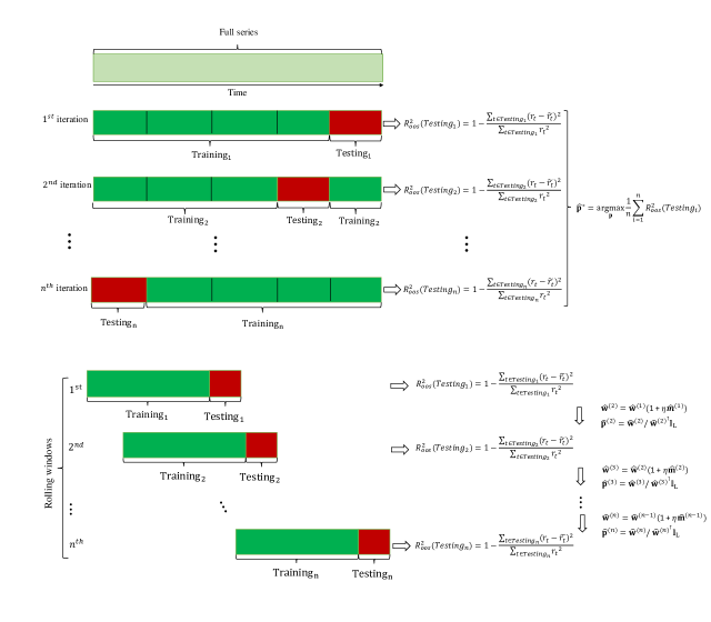
Figure 1: Comparison between standard CV (top panel) and the MWUM algorithm (bottom panel). The CV uses future observations to train a model. It is computationally intensive because it requires retraining of all the iterations whenever new data arrives. In the online algorithm, the meta-prediction is formed online on new data based on past forecasting performance. On the right in both panels are the corresponding optimizations for the meta-parameters $\mathbf{p}$. CV is usually done using a grid search over a finite set of meta-parameters or using some optimization routine over a compact set of meta-parameters. MWUM algorithm uses a multiplicative update rule with an optimal gain function $\widehat{\mathbf{m}}^{(\cdot)}$ and learning rate $\eta$. It does not require an unstable computation of the gradient of out-of-sample performance measure with respect to the meta-parameters, or any grid search; and it is performed online.

Figure 1 compares our rolling window approach with standard $n$-fold cross-validation algorithm. The cross-validation (CV) method is well suited for an $iid$ data because it uses future observations to train a model, and it requires the retraining of all the iterations whenever a new data arrives. Rolling window approach trains and tests the models sequentially on new data. CV is usually done using a grid search over some set of meta-parameters or some gradient-based optimization over the meta parameters space. Both approaches are very computationally intensive and cannot be done on large parameter space, such as ensemble weights for a large set of models. We propose a new optimal updating rule which is very fast in computations and does not require any gradient or grid search. It is done online so that when new data arrives, the parameters can be updated instantaneously, even in large dimensions. It is based on the MWUM algorithm, and as shown below it has good theoretical properties. The details of the algorithm are given below.

0:  $\left\{\widehat{\mathbf{r}}_{t}\right\}_{t=1,\ldots,T}$, where $\widehat{\mathbf{r}}_{t}=\left[\widehat{{r}}_{t,1},\ldots,\widehat{{r}}_{t,L}\right]^{\top}$ vector of the predicted returns (for a given sector) from $L$ different prediction models at rolling window $t$; $\eta$, the learning rate meta-parameter to update the gain function.

0:  $\left\{\widetilde{r}_{t}\right\}_{t=1,\ldots,T}$, with $\widehat{\mathbf{r}}_{t}^{\top}\mathbf{p}^{(t)}$ the weighted combination of predictions of all the models at time $t$, where $\mathbf{p}^{(t)}=\left[{p}_{1}^{(t)},\ldots,{p}_{L}^{(t)}\right]^{\top}$; and $p_{l}^{(t)}$ the weight of each model $l=1,\ldots,L$ at time $t$ (determined only using the past performance). Initialization: Fix the learning rate $\eta\leq 1/2$. With each decision, associate the weight at time 1: $\mathbf{w}^{(1)}=\left[w_{1}^{(1)},\ldots,w_{L}^{(1)}\right]$, and $w_{l}^{(1)}=1$for $t=2,3,\dots,T$ do

• Choose decision $l$ with probability proportional to its weight $w_{l}^{(t)}$. I.e., use the distribution over decisions

  $$\mathbf{p}^{(t)}=\left[w_{1}^{(t)}/\Phi^{(t)},\ldots,w_{L}^{(t)}/\Phi^{(t)}\right]^{\top}\mbox{ where }\Phi^{(t)}=\sum_{l=1}^{L}w_{l}^{(t)}.$$

• Observe the gains of the decisions $\mathbf{m}^{(t)}=\left[m_{1}^{(t)},\ldots,m_{L}^{(t)}\right]^{\top}$ (see (5) for the optimal choice of the gain function)

• Update the ensemble weights: $\mathbf{w}^{(t+1)}=\mathbf{w}^{(t)}(1+\eta\mathbf{m}^{(t)}).$

end for

Algorithm Meta Multiplicative Weights Update Algorithm

We define our gain function $\mathbf{m}^{(t)}(\mathbf{p}^{(t)})$ as

$$\mathbf{m}^{(t)}(\mathbf{p}^{(t)})=\underbrace{(\mathbbm{1}_{L}\ -\frac{(r_{t}\mathbbm{1}_{L}-\widehat{\mathbf{r}}_{t})^{2}}{\widehat{\sigma}_{t}^{2}})}_{\mbox{exploitation}}\underbrace{-\frac{\widetilde{R}_{t}\mathbbm{1}_{L}}{\widehat{\sigma}_{t}^{2}}}_{\mbox{exploration}},$$ (5)

where $r_{i,t}$ is the out-of-sample return of sector $i$ at rolling window $t$, $\widehat{\mathbf{r}}_{t}=\left[\widehat{{r}}_{t,1},\ldots,\widehat{{r}}_{t,L}\right]^{\top}$ vector of the predicted returns (for a given sector) from $L$ different prediction models at rolling window $t$; $\widetilde{R}_{t}=\left[\xi_{i,j,t}\right]_{i=1,\ldots,L}^{j=1,\ldots,L}$ is an $L\times L$ matrix with

$$\xi_{i,j,t}=\begin{cases}\widehat{r}_{t,i}\widehat{r}_{t,j}p_{j}^{(t)}&\mbox{if }i\neq j\\ -\widehat{r}^{2}_{t,i}(1-p_{i}^{(t)})&\mbox{otherwise,}\end{cases}$$

$\widehat{\sigma}_{t}^{2}=\frac{1}{T}\sum_{s^{(t)}=1}^{T}r_{s^{(t)}}^{2}$ is the bootstrap estimate of the second moment of the sector returns based on the past $t$ observations.

The proposed gain function $\mathbf{m}^{(t)}(\mathbf{p}^{(t)})$ consists of two terms that capture the trade-off between exploitation and exploration in the ensemble. The first term exploits the well-performing models. It is responsible for increasing (penalizing) the weight of the models with the previous rolling-window forecast error smaller (larger) than the second moment of the returns, i.e., if the model forecasts are better than naive $\widehat{r}_{t}=0$ forecast, then the first term is positive. The second term captures exploration. It can be interpreted as following: (i) in case of a model that has already a high ensemble weight ($p_{i}^{(t)}\approx 1$), this term is negligible because $\mathbbm{1}_{L}^{\top}\mathbf{p}^{(t)}=1$ implies $p_{j}^{(t)}\approx 0$ for all $j\neq i$; (ii) in case of a model that has a low ensemble weight ($p_{i}^{(t)}\approx 0$), if it predicts in the same direction as some well-performing model ($\widehat{r}_{t,i}\widehat{r}_{t,j}>0$ for $j$ such that $p_{j}^{(t)}\approx 1$), it is penalized further because there is already a well-performing model that predicts the same returns. But if it predicts in the opposite direction, than a well-performing model ($\widehat{r}_{t,i}\widehat{r}_{t,j}<0$ for $j$ such that $p_{j}^{(t)}\approx 1$), then the weight of model $i$ is increased (as long as the prediction error from the first term is small), i.e., the gain function $\mathbf{m}^{(t)}(\mathbf{p}^{(t)})$ given in (5) promotes models that start to perform well and predict differently than already well performing models—this can be also interpreted as an optimal bias-variance-diversity trade-off, see Wood et al., (2023) for more details.

There are two parameters in our algorithm, the vector of gain function values $\mathbf{m}^{(t)}(\mathbf{p}^{(t)})$ and the learning rate $\eta>0$. The theoretical argument for the proposed gain function is summarized in the following Lemma. The optimal learning rate is discussed afterwords. The first Lemma shows that the average gain over all the rolling windows from the proposed gain function converges to the $R_{oos}^{2}(\tau)$—the risk premia of the corresponding ensemble defined by a sequence of distributions $\left\{\mathbf{p}^{(t)}\right\}$.

Lemma 3.1.

For the gain function $\mathbf{m}^{(t)}(\cdot)$ defined in (5), for any sequence of distributions $\left\{\mathbf{p}^{(t)}\right\}_{t=1}^{\tau}$ on the decisions, we have

$$\left|R^{2}_{oos}(\tau)-\frac{1}{\tau}\sum_{t=1}^{\tau}\mathbf{m}^{(t)}(\mathbf{p}^{(t)})^{\top}\mathbf{p}^{(t)}\right|\overset{a.s.}{\rightarrow}0\quad\mbox{as}\quad\tau\rightarrow\infty$$

where $R^{2}_{oos}(\tau)=1-\frac{\sum_{t=1}^{\tau}(r_{t}-\widetilde{r}_{t})^{2}}{\sum_{t=1}^{\tau}r_{t}^{2}}$ and $\widetilde{r}_{t}=\widehat{r}_{t}^{\top}\mathbf{p}^{(t)}$.

The proof of Lemma 3.1 is given in the Appendix. It is important to note that the result holds only in the limit as $\tau$ approaches infinity and not for all values of $\tau$, due to the estimation of the second moment of the return $r_{t}$ series. If we had access to the true value of the second moment, then Lemma 3.1 would hold for a finite $\tau$. Also the regret bounds derived below would hold for finite $\tau$, provided that we have the true value of the second moment. Thus, if we have a good estimator of $\mathbb{E}(r_{t}^{2})$, then $\frac{1}{\tau}\sum_{t=1}^{\tau}\mathbf{m}^{(t)}(\mathbf{p}^{(t)})^{\top}\mathbf{p}^{(t)}$ provides an accurate approximation of $R_{oos}^{2}(\tau)$.

Given the convergence result in Lemma 3.1, we can derive the regret bounds for our algorithm in terms of the $R^{2}_{oos}$

Theorem 3.1.

Assume that all costs $m_{l}^{(t)}\in\left[-1,1\right]$ in $\mathbf{m}^{(t)}(\mathbf{p}^{(t)})=\left[m_{1}^{(t)},\ldots,m_{L}^{(t)}\right]^{\top}$ and $\eta\leq 1/2$. Then, for any $\mathbf{p}^{*}$, we have

$$\lim_{\tau\rightarrow\infty}\left\{R^{2*}_{oos}(\tau)-R^{2}_{oos}(\tau)\right\}\leq\lim_{\tau\rightarrow\infty}\left\{\eta\frac{1}{\tau}\sum_{t=1}^{\tau}\left|\mathbf{m}^{(t)}(\mathbf{p}^{(t)})\right|^{\top}\mathbf{p}^{*}+\frac{\log L}{\tau\eta}-\frac{1}{\tau}\sum_{t=1}^{\tau}(\mathbf{p}^{(t)}-\mathbf{p}^{*})^{\top}\widehat{\mathbf{r}}_{t}\widehat{\mathbf{r}}^{\top}_{t}\mathbf{p}^{*}\right\}$$

where $R^{2*}_{oos}(\tau)$ is a function of $\mathbf{p}^{*}$.

The proof is given in the Appendix. This regret bound cannot be evaluated from the available data because the extra term depends on unknown $\mathbf{p}^{*}$. In general, for any ensemble, we can only assume that $\left\|\mathbf{p}^{*}\right\|_{2}\leq 1$, then, using Cauchy-Schwarz inequality on the first term in the upper bound in Theorem 3.1, we get

Corollary 3.1.

Under the assumptions of Theorem 3.1, and for any $\mathbf{p}^{*}$, we have

$$\lim_{\tau\rightarrow\infty}\left\{R^{2*}_{oos}(\tau)-R^{2}_{oos}(\tau)\right\}\leq\lim_{\tau\rightarrow\infty}\left\{\eta\left\|\frac{1}{\tau}\sum_{t=1}^{\tau}\left|\mathbf{m}^{(t)}(\mathbf{p}^{(t)})\right|\right\|_{2}+\frac{\log L}{\tau\eta}-\frac{1}{\tau}\sum_{t=1}^{\tau}(\mathbf{p}^{(t)}-\mathbf{p}^{*})^{\top}\widehat{\mathbf{r}}_{t}\widehat{\mathbf{r}}^{\top}_{t}\mathbf{p}^{*}\right\}$$

where $R^{2*}_{oos}(\tau)$ is a function of $\mathbf{p}^{*}$.

This bound holds for any ensemble weights $\mathbf{p}^{*}$, in particular for the optimal ensemble. The difference relative to the result in Theorem 3.1 is that the first two terms that depend on the learning rate can be evaluated without knowing the $\mathbf{p}^{*}$. Hence, we can also derive an explicit optimal learning rate and the resulting regret bound. Namely,

Corollary 3.2.

The optimal learning rate for the MWUM algorithm is given by

$$\eta^{*}=\sqrt{\frac{\log L}{\left\|\frac{1}{\tau}\sum_{t=1}^{\tau}\left|\mathbf{m}^{(t)}(\mathbf{p}^{(t)})\right|\right\|_{2}}}$$

and the resulting regret bound is

$$\lim_{\tau\rightarrow\infty}\left\{R^{2*}_{oos}(\tau)-R^{2}_{oos}(\tau)\right\}\leq\lim_{\tau\rightarrow\infty}\left\{\sqrt{\frac{\log L}{\tau}}\left\|\frac{1}{\tau}\sum_{t=1}^{\tau}\left|\mathbf{m}^{(t)}(\mathbf{p}^{(t)})\right|\right\|_{2}^{1/2}-\frac{1}{\tau}\sum_{t=1}^{\tau}(\mathbf{p}^{(t)}-\mathbf{p}^{*})^{\top}\widehat{\mathbf{r}}_{t}\widehat{\mathbf{r}}^{\top}_{t}\mathbf{p}^{*}\right\}.$$

The proof is given in the Appendix. In practice we are interested in an ensemble which maximizes $R^{2}_{oos}$. We can obtain the estimate of it from the performance in the previous $\tau$ rolling windows as

$$\widehat{\mathbf{p}}^{*}=\arg\max_{\mathbf{p}:\mathbbm{1}^{\top}\mathbf{p}=1}\left\{1-\frac{\frac{1}{\tau}\sum_{t=1}^{\tau}(r_{t}-\widehat{\mathbf{r}}_{t}^{\top}\mathbf{p})^{2}}{\frac{1}{\tau}\sum_{t=1}^{\tau}r_{t}^{2}}\right\}.$$ (6)

This is a quadratic problem with linear constraints. Under the assumptions of standard linear regression, the corresponding solution is a consistent and unbiased estimator of true $\mathbf{p}^{*}$. In particular,

Lemma 3.2.

The solution of (6) is given by

$$\widehat{\mathbf{p}}^{*}=\left(\frac{1}{\tau}\sum_{t=1}^{\tau}\widehat{\mathbf{r}}_{t}\widehat{\mathbf{r}}_{t}^{\top}\right)^{-1}\left(\frac{1}{\tau}\sum_{t=1}^{\tau}\widehat{\mathbf{r}}_{t}r_{t}-\frac{\mathbbm{1}_{L}(\frac{1}{\tau}\sum_{t=1}^{\tau}\widehat{\mathbf{r}}_{t}\widehat{\mathbf{r}}_{t}^{\top})^{-1}\frac{1}{\tau}\sum_{t=1}^{\tau}\widehat{\mathbf{r}}_{t}r_{t}-1}{\mathbbm{1}^{\top}_{L}(\frac{1}{\tau}\sum_{t=1}^{\tau}\widehat{\mathbf{r}}_{t}\widehat{\mathbf{r}}_{t}^{\top})^{-1}\mathbbm{1}_{L}}\mathbbm{1}_{L}\right)$$

and

$$\left\|\widehat{\mathbf{p}}^{*}\right\|_{2}\leq\min(1,\delta_{\tau})$$ (7)

where

$$\delta_{\tau}=\frac{1}{\lambda_{min}}\left\|\frac{1}{\tau}\sum_{t=1}^{\tau}\widehat{\mathbf{r}}_{t}r_{t}-\frac{\mathbbm{1}_{L}(\frac{1}{\tau}\sum_{t=1}^{\tau}\widehat{\mathbf{r}}_{t}\widehat{\mathbf{r}}_{t}^{\top})^{-1}\frac{1}{\tau}\sum_{t=1}^{\tau}\widehat{\mathbf{r}}_{t}r_{t}-1}{\mathbbm{1}^{\top}_{L}(\frac{1}{\tau}\sum_{t=1}^{\tau}\widehat{\mathbf{r}}_{t}\widehat{\mathbf{r}}_{t}^{\top})^{-1}\mathbbm{1}_{L}}\mathbbm{1}_{L}\right\|_{2}$$ (8)

and $\lambda_{min}$ is the smallest eigenvalue of the matrix $\frac{1}{\tau}\sum_{t=1}^{\tau}\widehat{\mathbf{r}}_{t}\widehat{\mathbf{r}}_{t}^{\top}$.

Proof is given in the Appendix. The bound in (7) allows us to modify the results in Corollary 3.1 and Corollary 3.2 to derive tighter regret bounds and better learning rates that are optimal for the problem of finding the ensemble which maximizes $R^{2}_{oos}$. In particular, using the bound (7), and Cauchy-Schwarz inequality applied to the upper bound in Theorem 3.1, we get

Corollary 3.3.

Under the assumptions of Theorem 3.1, and for $\mathbf{p}^{*}$ satisfying (7), we have

$$\lim_{\tau\rightarrow\infty}\left\{R^{2*}_{oos}(\tau)-R^{2}_{oos}(\tau)\right\}\leq\lim_{\tau\rightarrow\infty}\left\{\eta\min(1,\delta_{\tau})\left\|\frac{1}{\tau}\sum_{t=1}^{\tau}\left|\mathbf{m}^{(t)}(\mathbf{p}^{(t)})\right|\right\|_{2}+\frac{\log L}{\tau\eta}\right.\\ +\left.\frac{1}{\tau}\sum_{t=1}^{\tau}({\mathbf{p}}^{*}-\mathbf{p}^{(t)})^{\top}\widehat{\mathbf{r}}_{t}\widehat{\mathbf{r}}^{\top}_{t}{\mathbf{p}}^{*}\right\}$$

where $\delta_{\tau}$ is given in (8), and $R^{2*}_{oos}(\tau)$ is a function of the optimal $\mathbf{p}^{*}$.

The important difference relative to the result in Corollary 3.1 is that the new bound is specific for the $R^{2*}_{oos}(\tau)$ of the optimal ensemble. The corresponding optimal learning rate and the resulting regret bound are given by

Corollary 3.4.

The optimal learning rate for the MWUM algorithm is given by

$$\eta^{*}=\sqrt{\frac{\log L}{\left\|\frac{1}{\tau}\sum_{t=1}^{\tau}\left|\mathbf{m}^{(t)}(\mathbf{p}^{(t)})\right|\right\|_{2}}\min(1,\delta_{\tau})}$$

and the resulting regret bound is

$$\lim_{\tau\rightarrow\infty}\left\{R^{2*}_{oos}(\tau)-R^{2}_{oos}(\tau)\right\}\leq\lim_{\tau\rightarrow\infty}\left\{\min(1,\delta_{\tau})\frac{\log L}{\tau}\left\|\frac{1}{\tau}\sum_{t=1}^{\tau}\left|\mathbf{m}^{(t)}(\mathbf{p}^{(t)})\right|\right\|_{2}^{1/2}\right.+\left.\frac{1}{\tau}\sum_{t=1}^{\tau}({\mathbf{p}}^{*}-\mathbf{p}^{(t)})^{\top}\widehat{\mathbf{r}}_{t}\widehat{\mathbf{r}}^{\top}_{t}{\mathbf{p}}^{*}\right\}$$

The proof of Corollary 3.4 uses the bound (7), and it is a simple modification of the proof of Corollary 3.2 given in the Appendix. The regret bounds in Corollary 3.3 and Corollary 3.4 show that for sufficiently large number of rolling windows $\tau$, the risk premia measured in terms of $R^{2}_{oos}(\tau)$ of the resulting meta-algorithm are not much worse than the risk premia of the best performing ensemble $\mathbf{p}^{*}$. In fact, since $\mathbf{m}^{(t)}(\mathbf{p}^{(t)})\in[-1,1]$, Corollary 3.4 implies that in the limit

$$\lim_{\tau\rightarrow\infty}\left\{R^{2*}_{oos}(\tau)-R^{2}_{oos}(\tau)\right\}\leq\lim_{\tau\rightarrow\infty}\frac{1}{\tau}\sum_{t=1}^{\tau}(\widehat{\mathbf{p}}^{*}-\mathbf{p}^{(t)})^{\top}\widehat{\mathbf{r}}_{t}\widehat{\mathbf{r}}^{\top}_{t}\widehat{\mathbf{p}}^{*},$$

where we replace the optimal $\mathbf{p}^{*}$ with the consistent and unbiased estimator from Lemma 3.2. Since all the elements in the upper bound can be computed from the data, these bound is effective, and one can use it to monitor the convergence of our ensemble algorithm.

In the empirical analysis in Section 4, we perform a rolling-window exercise over 35 years. We verify that the optimal learning rates $\eta^{*}$ derived in Corollaries 3.2 and 3.4 yield better empirical performance than simple averaging of the models. However, since the optimal ensemble is unlikely to remain constant over such a lengthy window of time, we also utilize a learning rate obtained from past performance, which we refer to as the feasible $\eta^{*}$. We compute the feasible $\eta^{*}$ in every rebalancing period by selecting the best performing $\eta$ over the previous 12 months from a grid of $\eta$ values. As demonstrated in Section 4, all of the learning rates result in ensemble models that outperform most of the individual models and the equally weighted ensemble. However, the ensemble with the feasible $\eta^{*}$ produces the best performance.

Finally, to satisfy the assumptions of Theorem 3.1, we utilize $\widetilde{\mathbf{m}}^{(t)}=\min(\max(-1,\mathbf{m}^{(t)}),1)$ and $\widetilde{\eta}^{*}=\min(1/2,\eta^{*})$ in all empirical calculations. The use of $\widetilde{\eta}^{*}$ and $\widetilde{\mathbf{m}}^{(t)}$ does not impact the theoretical results above, as long as the $\sum_{t=1}^{\tau}\left(\mbox{sign}(\mathbf{m}^{(t)})\max(\left|\mathbf{m}^{(t)}\right|-1,0)\right)$, where $\mbox{sign}(\cdot)$ is the sign function, increases at a slower rate than $\tau$ for all models. In practice, this necessitates the removal of models that consistently perform worse than a naive prediction $\widehat{r}_{t}=0$ over an extended period, and this can be easily incorporated into the algorithm.

4 Empirical Study

The empirical analysis in this study employs monthly stock return data from the Center for Research in Security Prices (CRSP) and includes a sample period spanning 65 years from March 1957 to December 2021. We utilize the 94 stock-level predictive characteristics identified by Gu et al., (2020) (refer to the Appendix for a complete list of factors). The industry dummies associated with the first two digits of Standard Industrial Classification (SIC) codes are employed to classify the sectors. The descriptions of all 60 sectors corresponding to the first two digits of SIC codes can be found in the Appendix.

Similar to Gu et al., (2020), we divide the 65-year data into a 30-year training sample (1957-1986) and the remaining 35 years (1987-2021) for out-of-sample rolling window analysis. To minimize computational expenses associated with machine learning algorithms, we refrain from recursively refitting models each month. Instead, we refit all models annually, progressively increasing the training sample by one year and rolling it forward to predict the most recent 12 months, with monthly updates in the predictors, MWUM algorithm weights, and sector returns from the strategy. In each rolling window, we utilize approximately 360 observations of 30-year data as the training set. We employ the cross-validation technique to the training sample (within the rolling window) to fine-tune any additional model parameters. Specifically, we adopt the 5-fold cross-validation, which is a standard resampling procedure utilized for evaluating machine learning algorithms.

In all the results presented below, we exclude predictions from the OLS model and shallow neural networks with less than six layers in the meta algorithms and sector rotation strategy. This exclusion is due to the consistently poorer prediction performance of these models relative to LASSO and comparable networks with six or more layers, respectively. In most cases, these models yield negative $R^{2}_{oos}$ values.

4.1 Sector Returns Prediction

Our analysis begins with a comparison of individual model predictions. Table 1 summarizes the average percentage $R_{oos}^{2}$ for the machine learning methods across all sectors using different definitions of sector returns from (1). Without exception, all models perform better when considering capitalization-weighted returns as opposed to equally weighted sector returns. This finding aligns with the notion that small companies’ returns are more impacted by idiosyncratic components, while our models utilize factors that represent sector-level aggregates, accounting for a more systematic component of risk. Therefore, the predictability effect of our models is more noticeable for the largest and most liquid companies in each sector. The columns in Table 1 display the average percentage $R^{2}_{oos}$, as in (4), for various models. The LASSO model outperforms all others, with certain neural network models following closely. The last four columns in the table exhibit the performance of different model ensembles. Simple-Average is a meta-prediction generated by equally weighting all model predictions; it is the most straightforward and rudimentary meta-model. The third to last column presents the $R^{2}_{oos}$ results from our ensemble algorithm using the optimal learning rate from Corollary 3.2. It slightly outperforms the naive ensemble. The second to last column presents the $R^{2}_{oos}$ results from our ensemble algorithm utilizing the optimal learning rate from Corollary 3.4, tailored to maximize $R^{2}_{oos}$. It produces a slight improvement relative to the previous ensembles. Finally, the last column showcases the feasible version of the meta-algorithm that selects the learning rate based solely on past algorithm performance. In each rolling window, we choose $\eta^{*}$ that leads to the highest performance over the last 12 months. This selection rule is simple, containing no forward-looking information and providing a feasible meta-algorithm for constructing a performance-driven ensemble of models with an adaptive learning rate. It outperforms all other ensembles and individual models. Therefore, in what follows, we report results from the individual models, simple average, and feasible optimal ensembles since the feasible ensemble performs best. Similarly, in the sector rotation strategy, we solely use predictions from the feasible optimal ensemble.

Table 1: Summary of forecasting performance results in terms of average across sectors percentage $R_{oos}^{2}$ for: Columns: ten different machine learning models; the ensemble model with the sample average forecast from these models; and three different optimal online ensemble models introduced in this paper. Rows: Equally weighted and capitalization weighted sector returns.

	PCR	LASSO	GBRT	NN6	NN7	NN8	NN9	NN10	NN11	NN12	Simple Averaging	$\eta^{*}$ for $\left\|\mathbf{p}^{*}\right\|_{2}\leq 1$	$\eta^{*}$ for $\left\|\mathbf{p}^{*}\right\|_{2}\leq\min(1,\delta_{\tau})$	Feasible $\eta^{*}$
Average return	-0.62	0.95	0.56	-0.06	0.83	0.53	0.24	0.77	0.62	0.75	0.90	0.94	0.95	1.19
Weighted return	0.38	1.11	0.89	0.35	0.36	1.06	0.89	0.95	0.80	0.75	1.07	1.09	1.10	1.12

Almost all methods in Table 1 generate positive average $R_{oos}^{2}$ values. Furthermore, for the best-performing models and ensembles, the $R_{oos}^{2}$ values are significantly higher than those reported in the analysis by Gu et al., (2020). This demonstrates that sector returns predictability from aggregated factors is higher than the predictability of individual stocks using asset-specific factors. Intuitively, the two aggregation steps (sector-level factors and sector returns) enhance the signal-to-noise ratio, resulting in better predictions.

Additionally, our feasible meta-strategy that combines different algorithms increases prediction performance. The ensemble $R_{oos}^{2}$ value surpasses the $R_{oos}^{2}$ value of any individual model. The use of the ensemble algorithm removes the necessity for model selection before prediction. The portfolio manager need not select a single model but can benefit from predictions made by various models. As we demonstrate next, the ability to choose different models (or their ensembles) for different sectors is critical because of the heterogeneity of best-performing models across sectors.

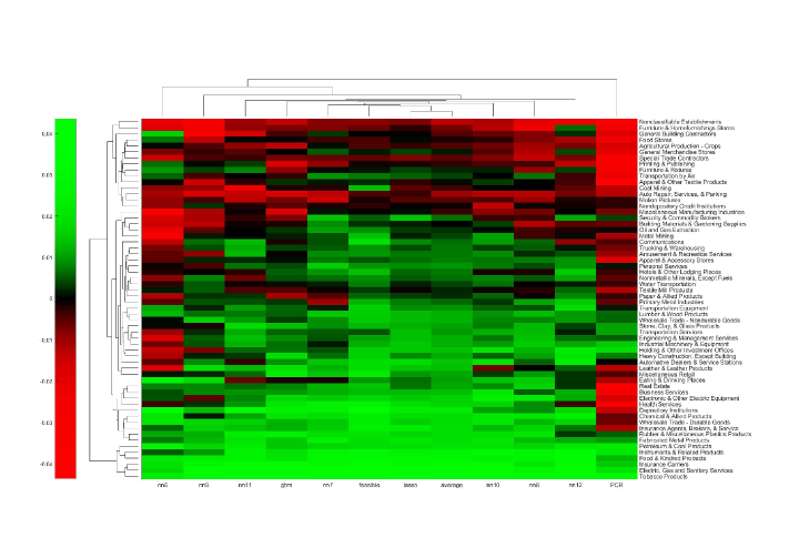
Figure 2: Heatmap of the prediction performance in terms of $R^{2}_{oos}$ for the equally-weighted sector returns from (1). Columns: Different machine learning models and meta-models. Rows: Different sectors. Two dendrogram trees showing clusters of models and sectors, respectively, in terms of their similarity in $R_{oos}^{2}$ values.

Figure 2 displays a comparison of machine learning techniques in terms of their $R^{2}_{oos}$ values across all 60 sectors using equally-weighted sector returns from (1). We compare a total of twelve models, including PCR, LASSO, gradient boosted regression trees (GBRT), neural networks architectures with six to twelve layers (NN6,$\ldots$, NN12), the meta-model with simple-averaging across models, and the feasible meta-strategy algorithms with the optimized learning rate. Figure 3 provides the same type of plot for capitalization-weighted sector returns. We observe that many models predict capitalization-weighted sector returns better than the equally-weighted sector returns. Multiple models provide positive $R^{2}_{oos}$ for each sector. Notably, it is impossible to select a single model for all sectors, and no sector has equal performance across all models. The ranking of models is sector-specific. The dendrograms on the sides of both figures show sectors with similar predictability across models and models with similar predictability across sectors. Thus, we develop a meta-algorithm that separately determines which models perform best in which sector and generates a joint prediction from all of them. Finally, Figures 2 and 3 show that the feasible ensemble algorithm outperform individual models in almost all sectors and for both sector return definitions.

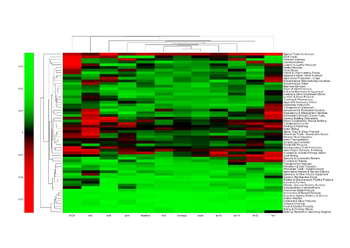
Figure 3: Similar to Figure 2 but for capitalization-weighted sector returns from (1).

4.2 Feature Importance

We assess the importance of features in predicting sector returns using the last 30-year rolling window and the ensemble weights from our pretrained model. Specifically, we compute the variable importance factors (VIFs) for each sector-level factor and all models within that sector using the method described in Greenwell and Boehmke, (2020). Next, we aggregate the VIFs for each sector by using the optimal weights from our pretrained ensemble algorithm. The resulting heatmaps and the vertical dendrograms in Figures 4 and 5 show the relative importance of different factors in predicting equally-weighted and capitalization-weighted sector returns, respectively. These results offer valuable insights into the attribution of predictability for different sector returns.

In our study, we aim to predict sector returns considering lead-lag relationships between features and returns as expressed in equations (2) and (3). The variable importance factors (VIFs) for most factors are typically small. Nevertheless, the remaining large VIF values are associated with factors that demonstrate a robust predictive relationship with sector returns. Figures 4 and 5 exhibit an intriguing pattern concerning sector clustering. We identify three primary sector clusters: the first includes sectors that can be predicted by nearly identical factors, the second contains sectors predictable by a diverse range of factors without a shared pattern, and the third comprises sectors that cannot be predicted by our factors. This clustering suggests that sectors can be grouped into three categories based on predictability: (i) predictable by common factors (top cluster in Figures 4 and 5), (ii) predictable by distinct factors (middle cluster in Figures 4 and 5), and (iii) not predictable by our factors (bottom cluster in Figures 4 and 5). For capitalization-weighted sector returns, the cluster with no positive VIFs is smaller, aligning with improved prediction outcomes for this kind of sector returns (Table 1). Our factors represent the first principal components in each sector, which are intended to predict significant variations within each sector. Consequently, large capitalization companies, which returns depend more on systematic risk, exhibit stronger predictability compared to small and mid-cap companies, which exhibit a lot of idiosyncratic risk. This leads to enhanced performance for all models in predicting capitalization-weighted sector returns, as illustrated in Figure 5.

The results in Figures 4 and 5 reveal that the predictability of factors varies depending on the sector, emphasizing the need to consider the sector-specific predictability of factors when constructing predictive models for sector returns. Despite that the PPCA method aggregets asset-specific factors into sector-level characteristics and leads to improved sector predictions, none of the factors predict all sectors, as shown by the heatmaps. In Figures 4 and 5 we highlight, the market beta and a few momentum factors, previously identified by Gu et al., (2020) as important predictors across individual stocks and models. In case of sector returns, the same factors exhibit varying degrees of predictability across sectors. This highlights the importance of identifying the most effective factors for each sector and incorporating them into the prediction model based on to which sector a given stock belongs.

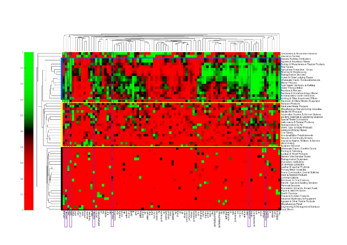
Figure 4: Heatmap of the variables importance factors (VIF) from the feasible ensemble method for the equally-weighted sector returns from (1) for the last rolling window January 1992 - December 2021 of data (VIF values are computed for each model and averaged using the weights from the feasible ensemble algorithm). Columns: Different features (see Appendix for a full list of our characteristics). The highlighted individual factors are market beta and various momentum indicators. Rows: Different sectors. Two dendrogram trees show clusters of features and sectors, respectively, in terms of their similarity in VIF values. Highlighted are three clusters of sectors: [top] predictable with common factors; [middle] predictable with a diversified set of factors; and [bottom] sectors that are difficult to predict using our factors.

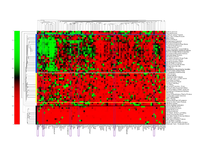
Figure 5: Similar to Figure 4 but for the capitalization-weighted sector returns from (1).

4.3 Sector Rotation Strategy

To evaluate the effectiveness of our ensemble algorithm, we construct a sector rotation strategy that ranks the sectors into five portfolios based on predicted returns from our feasible ensemble. Specifically, we sort the sectors in ascending order and allocate them into five quantile portfolios (“Bottom 5”, “41-55”, “21-40”, “6-20”, and “Top 5”). Each portfolio holds stocks from a given sector with the same weights as defined in (1). We report the performance results for both equally-weighted and capitalization-weighted sector returns. In addition, we use two benchmarks: the cumulative returns of an equally-weighted portfolio (“$1/N$”) and the S&P 500 index. Table 2 presents the annualized returns, volatilities, Sharpe ratios, maximum drawdowns, and Sortino ratios of the quantile portfolios and benchmarks over the entire out-of-sample period (Panel I A-B) and the recent two-year Covid-19 period (Panel II A-B). We examine the Covid-19 period separately due to significant economic and market changes during the pandemic. In particular, the S&P 500 index sharply dropped by $34\%$ in February-March 2020, followed by a recovery reaching $142\%$ of the pre-crisis peak. However, the recovery was uneven across sectors, with some recovering quickly, especially those related to healthcare, information technology, and consumer staples, while others, such as energy, industrials, utilities, real estate, and financials, lagged behind for an extended period. Our feasible ensemble model effectively captured these sector transitions in performance, generating large profits during this turbulent period. We also report the transaction cost analysis for the “Top 5” portfolio, where we present the same performance statistics for the net returns with 5, 10, and 15 basis points of linear transaction costs per percentage point of the turnover.

The performance of the quantile portfolios shows a clear improvement from the Bottom 5 to the Top 5, both in Panel I (A-B) for the whole out-of-sample period and in Panel II (A-B) for the Covid-19 period. The annualized returns increase steadily from $6.61\%$ to $14.15\%$ for the equally-weighted returns over the entire period, and from $19.15\%$ to $50.4\%$ during the Covid-19 period. The Top 5 portfolios also exhibit similar or slightly higher volatilities and maximum drawdowns compared to the benchmarks. However, the higher returns translate to the highest annualized Sharpe ratios and annualized Sortino ratios among all portfolios, both for the equally-weighted and capitalization-weighted sector returns. These results demonstrate the effectiveness of our ensemble algorithm in predicting sector returns and constructing a profitable sector rotation strategy, especially during periods of market turbulence such as the Covid-19 pandemic. We also analyze the impact of transaction costs on the performance of the Top 5 portfolio, and report the net returns for different levels of transaction costs.

The performance of the Top 5 sectors is impressive, with a Sortino ratio of 1.14 and 1.21 for the equally-weighted and capitalization-weighted strategies, respectively, over the entire out-of-sample period. In Panel II, we report the basic portfolio statistics for the constructed portfolios from January 2020 to December 2021. The Sharpe ratios of the Top 5 strategies are significantly higher than the benchmarks over the same period and the Top 5 strategies from the entire out-of-sample analysis. During this recent turbulent period, the strategy achieved Sortino ratios of $2.4$ and $2.1$ for equally-weighted and capitalization-weighted sector returns, respectively, outperforming the benchmarks (the $1/N$ strategy and the S&P 500 index). Hence, the strategy almost doubled its performance in recent years indicating that it is able to generate high returns by selecting better performing sectors even in turbulent periods.

Table 2: Portfolio statistics (“Annual Return”, “Annual Volatility”, “Annual Sharpe”, “Max. Drawdown”, and “Annual Sortino”) on portfolios. The predicted returns are calculated from meta-strategy. Each month we sort sectors in ascending order into quantile portfolios (“Bottom 5”, “41-55”, “21-40”, “6-20”, and “Top 5”) on the basis of predicted returns. The table also includes the benchmark portfolios market index (“S&P 500”) and (“1/N”), which is the average return across the 50 sectors. Panel I (A-B): 1987-2021. Panel II (A-B): Recent COVID-19 Period 2020-2021.

Statistics (1987-2021) S&P 500 1/N Bottom 5 41-55 21-40 6-20 Top 5 5BPs Net 10BPs 15BPs Panel I.A. Equally-Weighted Returns Annual Return 0.0889 0.1048 0.0661 0.0921 0.0983 0.1228 0.1415 0.1368 0.1322 0.1275 Annual Volatility 0.1504 0.1971 0.2304 0.2041 0.1951 0.1973 0.2153 0.2152 0.2151 0.2150 Annual Sharpe 0.5912 0.5317 0.2869 0.4511 0.5037 0.6225 0.6570 0.6357 0.6143 0.5931 Max. Drawdown 0.5256 0.6219 0.6639 0.6716 0.6204 0.5937 0.5233 0.5263 0.5292 0.5321 Annual Sortino 0.9487 0.9114 0.5903 0.8105 0.8640 1.0452 1.1465 1.1122 1.0782 1.0443 Panel I.B. Capital-Weighted Returns Annual Return 0.0889 0.1094 0.0950 0.0930 0.1117 0.1126 0.1385 0.1342 0.1300 0.1258 Annual Volatility 0.1504 0.1703 0.2064 0.1826 0.1686 0.1686 0.1883 0.1883 0.1883 0.1884 Annual Sharpe 0.5912 0.6422 0.4602 0.5093 0.6625 0.6676 0.7355 0.7129 0.6904 0.6679 Max. Drawdown 0.5256 0.5464 0.5995 0.5966 0.5617 0.4967 0.4825 0.4862 0.4899 0.4935 Annual Sortino 0.9487 1.0245 0.8132 0.8327 1.0657 1.0693 1.2190 1.1832 1.1477 1.1124 Statistics (2020-2021) S&P 500 1/N Bottom 5 41-55 21-40 6-20 Top 5 5BPs Net 10BPs 15BPs Panel II.A. Equally-Weighted Returns Annual Return 0.2162 0.2847 0.1915 0.3138 0.1925 0.3350 0.5040 0.4957 0.4875 0.4794 Annual Volatility 0.1954 0.3147 0.3623 0.3300 0.3336 0.2837 0.3324 0.3322 0.3320 0.3319 Annual Sharpe 1.1067 0.9049 0.5287 0.9507 0.5769 1.1807 1.5163 1.4922 1.4683 1.4444 Max. Drawdown 0.2000 0.3524 0.4569 0.3568 0.3896 0.2750 0.3173 0.3181 0.3190 0.3198 Annual Sortino 1.8400 1.5121 1.0014 1.6386 1.0437 2.0379 2.4006 2.3646 2.3287 2.2931 Panel II.B. Capital-Weighted Returns Annual Return 0.2162 0.2099 0.1955 0.1335 0.2396 0.2126 0.3073 0.3021 0.2970 0.2920 Annual Volatility 0.1954 0.2457 0.3273 0.2792 0.2361 0.2240 0.2410 0.2410 0.2410 0.2409 Annual Sharpe 1.1067 0.8545 0.5973 0.4782 1.0147 0.9495 1.2749 1.2538 1.2327 1.2117 Max. Drawdown 0.2000 0.2996 0.4178 0.3489 0.2835 0.2581 0.2300 0.2313 0.2327 0.2340 Annual Sortino 1.8400 1.3506 1.0135 0.8278 1.6604 1.4684 2.1066 2.0694 2.0325 1.9959

Although Table 2 provides aggregated results for the performance of our sector rotation strategy, it is important to examine how the performance of the proposed method evolves over time. This is especially crucial for advanced machine learning methods, which can rapidly lose their alpha signal due to market participants’ increasing access to alternative data and greater technological sophistication. To address this concern, we examine the monthly performance of our “Top 5” quantile of sectors as our sector rotation strategy. Figures 6 and 7 display the monthly performance of the strategy compared to the S&P 500 index, corresponding to equally- and capitalization-weighted sector returns from (1), respectively. The top panels of both figures present the cumulative returns, the middle panels show the monthly returns of the “Top 5”, and the bottom panels show the drawdowns of the strategy and the market. The results reveal that our sector rotation strategy has not been arbitraged out by other market participants, as the systematic outperformance of the strategy over the market grows over time. Particularly before and during the COVID-19 period, the out-of-sample performance of the strategy relative to the market is rapidly growing. This aligns with the intuition that we observed a rapid shift of investors towards specific sectors for example online technology and pharmaceutics during the pandemic, and our ensemble is able to capitalize on this shift and generate large profits.

In terms of drawdowns, both the equally-weighted and the capitalization-weighted “Top 5” strategies exhibit often smaller drawdowns than the market, and a much faster recovery from major market downturns such as the 2002 dot-com bubble and the 2008 global financial crisis. This highlights the potential of our strategy to provide downside protection and faster recovery from market shocks.

The long-term outperformance of the sector rotation strategy is consistent across both equally-weighted and capitalization-weighted sector returns, as demonstrated in Figures 6 and 7, as well as in Table 2. This implies that our strategy’s performance is not driven solely by less liquid and harder-to-trade small-cap stocks, which has important practical implications. By using capitalization-weighted portfolio weights within each sector, a ”Top 5” sectors strategy can hold larger positions in more liquid stocks, making it easier and less costly to trade, particularly for large institutional portfolios.

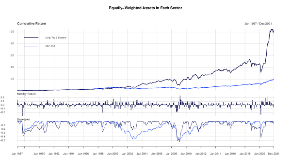
Figure 6: Performance summary plots for equally-weighted returns, as in (1), from January 1987 to December 2021. Top panel: a cumulative return plot over time for “Top 5” sectors long-only strategy, and S&P 500 index as a benchmark. Middle panel: a bar plot depicting monthly returns for the “Top 5” strategy. Bottom panel: an underwater plot shows drawdowns from cumulative returns attained over time for “Top 5” and the S&P 500.

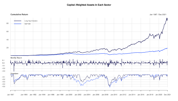
Figure 7: Performance summary plots for capital-weighted returns from (1). All the panels are the same as in Figure 6.

4.3.1 Robustness Checks

Table 3 provides insights into the performance of our feasible ensemble of machine learning models in predicting future returns of the sectors. The table reports the predicted returns, average excess return (“Excess return”), and alphas estimated from regression of excess portfolio returns on a constant and a set of systematic risk factors, proxied by three benchmark asset pricing models: (i) CAPM (Sharpe, , 1964), (ii) Fama-French three-factor model (Fama and French, , 1993), and (iii) Carhart four-factor model (Carhart, , 1997).

The ability of our ensemble model to accurately rank the future performance of the sectors is evident from the table, as the numbers in each row increase monotonically from the first quantile (“Bottom 5”) to the fifth quantile (“Top 5”). Additionally, the alphas for the “6-20” sectors-portfolio and the “Top 5” sectors-portfolio are all positive and significantly different from zero, mainly at $1\%$ level. This indicates that our sector rotation strategy captures some sector-aggregated characteristics yielding returns in addition to compensation for aggregated market-level risk factors.

Comparing across rows, we observe a monotonic decrease in the estimated alphas, suggesting that the excess market return, size, value, and momentum factors partially capture the returns generated by our sector rotation strategy. Nonetheless, the alphas remain positive and highly significant even after accounting for the effects of other factors, implying that the performance of our strategy cannot be explained solely by these well-known factors.

Finally, the last column of Table 3 shows the results for the market-neutral strategy, which invests long in the top five sectors and short in the bottom five sectors predicted by our feasible ensemble model. The alphas for this strategy are highly significant and very similar to the long-only “Top 5” strategy.

Table 3: Returns on portfolios selected by meta-strategy
This table reports average monthly returns on portfolios sorted by predicted returns over the sample period from Jan. 1987 to Dec. 2021. The predicted returns are calculated from the meta-strategy. Each month we sort sectors in ascending order into quantile portfolios (“Bottom 5”, “41-55”, “21-40”, “6-20”, and “Top 5”) on the basis of predicted returns. We also have a difference in monthly returns between the “Top 5” and “Bottom 5” portfolios (“Top-Bottom”). The top row (“Predicted return”) shows the average prediction of each portfolio. The remaining rows present excess returns (“Excess return”) and alphas from the Sharpe, (1964) model (“CAPM alpha”), from three-factor model (“3F alpha”) by Fama and French, (1993), and from Carhart four-factor model (“4F alpha”) by Carhart, (1997). Panel A presents results for equally- weighted strategy and Panel B for capital-weighted strategy. We report corrected $t$-values by Newey and West, (1987) in parentheses. *, **, and *** indicate significance at the 10%, 5%, and 1% levels, respectively.

Statistics	Bottom 5	41-55	21-40	6-20	Top 5	Top-Bottom
Panel A. Equally-Weighted Returns
Predicted return	0.0019	0.0067	0.0096	0.0125	0.0172	0.0177
Excess return	0.0076 **	0.0091 ***	0.0095 ***	0.0114 ***	0.0130 ***	0.0079 ***
	(2.0564)	(2.8666)	(3.0509)	(3.6262)	(3.9595)	(4.2205)
CAPM alpha	0.0014	0.0032	0.0036 *	0.0054 ***	0.0071 ***	0.0081 ***
	(0.5288)	(1.4026)	(1.8481)	(2.7691)	(3.0285)	(4.1263)
3F alpha	-0.0016	0.0004	0.0010	0.0028 ***	0.0047 ***	0.0088 ***
	(-0.9944)	(0.2670)	(0.9254)	(2.6207)	(2.9736)	(4.5865)
4F alpha	0.0010	0.0022	0.0026 ***	0.0039 ***	0.0053 ***	0.0068 ***
	(0.5971)	(1.6141)	(2.6925)	(3.4015)	(3.0470)	(4.0487)
Panel B. Capital-Weighted Returns
Predicted return	0.0008	0.0055	0.0084	0.0116	0.0178	0.0195
Excess return	0.0094 ***	0.0089 ***	0.0101 ***	0.0101 ***	0.0124 ***	0.0054 **
	(3.0388)	(3.6618)	(4.1568)	(4.5633)	(4.8145)	(2.4713)
CAPM alpha	0.0032	0.0027 *	0.0043 ***	0.0043 ***	0.0064 ***	0.0056 **
	(1.3212	(1.8506)	(3.2495)	(4.6785)	(3.7073)	(2.5342)
3F alpha	0.0003	0.0001	0.0019 **	0.0022 ***	0.0042 ***	0.0064 ***
	(0.1955)	(0.1330)	(2.3733)	(2.7900)	(2.9251)	(3.3200)
4F alpha	0.0020	0.0010	0.0023 ***	0.0023 ***	0.0035 **	0.0039 **
	(1.3503)	(1.0504)	(2.6683)	(3.0013)	(2.2045)	(2.0953)

Table 4 provides further evidence on the predictive power of our sector rotation strategy. We split the sample period into different subsamples based on specific economic conditions, such as the financial crisis of 2007-2008. We distinguish recession versus no-recession subsamples as indicated by the National Bureau of Economic Research Business Cycle Dating Committee. Above-average economic activity and below-average economic activity subsamples using an indicator based on whether the 3-month moving average of the Chicago Fed National Activity Index is negative or nonnegative, and the up-market and down-market subsamples using an indicator based on whether the S&P 500 index experienced a return in the month preceding portfolio formation that is negative or nonnegative.

For each subsample, we evaluate the performance of the “Bottom 5”, the “Top-5”, and the “Top-Bottom” strategies. Our results show that the “Top-5” strategy generates positive and significant excess returns in most subsamples, except for the recession subsample, which has a very small number of observations. The excess returns of the “Top 5” strategy is always much higher than the returns of the “Bottom 5”. Moreover, the market-neutral “Top-Bottom” portfolio exhibits a statistically significant positive effect in terms of excess returns across all subsamples. These findings suggest that the alphas generated by our sector rotation strategy are not driven by a specific period or market condition and are robust to different economic environments.

Table 4: Subsample analysis
This table reports average monthly returns on portfolios sorted by predicted returns after splitting our 1987-2021 sample period in a variety of ways. The predicted returns are calculated from the meta-strategy. The sample is split into two periods (i.e., 1987-2007 and 2008-2021). The recession and no-recession subsamples are indicated by the National Bureau of Economic Research Business Cycle Dating Committee. Above-average economic activity and below-average economic activity subsamples using an indicator based on whether the 3-month moving average of the Chicago Fed National Activity Index is negative or nonnegative, and the up-market and down-market subsamples using an indicator based on whether the Standard & Poor’s (S &P) 500 index experienced a return in the month preceding portfolio formation that is negative or nonnegative. Panel A presents results for equally- weighted strategy and Panel B for capital-weighted strategy. We report corrected $t$-values by Newey and West, (1987) in parentheses. *, **, and *** indicate significance at the 10%, 5%, and 1% levels, respectively.

Subsample	No. of Obs.	Bottom 5	Top 5	Top-Bottom
Panel A. Equally-Weighted Returns
1987-2007	252	0.0086 ***	0.0133 ***	0.0084 ***
		(2.8664)	(4.1927)	(4.2546)
2008-2021	168	0.0060	0.0126 **	0.0071 **
		(0.8291)	(2.0088)	(2.2727)
recession	36	-0.0068	0.0060	0.0150 *
		(-0.3171)	(0.2897)	(1.8076)
no recession	384	0.0089 ***	0.0137 ***	0.0072 ***
		(2.8484)	(4.6893)	(3.7405)
CFNAI$<$0	198	0.0025	0.0115 **	0.0113 ***
		(0.4307)	(2.2204)	(6.1180)
CFNAI$\geq$0	222	0.0121 ***	0.0144 ***	0.0049 **
		(3.0984)	(3.6389)	(2.0741)
SP&500 return$<$0	150	0.0069	0.0131 ***	0.0087 ***
		(1.2971)	(3.0085)	(3.1216)
SP&500 return$\geq$0	270	0.0080 *	0.0130 ***	0.0074 ***
		(1.8361)	(3.1969)	(3.7308)
Panel B. Capital-Weighted Returns
1987-2007	252	0.0094 ***	0.0132 ***	0.0076 ***
		(3.2472)	(4.1908)	(2.6182)
2008-2021	168	0.0095	0.0111 **	0.0021
		(1.6025)	(2.5748)	(0.6453)
recession	36	-0.0032	0.0004	0.0059
		(-0.1654)	(0.0270)	(1.5529)
no recession	384	0.0106 ***	0.0135 ***	0.0053 **
		(4.1160)	(6.5383)	(2.5426)
CFNAI$<$0	198	0.0056	0.0125 ***	0.0092 ***
		(1.1243)	(2.8136)	(3.4134)
CFNAI$\geq$0	222	0.0128 ***	0.0122 ***	0.0020
		(3.8777)	(4.8199)	(0.7274)
SP&500 return$<$0	150	0.0075	0.0128 ***	0.0077 **
		(1.5914)	(2.8302)	(2.5212)
SP&500 return$\geq$0	270	0.0105 ***	0.0122 ***	0.0041
		(2.9669)	(6.2262)	(1.6385)

5 Conclusion

We present a novel online ensemble algorithm that fuses various models according to their historical out-of-sample performance. This algorithm employs the gradient-free Multiplicative Weights Update Method and introduces a new cost function for updating ensemble weights.

The proposed cost function balances exploration and exploitation trade-offs, enabling us to learn an ensemble that achieves the highest out-of-sample $R^{2}$. Utilizing regret bounds derived from online optimization theory, we demonstrate that the risk premium of the resulting ensemble model will closely approximate the risk premium of an infeasible ensemble that presumes knowledge of the best ensemble weights from the outset.

Monti et al., (2018) and Capó et al., (2022) propose gradient-based online algorithms for adaptive regularization in LASSO regression. Our algorithm can also be applied to hyperparameter tuning. However, similarly to standard cross-validation, it is gradient free. Moreover, instead of out-of-sample $R^{2}$, the algorithm can minimize, as in Monti et al., , 2018, the predicted mean squared error. In that case all the results presented in this paper would hold for any finite $\tau$ because the predicted mean-squared error does not require a volatility estimation.

Empirically, our paper demonstrates that information from individual stocks aggregated to sector level characteristics, lead to more accurate sector predictions, and that our ensemble of machine learning models predicts sector returns even better than the individual models.

Neely et al., (2014) demonstrate that technical indicators and macroeconomic variables offer complementary information regarding the dynamics of the business cycles, and lead to profitable sector rotation strategies. An intriguing avenue for future research is to investigate whether macroeconomic variables can complement our sector-level factors and be jointly employed in machine learning models to enhance the profitability of sector rotation strategies.

Appendix

A: Proofs

We start with the proof of Lemma 3.1.

Proof.

The $\tau$ periods $R^{2}_{oos}$ can be written as

$$R_{oos}^{2}(\tau) =1-\frac{\sum_{t=1}^{\tau}(r_{t}-\tilde{r}_{t})^{2}}{\sum_{t=1}^{\tau}r_{t}^{2}}=1-\frac{\frac{1}{\tau}\sum_{t=1}^{\tau}(r_{t}-\tilde{r}_{t})^{2}}{\frac{1}{\tau}\sum_{t=1}^{\tau}r_{t}^{2}}=\frac{1}{\tau}\sum_{t=1}^{\tau}\left(1-\frac{(r_{t}-\tilde{r}_{t})^{2}}{\frac{1}{\tau}\sum_{t=1}^{\tau}r_{t}^{2}}\right)$$

$$=\frac{1}{\tau}\sum_{t=1}^{\tau}\left(1-\frac{(r_{t}-\widehat{\mathbf{r}}_{t}^{\top}\mathbf{p}^{(t)})^{2}}{\widehat{\sigma}_{t}^{2}}\frac{\widehat{\sigma}_{t}^{2}}{\frac{1}{\tau}\sum_{t=1}^{\tau}r_{t}^{2}}\right)$$

$$=\frac{1}{\tau}\sum_{t=1}^{\tau}\left(1-\frac{r_{t}^{2}-2r_{t}\widehat{\mathbf{r}}_{t}^{\top}\mathbf{p}^{(t)}+(\widehat{\mathbf{r}}_{t}^{\top}\mathbf{p}^{(t)})^{2}}{\widehat{\sigma}_{t}^{2}}\frac{\widehat{\sigma}_{t}^{2}}{\frac{1}{\tau}\sum_{t=1}^{\tau}r_{t}^{2}}\right)$$

$$=\frac{1}{\tau}\sum_{t=1}^{\tau}\left(1-\left[\frac{r_{t}^{2}-2r_{t}\widehat{\mathbf{r}}_{t}^{\top}\mathbf{p}^{(t)}}{\widehat{\sigma}_{t}^{2}}+\frac{(\widehat{\mathbf{r}}_{t}^{\top}\mathbf{p}^{(t)})^{2}}{\widehat{\sigma}_{t}^{2}}\right]\frac{\widehat{\sigma}_{t}^{2}}{\frac{1}{\tau}\sum_{t=1}^{\tau}r_{t}^{2}}\right),$$ (9)

where

• $r_{t}$ sector return

• $\widehat{\mathbf{r}}_{t}=\left[\widehat{{r}}_{t,1},\ldots,\widehat{{r}}_{t,L}\right]^{\top}$ vector of the predicted returns (for a given sector) from $L$ different prediction models at rolling window $t$

• $\mathbf{p}^{(t)}=\left[{p}_{1}^{(t)},\ldots,{p}_{L}^{(t)}\right]^{\top}$, and $p_{l}^{(t)}$ the weight of each model $l=1,\ldots,L$ at time $t$

• $\left\{\widetilde{r}_{t}\right\}_{t=1,\ldots,\tau}=\widehat{\mathbf{r}}_{t}^{\top}\mathbf{p}^{(t)}$ the weighted combination of predictions of all the experts at time $t$

• $\widehat{\sigma}_{t}^{2}=\frac{1}{\tau}\sum_{s^{(t)}=1}^{\tau}r_{s^{(t)}}^{2}$ is the bootstrap estimate of the second moment of the sector returns based on the past $t$ observations

• $\mathbbm{1}_{L}=[1,\ldots,1]^{\top}\in\mathbb{R}^{L}$, and by the properties of the multiplicative weights update method $\mathbbm{1}_{L}^{\top}\mathbf{p}^{(t)}=1$.

Note that in the last equation in (9) we can replace $(\widehat{\mathbf{r}}_{t}^{\top}\mathbf{p}^{(t)})^{2}$ with

$$(\widehat{\mathbf{r}}_{t}^{\top}\mathbf{p}^{(t)})^{2}=\left[\widehat{r}_{t,1}^{2},\ldots,\widehat{r}_{t,L}^{2}\right]^{\top}\left[(p_{1}^{(t)})^{2},\ldots,(p_{L}^{(t)})^{2}\right]+R_{t},$$ (10)

where

$$R_{t}=\sum_{i=1}^{L}\sum_{j=1\\ j\neq i}^{L}\widehat{r}_{t,i}p_{i}^{(t)}\widehat{r}_{t,j}p_{j}^{(t)}.$$

The key term in (9) is $\frac{(r_{t}-\widehat{\mathbf{r}}_{t}^{\top}\mathbf{p}^{(t)})^{2}}{\widehat{\sigma}_{t}^{2}}$, which is not linear in the ensemble weights $\mathbf{p}^{(t)}$. Therefore, we consider a similar term,

$$\left[\frac{(r_{t}\mathbbm{1}_{L}-\widehat{\mathbf{r}}_{t})^{2}}{\widehat{\sigma}_{t}^{2}}\right]^{\top}\mathbf{p}^{(t)} =\frac{r_{t}^{2}\mathbbm{1}_{L}^{\top}\mathbf{p}^{(t)}-2r_{t}\widehat{\mathbf{r}}_{t}^{\top}\mathbf{p}^{(t)}+\widehat{\mathbf{r}}_{t}^{2\top}\mathbf{p}^{(t)}}{\widehat{\sigma}_{t}^{2}}$$

$$\overset{\mathbbm{1}_{L}^{\top}\mathbf{p}^{(t)}=1}{=}\frac{r_{t}^{2}-2r_{t}\widehat{\mathbf{r}}_{t}^{\top}\mathbf{p}^{(t)}}{\widehat{\sigma}_{t}^{2}}+\frac{\widehat{\mathbf{r}}_{t}^{2\top}\mathbf{p}^{(t)}}{\widehat{\sigma}_{t}^{2}}$$

where $\widehat{\mathbf{r}}_{t}^{2\top}=\left[\widehat{r}_{t,1}^{2},\ldots,\widehat{r}_{t,L}^{2}\right]^{\top}$ and we relate the two quantities via the following function and its Taylor series expansion

$$\varphi_{t}(\mathbf{x}_{t},y_{t})=(\alpha_{t}+\mathbf{b}_{t}^{\top}\mathbf{x}_{t}+\frac{R_{t}}{\widehat{\sigma}_{t}^{2}})y_{t}$$

where

$$\alpha_{t}=\left(\frac{r_{t}^{2}\mathbbm{1}_{L}-2r_{t}\widehat{\mathbf{r}}_{t}}{\widehat{\sigma}_{t}^{2}}\right)^{\top}\mathbf{p}^{(t)}\in\mathbb{R}\ \mbox{and}\ \mathbf{b}_{t}=\frac{\left[\widehat{r}_{t,1}^{2}p_{1}^{(t)},\ldots,\widehat{r}_{t,L}^{2}p_{L}^{(t)}\right]^{\top}}{\widehat{\sigma}_{t}^{2}}\in\mathbb{R}^{\mathrm{L}}$$

Then we have

$$\varphi_{t}(\mathbf{x}_{t},y_{t})=\begin{cases}\frac{(r_{t}-\tilde{r}_{t})^{2}}{\frac{1}{\tau}\sum_{t=1}^{\tau}r_{t}^{2}}&\mbox{for}\ \mathbf{x_{t}}=\mathbf{p}^{(t)}\ \mbox{and}\ y_{t}=\frac{\widehat{\sigma}_{t}^{2}}{\frac{1}{\tau}\sum_{t=1}^{\tau}r_{t}^{2}}\\ \left[\frac{(r_{t}\mathbbm{1}_{L}-\widehat{\mathbf{r}}_{t})^{2}}{\widehat{\sigma}_{t}^{2}}\right]^{\top}\mathbf{p}^{(t)}+\frac{R_{t}}{\widehat{\sigma}_{t}^{2}}&\mbox{for}\ \mathbf{x_{0}}=\mathbbm{1}_{L}\ \mbox{and}\ y_{0}=1\end{cases}$$

and the corresponding partial derivatives are

$$\frac{\partial\varphi_{t}}{\partial\mathbf{x}} =y_{t}\mathbf{b}_{t}^{\top},\quad\frac{\partial\varphi_{t}}{\partial y}=\alpha_{t}+\mathbf{b}_{t}^{\top}\mathbf{x}+\frac{R_{t}}{\widehat{\sigma}_{t}^{2}},$$

$$\frac{\partial\varphi_{t}}{\partial\mathbf{x}\partial y} =\mathbf{b}_{t}^{\top},\quad\frac{\partial\varphi_{t}^{k+l}}{\partial x_{i}^{k}\partial x_{j}^{l}}=0,\quad\forall\,k\geq 1,\ \forall\,l\geq 1,$$

$$\frac{\partial\varphi_{t}^{k+l}}{\partial x_{i}^{k}\partial y^{l}}=0,\quad\forall\,k,l:\max(k,l)>1,\ \forall\,i=1,\ldots,L.$$ (11)

So, for the function $\varphi_{t}(\mathbf{x}_{t},y_{t})$, Taylor’s expansion at the point $(\mathbf{x_{0}},y_{0})$ is given by

$$\varphi_{t}(\mathbf{x}_{t},y_{t}) =\varphi_{t}(\mathbf{x}_{0},y_{0})+\frac{\partial\varphi_{t}}{\partial\mathbf{x}}\mid_{\mathbf{x}=\mathbf{x}_{0},y=y_{0}}(\mathbf{x_{t}}-\mathbf{x_{0}})$$

$$+\frac{\partial\varphi_{t}}{\partial y}\mid_{\mathbf{x}=\mathbf{x}_{0},y=y_{0}}(y_{t}-y_{0})+\frac{\partial\varphi_{t}^{2}}{\partial\mathbf{x}\partial y}\mid_{\mathbf{x}=\mathbf{x}_{0},y=y_{0}}(\mathbf{x_{t}}-\mathbf{x_{0}})(y_{t}-y_{0}).$$ (12)

Then we have

$$\frac{(r_{t}-\tilde{r}_{t})^{2}}{\frac{1}{\tau}\sum_{t=1}^{\tau}r_{t}^{2}} =\left[\frac{(r_{t}\mathbbm{1}_{L}-\widehat{\mathbf{r}}_{t})^{2}}{\widehat{\sigma}_{t}^{2}}\right]^{\top}\mathbf{p}^{(t)}+\frac{R_{t}}{\widehat{\sigma}_{t}^{2}}+\mathbf{b}_{t}^{\top}(\mathbf{x_{t}}-\mathbf{x_{0}})$$

$$+(\alpha_{t}+\mathbf{b}_{t}^{\top}\mathbbm{1}_{L}+\frac{R_{t}}{\widehat{\sigma}_{t}^{2}})(y_{t}-y_{0})+\mathbf{b}_{t}^{\top}(\mathbf{x_{t}}-\mathbf{x_{0}})(y_{t}-y_{0}),$$ (13)

So

$$1-\frac{(r_{t}-\tilde{r}_{t})^{2}}{\frac{1}{\tau}\sum_{t=1}^{\tau}r_{t}^{2}} =1-\left[\frac{(r_{t}\mathbbm{1}_{L}-\widehat{\mathbf{r}}_{t})^{2}}{\widehat{\sigma}_{t}^{2}}\right]\mathbf{p}^{(t)}-\frac{R_{t}}{\widehat{\sigma}_{t}^{2}}-\mathbf{b}_{t}^{\top}(\mathbf{x_{t}}-\mathbf{x_{0}})$$

$$-(\alpha_{t}+\mathbf{b}_{t}^{\top}\mathbbm{1}_{L}+\frac{R_{t}}{\widehat{\sigma}_{t}^{2}})(y_{t}-y_{0})-\mathbf{b}_{t}^{\top}(\mathbf{x_{t}}-\mathbf{x_{0}})(y_{t}-y_{0}),$$

and

$$R_{oos}^{2}(\tau) =\frac{1}{\tau}\sum_{t=1}^{\tau}\left(1-\frac{(r_{t}-\tilde{r}_{t})^{2}}{\frac{1}{\tau}\sum_{t=1}^{\tau}r_{t}^{2}}\right)=\frac{1}{\tau}\sum_{t=1}^{\tau}\left(\mathbbm{1}_{L}^{\top}\mathbf{p}^{(t)}-\left[\frac{(r_{t}\mathbbm{1}_{L}-\widehat{\mathbf{r}}_{t})^{2}}{\widehat{\sigma}_{t}^{2}}\right]^{\top}\mathbf{p}^{(t)}-\frac{R_{t}}{\widehat{\sigma}_{t}^{2}}-\mathbf{b}_{t}^{\top}(\mathbf{x_{t}}-\mathbf{x_{0}})\right)$$

$$-\frac{1}{\tau}\sum_{t=1}^{\tau}\left((\alpha_{t}+\mathbf{b}_{t}^{\top}\mathbbm{1}+\frac{R_{t}}{\widehat{\sigma}_{t}^{2}})(y_{t}-y_{0})+\mathbf{b}_{t}^{\top}(\mathbf{x_{t}}-\mathbf{x_{0}})(y_{t}-y_{0})\right).$$

Note that

$$\mathbf{b}_{t}^{\top}(\mathbf{x_{t}}-\mathbf{x_{0}})=\frac{\left[\widehat{r}_{t,1}^{2}p_{1}^{(t)},\ldots,\widehat{r}_{t,L}^{2}p_{L}^{(t)}\right]^{\top}}{\widehat{\sigma}_{t}^{2}}(\mathbf{p}^{(t)}-\mathbbm{1}_{L})=\frac{\left[(\widehat{r}_{t,1}^{2}p_{1}^{(t)}-\widehat{r}_{t,1}^{2}),\ldots,(\widehat{r}_{t,L}^{2}p_{L}^{(t)}-\widehat{r}_{t,L}^{2})\right]^{\top}}{\widehat{\sigma}_{t}^{2}}\mathbf{p}^{(t)}.$$

Hence,

$$R_{oos}^{2}(\tau) =\frac{1}{\tau}\sum_{t=1}^{\tau}\left(\mathbbm{1}_{L}^{\top}\mathbf{p}^{(t)}-\left[\frac{(r_{t}\mathbbm{1}_{L}-\widehat{\mathbf{r}}_{t})^{2}}{\widehat{\sigma}_{t}^{2}}\right]^{\top}\mathbf{p}^{(t)}-\frac{R_{t}}{\widehat{\sigma}_{t}^{2}}-\frac{\left[(\widehat{r}_{t,1}^{2}p_{1}^{(t)}-\widehat{r}_{t,1}^{2}),\ldots,(\widehat{r}_{t,L}^{2}p_{L}^{(t)}-\widehat{r}_{t,L}^{2})\right]^{\top}}{\widehat{\sigma}_{t}^{2}}\text{$\mathbf{p}^{(t)}$}\right)$$

$$-\frac{1}{\tau}\sum_{t=1}^{\tau}\left((\alpha_{t}+\mathbf{b}_{t}^{\top}\mathbbm{1}_{L}+\frac{R_{t}}{\widehat{\sigma}_{t}^{2}})(y_{t}-y_{0})+\mathbf{b}_{t}^{\top}(\mathbf{x_{t}}-\mathbf{x_{0}})(y_{t}-y_{0})\right)$$

$$=\frac{1}{\tau}\sum_{t=1}^{\tau}\left(\mathbbm{1}_{L}-\frac{(r_{t}\mathbbm{1}-\widehat{\mathbf{r}}_{t})^{2}}{\widehat{\sigma}_{t}^{2}}-\frac{(\widetilde{R}_{t}\mathbbm{1})}{\widehat{\sigma}_{t}^{2}}\right)^{\top}\mathbf{p}^{(t)}-\frac{1}{\tau}\sum_{t=1}^{\tau}\left(\frac{(r_{t}\mathbbm{1}_{L}-\widehat{\mathbf{r}}_{t})^{2}+\widetilde{R}_{t}\mathbbm{1}}{\widehat{\sigma}_{t}^{2}}\right)^{\top}\mathbf{p}^{(t)}(y_{t}-y_{0}),$$

where $\widetilde{R}_{t}=\left[\xi_{i,j,t}\right]_{i=1,\ldots,L}^{j=1,\ldots,L}$ is an $L\times L$ matrix with

$$\xi_{i,j,t}=\begin{cases}\widehat{r}_{t,i}\widehat{r}_{t,j}p_{j}^{(t)}&\mbox{if }i\neq j\\ -\widehat{r}^{2}_{t,i}(1-p_{i}^{(t)})&\mbox{otherwise.}\end{cases}$$

If we define the gain function as

$$\mathbf{m}^{(t)}(\mathbf{p}^{(t)})=\left[\mathbbm{1}_{L}\ -\frac{(r_{t}\mathbbm{1}_{L}-\widehat{\mathbf{r}}_{t})^{2}}{\widehat{\sigma}_{t}^{2}}-\frac{\widetilde{R}_{t}\mathbbm{1}}{\widehat{\sigma}_{t}^{2}}\right],$$

then

$$R_{oos}^{2}(\tau)-\frac{1}{\tau}\sum_{t=1}^{\tau}\mathbf{m}^{(t)}(\mathbf{p}^{(t)})^{\top}\mathbf{p}^{(t)} =-\frac{1}{\tau}\sum_{t=1}^{\tau}\left(\frac{(r_{t}\mathbbm{1}_{L}-\widehat{\mathbf{r}}_{t})^{2}+\widetilde{R}_{t}\mathbbm{1}_{L}}{\widehat{\sigma}_{t}^{2}}\right)^{\top}\mathbf{p}^{(t)}(y_{t}-y_{0})$$

$$=-\frac{1}{\tau}\sum_{t=1}^{\tau}(1-\mathbf{m}^{(t)}(\mathbf{p}^{(t)})^{\top}\mathbf{p}^{(t)})(y_{t}-y_{0}),$$

and

$$\lim_{\tau\rightarrow\infty} \left|-\frac{1}{\tau}\sum_{t=1}^{\tau}(1-\mathbf{m}^{(t)}(\mathbf{p}^{(t)})^{\top}\mathbf{p}^{(t)})(y_{t}-y_{0})\right|\leq\lim_{\tau\rightarrow\infty}\frac{1}{\tau}\sum_{t=1}^{\tau}\left|(1-\mathbf{m}^{(t)}(\mathbf{p}^{(t)})^{\top}\mathbf{p}^{(t)})(y_{t}-y_{0})\right|$$

$$\leq\lim_{\tau\rightarrow\infty}\frac{1}{\tau}\sum_{t=1}^{\tau}\left|\ 1-\mathbf{m}^{(t)}(\mathbf{p}^{(t)})^{\top}\mathbf{p}^{(t)}\right|\left|y_{t}-y_{0}\right|\leq C\lim_{\tau\rightarrow\infty}\frac{1}{\tau}\sum_{t=1}^{\tau}\left|y_{t}-y_{0}\right|=0,$$

where in the last inequality we use that for some $C>0$, for all $t$,

$$\left|1-\mathbf{m}^{(t)}(\mathbf{p}^{(t)})^{\top}\mathbf{p}^{(t)}\right|\leq C,$$

and the limit holds because $\widehat{\sigma}_{\tau}^{2}$ and $\frac{1}{\tau}\sum_{t=1}^{\tau}r_{t}^{2}$ both are consistent and bounded estimators of the second moment of $r_{t}$. So we have

$$\left|R_{oos}^{2}(\tau)-\frac{1}{\tau}\sum_{t=1}^{\tau}\mathbf{m}^{(t)}(\mathbf{p}^{(t)})\top\mathbf{p}^{(t)}\right|\overset{a.s.}{\rightarrow}0\quad\mbox{as}\quad\tau\rightarrow\infty.$$

∎

Next we prove Theorem 3.1.

Proof.

Because of the linearity of the gain function $\mathbf{m}^{(t)}(\mathbf{p}^{(t)})$, we can write it as

$$\mathbf{m}^{(t)}(\mathbf{p}^{(t)})=\mathbf{m}^{(t)}(\mathbf{p}^{*})+\mathbf{H}_{t}(\mathbf{p}^{(t)}-\mathbf{p}^{*}),$$

where $\mathbf{H}_{t}=\widehat{\mathbf{r}}_{t}\widehat{\mathbf{r}}_{t}^{\top}$.

Hence, Corollary 2.6 in Arora et al., (2012), implies that

$$\lim_{\tau\rightarrow\infty}R_{oos}^{2}(\tau)\geq\lim_{\tau\rightarrow\infty}\left\{R_{oos}^{2*}(\tau)+\frac{1}{\tau}\sum_{t=1}^{\tau}(\mathbf{p}^{(t)}-\mathbf{p}^{*})^{\top}\widehat{\mathbf{r}}_{t}\widehat{\mathbf{r}}^{\top}_{t}\mathbf{p}^{*}-\eta\frac{1}{\tau}\sum_{t=1}^{\tau}\left|\mathbf{m}^{(t)}(\mathbf{p}^{(t)})\right|^{\top}\mathbf{p}^{*}-\frac{\log L}{\tau\eta}\right\}.$$

∎

Next, we prove the result in Corollary 3.1.

Proof.

Using Cauchy-Schwarz inequality on the upper bound in Theorem3.1 and since $\left\|\mathbf{p}^{*}\right\|_{2}^{2}\leq 1$, we have that

$$\frac{1}{\tau}\sum_{t=1}^{\tau}\left|\mathbf{m}^{(t)}(\mathbf{p}^{(t)})\right|^{\top}\mathbf{p}^{*} \leq\left\|\frac{1}{\tau}\sum_{t=1}^{\tau}\left|\mathbf{m}^{(t)}(\mathbf{p}^{(t)})\right|\right\|_{2}$$ (14)

∎

Next, we prove the result in Corollary 3.2

Proof.

From Corollary 2.2 in Arora et al., (2012) we get that

$$\lim_{\tau\rightarrow\infty}R_{oos}^{2}(\tau)\geq\lim_{\tau\rightarrow\infty}\left\{R_{oos}^{2*}(\tau)-\left(\eta\frac{1}{\tau}\sum_{t=1}^{\tau}\left|\mathbf{m}^{(t)}(\mathbf{p}^{(t)})\right|^{\top}\mathbf{p}^{*}+\frac{\log L}{\eta}\right)\right\}.$$ (15)

Since $\mathbf{p}^{*}\geq 0$, using Young’s inequality, for any $\lambda>0$, we get

$$\frac{1}{\tau}\sum_{t=1}^{\tau}\left|\mathbf{m}^{(t)}(\mathbf{p}^{(t)})\right|^{\top}\mathbf{p}^{*} \leq\frac{\lambda}{2}\left\|\mathbf{p}^{*}\right\|_{2}^{2}+\frac{1}{\lambda}\left\|\frac{1}{\tau}\sum_{t=1}^{\tau}\left|\mathbf{m}^{(t)}(\mathbf{p}^{(t)})\right|\right\|_{2}^{2}\leq\frac{\lambda}{2}+\frac{1}{2\lambda}\left\|\frac{1}{\tau}\sum_{t=1}^{\tau}\left|\mathbf{m}^{(t)}(\mathbf{p}^{(t)})\right|\right\|_{2}^{2},$$ (16)

where the second inequality holds because $\left\|\mathbf{p}^{*}\right\|_{2}^{2}\leq 1$, Since the last inequality holds for any $\lambda>0$ we can consider

$$f(\lambda)=\frac{\lambda}{2}+\frac{1}{2\lambda}\left\|\frac{1}{\tau}\sum_{t=1}^{\tau}\left|\mathbf{m}^{(t)}(\mathbf{p}^{(t)})\right|\right\|_{2}^{2}.$$

The minimum of that function is at $\lambda^{*}=\left\|\frac{1}{\tau}\sum_{t=1}^{\tau}\left|\mathbf{m}^{(t)}(\mathbf{p}^{(t)})\right|\right\|_{2}$. Hence, the tightest bound we can get in (16) is

$$\frac{1}{\tau}\sum_{t=1}^{\tau}\left|\mathbf{m}^{(t)}(\mathbf{p}^{(t)})\right|^{\top}\mathbf{p}^{*} \leq\left\|\frac{1}{\tau}\sum_{t=1}^{\tau}\left|\mathbf{m}^{(t)}(\mathbf{p}^{(t)})\right|\right\|_{2}.$$ (17)

Hence, we can further modify the bound in (15) to

$$\lim_{\tau\rightarrow\infty}R_{oos}^{2}(\tau)\geq\lim_{\tau\rightarrow\infty}\left\{R_{oos}^{2*}(\tau)-\left(\eta\left\|\frac{1}{\tau}\sum_{t=1}^{\tau}\left|\mathbf{m}^{(t)}(\mathbf{p}^{(t)})\right|\right\|_{2}+\frac{\log L}{\eta}\right)\right\}.$$ (18)

Now, the minimum of function

$$g(\eta)=\left(\eta\left\|\frac{1}{\tau}\sum_{t=1}^{\tau}\left|\mathbf{m}^{(t)}(\mathbf{p}^{(t)})\right|\right\|_{2}+\frac{\log L}{\eta}\right),$$

with respect to $\eta>0$ is given by

$$\eta^{*}=\sqrt{\frac{\log L}{\left\|\frac{1}{\tau}\sum_{t=1}^{\tau}\left|\mathbf{m}^{(t)}(\mathbf{p}^{(t)})\right|\right\|_{2}}}.$$

When plugged into (18), it gives the result. ∎

Next, we need to derive the closed form solution for the optimal $\mathbf{p}^{*}$ and the bound for it given in Lemma 3.2

Proof.

The objective function in (6) is a quadratic and the equality constraints are linear. Hence, it is a convex problem that has a unique minimum. In order to determine it, we can write the Lagrangian $\mathcal{L}$ for simpler equivalent problem. Namely,

$$\mathcal{L}(\mathbf{p},\lambda)=\frac{1}{\tau}\sum_{t=1}^{\tau}(r_{t}-\widehat{\mathbf{r}}_{t}^{\top}\mathbf{p})^{2}-2\lambda(\mathbbm{1}_{L}^{\top}\mathbf{p}-1).$$

Setting the first derivatives of $\mathcal{L}$ to zero and using matrix notation gives a system of $L+1$ linear equations in $\widehat{\mathbf{p}}^{*}$ and $\lambda$:

$$\begin{bmatrix}\widehat{\mathbf{r}}^{\top}\widehat{\mathbf{r}}&\mathbbm{1}_{L}\\ \mathbbm{1}^{\top}_{L}&0\\ \end{bmatrix}\begin{bmatrix}\widehat{\mathbf{p}}^{*}\\ \lambda\end{bmatrix}=\begin{bmatrix}\widehat{\mathbf{r}}^{\top}\mathbf{r}\\ 1\end{bmatrix}$$

where $\widehat{\mathbf{r}}=\left[\widehat{\mathbf{r}}^{\top}_{1},\ldots,\widehat{\mathbf{r}}_{\tau}^{\top}\right]^{\top}$ is a $\tau\times L$ matrix of predicted returns, and $\mathbf{r}=[r_{1},\ldots,r_{\tau}]^{\top}$ is the $\tau\times 1$ vector of realized returns. Assuming invertibility of the $L\times L$ matrix $\widehat{\mathbf{r}}^{\top}\widehat{\mathbf{r}}$, we get

$$\widehat{\mathbf{p}}^{*}=\widehat{\mathbf{p}}_{\mbox{\tiny OLS\normalsize}}-(\widehat{\mathbf{r}}^{\top}\widehat{\mathbf{r}})^{-1}\mathbbm{1}_{L}\lambda,$$

where $\widehat{\mathbf{p}}_{\mbox{\tiny OLS\normalsize}}=(\widehat{\mathbf{r}}^{\top}\widehat{\mathbf{r}})^{-1}\widehat{\mathbf{r}}^{\top}\mathbf{r}$ is the solution to the corresponding unconstrained least problem. Then, from the second equation, we get

$$\mathbbm{1}_{L}^{\top}(\widehat{\mathbf{r}}^{\top}\widehat{\mathbf{r}})^{-1}\mathbbm{1}_{L}\lambda=\mathbbm{1}_{L}^{\top}\widehat{\mathbf{p}}_{\mbox{\tiny OLS\normalsize}}-1$$

which we can solve for $\lambda$. Combining

$$\widehat{\mathbf{p}}^{*}=\widehat{\mathbf{p}}_{\mbox{\tiny OLS\normalsize}}-(\widehat{\mathbf{r}}^{\top}\widehat{\mathbf{r}})^{-1}\mathbbm{1}_{L}\frac{\mathbbm{1}_{L}^{\top}\widehat{\mathbf{p}}_{\mbox{\tiny OLS\normalsize}}-1}{\mathbbm{1}_{L}^{\top}(\widehat{\mathbf{r}}^{\top}\widehat{\mathbf{r}})^{-1}\mathbbm{1}_{L}},$$

and it gives the closed form expression for the optimal $\widehat{\mathbf{p}}^{*}$.

The bound $\left\|\widehat{\mathbf{p}}^{*}\right\|_{2}\leq\delta_{\tau}$, follows from the closed form expression for the optimal $\widehat{\mathbf{p}}^{*}$, where $\left\|(\frac{1}{\tau}\sum_{t=1}^{\tau}\widehat{\mathbf{r}}_{t}\widehat{\mathbf{r}}_{t}^{\top})^{-1}\mathbf{y}\right\|_{2}\leq\left\|(\frac{1}{\tau}\sum_{t=1}^{\tau}\widehat{\mathbf{r}}_{t}\widehat{\mathbf{r}}_{t}^{\top})^{-1}\right\|_{2}\left\|\mathbf{y}\right\|_{2}$ for any $\mathbf{y}\in\mathbb{R}^{L}$, and $\lambda^{-1}_{min}=\left\|(\frac{1}{\tau}\sum_{t=1}^{\tau}\widehat{\mathbf{r}}_{t}\widehat{\mathbf{r}}_{t}^{\top})^{-1}\right\|_{2}$, where $\lambda_{min}$ is the smallest eigenvalue of the matrix $\frac{1}{\tau}\sum_{t=1}^{\tau}\widehat{\mathbf{r}}_{t}\widehat{\mathbf{r}}_{t}^{\top}$. But also, since all the weights are non-negative and sum up to $1$, $\left\|\widehat{\mathbf{p}}^{*}\right\|_{2}\leq 1$. Combining, we get $\left\|\widehat{\mathbf{p}}^{*}\right\|_{2}\leq\min(1,\delta_{\tau})$. ∎

B: Probabilistic Principal Component Analysis

Principal component analysis (PCA) is a well-established method for dimension reduction. As introduced by Pearson, (1901), and later developed by Hotelling, (1933), the PCA projects the original sample of data into a new space. Hotelling, (1936) described it as finding proximities that summarize information by maximizing the variance. For a centered data matrix $X\in\mathbb{R}^{k\times t}$ where $t$ is the number of the observations and $k$ is the number of feature measurements, the sample covariance matrix $S$ can be given as

$$S=\frac{1}{T}XX^{\top}.$$ (19)

Thus, the orthogonal matrix $W\in\mathbb{R}^{k\times q}$ (also referred to as transformation matrix) is composed of $q$ dominant eigenvectors that are related to the corresponding largest eigenvalues of $S$. The associated principal components (latent variables) or scores $F\in\mathbb{R}^{q\times t}$, become

$$F=W^{\top}X.$$ (20)

It is doable to calculate matrix $W$ only on complete matrices via singular value decomposition (SVD) or the covariance matrix $S$. If we have missing data in $X$ but it is still possible to get the estimates of $W$. This is why probabilistic PCA (PPCA) is introduced by Tipping and Bishop, (1999). It is combined with expectation–maximization (EM) algorithm which is proposed by Dempster et al., (1977). We rewrite the data in a latent variable model fashion:

$$X=WF+\mu+\epsilon,$$ (21)

where $\mu$ denotes the mean of original variables and $\epsilon$ is the error term. The probability distributions are given by

$$f_{i}\sim\mathcal{N}(0,\mathrm{I_{q}})$$

$$\epsilon_{i}\sim\mathcal{N}(0,\sigma^{2}\mathrm{I_{k}})$$

$$x_{i}\mid f_{i}\sim\mathcal{N}(Wf_{i}+\mu,\sigma^{2}\mathrm{I_{k}})$$

$$x_{i}\sim\mathcal{N}(\mu,WW^{\top}+\sigma^{2}\mathrm{I_{k}})$$

where $\mathrm{I}$ is the identity matrix. Given the observation sequence t high dimensional the PPCA model estimates the latent variable sequence $x$ and finds the optimal parameter matrix $W$ according to the maximum likelihood criterion. We treat the variables $f_{i}$ as the missing data and incorporate the observations to obtain the complete data. The log-likelihood function takes the formula of

$$L=\sum_{i=1}^{t}ln\{p(x_{i},f_{i})\},$$ (22)

where $p$ is joint probability density function. In the E-step, we take the expectation of function $L$ with respect to the distributions $p(f_{i}\mid x_{i};W;\sigma^{2})$. In the M-step, the maximizing value of expectation is determined obtaining new parameter estimates of $W$ and $\sigma^{2}$. We continue this iterative process until reaching some preset threshold. Then the missing terms can be estimated by

$$\widehat{X}=\widehat{W}F+\mu,$$ (23)

to project the latent variables into the original space.

C: Prediction Models

OLS

Regression analysis is an important statistical method. We start our model description with the most common form of regression analysis, which is the linear regression. It is a very straightforward approach for predicting the quantitative response variable $r_{i,t+1}$ on the basis of predictor variables $z_{i,t}$. There is approximately a linear relationship between them. The conditional expectation $g(\cdot)$ can also be approximately modeled as a linear function of predictor variables and can be mathematically written as

$$g(z_{i,t};\theta)=z_{i,t}^{\prime}\theta,$$ (24)

where $\theta$ is the parameter vector. To estimate the coefficients, we define the objective function as residual sum of squares (RSS). The RSS for a given sector $i$ becomes

$$RSS(\theta)=\frac{1}{T}\sum_{t=1}^{T}\big{(}r_{i,t+1}-g(z_{i,t};\theta)\big{)}^{2}.$$ (25)

We chose the best $\widehat{\theta}$ to minimize the $RSS$ (Hastie et al., (2001)). Although we expect the outcomes are not so good, we use the OLS as an benchmark model in our analysis.

LASSO

Simple linear model is suitable for low dimension predictors problems. The linear model becomes unstable and shows poor predictive performance as the number of predictors increasing or in the situation when the data is showing multi-collinearity.

The most common approach is to impose a penalty against complexity to the objective function, and thereby inducing the effect of reducing variance and shrinking the parameter values of the model. LASSO regression (Tibshirani, (1996)) is an example of such regularized regression. The three best-known approaches are the Ridge regression, Least Absolute Shrinkage and Selection Operator (LASSO) and Elastic Net method. We focus on the popular LASSO penalty in our analysis.

LASSO regression is an L1 penalized model where we simply add the L1 norm of the weights to our least-squares objective function:

$$\mathcal{L}(\theta;\lambda)=\frac{1}{T}\sum_{t=1}^{T}\big{(}r_{i,t+1}-g(z_{i,t};\theta)\big{)}^{2}+\lambda\sum_{j=1}^{P}|\theta_{j}|.$$ (26)

We enlarge the regularization strength and shrink the parameter by increasing the value of the hyperparameter $\lambda$. We select the tuning parameter by applying cross-validation to the training sample. Basically we choose a grid of $\lambda$ values and compute the cross-validation error respectively then select the parameter for which the error is smallest. The LASSO has a major advantage that it can imposes sparsity. The geometry of LASSO can make certain coefficients zero which can reduce the variance without a substaintial increase of bias then accelerate the robustness.

Principal Components Regression

Principal component regression (PCR) is an alternative to multiple linear regression (MLR) and has many advantages over MLR. The PCR can perform regression especially when the predictor variables are highly correlated.

In principal component regression, we have two stage for computing regression. In the first phase, we conduct the principal component analysis on the original data and select the number of principal components based on the cross-validation error. After the dimension reduction stage, we perform the multiple linear regression with the first $M$ linear combination of the $P$ predictor variables. The principal components with low variances play important role in the regression(Jolliffe, (1982)). Mathematically, PCR is the two-step process as following:

$$K=Z\Phi,$$ (27)

$$\widehat{R}=K\theta_{M},$$ (28)

where $Z$ is the $T\times P$ matrix of stacked predictor variables $z_{i,t}$ for a given sector $i$, $R$ is the $T\times 1$ vector of $r_{i,t+1}$ and $\theta_{M}$ is the $M\times 1$ coefficient vector. The columns in $K$ represents the scores from PCA are orthogonal to each other, obtaining independence for the next regression step. The first principal component capture the direction that maximizes the variance of the projected data. In addition, the $M$ principal components can also be defined as the eigendecomposition of the data covariance matrix. It is obvious to see that $K$ is the dimension-reduced version of the original predictors and the coefficient is also reduced from $P\times 1$ to $M\times 1$ dimension.

Gradient Boosting and Random Forests

A random forest (RF) or random decision forest, as first proposed by Ho, (1995), is an ensemble learning method obtained by generating many decision trees and then combining their decisions. RF, which is later developed by Breiman, (2001) is a popular bagging algorithm which incorporates those trees. Two types of randomness are built in the process. First, tree bagging is employed to select a bootstrap sample from the original data for each decision tree. The bootstrap resampling method was introduced by Efron, (1979). It is implemented by sampling with replacement from a data set repeatedly drawing samples, of usually the same sample size as the original data, and then performing analysis on these re-sampled data sets. Second, a subset of features is randomly selected to generate the best split in each tree building process. The reason in this is to decrease the correlation between trees and reduce the overfitting problem.

The partition of the tree structure is built by recursively splitting the predictor space into rectangular regions. A typical regression tree follow a model of form denoted by James et al., (2014)

$$\widehat{f}(z_{i,t};\theta,M)=\sum_{m=1}^{M}\theta_{m}\cdot\mathbbm{1}_{\{z_{i,t}\in R_{m}\}},$$ (29)

where $R_{m}$ represents one of the total $M$ partitions of feature space. Each partition is a product of up to $M$ indication functions. $\theta_{m}$ is denoted as the sample mean of each corresponding partition.

To generate a random forest, we calculate the $\widehat{f}(z_{i,t})$ for each separate bootstrapped training sample and get the average estimation by

$$\widehat{f}_{avg}(z_{i,t})=\frac{1}{B}\sum_{t=1}^{B}\widehat{f}^{b}(z_{i,t}).$$ (30)

The random forest which incorporates the bagging method takes the average over the $B$ individual trees. Although each tree may be prone to overfitting, the bagging method reduces the variance without losing unbiasedness.

Another approach to improve the accuracy of prediction is the boosting technique. Gradient boosting tree is an ensemble method which uses the decision trees as the multiple weak learners to produce a robust model for regression and classification. In gradient boosting, decision tree are added in sequence. We have the similar formula for the gradient boosting version as

$$\widehat{f}(z_{i,t})=\sum_{t=1}^{B}\lambda\widehat{f}^{b}(z_{i,t}).$$ (31)

The shrinkage parameter $\lambda$ controls the learning rate. Small value $\lambda$ may require a very large number $B$ to achieve good performance.

Neural Networks

Neural Networks is the final nonlinear method that we analyze and Hecht-Nielsen, (1988) provide the definition of the artificial neural network. A neural network is a series of algorithms that aims to discover the underlying relationships in a set of training data through a process that mimics the way the human brain operates. It is a beautiful bio-inspired programming paradigm.

There are many types of networks and we focus on the most common one, i.e., feed-forward neural network. The feed-forward networks refers to the networks where connections between the neurons do not form a cycle. A typical network includes three components: input layer, hidden layer and output layer. All the neurons between the layers are connected with weight parameters. The activation function of a node defines the output of that node given an input or set of inputs. It is used to turn an unbounded inputs into an output that has a concise form. We need to specify the activation function before training a neural network. There are several options of functions (i.e., Tanh, Rectifier, Maxout). The most commonly used form is Rectifier linear unit (Nair and Hinton, (2010)), defined as

$$ReLU(x)=max(0,x).$$ (32)

The output of the neuron in a layer is the activation function of a weighted sum of the neuron’s input in the previous layer. Let us denote $K^{(l)}$ as the number of neurons in each layer and $x_{k}^{(l)}$ as the output of neuron $k$ in layer $l=1,\dots,L$. We use the grid search to preform the activation function optimization. Hence, the output formula for each neuron in layer $l>0$ is given by

$$x_{k}^{(l)}=Activation(x^{(l-1)^{\prime}}w_{k}^{(l-1)}),$$ (33)

where $w_{k}$ is the weight matrix on connection from layer $l-1$ to $l$. Then the final output of our neural network can be written as

$$g(z;w)=x^{(L-1)^{\prime}}w_{k}^{(L-1)}.$$ (34)

In our context, we extend the shallow learning to deep leaning and include the neural network architectures up to twelve hidden layers.

D: Details of the Characteristics

Table 5: Details of the firm specific characteristics used in our models to form sector level characteristics used in our models. Columns: ID of the characteristic; acronym used in the paper; the name of the characteristic; reference to the paper that introduced it.

No.	Acronym	Firm Characteristic	Literature
1	absacc	Absolute accruals	Bandyopadhyay et al., (2010)
2	acc	Working capital accruals	Sloan, (1996)
3	aeavol	Abnormal earnings announcement volume	Lerman et al., (2008)
4	age	Years since first Compustat coverage	Jiang et al., (2005)
5	agr	Asset growth	Cooper et al., (2008)
6	baspread	Bid-ask spread	Amihud and Mendelson, (1989)
7	beta	Beta	Fama and MacBeth, (1973)
8	betasq	Beta squared	Fama and MacBeth, (1973)
9	bm	Book-to-market	Rosenberg et al., (1985)
10	bmia	Industry-adjusted book-to-market	Asness et al., (2000)
11	cash	Cash holdings	Palazzo, (2012)
12	cashdebt	Cash flow to debt	Ou et al., (1989)
13	cashpr	Cash productivity	Chandrashekar and Rao, (2009)
14	cfp	Cash flow to price ratio	Desai et al., (2004)
15	cfpia	Industry-adjusted cash flow to price ratio	Asness et al., (2000)
16	chatoia	Industry-adjusted change in asset turnover	Soliman, (2008)
17	chcsho	Change in shares outstanding	Pontiff and Woodgate, (2008)
18	chempia	Industry-adjusted change in employees	Asness et al., (2000)
19	chinv	Change in inventory	Thomas and Zhang, (2002)
20	chmom	Change in 6-month momentum	Gettleman and Marks, (2006)
21	chpmia	Industry-adjusted change in profit margin	Soliman, (2008)
22	chtx	Change in tax expense	Thomas and Zhang, (2011)
23	cinvest	Corporate investment	Titman et al., (2004)
24	convind	Convertible debt indicator	Valta, (2016)
25	currat	Current ratio	Ou et al., (1989)
26	depr	Depreciation / PP&E	Holthausen et al., (1992)
27	divi	Dividend initiation	Michaely et al., (1995)
28	divo	Dividend omission	Michaely et al., (1995)
29	dolvol	Dollar trading volume	Chordia et al., (2001)
30	dy	Dividend to price	Litzenberger et al., (1982)
31	ear	Earnings announcement return	Kishore et al., (2008)
32	egr	Growth in common shareholder equity	Richardson et al., (2005)
33	ep	Earnings to price	Basu, (1977)
34	gma	Gross profitability	Novy-Marx, (2013)
35	grCAPX	Growth in capital expenditures	Anderson et al., (2006)
36	grltnoa	Growth in long term net operating assets	Fairfield et al., (2003)
37	herf	Industry sales concentration	Hou and Robinson, (2006)
38	hire	Employee growth rate	Belo et al., (2014)
39	idiovol	Idiosyncratic return volatility	Ali et al., (2003)
40	ill	Illiquidity	Amihud, (2002)
41	indmom	Industry momentum	Moskowitz and Grinblatt, (1999)
42	invest	Capital expenditures and inventory	Chen and Zhang, (2010)
43	lev	Leverage	Bhandari, (1988)
44	lgr	Growth in long-term debt	Richardson et al., (2005)
45	maxret	Maximum daily return	Bali et al., (2011)
46	mom12m	12-month momentum	Jegadeesh and Titman, (1993)
47	mom1m	1-month momentum	Jegadeesh and Titman, (1993)
48	mom36m	36-month momentum	Jegadeesh and Titman, (1993)
49	mom6m	6-month momentum	Jegadeesh and Titman, (1993)
50	ms	Financial statement score	Mohanram, (2005)
51	mvel1	Size	Banz et al., (1981)
52	mveia	Industry-adjusted size	Asness et al., (2000)
53	nincr	Number of earnings increases	Barth et al., (1999)
54	operprof	Operating profitability	Fama and French, (2015)
55	orgcap	Organizational capital	Eisfeldt and Papanikolaou, (2013)
56	pchcapxia	Industry adjusted change in capital exp.	Abarbanell and Bushee, (1998)
57	pchcurrat	Change in current ratio	Ou et al., (1989)
58	pchdepr	Change in depreciation	Holthausen et al., (1992)
59	pchgmpchsale	Change in gross margin - change in sales	Abarbanell and Bushee, (1998)
60	pchquick	Change in quick ratio	Ou et al., (1989)
61	pchsalepchinvt	Change in sales - change in inventory	Abarbanell and Bushee, (1998)
62	pchsalepchrect	Change in sales - change in A/R	Abarbanell and Bushee, (1998)
63	pchsalepchxsga	Change in sales - change in SG&A	Abarbanell and Bushee, (1998)
64	ppchsaleinv	Change sales-to-inventory	Ou et al., (1989)
65	pctacc	Percent accruals	Hafzalla et al., (2010)
66	pricedelay	Price delay	Hou and Moskowitz, (2005)
67	ps	Financial statements score	Piotroski, (2000)
68	quick	Quick ratio	Ou et al., (1989)
69	rd	R&D increase	Eberhart et al., (2004)
70	rdmve	R&D to market capitalization	Guo et al., (2006)
71	rdsale	R&D to sales	Guo et al., (2006)
72	realestate	Real estate holdings	Tuzel, (2010)
73	retvol	Return volatility	Ang et al., (2006)
74	roaq	Return on assets	Balakrishnan et al., (2010)
75	roavol	Earnings volatility	Francis et al., (2004)
76	roeq	Return on equity	Hou et al., (2015)
77	roic	Return on invested capital	Brown and Rowe, (2007)
78	rsup	Revenue surprise	Kama et al., (2009)
79	salecash	Sales to cash	Ou et al., (1989)
80	saleinv	Sales to inventory	Ou et al., (1989)
81	salerec	Sales to receivables	Ou et al., (1989)
82	secured	Secured debt	Valta, (2016)
83	securedind	Secured debt indicator	Valta, (2016)
84	sgr	Sales growth	Lakonishok et al., (1994)
85	sin	Sin stocks	Hong and Kacperczyk, (2009)
86	sp	Sales to price	Barbee Jr et al., (1996)
87	stddolvol	Volatility of liquidity (dollar trading volume)	Chordia et al., (2001)
88	stdturn	Volatility of liquidity (share turnover)	Chordia et al., (2001)
89	stdacc	Accrual volatility	Bandyopadhyay et al., (2010)
90	stdcf	Cash flow volatility	Huang, (2009)
91	tang	Debt capacity/firm tangibility	Almeida and Campello, (2007)
92	tb	Tax income to book income	Lev and Nissim, (2004)
93	turn	Share turnover	Datar et al., (1998)
94	zerotrade	Zero trading days	Liu, (2006)

E: Sectors SIC Codes

2-Digit Industry Title 2-Digit Industry Title 1 Agricultural Production - Crops 51 Wholesale Trade - Nondurable Goods 2 Agricultural Production - Livestock 52 Building Materials & Gardening Supplies 7 Agricultural Services 53 General Merchandise Stores 8 Forestry 54 Food Stores 9 Fishing, Hunting and Trapping 55 Automative Dealers & Service Stations 10 Metal Mining 56 Apparel & Accessory Stores 12 Coal Mining 57 Furniture & Homefurnishings Stores 13 Oil and Gas Extraction 58 Eating & Drinking Places 14 Nonmetallic Minerals, Except Fuels 59 Miscellaneous Retail 15 General Building Contractors 60 Depository Institutions 16 Heavy Construction, Except Building 61 Nondepository Credit Institutions 17 Special Trade Contractors 62 Security & Commodity Brokers 20 Food & Kindred Products 63 Insurance Carriers 21 Tobacco Products 64 Insurance Agents, Brokers, & Service 22 Textile Mill Products 65 Real Estate 23 Apparel & Other Textile Products 67 Holding & Other Investment Offices 24 Lumber & Wood Products 70 Hotels & Other Lodging Places 25 Furniture & Fixtures 72 Personal Services 26 Paper & Allied Products 73 Business Services 27 Printing & Publishing 75 Auto Repair, Services, & Parking 28 Chemical & Allied Products 76 Miscellaneous Repair Services 29 Petroleum & Coal Products 78 Motion Pictures 30 Rubber & Miscellaneous Plastics Products 79 Amusement & Recreation Services 31 Leather & Leather Products 80 Health Services 32 Stone, Clay, & Glass Products 81 Legal Services 33 Primary Metal Industries 82 Educational Services 34 Fabricated Metal Products 83 Social Services 35 Industrial Machinery & Equipment 84 Museums, Botanical, Zoological Gardens 36 Electronic & Other Electric Equipment 86 Membership Organizations 37 Transportation Equipment 87 Engineering & Management Services 38 Instruments & Related Products 88 Private Households 39 Miscellaneous Manufacturing Industries 89 Services, Not Elsewhere Classified 40 Railroad Transportation 91 Executive, Legislative, & General 41 Local & Interurban Passenger Transit 92 Justice, Public Order, & Safety 42 Trucking & Warehousing 93 Finance, Taxation, & Monetary Policy 43 U.S. Postal Service 94 Administration of Human Resources 44 Water Transportation 95 Administration of Environmental Quality & Housing 45 Transportation by Air 96 Administration of Economic Programs 46 Pipelines, Except Natural Gas 97 National Security & International Affairs 47 Transportation Services 99 Nonclassifiable Establishments 48 Communications 49 Electric, Gas and Sanitary Services 50 Wholesale Trade - Durable Goods

Table 6: SIC Code

References

- Abarbanell and Bushee, (1998) Abarbanell, J. S. and Bushee, B. J. (1998). Abnormal Returns to a Fundamental Analysis Strategy. Accounting Review, pages 19–45.
- Alabdulmohsin, (2018) Alabdulmohsin, I. (2018). Axiomatic Characterization of AdaBoost and the Multiplicative Weight Update Procedure. In Joint European Conference on Machine Learning and Knowledge Discovery in Databases, pages 591–604. Springer.
- Albuquerque et al., (2022) Albuquerque, P. H. M., Peng, Y., and Silva, J. P. F. d. (2022). Making the whole greater than the sum of its parts: A literature review of ensemble methods for financial time series forecasting. Journal of Forecasting, 41(8):1701–1724.
- Ali et al., (2003) Ali, A., Hwang, L.-S., and Trombley, M. A. (2003). Arbitrage Risk and the Book-to-Market Anomaly. Journal of Financial Economics, 69.
- Almeida and Campello, (2007) Almeida, H. and Campello, M. (2007). Financial Constraints, Asset Tangibility, and Corporate Investment. Review of Financial Studies, 20(5):1429–1429.
- Amihud, (2002) Amihud, Y. (2002). Illiquidity and Stock Returns: Cross-section and Time-series Effects. Journal of Financial Markets, 5:31–56.
- Amihud and Mendelson, (1989) Amihud, Y. and Mendelson, H. (1989). The Effects of Beta, Bid-Ask Spread, Residual Risk, and Size on Stock Returns. Journal of Finance, pages 479–486.
- Anderson et al., (2006) Anderson, C. W., Garcia-Feijóo, L., et al. (2006). Empirical Evidence on Capital Investment, Growth Options, and Security Returns. Journal of Finance, 61(1):171–194.
- Ang et al., (2006) Ang, A., Hodrick, R. J., Xing, Y., Zhang, X., et al. (2006). The Cross-Section of Volatility and Expected Returns. Journal of Finance, 61(1):259–299.
- Arora et al., (2005) Arora, S., Hazan, E., and Kale, S. (2005). Fast Algorithms for Approximate Semidefinite Programming using the Multiplicative Weights Update Method. In 46th Annual IEEE Symposium on Foundations of Computer Science (FOCS’05), pages 339–348. IEEE.
- Arora et al., (2012) Arora, S., Hazan, E., and Kale, S. (2012). The Multiplicative Weights Update Method: a Meta-Algorithm and Applications. Theory of Computing, 8(6):121–164.
- Asness et al., (2000) Asness, C. S., Porter, R. B., and Stevens, R. L. (2000). Predicting Stock Returns Using Industry-Relative Firm Characteristics. Available at SSRN 213872.
- Bailey and Piliouras, (2018) Bailey, J. P. and Piliouras, G. (2018). Multiplicative Weights Update in Zero-Sum Games. In Proceedings of the 2018 ACM Conference on Economics and Computation, pages 321–338.
- Balakrishnan et al., (2010) Balakrishnan, K., Bartov, E., and Faurel, L. (2010). Post Loss/Profit Announcement Drift. Journal of Accounting and Economics, 50(1):20–41.
- Bali et al., (2011) Bali, T. G., Cakici, N., and Whitelaw, R. F. (2011). Maxing out: Stocks as Lotteries and the Cross-section of Expected Returns. Journal of Financial Economics, 99(2):427–446.
- Bandyopadhyay et al., (2010) Bandyopadhyay, S. P., Huang, A. G., and Wirjanto, T. S. (2010). The Accrual Volatility Anomaly.
- Banz et al., (1981) Banz, R. W. et al. (1981). The Relationship between Return and Market Value of Common Stocks. Journal of Financial Economics, 9(1):3–18.
- Barbee Jr et al., (1996) Barbee Jr, W. C., Mukherji, S., and Raines, G. A. (1996). Do Sales-Price and Debt-Equity Explain Stock Returns Better than Book-Market and Firm Size? Financial Analysts Journal, pages 56–60.
- Barth et al., (1999) Barth, M. E., Elliott, J. A., and Finn, M. W. (1999). Market Rewards Associated with Patterns of Increasing Earnings. Journal of Accounting Research, 37(2).
- Basu, (1977) Basu, S. (1977). Investment Performance of Common Stocks in Relation to Their Price-Earnings Ratios: A Test of the Efficient Market Hypothesis. The Journal of Finance, 32(3):663–682.
- Belo et al., (2014) Belo, F., Lin, X., and Bazdresch, S. (2014). Labor Hiring, Investment, and Stock Return Predictability in the Cross Section. Journal of Political Economy, 122(1):129–177.
- Bhandari, (1988) Bhandari, L. C. (1988). Debt/Equity Ratio and Expected Common Stock Returns: Empirical Evidence. Journal of Finance, pages 507–528.
- Breiman, (2001) Breiman, L. (2001). Random Forests. Machine Learning, 45(1):5–32.
- Brown and Rowe, (2007) Brown, D. P. and Rowe, B. (2007). The Productivity Premium in Equity Returns. Available at SSRN 993467.
- Capó et al., (2022) Capó, M., Pérez, A., and Lozano, J. A. (2022). Lasso for streaming data with adaptative filtering. Statistics and Computing, 33(1).
- Carhart, (1997) Carhart, M. M. (1997). On Persistence in Mutual Fund Performance. The Journal of Finance, 52(1):57–82.
- Chandrashekar and Rao, (2009) Chandrashekar, S. and Rao, R. (2009). The Productivity of Corporate Cash Holdings and the Cross-Section of Expected Stock Returns.
- Chen et al., (2023) Chen, L., Pelger, M., and Zhu, J. (2023). Deep Learning in Asset Pricing. Management Science, 0(0).
- Chen and Zhang, (2010) Chen, L. and Zhang, L. (2010). A Better Three-Factor Model That Explains More Anomalies. Journal of Finance, 65(2):563–595.
- Chordia et al., (2001) Chordia, T., Subrahmanyam, A., and Anshuman, V. R. (2001). Trading Activity and Expected stock Returns. Journal of Financial Economics, 59(1):3–32.
- Cooper et al., (2008) Cooper, M. J., Gulen, H., Schill, M. J., et al. (2008). Asset Growth and the Cross-Section of Stock Returns. Journal of Finance, 63(4):1609–1651.
- Cotton, (2022) Cotton, P. (2022). Microprediction: Building an Open AI Network. MIT Press.
- Datar et al., (1998) Datar, V. T., Naik, N. Y., and Radcliffe, R. (1998). Liquidity and Stock Returns: An Alternative Test. Journal of Financial Markets, 1:203–219.
- Dempster et al., (1977) Dempster, A. P., Laird, N. M., and Rubin, D. B. (1977). Maximum Likelihood from Incomplete Data via the EM Algorithm. Journal of the Royal Statistical Society. Series B (Methodological), 39(1):1–38.
- Desai et al., (2004) Desai, H., Rajgopal, S., and Venkatachalam, M. (2004). Value-Glamour and Accruals Mispricing: One Anomaly or Two? The Accounting Review, 79(2):355–385.
- Eberhart et al., (2004) Eberhart, A. C., Maxwell, W. F., and Siddique, A. R. (2004). An Examination of Long-Term Abnormal Stock Returns and Operating Performance Following R&D Increases. The Journal of Finance, 59(2):623–650.
- Efron, (1979) Efron, B. (1979). Bootstrap Methods: Another Look at the Jackknife. The Annals of Statistics, 7(1):1–26.
- Eisfeldt and Papanikolaou, (2013) Eisfeldt, A. L. and Papanikolaou, D. (2013). Organization Capital and the Cross-Section of Expected Returns. The Journal of Finance, 68(4):1365–1406.
- Fairfield et al., (2003) Fairfield, P. M., Whisenant, J. S., and Yohn, T. L. (2003). Accrued Earnings and Growth: Implications for Future Profitability and Market Mispricing. Accounting Review, pages 353–371.
- Fama and French, (1993) Fama, E. F. and French, K. R. (1993). Common Risk Factors in the Returns on Stocks and Bonds. Journal of Financial Economics, 33(1):3–56.
- Fama and French, (2015) Fama, E. F. and French, K. R. (2015). A Five-Factor Asset Pricing Model. Journal of Financial Economics, 116(1):1–22.
- Fama and MacBeth, (1973) Fama, E. F. and MacBeth, J. D. (1973). Risk, Return, and Equilibrium: Empirical Tests. The Journal of Political Economy, 81(3):607–636.
- Francis et al., (2004) Francis, J., LaFond, R., Olsson, P. M., and Schipper, K. (2004). Costs of Equity and Earnings Attributes. Accounting Review, 79(4):967–1010.
- Gettleman and Marks, (2006) Gettleman, E. and Marks, J. (2006). Acceleration Strategies. SSRN Electronic Journal.
- Greenwell and Boehmke, (2020) Greenwell, B. M. and Boehmke, B. C. (2020). Variable Importance Plots—An Introduction to the vip Package. The R Journal, 12(1):343–366.
- Gu et al., (2020) Gu, S., Kelly, B., and Xiu, D. (2020). Empirical Asset Pricing via Machine Learning. The Review of Financial Studies, 33(5):2223–2273.
- Guo et al., (2006) Guo, R.-J., Lev, B., and Shi, C. (2006). Explaining the Short-and Long-Term IPO Anomalies in the US by R&D. Journal of Business Finance & Accounting, 33(3-4):550–579.
- Hafzalla et al., (2010) Hafzalla, N., Lundholm, R. J., and Van Winkle, E. M. (2010). Percent Accruals. Available at SSRN 1558464.
- Hastie et al., (2001) Hastie, T., Tibshirani, R., and Friedman, J. (2001). The Elements of Statistical Learning. Springer Series in Statistics. Springer New York Inc., New York, NY, USA.
- Hecht-Nielsen, (1988) Hecht-Nielsen, R. (1988). Neurocomputing: Picking the human brain. IEEE Spectrum, 25(3):36–41.
- Ho, (1995) Ho, T. K. (1995). Random Decision Forests. In Proceedings of 3rd international conference on document analysis and recognition, volume 1, pages 278–282. IEEE.
- Holthausen et al., (1992) Holthausen, R. W., Larcker, D. F., et al. (1992). The Prediction of Stock Returns Using Financial Statement Information. Journal of Accounting and Economics, 15(2-3):373–411.
- Hong and Kacperczyk, (2009) Hong, H. and Kacperczyk, M. (2009). The Price of Sin: The Effects of Social Norms on Markets. Journal of Financial Economics, 93(1):15–36.
- Hotelling, (1933) Hotelling, H. (1933). Analysis of a Complex of Statistical Variables into Principal Components. Journal of Educational Psychology, 24(6):417–441.
- Hotelling, (1936) Hotelling, H. (1936). Relations Between Two Sets of Variates. Biometrika, 28(3/4):321–377.
- Hou and Moskowitz, (2005) Hou, K. and Moskowitz, T. J. (2005). Market Frictions, Price Delay, and the Cross-Section of Expected Returns. The Review of Financial Studies, 18(3):981–1020.
- Hou and Robinson, (2006) Hou, K. and Robinson, D. T. (2006). Industry Concentration and Average Stock Returns. Journal of Finance, pages 1927–1956.
- Hou et al., (2015) Hou, K., Xue, C., and Zhang, L. (2015). Digesting Anomalies: An Investment Approach. The Review of Financial Studies, pages 650–705.
- Huang, (2009) Huang, A. G. (2009). The Cross Section of Cashflow Volatility and Expected Stock Returns. Journal of Empirical Finance, 16(3):409–429.
- James et al., (2014) James, G., Witten, D., Hastie, T., and Tibshirani, R. (2014). An Introduction to Statistical Learning: With Applications in R. Springer Publishing Company, Incorporated.
- Jegadeesh and Titman, (1993) Jegadeesh, N. and Titman, S. (1993). Returns to Buying Winners and Selling Losers: Implications for Stock Market Efficiency. The Journal of finance, 48(1):65–91.
- Jiang et al., (2005) Jiang, G., Lee, C. M., and Zhang, Y. (2005). Information Uncertainty and Expected Returns. Review of Accounting Studies, 10(2-3):185–221.
- Jolliffe, (1982) Jolliffe, I. T. (1982). A Note on the Use of Principal Components in Regression. Journal of the Royal Statistical Society. Series C (Applied Statistics), 31(3):300–303.
- Kama et al., (2009) Kama, I. et al. (2009). On the Market Reaction to Revenue and Earnings Surprises. Journal of Business Finance and Accounting, 36(1-2):31–50.
- Karatas and Hirsa, (2021) Karatas, T. and Hirsa, A. (2021). Two-Stage Sector Rotation Methodology Using Machine Learning and Deep Learning Techniques. arXiv preprint arXiv:2108.02838.
- Karolyi and Van Nieuwerburgh, (2020) Karolyi, G. A. and Van Nieuwerburgh, S. (2020). New Methods for the Cross-Section of Returns. Review of Financial Studies, 33(5):1879–1890.
- Kishore et al., (2008) Kishore, R., Brandt, M. W., Santa-Clara, P., and Venkatachalam, M. (2008). Earnings Announcements are Full of Surprises. Available at SSRN 909563.
- Lakonishok et al., (1994) Lakonishok, J., Shleifer, A., and Vishny, R. W. (1994). Contrarian Investment, Extrapolation, and Risk. The Journal of Finance, 49(5):1541–1578.
- Leippold et al., (2022) Leippold, M., Wang, Q., and Zhou, W. (2022). Machine Learning in the Chinese Stock Market. Journal of Financial Economics, 145(2, Part A):64–82.
- Lerman et al., (2008) Lerman, A., Livnat, J., and Mendenhall, R. R. (2008). The High-Volume Return Premium and Post-Earnings Announcement Drift. Available at SSRN 1122463.
- Lev and Nissim, (2004) Lev, B. and Nissim, D. (2004). Taxable Income, Future Earnings, and Equity Values. The Accounting Review, 79(4):1039.
- Litzenberger et al., (1982) Litzenberger, R. H., Ramaswamy, K., et al. (1982). The Effects of Dividends on Common Stock Prices: Tax Effects or Information Effects? Journal of Finance, 37(2):429–443.
- Liu, (2006) Liu, W. (2006). A Liquidity-Augmented Capital Asset Pricing Model. Journal of financial Economics, 82(3):631–671.
- Michaely et al., (1995) Michaely, R., Thaler, R., and Womack, K. (1995). Price Reactions to Dividend Initiations and Omissions: Overreaction or Drift? Journal of Finance, 50(2):573–608.
- Mohanram, (2005) Mohanram, P. S. (2005). Separating Winners from Losers among Low Book-to-Market Stocks using Financial Statement Analysis. Review of Accounting Studies, 10:133–170.
- Monti et al., (2018) Monti, R. P., Anagnostopoulos, C., and Montana, G. (2018). Adaptive regularization for lasso models in the context of nonstationary data streams. Statistical Analysis and Data Mining: The ASA Data Science Journal, 11(5):237–247.
- Moskowitz and Grinblatt, (1999) Moskowitz, T. J. and Grinblatt, M. (1999). Do Industries Explain Momentum? Journal of Finance, pages 1249–1290.
- Nair and Hinton, (2010) Nair, V. and Hinton, G. E. (2010). Rectified Linear Units Improve Restricted Boltzmann Machines. In ICML, pages 807–814.
- Nard et al., (2020) Nard, G. D., Hediger, S., and Leippold, M. (2020). Subsampled Factor Models for Asset Pricing: The Rise of Vasa. Technical Report 3557957, University of Zurich.
- Ndikum, (2020) Ndikum, P. (2020). Machine Learning Algorithms for Financial Asset Price Forecasting. Papers 2004.01504, arXiv.org.
- Neely et al., (2014) Neely, C. J., Rapach, D. E., Tu, J., and Zhou, G. (2014). Forecasting the Equity Risk Premium: The Role of Technical Indicators. Management Science, 60(7):1772–1791.
- Newey and West, (1987) Newey, W. K. and West, K. D. (1987). A Simple, Positive Semi-Definite, Heteroskedasticity and Autocorrelation Consistent Covariance Matrix. Econometrica, 55(3):703–708.
- Novy-Marx, (2013) Novy-Marx, R. (2013). The Other Side of Value: The gross Profitability Premium. Journal of Financial Economics, 108(1):1–28.
- Ou et al., (1989) Ou, J. A., Penman, S. H., et al. (1989). Financial Statement Analysis and the Prediction of Stock Returns. Journal of Accounting and Economics, 11(4):295–329.
- Palazzo, (2012) Palazzo, B. (2012). Cash Holdings, Risk, and Expected Returns. Journal of Financial Economics, 104(1):162–185.
- Pearson, (1901) Pearson, K. F. R. S. (1901). LIII. On lines and Planes of Closest Fit to Systems of Points in Space. The London, Edinburgh, and Dublin Philosophical Magazine and Journal of Science, 2(11):559–572.
- Piotroski, (2000) Piotroski, J. D. (2000). Value Investing: The Use of Historical Financial Statement Information to Separate Winners from Losers. Journal of Accounting Research, pages 1–41.
- Plotkin et al., (1995) Plotkin, S. A., Shmoys, D. B., and Tardos, É. (1995). Fast Approximation Algorithms for Fractional Packing and Covering Problems. Mathematics of Operations Research, 20(2):257–301.
- Pontiff and Woodgate, (2008) Pontiff, J. and Woodgate, A. (2008). Share Issuance and Cross-Sectional Returns. The Journal of Finance, pages 921–945.
- Richardson et al., (2005) Richardson, S. A., Sloan, R. G., Soliman, M. T., and Tuna, A. (2005). Accrual Reliability, Earnings Persistence and Stock Prices. Journal of Accounting & Economics, 39(3).
- Rosenberg et al., (1985) Rosenberg, B., Reid, K., and Lanstein, R. (1985). Persuasive Evidence of Market Inefficiency. The Journal of Portfolio Management, 11(3):9–16.
- Sawyers, (2021) Sawyers, D. (2021). Automated Machine Learning with Microsoft Azure: Build Highly Accurate and Scalable End-to-end AI Solutions with Azure AutoML. Packt Publishing.
- Sharpe, (1964) Sharpe, W. F. (1964). Capital Asset Prices: A Theory of Market Equilibrium under Conditions of Risk. The Journal of Finance, 19(3):425–442.
- Sloan, (1996) Sloan, R. G. (1996). Do Stock Prices Fully Reflect Information in Accruals and Cash Flows about Future Earnings? Accounting review, pages 289–315.
- Soliman, (2008) Soliman, M. T. (2008). The Use of DuPont Analysis by Market Participants. The Accounting Review, pages 823–853.
- Thomas and Zhang, (2011) Thomas, J. and Zhang, F. X. (2011). Tax Expense Momentum. Journal of Accounting Research, 49(3):791–821.
- Thomas and Zhang, (2002) Thomas, J. and Zhang, H. (2002). Inventory Changes and Future Returns. Review of Accounting Studies, 7(2-3):163–187.
- Tibshirani, (1996) Tibshirani, R. (1996). Regression Shrinkage and Selection Via the Lasso. Journal of the Royal Statistical Society: Series B (Methodological), 58(1):267–288.
- Tipping and Bishop, (1999) Tipping, M. E. and Bishop, C. M. (1999). Probabilistic Principal Component Analysis. Journal of the Royal Statistical Society. Series B (Statistical Methodology), 61(3):611–622.
- Titman et al., (2004) Titman, S., Wei, K., and Xie, F. (2004). Capital Investments and Stock Returns. Journal of Financial and Quantitative Analysis, 39(4).
- Tuzel, (2010) Tuzel, S. (2010). Corporate Real Estate Holdings and the Cross-Section of Stock Returns. Review of Financial Studies, 23(6):2268–2302.
- Valta, (2016) Valta, P. (2016). Strategic Default, Debt Structure, and Stock Returns. Journal of Financial and Quantitative Analysis, 51(1).
- Vapnik, (2000) Vapnik, V. (2000). The Nature of Statistical Learning Theory. Springer: New York.
- Vogklis and Nasios, (2022) Vogklis, K. and Nasios, I. (2022). Blending Gradient Boosted Trees and Neural Networks for Point and Probabilistic Forecasting of Hierarchical Time Series. International Journal of Forecasting.
- Weigand, (2019) Weigand, A. (2019). Machine Learning in Empirical Asset Pricing. Financial Markets and Portfolio Management, 33(1):93–104.
- Weill et al., (2019) Weill, C., Gonzalvo, J., Kuznetsov, V., Yang, S., Yak, S., Mazzawi, H., Hotaj, E., Jerfel, G., Macko, V., Adlam, B., Mohri, M., and Cortes, C. (2019). AdaNet: A Scalable and Flexible Framework for Automatically Learning Ensembles.
- Wood et al., (2023) Wood, D., Mu, T., Webb, A., Reeve, H., Lujan, M., and Brown, G. (2023). A Unified Theory of Diversity in Ensemble Learning. arXiv preprint arXiv:2301.03962.