Blocked Gibbs sampler for hierarchical Dirichlet processes

Abstract

Posterior computation in hierarchical Dirichlet process (HDP) mixture models is an active area of research in nonparametric Bayes inference of grouped data. Existing literature almost exclusively focuses on the Chinese restaurant franchise (CRF) analogy of the marginal distribution of the parameters, which can mix poorly and is known to have a linear complexity with the sample size. A recently developed slice sampler allows for efficient blocked updates of the parameters, but is shown to be statistically unstable in our article. We develop a blocked Gibbs sampler to sample from the posterior distribution of HDP, which produces statistically stable results, is highly scalable with respect to sample size, and is shown to have good mixing. The heart of the construction is to endow the shared concentration parameter with an appropriately chosen gamma prior that allows us to break the dependence of the shared mixing proportions and permits independent updates of certain log-concave random variables in a block. En route, we develop an efficient rejection sampler for these random variables leveraging piece-wise tangent-line approximations.

Keywords: fast mixing; hierarchical Dirichlet process; normalized random measure; slice sampling

1 Introduction

Hierarchical Dirichlet process (HDP), introduced by Teh et al., (2006), is a widely popular Bayesian nonparametric approach towards model-based clustering of grouped data, where each group is characterized by a mixture model and mixture components are shared between groups. It finds a variety of applications in statistical and machine learning tasks such as information retrieval (Cowans,, 2004), topic modeling (Teh et al.,, 2006), multi-domain learning (Canini et al.,, 2010), multi-population haplotype phasing (Sohn and Xing,, 2008), to name a few. It also serves as a prior for hidden Markov models (Teh et al.,, 2006) with applications in speaker diarization (Fox et al.,, 2011), word segmentation (Goldwater et al.,, 2006), among many others.

The widespread popularity of HDP has motivated several sampling-based Markov chain Monte Carlo (MCMC) algorithms (Teh et al.,, 2006; Fox et al.,, 2011; Amini et al.,, 2019), as well as variational approximations (Teh et al.,, 2007; Wang et al.,, 2011; Bryant and Sudderth,, 2012), for efficient posterior inference. Split-merge MCMC (Wang and Blei,, 2012; Chang and Fisher III,, 2014), parallel MCMC (Asuncion et al.,, 2008; Williamson et al.,, 2013), and mini-batch online Gibbs (Kim et al.,, 2016) algorithms were also proposed. We focus on sampling-based approaches in this paper that enable efficient inference on the HDP mixture model. In this regard, the most prominent implementation is the Chinese restaurant franchise (CRF) based collapsed Gibbs sampler (Teh et al.,, 2006) that marginalizes over the random probability measures of HDP. The conditional distribution of the global and local cluster assignments of each data point depends on the assignments of all the other data points, incorporating auto-correlation between the parameters and mandating the need to iterate over each observation for each group. These one-at-a-time updates suffer when the sample size is large, motivating the need for a blocked Gibbs sampler, analogous to that of a Dirichlet process (DP) (Ishwaran and James,, 2001), that is scalable and exhibits good mixing behavior. A straightforward formulation is computationally challenging due to the lack of conjugacy in the posterior updates of the global mixture weights lying on a simplex, whose dimension can be potentially large as they are shared by all the groups. To address this, a recent unpublished paper (Amini et al.,, 2019) proposed an exact slice sampler that introduces latent variables to allow for natural truncation of the underlying infinite dimensional Dirichlet measures and conjugate blocked updates of the global weights, which however incurs some instability in posterior inference, as demonstrated in our simulations.

In this paper, we develop a blocked Gibbs sampler for HDP by considering a finite-dimensional truncation of the underlying Dirichlet processes as in (2.1). In addition, the concentration parameter shared by the local DPs is dependent on that of the global DP through a gamma prior. The algorithm (i) identifies the global weights as a normalization of certain log-concave random variables by marginalizing over the shared concentration, which renders an equivalent prior specification in terms of the unnormalized weights that are dependent in their non-standard posterior, (ii) introduces auxiliary gamma random variables as a slice, which grants conditional independence to the posterior of the unnormalized weights in the form of a tilted gamma density, and (iii) devises a careful envelope for this density to perform an exact rejection sampler with very high acceptance probability. A critical difference of our blocked Gibbs sampler with the slice sampler of Amini et al., (2019) is to avoid using the atoms of local DPs as latent variables. This resulted in a non-standard full conditional distribution of the global weight variables, but leads to better statistical inference compared to Amini et al., (2019).

Our algorithm exhibits good mixing behavior with better effective sample size of distinct atoms drawn apriori from the base measure. The computation time is stable with the sample size, since the blocked parameter updates factorize across observations in each group that allows for parallelization and makes it suitable for applications to large data sets. Additionally, it refrains from the involved bookkeeping of the CRF metaphor, enabling a simpler implementation of HDP for practitioners.

2 Framework

2.1 The HDP mixture model

HDP (Teh et al.,, 2006) defines a nonparametric prior over parameters for grouped data. Using $j$ to index $J$ groups of data and $i$ to index observations within a group, let $\bm{x}_{j}=(x_{j1},x_{j2},\ldots,x_{jn_{j}})$ denote $n_{j}$ observations in group $j$ and $\theta_{ji}$ denote the parameter specifying the mixture component associated with $x_{ji}$, assuming each $x_{ji}$ is drawn independently from a mixture model. For each $j$ and $i$, the mixture model is given as

$$\theta_{ji} \mid G_{j}\sim G_{j} x_{ji} \mid\theta_{ji}\sim F(\theta_{ji})$$

where $G_{j}$ denotes a prior distribution for $\bm{\theta}_{j}=(\theta_{j1},\theta_{j2},\ldots)$ and $F(\theta_{ji})$ denotes the distribution of $x_{ji}$ given $\theta_{ji}$. Let $\text{DP}(\alpha,G)$ denote a Dirichlet process with base measure $G$ and concentration parameter $\alpha$. The process defines a global random measure $G_{0}\sim\text{DP}(\gamma,H)$ and a set of random probability measures $G_{j}\sim\text{DP}(\alpha_{0},G_{0})$, which are conditionally independent given $G_{0}$. The process has been discussed using several representations. The stick-breaking construction of HDP allows us to express $G_{0}$ and $G_{j}$ respectively as

$$G_{0} =\sum_{k=1}^{\infty}\beta_{k}\delta_{\phi_{k}} G_{j} =\sum_{k=1}^{\infty}\pi_{jk}\delta_{\phi_{k}}$$

where $\phi_{k}\sim H$ independently and $\mbox{\boldmath$\beta$}=(\beta_{k})_{k=1}^{\infty}\sim\text{GEM}(\gamma)$ are mutually independent; and $\mbox{\boldmath$\pi$}_{j}=(\pi_{jk})_{k=1}^{\infty}\sim\text{DP}(\alpha_{0},\mbox{\boldmath$\beta$})$. The marginal probabilities obtained from integrating over the random measures $G_{0}$ and $G_{j}$ are described in terms of the CRF metaphor. The CRF consists of $J$ restaurants, each having an infinite number of tables and sharing an infinite global menu of dishes ($\phi_{k}$). Each restaurant corresponds to a group and each $\theta_{ji}$ corresponds to a customer seated at table $t_{ji}$. A dish $k_{jt}$ at table $t$ of restaurant $j$, is served from the global menu and is shared by all customers seated at that table. The table indices $t_{ji}$ and dish indices $z_{ji}\ (=k_{jt_{ji}})$ respectively correspond to the local and global clustering labels. Further, an HDP mixture model is derived as the infinite limit of the following collection of finite mixture models,

$$\begin{aligned} \mbox{\boldmath$\beta$}\mid\gamma&\sim\text{Dir}\left({\gamma}/{L},\ldots,{\gamma}/{L}\right)&\\ \mbox{\boldmath$\pi$}_{j}\mid\beta,\alpha_{0}&\sim\text{Dir}\left(\alpha_{0}\mbox{\boldmath$\beta$}\right)&z_{ji}\mid\mbox{\boldmath$\pi$}_{j}&\sim\mbox{\boldmath$\pi$}_{j}\\ \phi_{k}\mid H&\sim H&x_{ji}\mid z_{ji},\{\phi\}_{k=1}^{L}&\sim F(\phi_{z_{ji}})\end{aligned}$$ (2.1)

where $\mbox{\boldmath$\beta$}=(\beta_{1},\ldots,\beta_{L})$ and $\mbox{\boldmath$\pi$}_{j}=(\pi_{j1},\ldots,\pi_{jL})$ denote the global and group-specific mixing weights and $z_{ji}$ denotes the mixture component associated with $x_{ji}$.

Following Ishwaran and Zarepour, (2002), Teh et al., (2006) proved that as $L\rightarrow\infty$, the random probability measures, $G_{0}^{L}=\sum_{k=1}^{L}\beta_{k}\delta_{\phi_{k}}$ and $G_{j}^{L}=\sum_{k=1}^{L}\pi_{jk}\delta_{\phi_{k}}$ converge to $G_{0}$ and $G_{j}$ respectively, and hence the marginal distribution induced on $\bm{x}$ by this finite model approaches the HDP mixture model.

2.2 Overview of existing posterior sampling algorithms

Three Gibbs samplers (Teh et al.,, 2006) were initially proposed for posterior inference on the HDP mixture model. The first is a collapsed sampler that marginalizes out $G_{0}$ and $G_{j}$, and updates $\bm{t}=(t_{ji})_{j,i}$ and $\bm{k}=(k_{jt})_{j,t}$ sequentially. The second samples $\mbox{\boldmath$\beta$}=(\beta_{k})_{k}$ using an augmented scheme and updates the indices $\bm{t}_{j}=(t_{ji})_{i}$ and $\bm{k}_{j}=(k_{jt})_{t}$ for each group separately. The third uses a direct assignment scheme to sample $\bm{z}=(z_{ji})_{j,i}$, along with sampling $\beta$ and $\bm{t}$. The algorithms involve heavy bookkeeping and iterate over each observation for every group, since the update of a cluster label for each data point is conditioned on all other data points. This induces high auto-correlation between the parameters and issues with mixing of the Markov chain, in addition to slow scaling. Fox et al., (2011) built upon the hierarchical Dirichlet process hidden Markov model (HDP-HMM) (Teh et al.,, 2006) to introduce a sticky HDP-HMM and gave a blocked Gibbs sampler using the truncated model in (2.1), which updates auxiliary variables (motivated by the CRF metaphor) by iterating over observations in each group and uses them to give blocked updates of parameters in HDP-HMM. Wang and Blei, (2012) proposed a split-merge MCMC algorithm, followed by its parallel implementation by Chang and Fisher III, (2014), who argued that the former showed a marginal improvement over the CRF based samplers. To boost computation time and memory, parallel MCMC algorithms that split the data across multiple processors were proposed. While Asuncion et al., (2008) used approximations to propose a parallel Gibbs sampler for HDP, Williamson et al., (2013) used the fact that Dirichlet mixtures of DPs are DPs and introduced auxiliary variables in terms of process indicators to obtain conditionally independent local sampling of different HDPs (using the CRF scheme) across each processor, when the concentration parameter of the bottom level DPs has a gamma prior. The process indicators are updated globally using a Metropolis Hastings (MH) step to intermittently move data across clusters. Although exact parallel MCMC methods have gained popularity, Gal and Ghahramani, (2014) showed that the algorithm of Williamson et al., (2013) results in an unbalanced distribution of data to different processors due to the sparseness properties of the Dirichlet distribution used for re-parametrisation and the exponential decay in the size of clusters in a DP. Consequently, even if a large number of processors is available, only a small subset of it would be used in practice. Kim et al., (2016) derived a mini-batch online Gibbs sampler for HDP as an alternative to online variational algorithms, by proposing a generalized HDP prior that approximates the posterior of HDP parameters in each batch of data. More recently, Amini et al., (2019) proposed an exact slice sampler for HDP, by introducing atoms of the bottom level DPs as latent variables, that allows for natural truncation of $G_{0}$ and $G_{j}$ and conjugate blocked updates of $\beta$. Although the algorithm mixes fast and is suited for parallel implementation, it comes at the cost of some instability in statistical accuracy of posterior estimates, as we demonstrate in §4.

2.3 Construction of a blocked Gibbs sampler

For DP mixture models, it is well known that blocked Gibbs sampling (Ishwaran and James,, 2001) has significant improvements in terms of both mixing and scalability over the Chinese restaurant process (CRP) based collapsed samplers. The blocked Gibbs algorithm replaces the infinite dimensional DP prior by its finite dimensional approximation (Ishwaran and Zarepour,, 2002) allowing the model parameters to be expressed entirely in terms of a finite number of random variables, which are updated in blocks from simple multivariate distributions. Instead of adapting the CRF-based samplers to make them efficient and scalable, we focus on devising a similar blocked Gibbs sampler for HDP in this paper, which will adhere to both improved mixing and scaling over large sample sizes. To that end, we use the finite approximation in (2.1) and require the shared concentration parameter $\alpha_{0}$ to have a gamma prior. We shall discuss the importance of this specification in §3, where we describe the sampling scheme for the global weights $\beta$.

The joint posterior of the parameters in (2.1) along with $\alpha_{0}\sim\text{Gamma}(a_{0},b_{0})$, is as follows

$$p(\mbox{\boldmath$\phi$},\bm{z},\mbox{\boldmath$\pi$},\mbox{\boldmath$\beta$},\alpha_{0}\mid\bm{x})\propto \ p(\bm{x}\mid\bm{z},\mbox{\boldmath$\phi$})\ p(\bm{z}\mid\mbox{\boldmath$\pi$})\ p(\mbox{\boldmath$\phi$})\ p(\mbox{\boldmath$\pi$}\mid\mbox{\boldmath$\beta$},\alpha_{0})\ p(\mbox{\boldmath$\beta$})\ p(\alpha_{0})$$

$$\propto \prod_{j=1}^{J}\prod_{i=1}^{n_{j}}\prod_{k=1}^{L}\left\{\pi_{jk}f(x_{ji}\mid\phi_{k})\right\}^{\mathds{1}_{\{z_{ji}=k\}}}\prod_{k=1}^{L}h(\phi_{k})\ \prod_{k=1}^{L}\beta_{k}^{\frac{\gamma}{L}-1}\ \mathds{1}_{\left\{\mbox{\boldmath$\beta$}\in\mathcal{S}^{L-1}\right\}}\ \times$$

$$\prod_{j=1}^{J}\frac{\Gamma(\alpha_{0})}{\prod_{k=1}^{L}\Gamma(\alpha_{0}\beta_{k})}\prod_{k=1}^{L}\pi_{jk}^{\alpha_{0}\beta_{k}-1}\ \mathds{1}_{\left\{\mbox{\boldmath$\pi$}_{j}\in\mathcal{S}^{L-1}\right\}}\ \alpha_{0}^{a_{0}-1}e^{-b_{0}\alpha_{0}}\mathds{1}_{\left\{\alpha_{0}>0\right\}}$$ (2.2)

The blocked parameter updates are enlisted in §A of the Supplement. A key aspect is that the posterior of $\bm{z}$ factorizes across observations in each group, ensuring scalability to large sample sizes. Moreover, this approach refrains from the CRF metaphor and its heavy bookkeeping, allowing a simpler implementation of the HDP mixture model for practitioners.

The full conditionals of the parameters reveal that $\phi$ (if $H$ is chosen conjugate to $F$), $\bm{z}$ and $\pi$ have closed form conjugate updates while the posteriors of $\beta$ and $\alpha_{0}$ have non-standard forms. $\alpha_{0}$ being a one-dimensional variable, can be easily sampled from its posterior using an MH algorithm. The main computational bottleneck is the non-standard density of the global weights $\beta$, which lie on a simplex, as follows

$$p(\mbox{\boldmath$\beta$}\mid\bm{x},\mbox{\boldmath$\phi$},\bm{z},\mbox{\boldmath$\pi$},\alpha_{0})\propto\ \Gamma(\alpha_{0})^{J}\prod_{k=1}^{L}\ \frac{1}{\Gamma(\alpha_{0}\beta_{k})^{J}}\ p_{k}^{\alpha_{0}\beta_{k}}\,\beta_{k}^{\,\frac{\gamma}{L}-1}\ \mathds{1}_{\left\{\mbox{\boldmath$\beta$}\,\in\,\mathcal{S}^{L-1}\right\}}$$

where $p_{k}=\prod_{j=1}^{J}\pi_{jk}$ for each $k\in\{1,2,\ldots,L\}$ and $\mathcal{S}^{L-1}$ denotes the $L$ - dimensional simplex.

The dimension $L$ of the global weights can be potentially large in practice since the distinct global atoms are shared by all the groups, which poses challenges for sampling $\beta$.

3 Sampling of global weights using a slicing normalization

As a remedy to overcome the potential shortcoming of a blocked Gibbs sampler, we explore an equivalent representation of the joint prior on the global and local weights, $\beta$ and $\pi$ when the shared concentration parameter $\alpha_{0}$ is marginalized out and the shape parameter $a_{0}$ of its prior is set as the concentration parameter $\gamma$ of the global DP. Such a specification enables $\beta$ to be expressed as a normalization of non-negative random variables that can be conveniently sampled from its posterior using a suitable augmentation scheme. We begin with recalling the hierarchical structure of the priors on $\mbox{\boldmath$\pi$},\mbox{\boldmath$\beta$},\alpha_{0}$,

$$\mbox{\boldmath$\pi$}_{j}\mid\beta,\alpha_{0} \sim\text{Dir}\left(\alpha_{0}\mbox{\boldmath$\beta$}\right) \beta \sim\text{Dir}\left({\gamma}/{L},\ldots,{\gamma}/{L}\right) \alpha_{0}\sim\text{Gamma}(a_{0},b_{0})$$ (3.1)

Marginalizing out $\alpha_{0}$, the joint prior on $\pi$ and $\beta$ boils down to

$$p(\mbox{\boldmath$\pi$},\mbox{\boldmath$\beta$})\propto\int_{0}^{\infty}t^{L-\gamma+a_{0}-1}\ \Gamma(t)^{J}\prod_{k=1}^{L}\frac{e^{-b_{0}t\beta_{k}}(t\beta_{k})^{\,\frac{\gamma}{L}-1}}{\Gamma(t\beta_{k})^{J}}\prod_{j=1}^{J}\pi_{jk}^{t\beta_{k}-1}\ \mathds{1}_{\left\{\mbox{\boldmath$\pi$}_{j}\,\in\,\mathcal{S}^{L-1}\right\}}\mathds{1}_{\left\{\mbox{\boldmath$\beta$}\,\in\,\mathcal{S}^{L-1}\right\}}\ dt$$ (3.2)

When $a_{0}$ is chosen to be $\gamma$ in (3.2), using Lemma 1 in §C of the Supplement, $\beta$ can be observed to be a normalized vector of random variables $\bm{t}=(t_{1},t_{2},\ldots,t_{L})$ whose joint density with $\pi$ is given by

$$p(\mbox{\boldmath$\pi$},\bm{t})\propto\Gamma\bigg{(}\sum_{k=1}^{L}t_{k}\bigg{)}^{J}\prod_{k=1}^{L}\frac{e^{-b_{0}t_{k}}\ t_{k}^{\,\frac{\gamma}{L}-1}}{\Gamma(t_{k})^{J}}\prod_{j=1}^{J}\pi_{jk}^{t_{k}-1}\ \mathds{1}_{\left\{\mbox{\boldmath$\pi$}_{j}\,\in\,\mathcal{S}^{L-1}\right\}}\ \mathds{1}_{\left\{t_{k}>0\right\}},$$

This is equivalent to the following hierarchical specification,

$$\mbox{\boldmath$\pi$}_{j}\mid\bm{t} \sim\text{Dir}\left(\bm{t}\right) t_{k}\sim\text{Gamma}(\gamma/L,b_{0})$$ (3.3)

Thus, when $\alpha_{0}$ having a Gamma($\gamma$, $b_{0}$) prior is marginalized out, (3.1) can be alternatively represented by (3.3) where $\beta$ is viewed as a normalized vector of $\bm{t}$. This specification is computationally convenient since posterior samples of $\beta$ can by obtained by sampling $\bm{t}$ from its corresponding posterior and setting $\beta_{k}=t_{k}\big{/}\sum_{l=1}^{L}t_{l}$ for each $k$. More specifically, samples from $p(\mbox{\boldmath$\phi$},\bm{z},\mbox{\boldmath$\pi$},\mbox{\boldmath$\beta$}\mid\bm{x})$ by collapsing out $\alpha_{0}$ can be obtained by sampling from the augmented posterior $p(\mbox{\boldmath$\phi$},\bm{z},\mbox{\boldmath$\pi$},\bm{t}\mid\bm{x})$. Writing the augmented posterior explicitly

$$p(\mbox{\boldmath$\phi$},\bm{z},\mbox{\boldmath$\pi$},\bm{t}\mid\bm{x})\propto\ p(\bm{x}\mid\bm{z},\mbox{\boldmath$\phi$})\ p(\bm{z}\mid\mbox{\boldmath$\pi$})\ p(\mbox{\boldmath$\phi$})\ p(\mbox{\boldmath$\pi$}\mid\bm{t})\ p(\bm{t})$$

$$\propto\ \prod_{j=1}^{J}\prod_{i=1}^{n_{j}}\prod_{k=1}^{L}\left\{\pi_{jk}f(x_{ji}\mid\phi_{k})\right\}^{\mathds{1}_{\{z_{ji}=k\}}}\prod_{k=1}^{L}h(\phi_{k})\ \times$$

$$\ \Gamma\bigg{(}\sum_{k=1}^{L}t_{k}\bigg{)}^{J}\prod_{k=1}^{L}\frac{e^{-b_{0}t_{k}}\ t_{k}^{\,\frac{\gamma}{L}-1}}{\Gamma(t_{k})^{J}}\prod_{j=1}^{J}\pi_{jk}^{t_{k}-1}\ \mathds{1}_{\left\{\mbox{\boldmath$\pi$}_{j}\,\in\,\mathcal{S}^{L-1}\right\}}\ \mathds{1}_{\left\{t_{k}>0\right\}},$$ (3.4)

we observe that $\phi$, $\bm{z}$, and $\pi$ retain conjugacy in their blocked posterior updates, while the independence and conjugacy of $\bm{t}$ is not preserved in its non-standard posterior. Noting that the term $\Gamma\big{(}\sum_{k=1}^{L}t_{k}\big{)}^{J}$ prevents the posterior density of $\bm{t}$ from factorizing over $k$, we write it as

$$\Gamma\bigg{(}\sum_{k=1}^{L}t_{k}\bigg{)}^{J}=\prod_{j=1}^{J}\left\{\int_{0}^{\infty}e^{-u_{j}}\,u_{j}^{\left(\sum_{k=1}^{L}t_{k}\right)-1}\,du_{j}\right\},$$

and introduce a slice in (3) using auxiliary random variables $\bm{u}=(u_{1},u_{2},\ldots,u_{J})$ to get the following augmented posterior of $\phi$, $\bm{z}$, $\pi$, $\bm{t}$ and $\bm{u}$,

$$p(\mbox{\boldmath$\phi$},\bm{z},\mbox{\boldmath$\pi$},\bm{t},\bm{u}\mid\bm{x})\propto \prod_{j=1}^{J}\prod_{i=1}^{n_{j}}\prod_{k=1}^{L}\left\{\pi_{jk}f(x_{ji}\mid\phi_{k})\right\}^{\mathds{1}_{\{z_{ji}=k\}}}\prod_{k=1}^{L}h(\phi_{k})\prod_{j=1}^{J}e^{-u_{j}}\,u_{j}^{\left(\sum_{k=1}^{L}t_{k}\right)-1}\mathds{1}_{\{u_{j}>0\}}\,\times$$

$$\prod_{k=1}^{L}\frac{e^{-b_{0}t_{k}}\ t_{k}^{\,\frac{\gamma}{L}-1}}{\Gamma(t_{k})^{J}}\prod_{j=1}^{J}\pi_{jk}^{t_{k}-1}\ \mathds{1}_{\left\{\mbox{\boldmath$\pi$}_{j}\,\in\,\mathcal{S}^{L-1}\right\}}\ \mathds{1}_{\left\{t_{k}>0\right\}}$$ (3.5)

The full conditional posteriors of $\bm{u}$ and $\bm{t}$ are then given by,

$$p(\bm{u}\mid\bm{x},\mbox{\boldmath$\phi$},\bm{z},\mbox{\boldmath$\pi$},\bm{t}) \propto\prod_{j=1}^{J}e^{-u_{j}}\,u_{j}^{\left(\sum_{k=1}^{L}t_{k}\right)-1}\ \mathds{1}_{\{u_{j}>0\}}$$

$$p(\bm{t}\mid\bm{x},\mbox{\boldmath$\phi$},\bm{z},\mbox{\boldmath$\pi$},\bm{u}) =\prod_{k=1}^{L}f_{k}(t_{k})$$

where

$$f_{k}(t)\propto\frac{1}{\Gamma(t)^{J}}\ e^{-(b_{0}-\sum_{j=1}^{J}\text{log }\pi_{jk}-\sum_{j=1}^{J}\text{log }u_{j})\,t}\ t^{\,\frac{\gamma}{L}-1}\ \mathds{1}_{\left\{t>0\right\}},\quad k=1,2,\ldots,L.$$ (3.6)

Note that $\bm{u}$ given $\bm{t}$ is a vector of independent Gamma$\big{(}\sum_{k=1}^{L}t_{k},1\big{)}$ random variables, which can be sampled easily, and $\bm{t}$ given $\bm{u}$ is a vector of independent random variables with density $f_{k}$. We refer to $f_{k}$ as a tilted gamma density with parameters $J$, $A=\gamma/L$ and $B_{k}=b_{0}-\text{log }p_{k}-\sum_{j=1}^{J}\text{log }u_{j}$, where $p_{k}=\prod_{j=1}^{J}\pi_{jk}$ for each $k$.

We develop an exact rejection sampler to sample the $t_{k}$’s independently from $f_{k}$, exploiting the fact that $f_{k}$ in (3.6) a is log-concave density, which is proved in Lemma 2 in §C of the Supplement, to build a piece-wise tight upper envelope leading to a mixture of four densities, which can be conveniently sampled from and ensures high acceptance rates. We provide a brief overview on the construction of the envelope and defer the mathematical details and the sampling technique to §B of the Supplement.

Let $\tilde{f}_{k}$ and $\tilde{h}_{k}=\text{log }\tilde{f}_{k}$ respectively denote the density and the log density, up to constants. Noting that the domain of $f_{k}$ is unbounded above, we first obtain an upper bound for $\tilde{f}_{k}$ on the interval $(q_{k3},\infty)$, where $q_{k3}\ (>0)$ is chosen separately for the cases when $B_{k}$ is positive and negative, to get a truncated gamma density as the cover, using several inequalities involving the gamma function (Laforgia and Natalini,, 2013; Li and Chen,, 2007). On the bounded interval $(0,q_{k3}]$, we exploit the concavity of $\tilde{h}_{k}$ and use the equation of its tangent at three chosen points $m_{k1}<m_{k0}<m_{k2}$ in the interval, to build a piece-wise linear upper envelope for $\tilde{h}_{k}$, given by

$$\nu_{k}(x)=\nu_{k1}(x)\mathds{1}_{\{x\in(0,q_{k1}]\}}+\nu_{k0}(x)\mathds{1}_{\{x\in(q_{k1},q_{k2}]\}}+\nu_{k2}(x)\mathds{1}_{\{x\in(q_{k2},q_{k3}]\}}$$

where $\nu_{ki}(x)=\tilde{h}_{k}(m_{ki})+\tilde{h}^{\prime}_{k}(m_{ki})(x-m_{ki})$ denotes equation of the tangent of $\tilde{h}_{k}$ at the point $m_{ki}$, $i=1,0,2$, and $q_{k1}$, $q_{k2}$ denote the points of intersection of the tangent lines. This piece-wise linear upper envelope for $\tilde{h}_{k}$ provides a piece-wise cover, $\tilde{g}_{k}=e^{\,\nu_{k}}$ for $\tilde{f}_{k}$ resulting in valid exponential densities, which can be sampled from easily using the inverse cdf technique. The points $m_{k1},m_{k0},m_{k2}$ are chosen with careful consideration to the location of the mode of $f_{k}$ such that the cover is tight and a high acceptance rate is ensured. Empirical illustrations on the acceptance rate are provided in §B.4 of the Supplement. Benefits of using such a rejection sampler are multi-fold. We get exact posterior samples of $\beta$ without the involvement of any tuning parameter. More importantly, due to the conditional independence of $t_{k}$, there is no significant computational hassle if the dimension of $\beta$ is high. Our devised blocked Gibbs sampler is presented in Algorithm 1.

(a)

(b)

(c)

Figure 1: Graphical models showing the dependence of parameters in the (a) truncated HDP mixture model (2.1), (b) joint posterior (2.3), and (c) augmented posterior (3). Shaded nodes and double arrows represent augmented variables and deterministic relations, respectively.

Update $\bm{z}$: Sample $z_{ji}\sim\mbox{\boldmath$\pi$}_{ji}^{*}$, where $\mbox{\boldmath$\pi$}_{ji,k}^{*}\propto\pi_{jk}f(x_{ji}\mid\phi_{k})$.

Update $\phi$: Let $\{z_{1}^{*},z_{2}^{*},\ldots,z_{m}^{*}\}$ denote the set of current unique values of $\bm{z}$.

        For $k\in\bm{z}\setminus\{z_{1}^{*},z_{2}^{*},\ldots,z_{m}^{*}\}$, sample $\phi_{k}\sim H$.

        For $k\in\{z_{1}^{*},z_{2}^{*},\ldots,z_{m}^{*}\}$, sample $\phi_{k}\sim h(\phi_{k})\prod_{ji:z_{ji}=k}f(x_{ji}\mid\phi_{k})$.

Update $\pi$: Sample $\mbox{\boldmath$\pi$}_{j}\sim\text{Dir}(\mbox{\boldmath$n$}^{\prime}_{j}+\bm{t})$, where $n^{\prime}_{jk}=\sum_{i=1}^{n_{j}}\mathds{1}_{\{z_{ji}=k\}}$.

Update $\bm{t}$ and $\beta$ :

        Sample $t_{k}\sim f_{k}$ for each $k$ using the rejection sampler and set $\beta_{k}=t_{k}/\sum_{l}t_{l}$.

Update $\bm{u}$: Sample $u_{j}\sim\text{Gamma}\left(\sum_{k}t_{k},1\right)$.

Here, $f$ and $h$ denote the densities corresponding to $F$ and $H$ respectively and $i=1,2,\ldots,n_{j}$, $j=1,2,\ldots,J$ and $k=1,2,\ldots L$, unless otherwise specified.

Algorithm 1 The blocked Gibbs sampler cycles through the following steps.

Here, $f$ and $h$ denote the densities corresponding to $F$ and $H$ respectively and $i=1,2,\ldots,n_{j}$, $j=1,2,\ldots,J$ and $k=1,2,\ldots L$, unless otherwise specified.

3.1 Potential restrictiveness of the prior on the shared concentration parameter

One key observation in our blocked Gibbs sampler is that we do not have flexibility in choosing the shape parameter $a_{0}$ of the gamma prior on the shared concentration $\alpha_{0}$, as our algorithm thrives by fixing it at the concentration $\gamma$ of the global DP, which may be of potential concern to practitioners. To respond to this, we note that while introducing HDP, Teh et al., (2006) specify vague gamma priors on the concentration parameters, following a similar specification for the concentration of a DP in Escobar and West, (1995). For our formulation, the rate parameter $b_{0}$ of the gamma prior can be chosen to lie in $(0,1)$ which inflates the prior variance of $\alpha_{0}$, adhering to the recommendations of Teh et al., (2006).

4 Simulation Study

To investigate the performance of our blocked Gibbs sampler, referring to it as BGS henceforth, we consider a simulation setup that assesses both statistical accuracy in terms of clustering and density estimation, as well as algorithmic accuracy in terms of mixing behavior and computational efficiency. Performances of different available algorithms for posterior inference on HDP mixture models are compared in Wu, (2020), where the slice sampler (Amini et al.,, 2019) is shown to surpass the others. Hence, we compare our algorithm with the CRF based collapsed sampler and the slice sampler, referring to them as CRF and SS respectively.

We specify $J=3$ groups and consider a Gaussian mixture model having $4$ true components, the means of which are taken to be (i) $\mbox{\boldmath$\phi$}^{0}=(-3,-1,1,3)$ to allow for overlap between the adjacent densities, and (ii) $\mbox{\boldmath$\phi$}^{0}=(-6,-2,2,6)$ where the densities are well separated, with common precision $\tau=1$ in both cases. The mixture weights are chosen as $\mbox{\boldmath$\pi$}^{0}_{1}=(0.5,0.5,0,0)$, $\mbox{\boldmath$\pi$}^{0}_{2}=(0.25,0.25,0.25,0.25)$ and $\mbox{\boldmath$\pi$}^{0}_{3}=(0,0.1,0.6,0.3)$ to accommodate different mixture distributions for each group. Considering equal sample sizes $n_{j}=n$ for each group, we generate the true cluster labels $z^{0}_{ji}\sim\mbox{\boldmath$\pi$}_{j}$ and the observations $x_{ji}\sim\mathcal{N}(\phi^{0}_{z^{0}_{ji}},\tau^{-1})$, $i=1,2,\ldots,n_{j}$, $j=1,2,\ldots,J$. The true density of group $j$ is given by

$$f^{\,0}_{j}(y)=\sum_{k=1}^{4}\pi^{0}_{jk}\ \mathcal{N}(y\,;\,\phi_{k}^{0},\tau^{-1}),\quad y\in\mathbb{R},\ j=1,2,\ldots,J.$$

where $\mathcal{N}(\cdot\,;\,\phi,\tau^{-1})$ denotes a normal density with mean $\phi$ and precision $\tau$. We assume a $\mathcal{N}(\xi,\lambda^{-1})$ conjugate prior on each $\phi_{k}$ and set $\xi=0$ and $\lambda=1$. The hyperparameters $\gamma$ and $b_{0}$ are taken as $1$ and $0.1$ respectively while the truncation level $L$ is fixed at $10$.

For CRF and SS, we use the same hyperparameter specifications and set the initial number of clusters at $L$. Since SS does not assume a prior on $\alpha_{0}$, we explore its performance by considering three different choices for it as 0.1, 1 and mean of our chosen gamma prior i.e. $10$. We run all the algorithms considering $n=50,100,200$ and collect $M=1000$ posterior samples after a burn-in of $500$ samples for each $n$. Posterior estimates are summarized over $50$ simulation replicates. Code for implementing our method is available at the repository, das-snigdha/blockedHDP. Since both clustering as well as mixing of the Markov chain is challenging under multimodal densities with overlapping clusters, we present the results of (i), while deferring (ii) to §D.1 of the Supplement.

4.1 Statistical Accuracy

Statistical accuracy of BGS is measured by comparing the performance in recovering the true cluster labels and estimating the density for each group, with that of CRF, using the adjusted Rand index (ARI) (Rand,, 1971; Hubert and Arabie,, 1985) and mean integrated squared error (MISE) as the respective discrepancy measures. To circumvent the issue of label switching arising in posterior samples of parameters in mixture models, the posterior estimate of cluster labels is obtained by employing the least-squares clustering method (Dahl,, 2006). Let $\hat{\bm{z}}_{j}$ denote the estimated cluster labels for group $j$ and $\hat{\bm{z}}=(\hat{\bm{z}}_{1},\ldots,\hat{\bm{z}}_{J})$ denote the estimated global cluster labels. We evaluate $\text{ARI}(\hat{\bm{z}}_{j},{\bm{z}}^{0}_{j})$ and $\text{ARI}(\hat{\bm{z}},{\bm{z}}^{0})$ to assess the local and global clustering performances. For density estimation, we consider $100$ equidistant grid points $\{y_{h}:h=1,2,\ldots,100\}$ in $[x_{\min}-1,x_{\max}+1]$, where $x_{\min}=\min\{x_{ji}:i,j\}$, $x_{\max}=\max\{x_{ji}:i,j\}$ and get the posterior density estimate at each grid point $y_{h}$ for group $j$ as

$$\hat{f}_{j}(y_{h})=\frac{1}{M}\sum_{m=1}^{M}\sum_{k=1}^{L}\pi^{(m)}_{jk}\ \mathcal{N}(y_{h}\,;\,\phi_{k}^{(m)},\tau^{-1})$$

where $\mbox{\boldmath$\phi$}^{(m)}$ and $\mbox{\boldmath$\pi$}^{(m)}$ denote the $m^{th}$ posterior samples of $\phi$ and $\pi$ respectively. The MISE of $\hat{f}_{j}$ is calculated as

$$\text{MISE}\left(\hat{f}_{j}\right)=\frac{1}{100}\sum_{h=1}^{100}\left\{\hat{f}_{j}(y_{h})-f_{j}^{\,0}(y_{h})\right\}^{2}$$

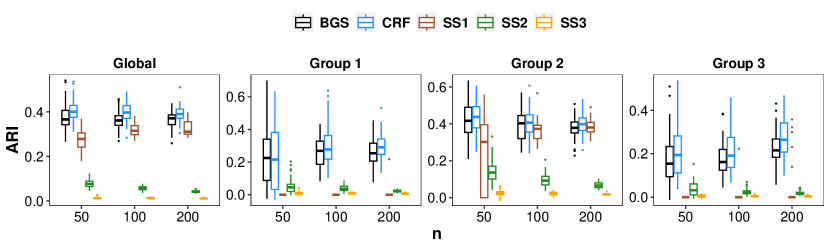
(a)

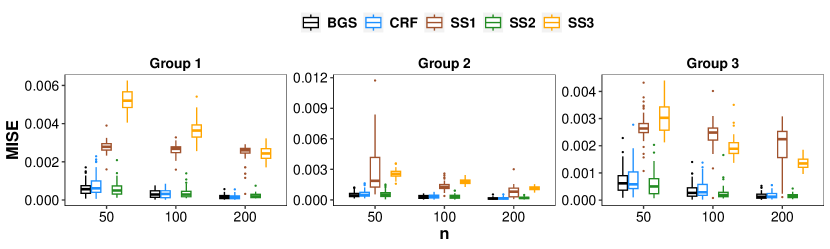
(b)

Figure 2: (a) Adjusted Rand indices of the estimated cluster labels (b) Mean integrated squared error of the estimated densities, when true means of the Gaussian mixture are $\mbox{\boldmath$\phi$}^{0}=(-3,-1,1,3)$. SS1, SS2, SS3 refer to the slice samplers with $\alpha_{0}$ chosen as 0.1, 1, 10 respectively. Boxplots show variation across 50 simulation replicates.

Figure 2 shows boxplots of the ARIs and the MISEs across 50 replicates. The generally low values of the ARIs are attributed to the high overlap between the adjacent Gaussian densities (refer also to §D.1 of the Supplement for the corresponding ARIs under a well-separated design, which shows values closer to 1). An overall decreasing trend in the MISE with increase in the sample size shows that posterior estimates of our algorithm are consistent. The clearly noticeable proximity in the ARI of cluster labels and the MISE of the density estimates obtained from BGS and CRF suggests that the two samplers provide very similar estimation performances. SS shows an overall worse performance, with the exception of its density estimates being along the lines of BGS and CRF when $\alpha_{0}$ is set as $1$, while when set as $0.1$, an improved accuracy in recovering the global cluster labels and the labels for group 2 is observed. Additional plots showing the estimated cluster labels and densities in one of the simulation replicates are provided in §D.2 of the Supplement.

4.2 Algorithmic Accuracy

In the following, we discuss mixing behavior of the sampled atoms and the estimated densities, and the computational efficiency of our algorithm. While CRF allows dynamic estimation of the number of clusters and samples atoms for each occupied cluster, BGS and SS on the contrary retain the unassigned clusters, the atoms corresponding to which are drawn independently from their prior. To bring all samplers on the same page, we define $\hat{L}=\min\{\hat{L}^{(m)}:m=1,2,\ldots,M\}$, where $\hat{L}^{(m)}$ denotes the number of estimated clusters by CRF in each posterior sample $m$, and retain the first $\hat{L}$ atoms from the posterior samples of CRF. We then extract $\hat{L}$ atoms from BGS and SS in decreasing order of their corresponding cluster occupancy to ensure that the atoms drawn from their prior are dismissed. Figure 3 shows boxplots of the effective sample sizes (ESS) of the occupied atoms and estimated densities, for each $n$ across 50 replicates. The plotted ESS of the density estimates is an average of element-wise ESS for the 100 grid points. Note that ESS can be higher than the number of MCMC samples in the presence of negative autocorrelation.

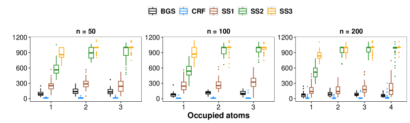
(a)

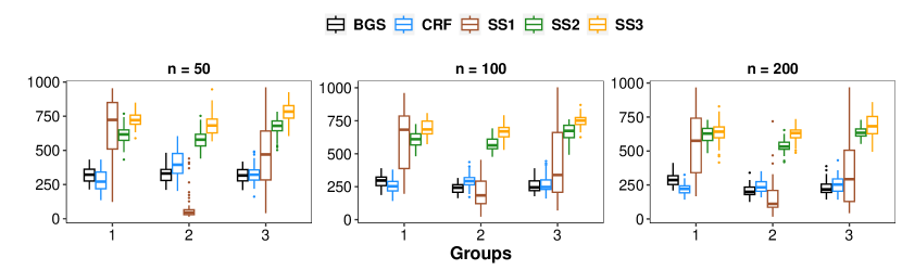
(b)

Figure 3: Effective sample sizes of (a) occupied atoms and (b) estimated densities, when true means of the Gaussian mixture are $\mbox{\boldmath$\phi$}^{0}=(-3,-1,1,3)$. SS1, SS2, SS3 refer to the slice samplers with $\alpha_{0}$ chosen as 0.1, 1, 10 respectively. Boxplots show variation across 50 simulation replicates.

While BGS and CRF have comparable ESS for the density estimates of each group, BGS has higher ESS than CRF for each of the atoms corresponding to the occupied clusters, for each $n$. The better mixing behavior of BGS can be attributed to its ability to update parameters in blocks as opposed to one-coordinate-at-a-time updates for parameters in CRF, and is consistent with the performance of the blocked Gibbs sampler for a DP (Ishwaran and James,, 2001). All three implementations of SS have considerably higher ESS for the occupied atoms. SS also has higher ESS for the estimated densities, except that for group 2 when $\alpha_{0}$ is set at $0.1$. This behavior is however not consistent with what is observed under well separated true clusters (in §D.1 of the Supplement), showing the lack of an interpretable pattern. Despite the mixing behavior, it is important to note that SS exhibits inadequate estimation performance under both overlapping and well separated true clusters, compared to the similar performances shown by BGS and CRF.

A remarkable gain in computational efficiency in using BGS as compared to CRF, is clearly evident in Figure 4 that shows boxplots of the average computation time per MCMC iteration for the two samplers across 50 replicates with increasing $n$. The code for implementing SS is found to have loops over the sample size requiring the need for optimization and is thereby omitted from our comparison of computational time. The scalability of BGS is ensured by its blocked parameter updates which factorize over the observations in each group, unlike the one-at-a-time updates of CRF that makes it suffer heavily when $n$ is large. Trajectories for the median of the average computation time show the stability of BGS with increasing $n$. The computation time can be further accelerated by trivial parallelization. Moreover, the posterior updates factorize over the $J$ groups, making the sampler suitable for applications with large sampler sizes as well as large number of groups.

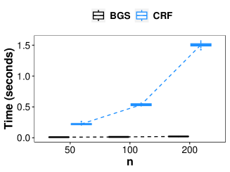
Figure 4: Average computation time (in seconds) per MCMC iteration, when true means of the Gaussian mixture are $\mbox{\boldmath$\phi$}^{0}=(-3,-1,1,3)$. Boxplots show variation across 50 simulation replicates, along with trajectories of the median time.

	Overlapping design			Well-separated design
	BGS	CRF	SS	BGS	CRF	SS
Clustering (ARI)	$\checkmark$	$\checkmark$	$\bm{\cdot}$	$\checkmark$	$\checkmark$	$\bm{\cdot}$
Density estimation (MISE)	$\checkmark$	$\checkmark$	$\ast$	$\checkmark$	$\checkmark$	$\ast$
Mixing (ESS)	$\checkmark$	$\bm{\cdot}$	$\bm{\cdot}$	$\checkmark$	$\ast$	$\bm{\cdot}$
Scalability (Computation time)	$\checkmark$	$\bm{\cdot}$	$-$	$\checkmark$	$\bm{\cdot}$	$-$

Table 1: Summary of the statistical and algorithmic performances of the three algorithms, as seen in our simulations. The symbols indicate the following performances: $\checkmark$ favorable, $\bm{\cdot}$ unfavorable or uninterpretable, $\ast$ favorable in some implementations, $-$ not included in the study.

Supplementary Materials

This supplement contains an enlisting of blocked parameter updates of the truncated HDP mixture model, derivation of the rejection sampler for the tilted gamma random variables, proof of auxiliary results and additional results from the simulation study of the main document.

Appendix A Blocked parameter updates of the truncated HDP mixture model

Let $F(\theta)$ have density $f(\cdot\mid\theta)$ and $H$ have density $h(\cdot)$. Likelihood and prior specifications from model (2.1), along with a Gamma $(a_{0},b_{0})$ prior on $\alpha_{0}$, are as follows,

$$\mbox{\boldmath$\beta$}\mid\gamma \sim\text{Dir}\left({\gamma}/{L},\ldots,{\gamma}/{L}\right) \phi_{k}\mid H \sim H$$

$$\mbox{\boldmath$\pi$}_{j}\mid\beta,\alpha_{0} \sim\text{Dir}\left(\alpha_{0}\mbox{\boldmath$\beta$}\right) z_{ji}\mid\mbox{\boldmath$\pi$}_{j} \sim\mbox{\boldmath$\pi$}_{j}$$

$$\alpha_{0}\mid a_{0},b_{0} \sim\text{Gamma }(a_{0},b_{0}) x_{ji}\mid z_{ji},\{\phi\}_{k=1}^{L} \sim F(\phi_{z_{ji}})$$

The full conditional distributions for the parameters are given by

1. Sampling $\phi$. For each $k=1,2,\ldots,L$,

   $$p(\phi_{k}\mid\bm{z},\mbox{\boldmath$\pi$},\mbox{\boldmath$\beta$},\alpha_{0}) \propto\ h(\phi_{k})\prod_{ji:z_{ji}=k}f(x_{ji}\mid\phi_{k})$$

   If $H$ is chosen conjugate to $F$, then we have independent conjugate updates for $\phi_{1},\phi_{2},\ldots,\phi_{L}$.

2. Sampling $\bm{z}$. For each $i=1,2,\ldots,n_{j}$ and $j=1,2,\ldots,J$,

   $$z_{ji}\mid\mbox{\boldmath$\phi$},\mbox{\boldmath$\pi$},\mbox{\boldmath$\beta$},\alpha_{0}\sim\mbox{\boldmath$\pi$}^{*}_{ji}$$

   where $\pi^{*}_{ji,k}=\frac{\pi_{jk}f(x_{ji}\mid\phi_{k})}{\sum_{l=1}^{L}\pi_{jl}f(x_{ji}\mid\phi_{l})}$ for each $k$.

3. Sampling $\pi$. For each $j=1,2,\ldots,J$,

   $$\mbox{\boldmath$\pi$}_{j}\mid\bm{z},\mbox{\boldmath$\phi$},\mbox{\boldmath$\beta$},\alpha_{0}\ \sim\ \text{Dir}(\mbox{\boldmath$n$}^{\prime}_{j}+\alpha_{0}\mbox{\boldmath$\beta$})$$

   where $\mbox{\boldmath$n$}^{\prime}_{j}=(n^{\prime}_{j1},n^{\prime}_{j2},\ldots,n^{\prime}_{jL}),\ n^{\prime}_{jk}=\sum_{i=1}^{n_{j}}\mathds{1}_{\{z_{ji}=k\}}$ for each $k$.

4. Sampling $\beta$.

   $$p(\mbox{\boldmath$\beta$}\mid\mbox{\boldmath$\phi$},\bm{z},\mbox{\boldmath$\pi$},\alpha_{0})\propto\ \Gamma(\alpha_{0})^{J}\prod_{k=1}^{L}\ \frac{1}{\Gamma(\alpha_{0}\beta_{k})^{J}}\ p_{k}^{\alpha_{0}\beta_{k}}\,\beta_{k}^{\,\frac{\gamma}{L}-1}\ \mathds{1}_{\left\{\mbox{\boldmath$\beta$}\in\mathcal{S}^{L-1}\right\}}$$

   where $p_{k}=\prod_{j=1}^{J}\pi_{jk}$ for each $k$ and $\mathcal{S}^{L-1}$ denotes the $L$-dimensional simplex.

5. Sampling $\alpha_{0}$.

   $$p(\alpha_{0}\mid\mbox{\boldmath$\phi$},\bm{z},\mbox{\boldmath$\pi$},\mbox{\boldmath$\beta$})\propto\alpha_{0}^{a_{0}-1}e^{-b_{0}\alpha_{0}}\ \frac{\Gamma(\alpha_{0})^{J}}{\prod_{k=1}^{L}\Gamma(\alpha_{0}\beta_{k})^{J}}\left(\prod_{k=1}^{L}p_{k}^{\beta_{k}}\right)^{\alpha_{0}}\mathds{1}_{\{\alpha_{0}>0\}}$$

Appendix B Rejection sampler for the tilted gamma random variables

In the following, we provide detailed derivation of the rejection sampler to get exact samples from the titled gamma density $f_{k}$, $k=1,2,\ldots,L$, given by

$$\begin{split}f_{k}(x)&\propto\frac{1}{\Gamma(x)^{J}}\ x^{\,A-1}\ e^{-B_{k}x}\ \mathds{1}_{\left\{x>0\right\}}\end{split}$$

where $\ A=\gamma/L$, $\ B_{k}=b_{0}-\text{log }p_{k}-\sum_{j=1}^{J}\text{log }u_{j}$. Let $\tilde{f}_{k}(x)=\frac{1}{\Gamma(x)^{J}}\ x^{\,A-1}\ e^{-B_{k}x}\ \mathds{1}_{\left\{x>0\right\}}$ and $C_{f_{k}}=\int_{0}^{\infty}\tilde{f}_{k}(x)\,dx$ denote the density upto constants and its normalizing constant, respectively. Note that $J\in\mathbb{N}$, $B_{k}\in{\mathbb{R}}$ and $A\in(0,1)$, since we are working with a finite truncation of an HDP mixture model by fixing the number of clusters ($L$) at a suitably chosen large number, as described in §2.3.

For developing a rejection sampler to get exact samples from our target density, $f_{k}$ with high acceptance rate, we require a sharp upper bound for $\tilde{f}_{k}$ that is convenient to sample from. We establish the log-concavity of $f_{k}$ in Lemma 2 and exploit it to get piece-wise tangent-line approximations, along with certain bounds of the gamma function, to develop the cover density separately for the cases when the parameter $B_{k}$ is positive and negative, such that the cover is tight and can be easily sampled from.

B.1 Rejection sampling algorithm

We briefly mention the steps of a rejection sampler for getting exact samples from $f_{k}$. Let $g_{k}=\tilde{g}_{k}/C_{g_{k}}$ be a density on $\mathbb{R}^{+}$ that can be sampled from and $\tilde{f}_{k}(x)\leq\tilde{g}_{k}(x)$ for all $x$ in the domain of $f_{k}$, then a rejection sampling algorithm proceeds as follows :

1. Draw $s\sim g_{k}$ and $u\sim\text{Uniform }(0,1)$ independently.

2. Accept $s$ as a sample from $f_{k}$ if $u\ \leq\ \tilde{f}_{k}(s)/\tilde{g}_{k}(s)$. Otherwise, return to Step 1.

B.2 Construction of the cover density

In this section, we describe the construction of the cover density, $g_{k}$ to get exact samples from our target density, $f_{k}$, $k\in\{1,2,\ldots,L\}$ using a rejection sampler as described in §B.1.

To that end, we first obtain an upper bound for $f_{k}$ using the following inequality (Laforgia and Natalini,, 2013) involving the gamma function on the interval $[1,\infty)$ in the form of a truncated gamma density. For $y>0$ and $\lambda\geq 0$,

$$e^{(1-\lambda)\psi(y+\lambda)}\leq\frac{\Gamma(y+1)}{\Gamma(y+\lambda)}\leq e^{(1-\lambda)\psi(y+1)}$$ (B.1)

with equalities occuring if and only if $\lambda=1$, where $\psi(x)=\frac{d}{dx}\,\text{log }\,\Gamma(x)$ denotes the digamma function.

Fixing $y=1$ and writing $\lambda=x-1$, the right-hand inequality in (B.1) implies the following for $x\geq 1$,

$$\frac{1}{\Gamma(x)}\leq e^{(2-x)\psi(2)}$$

which thereby gives

$$\tilde{f}_{k}(x)\ \leq\ e^{2J\psi(2)}\ x^{A-1}\ e^{-(J\psi(2)+B_{k})x},\quad x\geq 1.$$ (B.2)

It is important to note that depending on the value of $J$, the term $J\psi(2)+B_{k}$ may be negative when the parameter $B_{k}$ is negative, wherein the right-hand side of (B.2) does not lead to a valid density. This requires us to consider separate upper bounds for the cases when $B_{k}$ is positive and negative. Using (B.2) as an upper bound for $\tilde{f}_{k}$ in the case when $B_{k}>0$, we consider the following inequality (Li and Chen,, 2007) to upper bound $\tilde{f}_{k}$ when $B_{k}<0$.

For $x>1$,

$$\frac{x^{x-\gamma_{0}}}{e^{x-1}}<\Gamma(x)<\frac{x^{x-1/2}}{e^{x-1}}$$ (B.3)

with best possible constants $\gamma_{0}$ and $1/2$, where $\gamma_{0}=0.577215\ldots=-\psi(1)$ denotes the Euler–Mascheroni constant. For $0<x<1$, the left-hand inequality also holds, but the right-hand inequality is reversed.

Considering a positive constant $M$, the left-hand inequality in (B.3) implies for $x>M$,

$$\Gamma(x) >\frac{e^{(x-\gamma_{0})\,\text{log }\,x}}{e^{x-1}}>\frac{e^{(x-\gamma_{0})\,\text{log }\,M}}{e^{x-1}}$$

which gives an upper bound to $\tilde{f}_{k}$ as follows:

$$\tilde{f}_{k}(x)\ <\ e^{J\gamma_{0}\,\text{log }\,M-J}\ x^{A-1}\ e^{-\left(J\text{log }\,M-J+B_{k}\right)x},\quad x>M,$$ (B.4)

where we choose the constant $M$ in such a way that $J\,\text{log }\,M-J+B_{k}>0$, to get a valid truncated gamma density as an upper bound on the interval $(M,\infty)$. Our remaining task is to get an upper bound for $\tilde{f}_{k}$ on the bounded intervals $(0,1)$ and $(0,M]$ when $B_{k}$ is positive and negative respectively. We achieve this by using tangent lines of the logarithm of our target density $f_{k}$, exploiting the concavity of the log density.

Let us first consider the case when the parameter $B_{k}$ is positive. We note that $x^{\,A-1}\ e^{-B_{k}x}$ is decreasing and continuous on $(0,\infty)$ when $B_{k}>0$, while $1/\Gamma(x)^{J}$ is a continuous function increasing on $(0,3/2)$ and decreasing on $[3/2,\infty)$ implying that the mode of $f_{k}$ lies in $(0,3/2)$.

Let

$$\tilde{h}_{k}(x)=\text{log }\ \tilde{f}_{k}(x)=-J\,\text{log }\,\Gamma(x)+(A-1)\,\text{log }\,x-B_{k}x$$

denote the log density upto constants. Differentiating with respect to $x$, we have

$$\tilde{h}^{\prime}_{k}(x)=-J\,\psi(x)+\frac{(A-1)}{x}-B_{k}$$

Letting $m_{k0}$ denote the mode of $f_{k}$, which is obtained numerically by solving for $\tilde{h}^{\prime}_{k}(m_{k0})=0$, we fix two points $m_{k1}$ and $m_{k2}$ such that $m_{k1}=m_{k0}/2$ and $m_{k2}=(m_{k0}+3/2)/2$. Clearly, we have $0<m_{k1}<m_{k0}<m_{k2}<3/2$, which ensures that $\tilde{h}^{\prime}_{k}(m_{k1})>0$ and $\tilde{h}^{\prime}_{k}(m_{k2})<0$.

Equation of the tangent line of $\tilde{h}_{k}$ at the point $m_{ki}$, for $i=1,0,2,$ is given by

$$\nu_{ki}(x)=a_{ki}+\lambda_{ki}(x-m_{ki})$$ (B.5)

where $a_{ki}=\tilde{h}_{k}(m_{ki})$ and $\lambda_{ki}=\tilde{h}^{\prime}_{k}(m_{ki})$. Points of intersection of the tangent lines is given by

$$q_{ki}=\frac{a_{k0}-a_{ki}+m_{ki}\lambda_{ki}-m_{k0}\lambda_{k0}}{\lambda_{ki}-\lambda_{k0}},\quad\quad\text{for }i=1,2.$$ (B.6)

On the interval $(0,3/2]$, let

$$\nu_{k}(x):=\begin{cases}\nu_{k1}(x),&x\in(0,q_{k1}]\\ \nu_{k0}(x),&x\in(q_{k1},q_{k2}]\\ \nu_{k2}(x),&x\in(q_{k2},3/2]\end{cases}$$

Since $\tilde{h}_{k}$ is concave in nature and concave functions lie below their tangent lines, we have $\tilde{f}_{k}(x)\leq e^{\,\nu_{k}(x)}$ on $(0,3/2]$, which provides a piece-wise upper bound for $\tilde{f}_{k}$ on $(0,3/2]$. On the interval $(3/2,\infty)$, we shall use the bound obtained in (B.2). Thus, we have the following piece-wise upper bound for $\tilde{f}_{k}$ when $B_{k}>0$,

$$\tilde{f}_{k}(x)\ \leq\ \tilde{g}_{k}(x):=\begin{cases}e^{a_{k1}+\lambda_{k1}(x-m_{k1})},&x\in(0,q_{k1}]\\ e^{a_{k0}+\lambda_{k0}(x-m_{k0})},&x\in(q_{k1},q_{k2}]\\ e^{a_{k2}+\lambda_{k2}(x-m_{k2})},&x\in(q_{k2},3/2]\\ e^{2J\psi(2)}\ x^{A-1}\ e^{-(J\psi(2)+B_{k})x},&x\in(3/2,\infty)\end{cases}$$ (B.7)

For the case when the parameter ${B_{k}}$ is negative, on the bounded interval $(0,M]$, we numerically find the point at which $\tilde{f}_{k}$ is maximum and call it $m_{k0}$. If $m_{k0}<M$ i.e. if the mode lies in $(0,M]$, we fix two points $m_{k1}$ and $m_{k2}$ such that $m_{k1}=m_{k0}/2$ and $m_{k2}=(m_{k0}+M)/2$ which ensures $0<m_{k1}<m_{k0}<m_{k2}<M$ and hence $\tilde{h}^{\prime}_{k}(m_{k1})>0$ and $\tilde{h}^{\prime}_{k}(m_{k2})<0$. Otherwise, we fix $m_{k1}=M/4$, $m_{k0}=M/2$ and $m_{k2}=3M/4$ i.e. $m_{k1}$, $m_{k0}$ and $m_{k2}$ are three equidistant points in $(0,M]$. Equation of the tangent line $\nu_{ki}(x)$ of $\tilde{h}_{k}$ at the point $m_{ki}$, for $i=1,0,2,$ and the points of intersection, $q_{k1}$ and $q_{k2}$ of the tangent lines are obtained using (B.5) and (B.6). Again, using concavity of $\tilde{h}_{k}$ and the bound in (B.4), we have the following piece-wise upper bound for $\tilde{f}_{k}$ when $B_{k}<0$,

$$\tilde{f}_{k}(x)\ \leq\ \tilde{g}_{k}(x):=\begin{cases}e^{a_{k1}+\lambda_{k1}(x-m_{k1})},&x\in(0,q_{k1}]\\ e^{a_{k0}+\lambda_{k0}(x-m_{k0})},&x\in(q_{k1},q_{k2}]\\ e^{a_{k2}+\lambda_{k2}(x-m_{k2})},&x\in(q_{k2},M]\\ e^{J\gamma_{0}\,\text{log }\,M-J}\ x^{A-1}\ e^{-\left(J\text{log }\,M-J+B_{k}\right)x},&x\in(M,\infty)\end{cases}$$ (B.8)

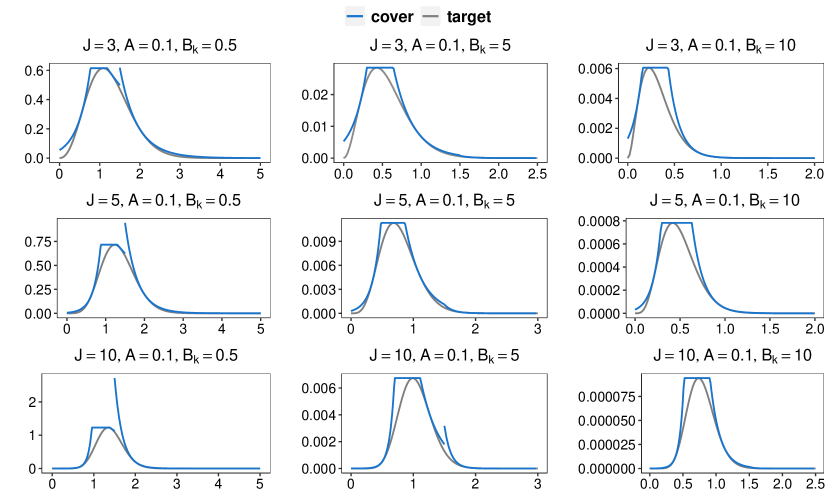
(a)

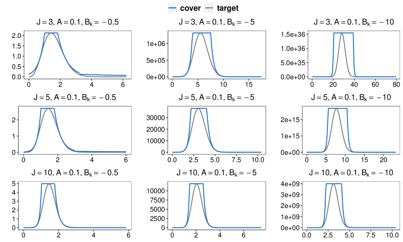
(b)

Figure 5: Plot of $\tilde{f}_{k}$ and the constructed cover $\tilde{g}_{k}$ for several choices of $J$, $A$ and $B_{k}$ when (a) $B_{k}>0$, (b) $B_{k}<0$.

To combine notations, let

$$\begin{split}\tilde{g}_{k,1}(x)&=e^{a_{k1}+\lambda_{k1}(x-m_{k1})}\ \mathds{1}_{\left\{x\in(0,q_{k1}]\right\}}\\ \tilde{g}_{k,2}(x)&=e^{a_{k0}+\lambda_{k0}(x-m_{k0})}\ \mathds{1}_{\left\{x\in(q_{k1},q_{k2}]\right\}}\\ \tilde{g}_{k,3}(x)&=e^{a_{k2}+\lambda_{k2}(x-m_{k2})}\ \mathds{1}_{\left\{x\in(q_{k2},q_{k3}]\right\}}\\ \tilde{g}_{k,4}(x)&=C_{k0}\ x^{A-1}\ e^{-B_{k0}x}\ \mathds{1}_{\left\{x\in(q_{k3},\infty)\right\}}\end{split}$$ (B.9)

where $C_{k0}=e^{2J\psi(2)}\mathds{1}_{\left\{B_{k}>0\right\}}+e^{J\gamma_{0}\text{log }M-J}\mathds{1}_{\left\{B_{k}<0\right\}}$, $B_{k0}=(J\psi(2)+B_{k})\mathds{1}_{\left\{B_{k}>0\right\}}+(J\text{log }\,M-J+B_{k})\mathds{1}_{\left\{B_{k}<0\right\}}$ and $q_{k3}=(3/2)\ \mathds{1}_{\left\{B_{k}>0\right\}}+M\ \mathds{1}_{\left\{B_{k}<0\right\}}$.

Let $\tilde{g}_{k}(x)=\tilde{g}_{k,1}(x)+\tilde{g}_{k,2}(x)+\tilde{g}_{k,3}(x)+\tilde{g}_{k,4}(x)$ and $g_{k}(x)=\tilde{g}_{k}(x)/C_{g_{k}}$ with $C_{g_{k}}=\int_{0}^{\infty}\tilde{g}_{k}(x)dx$. The normalizing constant $C_{g_{k}}$ is given by $C_{g_{k}}=C_{g_{k,1}}+C_{g_{k,2}}+C_{g_{k,3}}+C_{g_{k,4}}$,

$$C_{g_{k,1}} =\int_{0}^{q_{k1}}\tilde{g}_{k,1}(x)\ dx=\frac{e^{a_{k1}-m_{k1}\lambda_{k1}}}{\lambda_{k1}}\left(e^{q_{k1}\lambda_{k1}}-1\right)$$

$$C_{g_{k,2}} =\int_{q_{k1}}^{q_{k2}}\tilde{g}_{k,2}(x)\ dx=\begin{cases}\frac{e^{a_{k0}-m_{k0}\lambda_{k0}}}{\lambda_{k0}}\left(e^{q_{k2}\lambda_{k0}}-e^{q_{k1}\lambda_{k0}}\right),&\lambda_{k0}\neq 0\\ e^{a_{0}}\ (q_{k2}-q_{k1}),&\lambda_{k0}=0\end{cases}$$

$$C_{g_{k,3}} =\int_{q_{k2}}^{q_{k3}}\tilde{g}_{k,3}(x)\ dx=\frac{e^{a_{k2}-m_{k2}\lambda_{k2}}}{\lambda_{k2}}\left(e^{q_{k3}\lambda_{k2}}-e^{q_{k2}\lambda_{k2}}\right)$$

$$C_{g_{k,4}} =\int_{q_{k3}}^{\infty}\tilde{g}_{k,4}(x)\ dx=C_{k0}\ \frac{B_{k0}^{A}}{\Gamma(A)}\ \{1-F_{Y_{0}}(q_{k3})\}$$

where $Y_{0}$ denotes a random variable distributed as Gamma($A,B_{k0}$) with $F_{Y_{0}}(\cdot)$ denoting its cdf.

Then, the cover density $g_{k}$ can be written as a mixture of four densities,

$$g_{k}(x)=\frac{C_{g_{k,1}}}{C_{g_{k}}}\ g_{k,1}(x)+\frac{C_{g_{k,2}}}{C_{g_{k}}}\ g_{k,2}(x)+\frac{C_{g_{k,3}}}{C_{g_{k}}}\ g_{k,3}(x)+\frac{C_{g_{k,4}}}{C_{g_{k}}}\ g_{k,4}(x)$$

where

$$g_{k,1}(x) =\frac{\tilde{g}_{k,1}(x)}{C_{g_{k,1}}}=\frac{\lambda_{k1}}{e^{q_{k1}\lambda_{k1}}-1}\ e^{\lambda_{k1}x}\ \mathds{1}_{\{x\in(0,q_{k1}]\}}$$

$$g_{k,2}(x) =\frac{\tilde{g}_{k,2}(x)}{C_{g_{k,2}}}=\begin{cases}\frac{\lambda_{k0}}{e^{q_{k2}\lambda_{k0}}-e^{q_{k1}\lambda_{k0}}}\ e^{\lambda_{k0}x}\ \mathds{1}_{\{x\in(q_{k1},q_{k2}]\}},&\lambda_{k0}\neq 0\\ (q_{k2}-q_{k1})^{-1}\ \mathds{1}_{\{x\in(q_{k1},q_{k2}]\}},&\lambda_{k0}=0\end{cases}$$

$$g_{k,3}(x) =\frac{\tilde{g}_{k,3}(x)}{C_{g_{k,3}}}=\frac{\lambda_{k2}}{e^{q_{k3}\lambda_{k2}}-e^{q_{k2}\lambda_{k2}}}\ e^{\lambda_{k2}x}\ \mathds{1}_{\{x\in(q_{k2},q_{k3}]\}}$$

$$g_{k,4}(x) =\frac{\tilde{g}_{k,4}(x)}{C_{g_{k,4}}}=\frac{1}{1-F_{Y_{0}}(q_{k3})}\ \frac{B_{k0}^{A}}{\Gamma(A)}\ x^{A-1}\ e^{-B_{k0}x}\ \mathds{1}_{\{x\in(q_{k2},q_{k3}]\}}$$

B.3 Sampling from the cover density

In this section, we describe the procedure to get samples from the mixture density, $g_{k}$. For this purpose, let $w_{k,i}=C_{g_{k,i}}/C_{g_{k}}$, $i=1,2,3,4$ denote the mixture weights. Also, let $w_{k,0}=0$. A sample $s$ from $g_{k}$ is obtained as follows:

1. Generate a random variable $u\sim\text{Uniform }(0,1)$.

2. If $u\in\left[\sum_{j=0}^{i-1}w_{k,j},\sum_{j=0}^{i}w_{k,j}\right)$, then draw $s\sim g_{k,i}$, $i=1,2,3,4$.

We then proceed to describe the inverse cdf method to get samples from $g_{k,i}$, $i=1,2,3,4$.

The cdf of $g_{k,i}$, $i=1,2,3,4$ are given by

$$\begin{split}G_{k,1}(x)&=\frac{e^{\lambda_{k1}x}-1}{e^{\lambda_{k1}q_{k1}}-1}\mathds{1}_{\{x\in(0,q_{k1}]\}}\\ G_{k,2}(x)&=\begin{cases}\frac{e^{\lambda_{k0}x}-e^{\lambda_{k0}q_{k1}}}{e^{\lambda_{k0}q_{k2}}-e^{\lambda_{k0}q_{k1}}}\mathds{1}_{\{x\in(q_{k1},q_{k2}]\}},&\lambda_{k0}\neq 0\\ \frac{x-q_{k1}}{q_{k2}-q_{k1}}\mathds{1}_{\{x\in(q_{k1},q_{k2}]\}},&\lambda_{k0}=0\end{cases}\\ G_{k,3}(x)&=\frac{e^{\lambda_{k2}x}-e^{\lambda_{k2}q_{k2}}}{e^{\lambda_{k2}q_{k3}}-e^{\lambda_{k2}q_{k2}}}\mathds{1}_{\{x\in(q_{k2},q_{k3}]\}}\\ G_{k,4}(x)&=\frac{F_{Y_{0}}(x)-F_{Y_{0}}(q_{k3})}{1-F_{Y_{0}}(q_{k3})}\mathds{1}_{\{x\in(q_{k3},\infty)\}}\end{split}$$

and their respective inverses,

$$G_{k,1}^{-1}(u) =\lambda_{k1}^{-1}\ \text{log }\big{\{}u\,e^{\lambda_{k1}q_{k1}}+(1-u)\big{\}}$$

$$G_{k,2}^{-1}(u) =\begin{cases}\lambda_{k0}^{-1}\ \text{log }\left\{u\,e^{\lambda_{k0}q_{k2}}+(1-u)\,e^{\lambda_{k0}q_{k1}}\right\},&\lambda_{k0}\neq 0\\ {(x-q_{k1})}/{(q_{k2}-q_{k1})},&\lambda_{k0}=0\end{cases}$$

$$G_{k,3}^{-1}(u) =\lambda_{k2}^{-1}\ \text{log }\big{\{}u\,e^{\lambda_{k2}q_{k3}}+(1-u)\,e^{\lambda_{k2}q_{k2}}\big{\}}$$

Sampling from $\bm{g_{k,1},g_{k,2},g_{k,3}}$ : First, we note that when $m_{k0}$ is the mode of $f_{k}$, $\lambda_{k0}=0$ and $g_{k,2}$ is a $U(q_{k1},q_{k2})$ density which can be directly sampled from. To get a sample $s$ from $g_{k,i}$ when $\lambda_{k0}\neq 0$, $i=1,2,3$, which are exponential densities, the inverse cdf sampler proceeds as follows :

1. Draw $u\sim\text{Uniform }(0,1)$.

2. Set $s=G_{k,i}^{-1}(u)$.

Sampling from $\bm{g_{k,4}}$ : We note that $g_{k,4}$ is a gamma density with shape parameter, $A$ and rate parameter, $B_{k0}$ truncated on $(q_{k3},\infty)$. We can get a sample, $s$ from $g_{k,4}$ using an application of the inverse cdf sampler for truncated distributions, which proceeds as follows:

1. Draw $u\sim\text{Uniform }(F_{Y_{0}}(q_{k3}),1)$.

2. Set $s=F_{Y_{0}}^{-1}(u)$.

B.4 Empirical Illustrations

We investigate the performance of our proposed rejection sampler in terms of its acceptance probability. Figure 6 shows barplots of the acceptance probabilities over varying choices of parameters $J$, $A$ and $B_{k}$. When $B_{k}$ is positive, an acceptance rate of at least $70\%$ is observed for all choices of $J$ and $A$. A negative $B_{k}$ renders a slightly lower acceptance rate as compared to when it is positive. This is attributed to the right shifting of the mode of density for a negative $B_{k}$. Even so, we are able to get an acceptance rate of at least $40\%$ for all choices of $J$ and $A$. It is important to note that $B_{k}$ involves a large positive the term, $-\text{log }\ p_{k}$ where $p_{k}=\prod_{j=1}^{J}\pi_{jk}$ , $\pi_{jk}$ being the group-specific probabilities of each cluster, and hence the negative values it takes, remain small in magnitude.

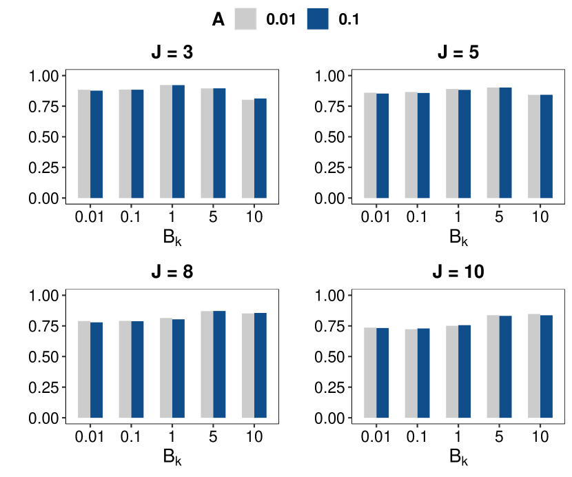
(a)

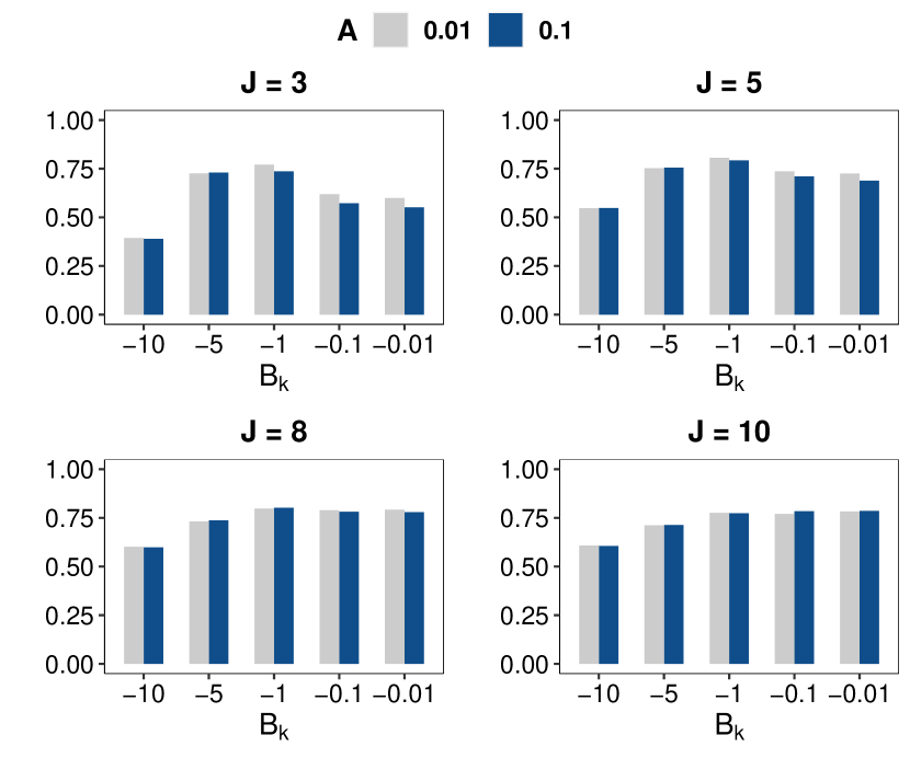
(b)

Figure 6: Barplots of acceptance probabilities of the rejection sampler over various choices of $J$, $A$ and $B_{k}$ when (a) $B_{k}>0$, (b) $B_{k}<0$.

Appendix C Proof of auxiliary results

Lemma 1.

A normalized vector $\bm{X}$ of jointly distributed random variables, $\bm{Y}=\left(Y_{1},Y_{2},\ldots,Y_{L}\right)$ with density $f_{\bm{Y}}$ on $(0,\infty)^{L}$, $L\in\mathbb{N}$, has joint density of the form,

$$f_{X_{1},X_{2},\ldots,X_{L-1}}(x_{1},x_{2},\ldots,x_{L-1})=\int_{0}^{\infty}y^{L-1}\,f_{\bm{Y}}(x_{1}y,x_{2}y,\ldots,x_{L}y)\ dy$$

with $x_{L}=1-\sum_{i=1}^{L-1}x_{i}$.

Proof. Kruijer et al., (2010) derived the density for the vector of normalized $\bm{Y}$ for the case when $Y_{1},Y_{2},\ldots,Y_{L}$ are independent random variables, with $Y_{i}$ having density $p_{i}$ on $(0,\infty)$, $i=1,2,\ldots,L$. We provide a straightforward extension of their proof to the case when $Y_{1},Y_{2},\ldots Y_{L}$ are dependent random variables.

We begin with writing

$$\bm{X}=(X_{1},X_{2},\ldots,X_{L})=\left(\frac{Y_{1}}{Y},\frac{Y_{2}}{Y},\ldots,\frac{Y_{L}}{Y}\right)$$

with $Y=\sum_{i=1}^{L}Y_{i}$. Then, for $(x_{1},x_{2},\ldots,x_{L})\in\mathcal{S}^{L-1}$, we have

$$P\left(X_{1}\leq x_{1},\ X_{2}\leq x_{2},\ldots,\ X_{L-1}\leq x_{L-1}\right)$$

$$=P\left(\frac{Y_{1}}{Y}\leq x_{1},\ \frac{Y_{2}}{Y}\leq x_{2},\ldots,\ \frac{Y_{L-1}}{Y}\leq x_{L-1}\right)$$

$$=\int_{0}^{\infty}\int_{0}^{x_{1}y}\int_{0}^{x_{2}y}\ldots\int_{0}^{x_{L-1}y}f_{\bm{Y}}\left(y_{1},y_{2},\ldots,y_{L-1},y-\sum_{i=1}^{L-1}y_{i}\right)\ dy_{L-1}\,dy_{L-2}\ldots dy_{1}\,dy$$

The joint density is then given by

$$f_{X_{1},X_{2},\ldots,X_{L-1}}(x_{1},x_{2},\ldots,x_{L-1})=\frac{\partial^{L-1}}{\partial x_{1}\partial x_{2}\ldots\partial x_{L-1}}\ P\left(X_{1}\leq x_{1},\ X_{2}\leq x_{2},\ldots,\ X_{L-1}\leq x_{L-1}\right)$$

Interchanging the $(L-1)$ derivatives and integrals, we have

$$f_{X_{1},X_{2},\ldots,X_{L-1}}(x_{1},x_{2},\ldots,x_{L-1})$$

$$=\int_{0}^{\infty}\frac{\partial}{\partial x_{1}}\int_{0}^{x_{1}y}\ldots\ \frac{\partial}{\partial x_{L-1}}\int_{0}^{x_{L-1}y}f_{\bm{Y}}\left(y_{1},y_{2},\ldots,y_{L-1},y-\sum_{i=1}^{L-1}y_{i}\right)\ dy_{L-1}\ldots\,dy_{1}\,dy$$

The proof follows by applying Leibniz integral rule for differentiation successively for $x_{L-1}$, $x_{L-2},\ldots,x_{1}$.

∎

Lemma 2.

For each $k=1,2,\ldots,L$, the density $f_{k}(x)\propto\frac{1}{\Gamma(x)^{J}}\ x^{A-1}\ e^{-B_{k}x}\ \mathds{1}_{\left\{x>0\right\}}$ is log-concave.

Proof. For any $k\in\{1,2,\ldots,L\}$, define the log density as

$$h_{k}(x)=\text{log }\,f_{k}(x)=-\text{log }\,C_{f_{k}}-J\,\text{log }\,\Gamma(x)+(A-1)\,\text{log }\,x-B_{k}x$$ (C.1)

where $C_{k}$ denotes the normalizing constant of $f_{k}$.

Differentiating (C.1) twice with respect to $x$, we have $h_{k}^{\prime\prime}(x)=-J\psi^{\prime}(x)-(A-1)/{x^{2}}$.

For proving concavity of $h_{k}$, it suffices to show that for all $x>0,\,J\geq 1,\,A\in(0,1)$,

$$x^{2}\,\psi^{\prime}(x)>\frac{1-A}{J}$$

Noting $(1-A)/J\in(0,1)$, we shall show that $x^{2}\psi^{\prime}(x)$ is a strictly increasing function of $x$ in $(0,\infty)$ and $\lim_{x\rightarrow 0^{+}}x^{2}\psi^{\prime}(x)=1$ which will complete our proof by implying that $x^{2}\psi^{\prime}(x)>1>{(1-A)}/{J}$.

For $x>0$, let

$$g(x)=x^{2}\psi^{\prime}(x)$$

Hence,

$$g^{\prime}(x)=x\,\{2\psi^{\prime}(x)+x\psi^{\prime\prime}(x)\}$$

For $x\in{\mathbb{R}}^{+}$ and $n\in{\mathbb{N}}$, integral representation of a polygamma function, $\psi^{(n)}(x)$ is as follows

$$\psi^{(n)}(x)=\frac{d^{n+1}}{dx^{n+1}}\,\text{log }\Gamma(x)=(-1)^{(n+1)}\int_{0}^{\infty}\frac{t^{n}}{1-e^{-t}}\ e^{-xt}\,dt$$ (C.2)

and we have the following recusion formula

$$\psi^{(n-1)}(x+1)=\psi^{(n-1)}(x)+(-1)^{(n-1)}\frac{(n-1)!}{x^{n}}$$ (C.3)

From (C.2) and (C.3), it follows that

$$\lim_{x\rightarrow 0^{+}}x^{n}\,\psi^{(n-1)}(x)=(-1)^{n}\,(n-1)!\ ,$$ (C.4)

details of which can be found in Yang, (2017) and Qi, (2015).

Putting $n=2$ in (C.4), we get

$$\lim_{x\rightarrow 0^{+}}g(x)=1$$ (C.5)

Next, for proving strict monotonicity of $g$, we put $n=2$ in (C.2) and integrate by parts to get

$$x\,\psi^{\prime\prime}(x) =-x\int_{0}^{\infty}\frac{t^{2}}{1-e^{-t}}\ e^{-xt}\,dt$$

$$=\int_{0}^{\infty}\frac{t^{2}}{1-e^{-t}}\ \frac{d}{dt}\left\{e^{-xt}\right\}\,dt$$

$$=-\int_{0}^{\infty}\frac{(2e^{t}-2-t)\,te^{t}}{(e^{t}-1)^{2}}\ e^{-xt}\ dt$$ (C.6)

Finally, putting $n=1$ in (C.2) and using (C), we have for all $x>0$,

$$2\,\psi^{\prime}(x)+x\,\psi^{\prime\prime}(x) =2\int_{0}^{\infty}\frac{t}{1-e^{-t}}\ e^{-xt}\,dt-\int_{0}^{\infty}\frac{(2e^{t}-2-t)\,te^{t}}{(e^{t}-1)^{2}}\ e^{-xt}\ dt$$

$$=\int_{0}^{\infty}\frac{t^{2}e^{t}}{(e^{t}-1)^{2}}\ e^{-xt}\ dt$$

$$>0$$

which thereby implies that $g^{\prime}(x)>0$ for all $x>0$ and combining with (C.5) completes our proof.

∎

Appendix D Additional Simulation Results

D.1 Performance under conjugate Gaussian mixture model with well separated clusters

We illustrate the statistical and algorithmic performances of our blocked Gibbs sampler under the well-separated design i.e. the Gaussian mixture model with true cluster means $\phi^{0}=(-6,-2,2,6)$, as discussed in §4

D.1.1 Statistical Accuracy

Figure 7 shows boxplots of the ARIs and the MISEs across 50 simulation replicates. BGS and CRF show similar accuracy in clustering and density estimation, as indicated by their high ARIs and low MISEs. SS shows an overall worse performance, with the exception of having improved density estimates for all choices of $n$ and all groups, when $\alpha_{0}$ is chosen as $1$.

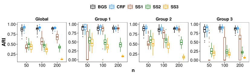
(a)

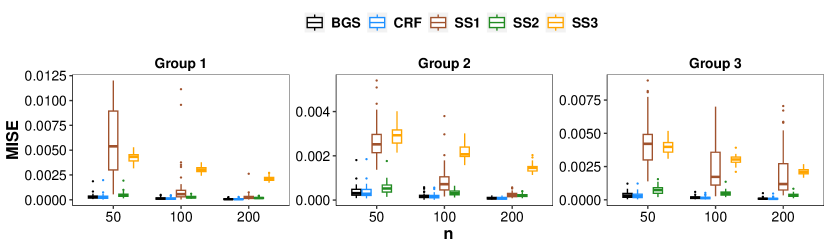
(b)

Figure 7: (a) Adjusted Rand indices of the estimated cluster labels (b) Mean integrated squared error of the estimated densities when true means of the Gaussian mixture are $\mbox{\boldmath$\phi$}^{0}=(-6,-2,2,6)$. SS1, SS2, SS3 refer to the slice samplers with $\alpha_{0}$ chosen as 0.1, 1, 10 respectively. Boxplots show variation across 50 simulation replicates.

D.1.2 Algorithmic accuracy

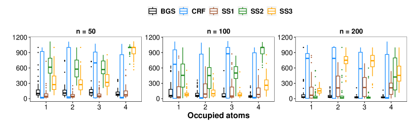
(a)

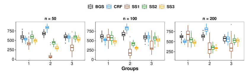
(b)

Figure 8: Effective sample sizes of (a) occupied atoms and (b) estimated densities, when true means of the Gaussian mixture are $\mbox{\boldmath$\phi$}^{0}=(-6,-2,2,6)$. SS1, SS2, SS3 refer to the slice samplers with $\alpha_{0}$ chosen as 0.1, 1, 10 respectively. Boxplots show variation across 50 simulation replicates.

Figure 8 shows boxplots of the effective sample sizes (ESS) of the occupied atoms and estimated densities, for each $n$ across 50 replicates, while Figure 9 shows boxplots of the average computation time per MCMC iteration. CRF is seen to have high variability in the ESS of occupied atoms across replicates, with the median being high in most of the cases. Under this design where the clusters are well separated, CRF often captures the true clusters quickly and samples the atoms independently for those clusters, consequently exhibiting a high ESS in such replicates, while having a low ESS in replicates when it fails to do so. BGS has similar ESS of occupied atoms, as seen under the overlapping design. The behavior of ESS corresponding to different implementations of SS in this regard, does not show any consistent pattern across varying $n$ and choices of $\alpha_{0}$. BGS and CRF show comparable ESS of the estimated densities, as seen in the case of overlapping clusters. All implementations of SS show similar behavior of ESS for groups 1 and 2, with lower values for group 2, in contrast to its overall high ESS under overlapping clusters. Trajectories for the median of the average computation time in Figure 9 is naturally similar to what is observed in the case of overlapping clusters and depicts the stability of BGS over increasing $n$.

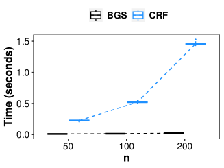
Figure 9: Average computation time (in seconds) per MCMC iteration, when true means of the Gaussian mixture are $\mbox{\boldmath$\phi$}^{0}=(-6,-2,2,6)$.. Boxplots show variation across 50 simulation replicates, along with trajectories of the median time.

D.2 Plots depicting estimation performance

In the following, we provide plots that depict the performance in clustering and density estimation, of BGS, CRF and the three implementations of SS in a single replicate of the simulation setting described in §4.

Figures 10 and 11 show the cluster labels estimated by the algorithms for all the groups along with the true labels for varying $n$, under overlapping and well separated clusters respectively. Figure 12 shows the estimated densities of the the three groups along with the true density, overlaid on the histogram of the observed data, for varying $n$.

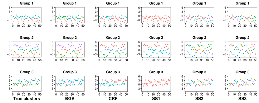
(a)

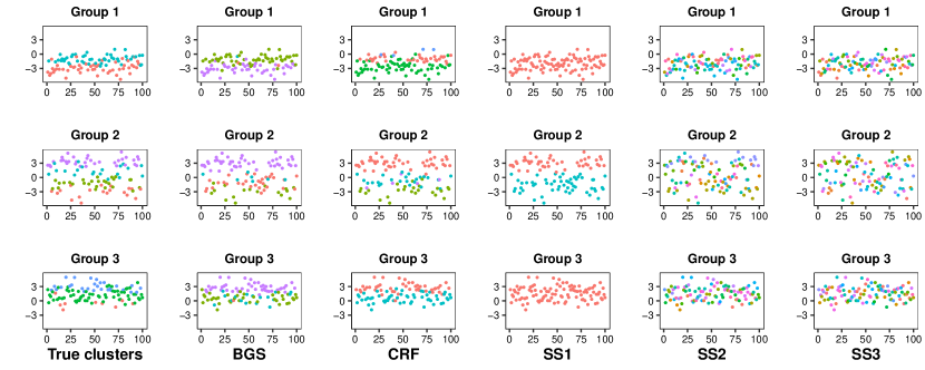
(b)

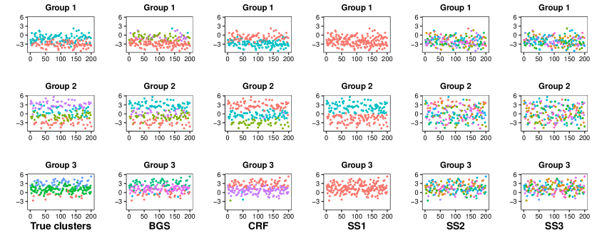
(c)

Figure 10: True and estimated cluster labels for (a) $n=50$ (b) $n=100$ (c) $n=200$, when true means of the Gaussian mixture are $\mbox{\boldmath$\phi$}^{0}=(-3,-1,1,3)$. SS1, SS2, SS3 refer to the slice samplers with $\alpha_{0}$ chosen as 0.1, 1, 10 respectively.

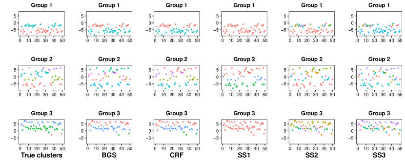
(a)

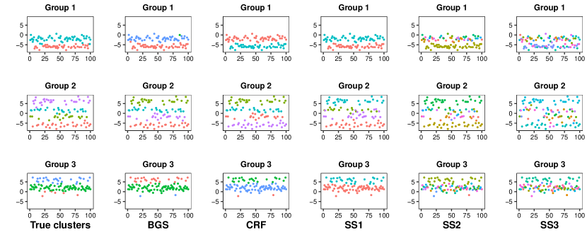
(b)

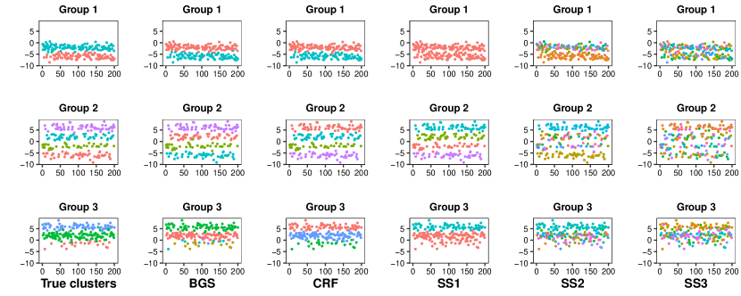
(c)

Figure 11: True and estimated cluster labels for (a) $n=50$ (b) $n=100$ (c) $n=200$, when true means of the Gaussian mixture are $\mbox{\boldmath$\phi$}^{0}=(-6,-2,2,6)$. SS1, SS2, SS3 refer to the slice samplers with $\alpha_{0}$ chosen as 0.1, 1, 10 respectively.

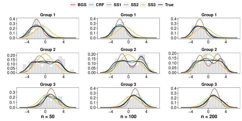
(a)

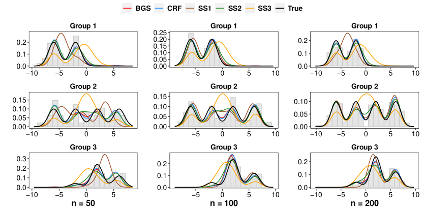
(b)

Figure 12: True and estimated densities overlaid on the histogram of the observed data, when true means of the Gaussian mixture are (a) $\mbox{\boldmath$\phi$}^{0}=(-3,-1,1,3)$ and (b) $\mbox{\boldmath$\phi$}^{0}=(-6,-2,2,6)$. SS1, SS2, SS3 refer to the slice samplers with $\alpha_{0}$ chosen as 0.1, 1, 10 respectively.

References

• Amini et al., (2019) Amini, A. A., Paez, M. S., Lin, L., and Razaee, Z. S. (2019). Exact slice sampler for Hierarchical Dirichlet Processes. ArXiv, abs/1903.08829.
• Asuncion et al., (2008) Asuncion, A., Smyth, P., and Welling, M. (2008). Asynchronous distributed learning of topic models. In Proceedings of the 21st International Conference on Neural Information Processing Systems, NIPS’08, page 81–88, Red Hook, NY, USA. Curran Associates Inc.
• Bryant and Sudderth, (2012) Bryant, M. and Sudderth, E. (2012). Truly nonparametric online variational inference for hierarchical dirichlet processes. In Advances in Neural Information Processing Systems, volume 25. Curran Associates, Inc.
• Canini et al., (2010) Canini, K. R., Shashkov, M. M., and Griffiths, T. L. (2010). Modeling Transfer Learning in Human Categorization with the Hierarchical Dirichlet Process. In Proceedings of the 27th International Conference on International Conference on Machine Learning, ICML’10, page 151–158, Madison, WI, USA. Omnipress.
• Chang and Fisher III, (2014) Chang, J. and Fisher III, J. W. (2014). Parallel Sampling of HDPs using Sub-Cluster Splits. In Ghahramani, Z., Welling, M., Cortes, C., Lawrence, N., and Weinberger, K., editors, Advances in Neural Information Processing Systems, volume 27. Curran Associates, Inc.
• Cowans, (2004) Cowans, P. J. (2004). Information Retrieval Using Hierarchical Dirichlet Processes. In Proceedings of the 27th Annual International ACM SIGIR Conference on Research and Development in Information Retrieval, SIGIR ’04, page 564–565, New York, NY, USA. Association for Computing Machinery.
• Dahl, (2006) Dahl, D. B. (2006). Model-Based Clustering for Expression Data via a Dirichlet Process Mixture Model, page 201–218. Cambridge University Press.
• Escobar and West, (1995) Escobar, M. D. and West, M. A. (1995). Bayesian Density Estimation and Inference Using Mixtures. Journal of the American Statistical Association, 90:577–588.
• Fox et al., (2011) Fox, E. B., Sudderth, E. B., Jordan, M. I., and Willsky, A. S. (2011). A sticky HDP-HMM with application to speaker diarization. The Annals of Applied Statistics, 5(2A):1020 – 1056.
• Gal and Ghahramani, (2014) Gal, Y. and Ghahramani, Z. (2014). Pitfalls in the use of parallel inference for the dirichlet process. In Xing, E. P. and Jebara, T., editors, Proceedings of the 31st International Conference on Machine Learning, volume 32 of Proceedings of Machine Learning Research, pages 208–216, Bejing, China. PMLR.
• Goldwater et al., (2006) Goldwater, S., Griffiths, T. L., and Johnson, M. (2006). Contextual dependencies in unsupervised word segmentation. In Proceedings of the 21st International Conference on Computational Linguistics and 44th Annual Meeting of the Association for Computational Linguistics, pages 673–680, Sydney, Australia. Association for Computational Linguistics.
• Hubert and Arabie, (1985) Hubert, L. J. and Arabie, P. (1985). Comparing partitions. Journal of Classification, 2:193–218.
• Ishwaran and James, (2001) Ishwaran, H. and James, L. F. (2001). Gibbs Sampling Methods for Stick-Breaking Priors. Journal of the American Statistical Association, 96:161 – 173.
• Ishwaran and Zarepour, (2002) Ishwaran, H. and Zarepour, M. (2002). Exact and approximate sum representations for the dirichlet process. Canadian Journal of Statistics, 30.
• Kim et al., (2016) Kim, Y., Chae, M., Jeong, K., Kang, B., and Chung, H. (2016). An Online Gibbs Sampler Algorithm for Hierarchical Dirichlet Processes Prior. In European Conference on Machine Learning and Knowledge Discovery in Databases - Volume 9851, ECML PKDD 2016, page 509–523, Berlin, Heidelberg. Springer-Verlag.
• Kruijer et al., (2010) Kruijer, W., Rousseau, J., and van der Vaart, A. (2010). Adaptive Bayesian density estimation with location-scale mixtures. Electronic Journal of Statistics, 4:1225–1257.
• Laforgia and Natalini, (2013) Laforgia, A. and Natalini, P. (2013). On Some Inequalities for the Gamma Function. Advances in Dynamical Systems and Applications, 8(2):261–267.
• Li and Chen, (2007) Li, X. and Chen, C.-P. (2007). Inequalities for the gamma function. Journal of Inequalities in Pure & Applied Mathematics [electronic only], 8.
• Qi, (2015) Qi, F. (2015). Complete monotonicity of a function involving the tri- and tetra-gamma functions. Proceedings of the Jangjeon Mathematical Society, 18(2):253–264.
• Rand, (1971) Rand, W. M. (1971). Objective Criteria for the Evaluation of Clustering Methods. Journal of the American Statistical Association, 66:846–850.
• Sohn and Xing, (2008) Sohn, K.-A. and Xing, E. P. (2008). A hierarchical dirichlet process mixture model for haplotype reconstruction from multi-population data. The Annals of Applied Statistics, 3:791–821.
• Teh et al., (2006) Teh, Y. W., Jordan, M. I., Beal, M. J., and Blei, D. M. (2006). Hierarchical Dirichlet Processes. Journal of the American Statistical Association, 101:1566 – 1581.
• Teh et al., (2007) Teh, Y. W., Kurihara, K., and Welling, M. (2007). Collapsed Variational Inference for HDP. In Proceedings of the 20th International Conference on Neural Information Processing Systems, NIPS’07, page 1481–1488, Red Hook, NY, USA. Curran Associates Inc.
• Wang and Blei, (2012) Wang, C. and Blei, D. M. (2012). A split-merge mcmc algorithm for the hierarchical dirichlet process. ArXiv, abs/1201.1657.
• Wang et al., (2011) Wang, C., Paisley, J., and Blei, D. M. (2011). Online variational inference for the hierarchical dirichlet process. In Proceedings of the Fourteenth International Conference on Artificial Intelligence and Statistics, volume 15 of Proceedings of Machine Learning Research, pages 752–760, Fort Lauderdale, FL, USA. PMLR.
• Williamson et al., (2013) Williamson, S., Dubey, A., and Xing, E. (2013). Parallel Markov chain Monte Carlo for nonparametric mixture models. In Proceedings of the 30th International Conference on Machine Learning, volume 28 of Proceedings of Machine Learning Research, pages 98–106, Atlanta, Georgia, USA. PMLR.
• Wu, (2020) Wu, P. (2020). Comparison of Different Hierarchical Dirichlet Process Implementations. Master’s thesis, University of California, Los Angeles.
• Yang, (2017) Yang, Z.-H. (2017). Some properties of the divided difference of psi and polygamma functions. Journal of Mathematical Analysis and Applications, 455:761–777.