Quark Chromo-Electric Dipole Moment Operator on the Lattice

Abstract

We present a lattice QCD study of the contribution of the isovector quark chromo-electric dipole moment (qcEDM) operator to the nucleon electric dipole moments (nEDM). The calculation was carried out on four 2+1+1-flavor of highly improved staggered quark (HISQ) ensembles using Wilson-clover quarks to construct correlation functions. This clover-on-HISQ formulation is not fully $O(a)$ improved, and gives rise to additional systematics over and above those due to removing excited state contributions to getting ground-state matrix elements, and the final chiral and continuum extrapolations to get the physical result. We use the non-singlet axial Ward identity including corrections up to $O(a)$ to show how to control the power-divergent mixing of the isovector qcEDM operator with the lower dimensional pseudoscalar operator. The residual corrections are observed to give rise to $O(25\%)$ violations in relations arising from the axial Ward identity. We devise three methods attempting to control the resulting uncertainty in the CP violating form factor; each of these, however, can have large $O(a^{2})$ corrections. Preliminary results for the nEDM due to qcEDM are presented choosing the method giving the most uniform behavior.

I Introduction

The observation of permanent electric dipole moments (EDMs) in nondegenerate systems requires the simultaneous breaking of parity (P) and time reversal (T), or, equivalently, the combination of charge conjugation and parity (CP) [1]. Given the smallness of CP-violating ($\cancel{\text{CP}}$) contributions induced by quark mixing described by the Cabibbo-Kobayashi-Maskawa (CKM) matrix in the Standard Model (SM) [2], CP-violation in nucleon, nuclear, and atomic/molecular [3, 4, 5, 6, 7, 8, 9] systems provide very strong constraints on the SM $\Theta$-term (currently constrained at the level of $\Theta\sim 10^{-10}$) and new sources of CP violation arising from physics beyond the Standard Model (BSM) [10, 11].

New $\cancel{\text{CP}}$ interactions are ubiquitous in BSM models and may play a key role in relatively low-scale baryogenesis mechanisms, such as electroweak baryogenesis (see [12] and references therein). Probing them through hadronic electric dipole moments (EDMs), however, requires including possible large corrections due to the strong interactions between quark and gluon fields. These are analyzed using low-energy effective operators and require nonperturbative treatment. For hadronic systems such as the neutron, lattice QCD (LQCD) has emerged as the tool of choice to compute the contribution of these $\cancel{\text{CP}}$ operators to the EDMs. Furthermore, it has been shown quantitatively that improving the precision of these hadronic matrix elements will drastically improve the constraints that EDMs provide on $\cancel{\text{CP}}$ BSM interactions of the Higgs particle [13, 14, 15].

The outline of this paper is as follows. In Section I.1, we review the need for new sources of $\cancel{\text{CP}}$. The parameterization of $\cancel{\text{CP}}$ operators at the hadronic scale using effective field theory methods is presented in Section I.2. In this study, we only calculate the EDMs of the neutron (nEDM) and proton (pEDM) induced by the isovector component of the quark chromo-electric dipole moment (qcEDM). The decomposition of the matrix elements of $\cancel{\text{CP}}$ operators within ground state nucleons into vector form-factors of the nucleons, and the phase conventions are given in Section II. In Section III, we describe the method for calculating these form factors on the lattice. The use of the axial Ward identity to control the power law divergence due to mixing with the lower dimension pseudoscalar operator is described in Section IV and some preliminary numerical results are presented in Section V. In Section VI, we discuss the multiplicative renormalization of the qcEDM operator and the connection to the $\overline{\rm MS}$ scheme. Our conclusions are given in Section VII. Four appendices present technical details: Appendix A discusses the nonsinglet Ward Identity, Appendix B provides a complete list of dimension-5 CPV operators, Appendix C details the nonperturbative procedure for the extraction of the coefficient, $K_{X1}$, needed to control the power-divergent mixing of the qcEDM and pseudoscalar operators, and Appendix D gives the chiral perturbation theory determination of the chiral phase $\alpha_{N}$ for the nucleon.

I.1 Baryogenesis and the need for new sources of CP violation

The observed universe has $6.1^{+0.3}_{-0.2}\times 10^{-10}$ baryons for every black body photon [16], whereas in a baryon symmetric universe, we expect no more that about $10^{-20}$ baryons and antibaryons for every photon [17]. It is difficult to include such a large excess of baryons as an initial condition in an inflationary cosmological scenario [18]. The way out of the impasse lies in generating the baryon excess (baryogenesis) dynamically during the evolution of the universe.

In the early history of the universe, if the matter-antimatter asymmetry was generated post inflation and reheating, then one has to satisfy Sakharov’s three necessary conditions [19]: the process has to violate baryon number, evolution has to occur out of equilibrium, and CP (or, equivalently, time reversal invariance if CPT remains unbroken) has to be violated.

To probe sources of $\cancel{\text{CP}}$, a very promising approach is to search for static EDMs of elementary particles, atoms and nondegenerate states of molecules, all of which are necessarily proportional to their spin. Since under time-reversal, the direction of spin reverses but the electric dipole moment does not, a nonzero measurement would imply T, or equivalently CP, violation. Of the elementary particles, atoms and nuclei that are being investigated, nEDM and pEDM are the cleanest to analyze using lattice QCD.

CP violation exists in the electroweak sector of the SM of particle interactions due to a phase in the CKM quark mixing matrix [2], and possibly by a similar phase in the leptonic sector [20, 21], given that the neutrinos have mass and mix. The contribution of the $\cancel{\text{CP}}$ phase in the CKM quark mixing matrix [2] to nEDM is $O(10^{-32})$ e-cm [22], much smaller than the current experimental bound $d_{n}<1.8\times 10^{-26}$ e-cm (90% CL) [3]. This $\cancel{\text{CP}}$ is too small to explain baryogenesis [23, 24, 25, 26, 27, 28]. Similarly, $\cancel{\text{CP}}$ due to a possible topological term [29] is unlikely to lead to appreciable baryon asymmetry [30]. For baryogenesis, BSM $\cancel{\text{CP}}$ would, therefore, need to have played a major role. Most extensions of the SM have new sources of $\cancel{\text{CP}}$. Each of these contributes to the nEDM and for some models it can be as large as $10^{-26}$ e-cm. Planned experiments aim to reach a sensitivity of $d_{n}\sim 3\times 10^{-28}$ e-cm [11].

In order to connect the reduction in the upper bounds or actual values from EDM searches to new sources of $\cancel{\text{CP}}$ and models of baryogenesis, robust calculations of the hadronic EDMs induced by low-energy effective quark and gluon operators are needed. Lattice QCD offers the most promising method with control over all uncertainties to provide the matrix elements of novel $\cancel{\text{CP}}$ operators between nucleon states that are needed to connect the experimental bound (or value!) of the EDMs to the CP violating couplings in a given BSM theory. Here, we present the calculation of the isovector part of the qcEDM operator.

I.2 CP violation at low energy up to dimension-five

At the hadronic scale (${}\lesssim 2$ GeV), the effects of BSM theories that involve heavy degrees of freedom at mass scales greater than the weak scale, $\Lambda>M_{W}$, can be described in terms of effective local operators composed of quarks and gluons. Using effective field theory techniques, one can organize all such $\cancel{\text{CP}}$ interactions based on symmetry and dimension. In general, operators with higher dimension are suppressed by increasing inverse powers of $\Lambda$. The couplings associated with these low-energy operators encode information about the BSM model at $\Lambda\sim$ TeV scale with the renormalization group providing their evolution from $\Lambda$ to the hadronic scale. The nEDM induced by any $\cancel{\text{CP}}$ interaction can be obtained from the $\cancel{\text{CP}}$ form factor $F_{3}$ of the electromagnetic current, $J_{\mu}^{\rm EM}$, within the nucleon state, as discussed below.

At dimension five and lower, only three $\cancel{\text{CP}}$ local operators arise:

$${\cal L}_{\rm QCD}\mathbin{{\longrightarrow}}{\cal L}_{\rm QCD}^{\cancel{\text{CP}}}={\cal L}_{\rm QCD}+\frac{i}{32\pi^{2}}\Theta\ G_{\mu\nu}{\tilde{G}_{\mu\nu}}$$

$$\!{}-\left.\frac{i}{2}\sum_{q}d_{q}\ \overline{q}\sigma^{\mu\nu}{\tilde{F}_{\mu\nu}}q\right.-\left.\frac{i}{2}\sum_{q}d_{q}\ \overline{q}\sigma^{\mu\nu}{\tilde{G}_{\mu\nu}}q\right.\,,$$ (1)

where $\tilde{F}^{\mu\nu}=\epsilon^{\mu\nu\alpha\beta}F_{\alpha\beta}/2$ is the dual of the electromagnetic field-strength tensor, $\tilde{G}^{\mu\nu}=\epsilon^{\mu\nu\alpha\beta}G_{\alpha\beta}/2$ is the dual of the QCD field-strength tensor, and $\sigma_{\mu\nu}=(i/2)[\gamma_{\mu},\gamma_{\nu}]$. These three $\cancel{\text{CP}}$ opertors are the $d=4$ $\Theta$-term and the $d=5$ quark EDM (qEDM) and the qcEDM with dimensionful coefficients $d_{q}$ and $\tilde{d}_{q}$, respectively. Recent work on the dimension six gluonic operator (the Weinberg operator) [31] can be found in Refs. [32, 33], while there has been less work done on the $\cancel{\text{CP}}$ four-fermion operators [34, 35].

To the lowest order, the calculation of the qEDM is special; it reduces to the calculation of the flavor diagonal tensor charges of the neutron. The methodology for this calculation, including disconnected contributions from up, down, strange, and charm quark loops, is mature and first lattice results obtained by us are given in Ref. [36] and phenomenological consequences for a particular BSM theory (Split SUSY) were analyzed in Ref. [37]. These results were updated in Ref. [38], and the status of various lattice calculations are reviewed by the Flavor Lattice Averaging Group (FLAG) in Refs. [39, 40].

The calculation of nEDM induced by the $\Theta$-term requires the matrix elements of the product of the gluonic operator with the $J_{\mu}^{\rm EM}$ within the ground state of the nucleon. While the computation is only slightly more expensive than of the 3-point function with just $J_{\mu}^{\rm EM}$, the calculation is still not under control due to both statistical errors and lack of a clear methodology to fully remove excited state contributions (ESC), especially from the low-lying tower of nucleon-pion states. Recent progress has been reported in Refs. [41, 42, 43, 44, 45].

Note that because of the anomaly in the axial Ward identity, the $\Theta$-term can be rotated into a pseudoscalar mass term $im_{\ast}({\Theta})\sum_{q}\overline{q}\gamma_{5}q$ under a chiral transformation [46], and conversely, any phase arising in the determinant of the quark mass-matrix can be traded for $\Theta$. Since the nonanomalous axial Ward identities allow us to remove the rest of the phases in the mass-matrix, we will, henceforth, treat all quark masses as real. The $\Theta$-term is part of the SM, but is usually neglected under the assumption that some form of a Peccei-Quinn mechanism that promotes $\Theta$ to a dynamical field relaxes the minimum of its effective action to $\Theta=0$ [47] in the absence of other $\cancel{\text{CP}}$ sources in the action. It is, however, important to note that in the presence of other $\cancel{\text{CP}}$ operators from BSM, the minimum, called $\Theta_{\rm induced}$ [48], of this effective potential is, in general, shifted by the disconnected contributions, i.e., those in which the quark fields in the operator are contracted to form a quark loop.

Furthermore, the contribution to the minimum, induced by the qEDM and qcEDM operators vanishes for the isovector combination in an isospin-symmetric theory. We, therefore, do not consider this effect here as we present only the connected contributions of the qcEDM operator.

Calculations of even the bare qcEDM operator are the most challenging computationally of the three $D\leq 5$ operators. Furthermore, to get finite results in the continuum limit, one must resolve its divergent mixing with the $D=3$ pseudoscalar operator $i\sum_{q}\bar{q}\gamma_{5}q$ as discussed in Refs. [49, 33, 50]. Our analysis starts with the Hermitian flavor-diagonal and isovector qcEDM operators defined as

$$C^{(q)} \equiv-\frac{i}{2}\,\overline{q}\sigma_{\mu\nu}\tilde{G}_{\mu\nu}q\ =\ \frac{i}{2}\,\overline{q}\sigma_{\mu\nu}\gamma_{5}G_{\mu\nu}q$$

$$C^{(a)} \equiv i\,\overline{\psi}\sigma_{\mu\nu}\gamma_{5}G_{\mu\nu}T^{a}\psi~{},$$ (2)

where $q$ denotes the quark field of a given flavor while $\psi$ denotes the $SU(N_{f})$ multiplet in the fundamental representation and $T^{a}$ represents the generic hermitian $SU(N_{f})$ generator, normalized as $\mathop{\rm Tr}\nolimits[(T^{a})^{2}]=\frac{1}{2}$.

To the lowest order in $\tilde{d}_{q}$, the nEDM induced by the qcEDM operator requires calculating

$$\langle n\mid J^{\rm EM}_{\mu}\mid n\rangle\Big{|}_{\not{{\rm CP}}}^{\rm qcEDM}\!\!\!\!\! =\langle n|J^{\rm EM}_{\mu}\ \times{}$$

$$\int d^{4}x\ (-\frac{i}{2})\sum_{q\in u,d,s}\tilde{d}_{q}\,\bar{q}\sigma_{\alpha\beta}q\ {\tilde{G}}^{\alpha\beta}|n\rangle\,,$$ (3)

where effects of the heavier quarks are ignored. This is a 4-point function–the volume integral of the qcEDM operator correlated with the electromagnetic current inserted on each time slice between the nucleon source and sink. This can be calculated in two ways using lattice QCD: directly as a 4-point function [51] or using the Schwinger source method discussed in [52, 53]. Here, we continue to develop the latter.

In the Schwinger source method, the qcEDM operator, a bilinear in the quark fields, is added as a source term to the QCD action. Correlation functions with its insertion can then be calculated by taking derivatives with respect to its coupling $\tilde{d}_{q}$. We divide this calculation into two steps: first, regular, $P$, and modified, $P_{\epsilon}$, propagators are calculated by inverting the Dirac operator without and with the qcEDM term. Second, these two propagators are used to construct the three-point function with the insertion of the vector current between nucleon states, i.e., the quark-line diagrams in Figs. 1 and 2.

Since the modified propagator inserts arbitrary powers of the qcEDM operator, one gets uncontrolled divergences if the continuum limit is taken holding $\tilde{d}_{q}$ fixed. We, therefore, scale $\tilde{d}_{q}$ appropriately to keep the contribution in the linear regime as we take the continuum limit. For convenience, we will express most quantities in terms of the dimensionless ratios

$$\epsilon_{{q}}\equiv-\frac{2\tilde{d}_{q}}{ar}\,\qquad q=u,d,s,$$ (4)

where $a$ is the lattice spacing and $r$ is a dimensionless parameter in the Wilson discretization of the fermion action, as described in Eq. 16.

II Form Factors decomposition of the Electromagnetic Current in Presence of CP violation

The nucleon matrix element of the electromagnetic current $J^{\rm EM}_{\mu}=\sum_{q}e_{q}\,\bar{q}\gamma_{\mu}q$, where $e_{q}$ is the charge of the quark, in the presence of parity violating interactions can be parameterized in terms of the most general set of form factors consistent with the symmetries of the theory. Working in the Euclidean space we have:

$$\langle N(p^{\prime})|J_{\mu}^{\rm EM}|N(p)\rangle =\overline{u}_{N}(p^{\prime})\big{[}\gamma_{\mu}F_{1}+{}\hskip 43.36464pt$$

$$\frac{1}{2M_{N}}\sigma_{\mu\nu}q_{\nu}\left(F_{2}-iF_{3}\gamma_{5}\right)+{}$$

$$\frac{F_{A}}{M_{N}^{2}}(\not{q}q_{\mu}-q^{2}\gamma_{\mu})\gamma_{5}~{}\big{]}u_{N}(p)\ ,$$ (5)

where $M_{N}$ is the neutron mass, $q=p^{\prime}-p$ is the momentum carried by the electromagnetic current, $\sigma_{\mu\nu}=(i/2)[\gamma_{\mu},\gamma_{\nu}]$, and $u_{N}(p)$ represents the free neutron spinor of momentum $p$ obeying $(i\not{p}+M_{N})u_{N}(p)=0$. $F_{1}$ and $F_{2}$ are the Dirac and Pauli form factors, in terms of which the Sachs electric and magnetic form factors are $G_{E}=F_{1}-(q^{2}/4M_{N}^{2})F_{2}$ and $G_{M}=F_{1}+F_{2}$, respectively. The anapole form factor $F_{A}$ and the electric dipole form factor $F_{3}$ violate parity P; and $F_{3}$ violates CP as well. The zero $q^{2}$ limit of these form factors gives the charges and dipole moments: the electric charge is $G_{E}(0)=F_{1}(0)$ and the magnetic dipole moment is $F_{2}(0)/2M_{N}$. The nEDM is obtained from $F_{3}(q^{2})$ as follows:

$$d_{n}=\lim_{q^{2}\to 0}\frac{F_{3}(q^{2})}{2M_{N}}~{}.$$ (6)

In what follows we will specialize to the isovector qcEDM $\tilde{d}\equiv\tilde{d}_{u}=-\tilde{d}_{d}$ (implying $\epsilon\equiv\epsilon_{u}=-\epsilon_{d}$), which corresponds to

$${\cal L}^{\cancel{\text{CP}}}=\tilde{d}\Big{(}C^{(u)}-C^{(d)}\Big{)}=\tilde{d}\,C^{(3)}=-\frac{ar\epsilon}{2}\,C^{(3)}\,.$$ (7)

All lattice results will be presented in terms of the dimensionless coefficient $X_{c}$ relating the nEDM to $\tilde{d}\equiv\tilde{d}_{u}$,

$$d_{n}=X_{c}\ \tilde{d}=-X_{c}\frac{ar}{2}\epsilon~{}.$$ (8)

where

$$X_{c}=\frac{-F_{3}(q^{2}=0)}{ar\epsilon M_{N}}.$$ (9)

with $r=1$ in the Wilson-clover action we use.

Subtleties related to the phase convention for the neutron interpolating field in presence of $\cancel{\text{CP}}$ have been discussed and clarified in Refs. [54, 51, 44]. For completeness, we discuss the relevant issues here from a slightly different perspective.

The usual representation of the free Dirac Equation $(i\not{p}+m)u^{s}(p)=0$ is invariant under the Lorentz transformation and the discrete symmetries C, P, and T with the familiar expressions for their generators. The asymptotic in and out states of an interacting field theory are free states, and hence obey the symmetries of the free theory even when the underlying theory does not preserve these. There is, however, an important distinction between the cases when the full theory preserves the symmetry and when the symmetries only appear asymptotically.

There is a freedom of representation in the free Dirac equation: an arbitrary transformation $u\to Xu$, $\Gamma\to\Gamma_{X}\equiv X\Gamma X^{-1}$, with X a fixed arbitrary matrix and $\Gamma$ an element of the Clifford algebra of the $\gamma$-matrices, preserves the form of the free Dirac equation; but all the symmetry generators need to be written using $\Gamma_{X}$ instead of $\Gamma$. In a theory where the symmetries are preserved, the same generators can be chosen to implement the symmetries on all states, and, hence, interpolating operators can be chosen so that $X=1$ for all asymptotic fermionic states without solving for the dynamics. In a general theory, however, the symmetry operations on each asymptotic state that an interpolating operator couples to will have a different $X$, and the interpolating operators cannot be chosen to make all of them unity.

In particular, consider an interpolating field that produces asymptotic states described by the conventional $u^{s}$ spinors when parity is conserved. When parity is broken, the asymptotic states that this operator couples to will instead be solutions of the rotated equation $(i\not{p}+m)\exp(i\alpha\gamma_{5})u^{s}=0$, for some a priori unknown $\alpha$. To determine the value of this constant, one can study the propagator, i.e., two-point function of the interpolating field $N$. Because of Lorentz symmetry, a spin-$\frac{1}{2}$ field $N$ will have a propagator given by

$$\langle TN\bar{N}\rangle =\hskip 164.77771pt$$

$$e^{i\alpha(p^{2})\gamma_{5}}\left[iA(p^{2})\not{p}+\Sigma(p^{2})\right]^{-1}e^{i\alpha^{*}(p^{2})\gamma_{5}}\,.$$ (10)

The asymptotic large-time behavior of this propagator is given by the residues of its poles. The residue of the pole at $p^{2}=-M_{N}^{2}$ (i.e., $p^{2}_{\rm Minkowski}=M_{N}^{2}$) is given by

$$Ze^{i\alpha(-m_{N}^{2})\gamma_{5}}(-i\not{p}+m)e^{i\alpha^{*}(-m_{N}^{2})\gamma_{5}} =\hskip 43.36464pt$$

$$Z\sum_{s}\tilde{u}^{s}(p)\overline{\tilde{u}^{s}}(p)\,,$$ (11)

where

$$\tilde{u}^{s}(p)\equiv e^{i\alpha(-m_{N}^{2})\gamma_{5}}u^{s}(p)$$ (12)

is the spinor in the rotated representation.

After obtaining $\alpha_{N}\equiv\alpha(-M_{N}^{2})$ in this way, one has two options: First, continue to use this representation cognizant of the fact that this leads to a ‘rotated’ Dirac equation, and hence all the symmetry operators and projectors need to be written using the rotated $\gamma$-matrices. In particular, in the coefficients of the $F_{2}$ and $F_{3}$ form factors in Eq. 5 we need to replace $[\gamma_{\mu},\gamma_{\nu}]$ by $e^{i\alpha_{N}^{*}\gamma_{5}}[\gamma_{\mu},\gamma_{\nu}]e^{i\alpha_{N}\gamma_{5}}$. We follow this strategy since we do not calculate the full $4\times 4$ Dirac structure of the three-point function needed for the second option.

Conceptually, the much simpler alternative is to rotate the interpolating field $N$ to $N_{\alpha_{N}}\equiv e^{-i\alpha_{N}\gamma_{5}}N$, or equivalently, rotate all the correlation functions constructed from $N$ as

$$\langle N{\cal O}\bar{N}\rangle \to\langle N_{\alpha_{N}}{\cal O}\bar{N}_{\alpha_{N}}\rangle$$

$$=e^{-i\alpha_{N}\gamma_{5}}\langle N{\cal O}\bar{N}\rangle e^{-i\alpha_{N}^{*}\gamma_{5}}\,.$$ (13)

The residue of the two-point function of the rotated field $N_{\alpha_{N}}$ at the pole $p^{2}=-M_{N}^{2}$ can be written in terms of the standard spinors $u^{s}(p)$ on which the discrete symmetries $P$, $T$, and $C$ are realized in the usual form. Then the analysis of the three-point function $\langle N_{\alpha_{N}}{\cal O}\bar{N}_{\alpha_{N}}\rangle$ proceeds in the standard ways and, in particular, the coefficient $F_{3}$ of $\sigma_{\mu\nu}q_{\nu}$ is the $CP$-odd form factor.

It is important to note that, in general, the ground state and each excited state will have a different value of $\alpha$, i.e., the rotation depends on the state we choose to study. Here, we will need $\alpha_{N}$ and $\alpha_{N}^{5}$ corresponding to the nucleon ground state with the insertion of qcEDM and pseudoscalar operators, respectively.

In summary, as explained in Ref. [44], the rotation phase $\alpha_{N}$ can be determined from the long-distance behavior of the neutron propagator:

$$\langle\Omega|N(\vec{p},t)\bar{N}(\vec{p},0)|\Omega\rangle =\sum_{N}|A_{N}|^{2}e^{-E_{N}t}\tilde{u}_{N}\overline{\tilde{u}}_{N}$$

$$= \sum_{N}|A_{N}|^{2}e^{-E_{N}t}{e^{i\alpha_{N}\gamma_{5}}}(-i\not{p}+m_{N}){e^{i\alpha_{N}\gamma_{5}}}\,,$$

where the vacuum-to-$N$ transition matrix element of the interpolating operator $N$, $A_{N}\equiv\langle\Omega|N|N\rangle$, and the phase angles $\alpha_{N}$ depend on the state, the interpolating operator, and CP violating couplings. Here, and henceforth, we have also assumed PT symmetry, so that $\alpha_{N}$ is real. These phases can then be used to rotate the three-point functions as specified in Eq. 13, to the standard basis in which the form factors are given by Eq. 5. As explained above, we use the first method in which the coefficient of $F_{2}$ and $F_{3}$ in Eq. 5 are rotated. For further details, we refer the reader to Ref. [44].

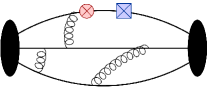
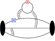
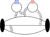
Figure 1: Illustration of one of the connected quark line diagram contributing to the qcEDM (left), the one loop disconnected diagram (middle) and the two loop disconnected diagram (right). The circle indicates the insertion of the electromagnetic current, and the square the qcEDM operator.

III Method for calculating the Matrix Elements of the qcEDM operator

$$\vbox{\hbox{\includegraphics[width=65.04034pt]{qEDM}}}\times{}$$

$$\left(\;\vbox{\hbox{\includegraphics[width=173.44534pt]{cEDM_3pt_disc}}}+\vbox{\hbox{\includegraphics[width=173.44534pt]{cEDM_3pt_orig}}}\;\right)$$

Figure 2: The full calculation requires the reweighting factor times the sum of the connected and disconnected diagrams.

ID	$a$ (fm)	$M_{\pi}$ (MeV)	$L^{3}\times T$	$N_{conf}$
$a12m310$	$0.1207(11)$	$310.2(2.8)$	$24^{3}\times 64$	1013
$a12m220L$	$0.1189(09)$	$227.6(1.7)$	$40^{3}\times 64$	475
$a09m310$	$0.0888(08)$	$313.0(2.8)$	$32^{3}\times 96$	447
$a06m310$	$0.0582(04)$	$319.3(0.5)$	$48^{3}\times 144$	72

Table 1: MILC HISQ ensembles and the simulation parameters used in the analysis. For each lattice configuration, the observables are measured on 128 source positions.

The calculations presented here use the nonunitary clover-on-HISQ formulation, in which correlation functions are calculated using Wilson-clover fermions on four ensembles of background gauge configurations generated with $2+1+1$-flavors highly improved staggered quarks (HISQ) by the MILC collaboration [55]. The lattice parameters are specified in Table 1 and the gauge fields are smoothed using HYP-smearing [56] before calculating the correlation functions. Three of these ensembles, $a12m310$, $a09m310$, and $a06m310$, have a pion mass of $M_{\pi}\approx 315\rm~{}MeV$ and three different lattice spacings, $a\approx 0.12$, $0.09$, and $0.06\rm~{}fm$, respectively, to study the continuum limit. The fourth ensemble, $a12m220L$, at $a\approx 0.12\rm~{}fm$, $M_{\pi}\approx 225\rm~{}MeV$ provides a first check on the dependence on $M_{\pi}^{2}$. For the valence quarks, the clover coefficient was fixed at its tadpole-improved value $c_{sw}=1/u_{0}^{3}$, where $u_{0}$ is the fourth root of the plaquette on the smoothed lattices. Further details of the ensembles, the quark mass parameters, methodology, statistics, and the interpolating operator used in the construction of two- and three-point correlators are given in our previous publications [57, 58, 59, 44].

Working within the framework of the Schwinger source method to calculate the contribution of qcEDM to the nEDM [52] allows us to recast the challenging calculation of the 4-point function given in Eq. 3 and depicted in Fig. 1 to a still difficult but well-exercised calculation of three-point functions [52]. The quark-level diagrams needed to calculate $\langle N|J_{\mu}^{\rm EM}(q)|N\rangle$ in the presence of qcEDM interactions are illustrated in Fig. 2. The steps in each measurement are as follows:

• Calculate propagators, labeled $P$ in Fig. 2, using the standard Wilson-clover Dirac operator, which in the continuum EFT notation reads

  $$O_{D} =D_{L}+m_{W}$$

  $$D_{L} =\not{D}-a\,\left(\frac{r}{2}D^{2}+\kappa_{SW}\sigma\cdot G\right)$$

  $$\qquad\kappa_{SW} =\frac{r}{4}\,c_{SW}~{},$$ (15)

  with $m_{W}\equiv\frac{1}{2\kappa}-4$ the Wilson mass and $c_{SW}=1+O(g^{2})$ the Sheikholeslami-Wohlert coefficient. This calculation of $P$ uses the same methodology as in our previous publications [58]. We assume isospin symmetry so the propagators for $u$ and $d$ quarks are numerically the same.

• Calculate a second set of propagators that include the qcEDM term with coefficient $\epsilon_{q}\equiv-(2\tilde{d}_{q})/(ar)$. This is done by modifying the clover term in the Dirac matrix:

  $$\qquad\frac{rac_{SW}}{4}\sigma^{\mu\nu}G_{\mu\nu} \mathbin{{\longrightarrow}}$$

  $$\frac{ra}{4}\sigma^{\mu\nu}(c_{SW}+i\epsilon_{q}\gamma_{5})G_{\mu\nu}\,.$$ (16)

  We have allowed the qcEDM operator insertion to have different coefficients for the two flavors to make explicit what would need to be done to study the flavor diagonal qcEDM insertions in future work. Choosing $\epsilon_{u}=-\epsilon_{d}=\epsilon$ corresponds to inserting the isovector qcEDM operator $C^{(3)}$ with coefficient $\tilde{d}=-(ar\epsilon)/2$, see Eq. 7. These propagators, labeled $P_{\epsilon}$, include the full effect of inserting the qcEDM operator at all possible intermediate points. Naively, the cost of this inversion is larger by about $7\%$ with respect to $P$, however, using $P$ as the starting guess in the inversion for $P_{\epsilon}$ reduces the number of iterations by 20–40% depending on the quark mass. Overall, the average cost of calculating $P_{\epsilon}$ is about 80% of $P$.

• As discussed below, in order to remove power divergences from isovector qcEDM operator, we need to also calculate insertions of the isovector pseudoscalar density operator $P^{(3)}=i\bar{\psi}\gamma_{5}T^{3}\psi$. We implement this with the replacement

  $$am_{W}\to am_{W}-2i\epsilon_{5}\gamma_{5}\ T_{3}$$ (17)

  in the up and down quark propagators. This prescription corresponds to inserting the operator $P^{(3)}$ with coefficient given by $(-2\epsilon_{5}/a)$.

• Using $P$ and $P_{\epsilon}$, we construct four kinds of sequential sources, labeled $P_{u}^{\rm seq}$, $P_{d}^{\rm seq}$, $P_{-\epsilon,u}^{\rm seq}$, and $P_{-\epsilon,d}^{\rm seq}$. These sources are at the sink time-slice and include the insertion of a neutron at zero momentum and the spin projection operator $(1+\gamma_{4})(1+i\gamma_{5}\gamma_{3})/2$. The subscripts $u$ or $d$ in $P_{u}^{\rm seq}$ and $P_{d}^{\rm seq}$, and similarly in $P_{-\epsilon,u}^{\rm seq}$ and $P_{-\epsilon,d}^{\rm seq}$, denote the flavor of the free spinor in this neutron source. For the backward moving sequential propagators with qcEDM insertion, the coupling gets a minus sign, i.e., $-\epsilon$.

• In our implementation, a number of calculations are done in the same computer job by placing independent sources with maximal separation in time. The corresponding sequential sources are added together to obtain the coherent sequential source [60, 57], which is then used in the construction of the four types of sequential propagators listed above and illustrated in the four correlation functions shown in the right half of Fig. 2.

• The connected three-point function is then calculated using the two original and the four sequential propagators, and with the insertion of $J_{\mu}^{\rm EM}$ separately on the $u$ and $d$ quark lines. This construction is similar to those used in our study of the CP-conserving form-factors [57, 58, 59]. The difference here is the combinations involve propagators with and without the insertion of $\cancel{\text{CP}}$ term as shown in the four three-point functions in the right half of Fig. 2.

• Looking to the future, to construct the disconnected quark loop contribution, the electromagnetic current would be inserted in the quark loop, with and without the qcEDM term, and correlated with the appropriate nucleon two-point correlation functions as illustrated in the left half of Fig. 2. The loop term is integrated over the time-slice $t$ and should be calculated for each of the quark flavors, $u,\ d,\,s,\ c$ and $b$. In this first study, neglect these disconnected diagrams since they are expensive to simulate and their effect is expected to be small.

• We correct for not having included the qcEDM operator in the action in the generation of the gauge configurations by re-weighting the configurations by the ratio of the determinants of the Dirac operators for the two theories:

  $$\frac{\det(\not{D}+m_{W}-\frac{ra}{2}D^{2}-\frac{ra}{4}\sigma^{\mu\nu}(c_{SW}+i\epsilon_{q}\gamma_{5})G_{\mu\nu}))}{\det(\not{D}+m_{W}-\frac{r}{2}aD^{2}-\frac{rc_{SW}}{4}\sigma^{\mu\nu}aG_{\mu\nu})}$$

  $$=\exp\mathop{\rm Tr}\nolimits\ln\left[1-i\epsilon_{q}\frac{ra}{4}\,{\sigma^{\mu\nu}\gamma_{5}G_{\mu\nu}}\left(\not{D}+m_{W}-\frac{r}{2}aD^{2}-\frac{rc_{SW}}{4}\sigma^{\mu\nu}aG_{\mu\nu}\right)^{-1}\right]$$

  $$=\exp\left[-i{\epsilon_{q}}\frac{ra}{4}\mathop{\rm Tr}\nolimits{\sigma^{\mu\nu}\gamma_{5}G_{\mu\nu}}\left(\not{D}+m_{W}-\frac{r}{2}aD^{2}-\frac{rc_{SW}}{4}\sigma^{\mu\nu}aG_{\mu\nu}\right)^{-1}\right]+O(\epsilon^{2})\,.$$ (18)

  The trace in the exponential cancels between the up and down quark contributions when the inserted chromo-EDM is isovector, i.e., $\epsilon_{u}=-\epsilon_{d}=\epsilon$. In general, this factor, the volume integral of the quark loop with the qcEDM insertion, has to be calculated for each active flavor. To implement re-weighting, the sum of the connected and disconnected contributions has to be multiplied by the exponential of the sum of the qcEDM loop with the appropriate coupling $i\epsilon_{q}$ for each flavor. This is shown by the overall factor in Fig. 2. In short, for the isovector qcEDM operator analyzed here, all disconnected contributions are either neglected or cancel.

  Ensemble	qcEDM		$\gamma_{5}$
  	$\epsilon$	$\alpha/\epsilon$	$\epsilon_{5}$	$\alpha_{5}/4\epsilon_{5}$
  a12m310	0.0080	$-$10.835(55)	0.0024	$-$8.908(45)
  a12m220L	0.0010	$-$21.80(31)	0.0003	$-$17.88(24)
  a09m310	0.0080	$-$12.360(36)	0.0024	$-$12.052(34)
  a06m310	0.0080	$-$15.00(12)	0.0012	$-$19.82(16)

  Table 2: The couplings $\epsilon$ and $\epsilon_{5}$ used in the simulations with the qcEDM and pseudoscalar operators, and the corresponding neutron phases, $\alpha$ and $\alpha_{5}$, obtained on each ensemble from fits shown in Fig. 3.

• The above calculation is repeated for different values of $\epsilon$ to extract $F_{3}(0)$ as a function of $\epsilon$. The contribution to the neutron electric dipole moment of the qcEDM operator is then given by the slope versus $\epsilon$. In the dimensionless parameter $X_{c}$ defined in Eq. 9, taking the limit is not required for sufficiently small $\epsilon$, which is in the linear regime.

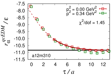
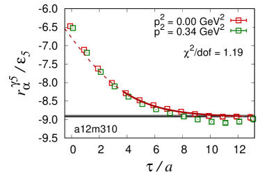
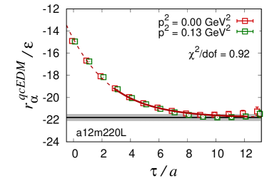
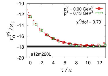
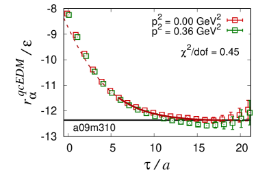
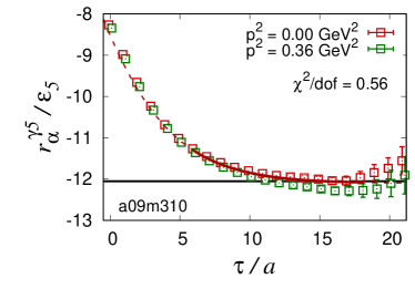
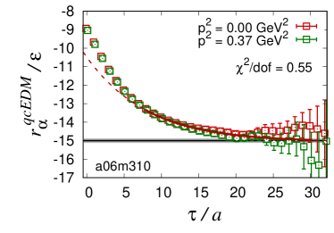
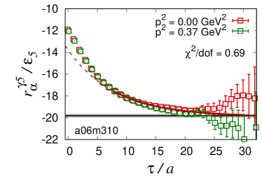
Figure 3: A 2-state fit to the ratio $r_{\alpha}$ defined in Eq. 19 used to extract the isovector CP violating phase $\alpha$ for the insertion of the qcEDM (left) and pseudoscalar (right) operators. The phase is independent of the momentum of the state and the results are summarized in Table 2.

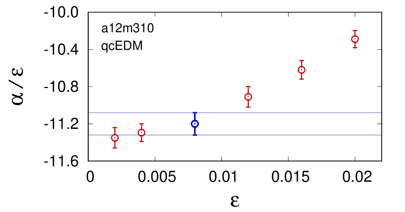
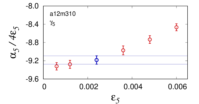
Figure 4: The value of the phase $\alpha$ ($\alpha_{5}$) as a function of the qcEDM (pseudoscalar) coupling $\epsilon$ ($\epsilon_{5}$). For small enough $\epsilon$, the $\mathcal{O}(\epsilon^{2})$ contributions become negligible and $\alpha/\epsilon$ should be a constant for different choices of $\epsilon$. The blue data points within the linear region show the $\epsilon$ used in the main simulation. The data shown are obtained using 50 configurations of the a12m310 ensemble.

III.1 The extraction of the $\cancel{\text{CP}}$ phase $\alpha_{N}$

The first step in the calculation is to extract the $\cancel{\text{CP}}$ phase $\alpha_{N}$, defined through Eq. 10, from the nucleon two-point functions. Since this phase is state-dependent, its value for the ground state nucleon has to be extracted at large source-sink separations where ESC have died out as described in our previous work [44]. The data and the fits for the four ensembles and with the insertion of $\epsilon$ and $\epsilon_{5}$ are shown in Fig. 3 and the results summarized in Table 2. The behavior of $\alpha_{N}$ versus $\epsilon$ is shown in Fig. 4, which we use to select the value of $\epsilon$ that is small enough to lie in the linear regime and yet large enough to give a good statistical signal. This value is highlighted in Figs. 3 and 2.

To extract the phase, we calculate the ratio [44]

$$r_{\alpha}(\tau) \equiv\frac{\Im\mathop{\rm Tr}\nolimits\gamma_{5}\frac{1+\gamma_{4}}{2}\langle N(0)\overline{N}(\tau)\rangle}{\Re\mathop{\rm Tr}\nolimits\frac{1+\gamma_{4}}{2}\langle N(0)\overline{N}(\tau)\rangle}$$

$$\approx\tan\alpha_{0}\times\frac{1+\frac{\sin(2\alpha_{1})}{\sin(2\alpha_{0})}|\tilde{\cal A}_{1}|^{2}\ e^{-(M_{1}-M_{0})\tau}}{1+\frac{\cos^{2}(\alpha_{1})}{\cos^{2}(\alpha_{0})}|\tilde{\cal A}_{1}|^{2}\ e^{-(M_{1}-M_{0})\tau}}\,,$$ (19)

which approaches $\alpha_{N}\equiv\alpha_{0}$ at large $\tau$ and allows us to extract $\alpha_{N}$ from a fit [44].

IV Pseudoscalar density versus quark chromo-EDM insertions

In this section we discuss the connection between insertions of the isovector qcEDM operator and the isovector pseudoscalar density at finite lattice spacing $a$. The discussion is based on the framework of a continuum EFT for the lattice action and the axial Ward Identities, following Refs. [61, 62]. We first discuss the nonsinglet axial Ward identity and the relation between chromo-EDM and pseudoscalar density that follows from it. We then present the lattice analysis to determine the relevant nonperturbative coefficients arising in the mixing.

IV.1 Nonsinglet axial Ward identity and implications

We will denote by $O_{n}^{(d)}$, $\tilde{O}_{n}^{(d)}$, $O_{n}^{(d),{\rm ren}}$, the set of bare, subtracted, and renormalized operators of dimension $d$, respectively. Subtracted operators, i.e. operators free of power divergences, are defined as

$$\tilde{O}_{n^{\prime}}^{(d)}=O_{n^{\prime}}^{(d)}-\sum_{d^{\prime}<d,k}\frac{\beta_{n^{\prime}k}^{(d)}}{a^{d-d^{\prime}}}\,\tilde{O}_{k}^{(d^{\prime})}$$ (20)

with the sum over $k$ running over all operators of dimension $d^{\prime}$. The finite (renormalized) operators are given by

$$O_{n}^{(d),{\rm ren}}=Z_{nn^{\prime}}\ \tilde{O}_{n^{\prime}}^{(d)}~{}.$$ (21)

The presence of $\tilde{O}_{k}^{(d^{\prime})}$ and not $O_{k}^{(d^{\prime})}$ in Eq. 20 is needed to avoid ambiguities in the definition of coefficients $\beta_{n^{\prime}k}^{(d)}$ of lower-dimensional operators.

As derived in Appendix A, under the axial transformation on the quark fields collectively defined by $\psi^{T}=(u,d,s,c)$

$$\psi(x) \to(1+i\xi^{(a)}(x)T^{a}\gamma_{5})\psi(x)$$

$$\bar{\psi}(x) \to\bar{\psi}(x)(1+i\xi^{(a)}(x)T^{a}\gamma_{5})\,,$$ (22)

where $\xi^{(a)}(x)$ is the local chiral transformation parameter and $T^{a}$ are the generators of flavor $SU(4)$, the flavor nonsinglet axial Ward Identity (AWI) for the expectation value of $O$ is given by

$$\int d^{4}x\Big{\langle}O(x_{1},...,x_{n})\times{}\hskip 99.73074pt$$

$$\Big{[}-\bar{\psi}(x)\{m,T^{a}\}\gamma_{5}\psi(x)\Big{(}1+O(am)\Big{)}-$$

$$\qquad\qquad\qquad aiK_{X1}\ \tilde{C}^{(a)}\Big{]}\Big{\rangle}$$

$$=-\int d^{4}x\left\langle\frac{\delta O(x_{1},...,x_{n})}{\delta(i\xi^{(a)}(x))}\right\rangle\,.$$ (23)

This is correct up to $O(a^{2})$ corrections when applied to the Wilson-clover fermion action that includes $O(a)$ hard breaking of chiral symmetry. Here, $K_{X1}$ is a nonperturbative constant that characterizes the $O(a)$ breaking of chiral symmetry, and vanishes if the theory is fully $O(a)$ improved. The RHS of Eq. 23 does not contribute to on-shell matrix elements, and hence to the form factor $F_{3}$. In this case, insertions of the iso-vector pseudoscalar density are proportional to insertions of the subtracted iso-vector quark chromo-EDM operator. In the next subsection, we show how an analysis of the unintegrated version of this equation given in Eq. 46 allows us to determine the needed nonperturbative factor $K_{X1}$ relating the two operators.

IV.2 Determining the nonperturbative parameters

We now specialize to the isovector case, corresponding to the flavor index $a=3$. We also work in the isospin limit and denote the common light quark masses by $m_{l}$. Taking the pion field to be $P^{(3)}\equiv i\overline{\psi}\gamma_{5}T^{3}\psi$, and specializing to $O(x_{1},...,x_{n})\to O(z)$, Eq. 46 becomes

$$\Big{\langle}O(z)\Big{[}Z_{A}\,(1+b_{A}m_{l}a)\,\partial_{\mu}A_{\mu}^{(3)}(x)+{}$$

$$iaZ_{A}c_{A}\,\partial^{2}P^{(3)}(x)+2m_{l}iP^{(3)}(x)-{}$$

$$\qquad\qquad aiK_{X1}\ \tilde{C}^{(3)}(x)\Big{]}\Big{\rangle}$$

$$=-\Big{\langle}\frac{\delta O(z)}{\delta(i\xi^{3}(z))}\Big{\rangle}\,,$$ (24)

up to $O(a^{2})$ corrections. In order to determine $K_{X1}$, we need to first define $\tilde{C}^{(3)}$.

Ensemble	$c_{SW}$	$a$ (fm)	$t$-range	$A$
a12m310	1.05094	0.1207(11)	6–14	$1.21374(62)$
a12m220L	1.05091	0.1189(09)	7–14	$1.21800(33)$
a09m310	1.04243	0.0888(08)	8–22	$0.99621(30)$
a06m310	1.03493	0.0582(04)	14–30	$0.77917(24)$

Table 3: Determination of $A$ defined in Eq. 25 from an average over the plateau region ($t$-range) of ratios of two-point functions.

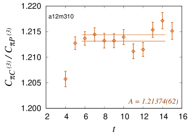
Figure 5: Data from a12m310 ensemble showing the determination of the subtraction coefficient $A$ using Eq. 26 (upper panel), and the coefficients $\bar{c}_{A}$, $\bar{K}_{X1}$ and $2\bar{m}a$ using Eq. 29 (lower panel).

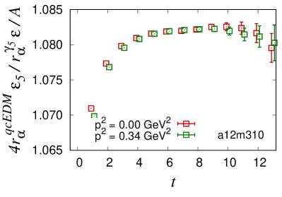
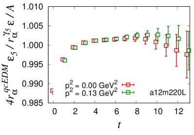
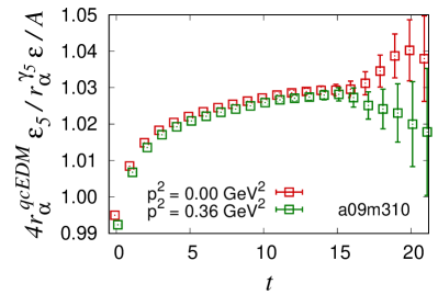
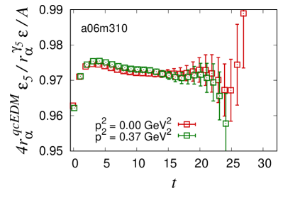
Figure 6: Test of the relation given in Eq. (27). The ratios $r_{\alpha}$, defined in Eq. (19), give the CP violating phases $\alpha_{N}$. The mixing coefficient $A$ is defined in Eq. (25).

IV.2.1 Determination of parameter $A$

As explained in Appendix B, under isospin symmetry and when applied to on-shell zero momentum correlators, Eq. 20, which relates the subtracted qcEDM operator to the bare un-subtracted one used in the lattice calculation, reduces to

$$\tilde{C}^{(3)}(x)=C^{(3)}(x)-\frac{A}{a^{2}}P^{(3)}(x)~{},$$ (25)

where $A$ is $O(\alpha_{s})$ with $O(am)$ and convention-dependent $O(a^{2})$ corrections. To determine $A$, we can, for example, define $\tilde{C}^{(3)}$ by demanding $\langle\Omega|\tilde{C}^{(3)}|\pi(\vec{p}=0)\rangle=0$. This is particularly simple to implement on the lattice—we, in the two-point functions $C_{\pi P^{(3)}}(t)=\langle TP^{(3)}(t)\pi(0)\rangle$ and $C_{\pi C^{(3)}}(t)=\langle TC^{(3)}(t)\pi(0)\rangle$, place the pseudoscalar and qcEDM interpolating operators at the sink and use the same pion source, $\pi(0)$. Since the pion ground state dominates these two-point functions at long distances, the coefficient $A$ is given by the asymptotic behavior of their ratio:

$$A=\lim_{t\to\infty}\frac{a^{2}C_{\pi C^{(3)}}(t)}{C_{\pi P^{(3)}}(t)}\,.$$ (26)

Other choices of correlation functions used to determine $A$ change only the convention-dependent $O(a^{2})$ contributions. As shown in Tables 3 and 5, this construction gives a very precise determination of $A$. Though formally $O(\alpha_{s})$, its value is close to unity at values of the lattice spacing where current simulations have been done.

We can use this determination of $A$ to perform a consistency check on the phases $\alpha_{N}^{5}$ and $\alpha_{N}$ induced by the $\cancel{\text{CP}}$ operators $P^{(3)}$ and $C^{(3)}$, respectively. As described in Appendix D, at leading order in chiral perturbation theory ($\chi$PT), $\tilde{C}^{(3)}$ defined in Eq. 25 gives no contribution to $\alpha_{N}$. Then, from the right hand side we expect the relation (see Eq. 62).

$$\frac{1}{A}\frac{\alpha_{N}}{\alpha_{N}^{5}}=1+O\left(\frac{m_{\pi}^{2}}{\Lambda_{\chi}^{2}}\right)\,.$$ (27)

Since $\alpha$ is state dependent, the determination of $\alpha_{N}$ ($\alpha_{N}^{5}$) are straightforward only when extracted at asymptotically long Euclidean times where ESC are negligible. Since the signal-to-noise in nucleon correlators degrades exponentially, this asymptotic region cannot be reached with current statistics. Instead, we analyze $r_{\alpha}$ defined in Eq. 19 that includes the lowest excited state contributions. Data in Fig. 6 for the four ensembles show that the relation Eq. 27 is satisfied to within ten percent by the $\alpha$ we determine.

IV.2.2 Determination of parameter $K_{X1}$

In terms of the unsubtracted $C^{(3)}$, the nonsinglet AWI, Eq. 24, can now be cast as follows:

$$\Big{\langle}O(z)\Big{[}Z_{A}\,(1+b_{A}ma)\,\partial_{\mu}A_{\mu}^{(3)}(x)+{}$$

$$iaZ_{A}c_{A}\,\partial^{2}P^{(3)}(x)+i{2m}P^{(3)}(x)$$

$${}-i{K_{X1}}\left(a\ C^{(3)}(x){-\frac{A}{a}P^{(3)}}\right)\Big{]}\Big{\rangle}$$

$$=-\Big{\langle}\frac{\delta O(z)}{\delta(i\xi^{(3)}(x))}\Big{\rangle}\,.$$ (28)

To calculate $K_{X1}$ and $m$, consider the two point functions $C_{\pi A_{\mu}^{(3)}}(t)$, $C_{\pi P^{(3)}}(t)$ and $C_{\pi C^{(3)}}(t)$ of $A_{4}^{(3)}(t)$, $P^{(3)}(t)$ and $aC^{(3)}(t)$ with a common source $\pi(0)$. Further, let $\Delta$ and $\Delta^{2}$ define the symmetric lattice first and second derivatives in the time direction: e.g., $(\Delta C)(t)\equiv[C(t+1)-C(t-1)]/2$ and $(\Delta^{2}C)(t)\equiv[C(t+1)+C(t-1)-2C(t)]$. Then, on-shell, i.e., at $t\not=0$, we have

$$\frac{ia\Delta C_{\pi A_{4}^{(3)}}(t)-\bar{c}_{A}a^{2}\Delta^{2}C_{\pi P^{(3)}}(t)+{\bar{K}_{X1}}\left(a^{2}C_{\pi C^{(3)}}(t){-AC_{\pi P^{(3)}}(t)}\right)}{C_{\pi P^{(3)}}(t)}={2\bar{m}a}\ +\ O(a^{2}m^{2},a^{2}\Lambda_{QCD}^{2})~{},$$ (29)

where

$$\bar{c}_{A} =\frac{c_{A}}{(1+b_{A}ma)}$$ (30a)

$${\bar{K}_{X1}} =\frac{{K_{X1}}}{Z_{A}(1+b_{A}ma)}$$ (30b)

$${\bar{m}} =\frac{{m}}{Z_{A}(1+b_{A}ma)}\,.$$ (30c)

Thus, one can extract the coefficients $\bar{c}_{A}$ and ${\bar{K}_{X1}}$ by fitting the left hand side and requiring it be independent of $t$ and the pion interpolating field $\pi$. Simultaneously, the fit provides ${2\bar{m}a}$, and thus ${K_{X1}}/{2ma}$, which is required next.

We implemented the identity Eq. 29 numerically by choosing $\pi$ to be the pseudoscalar interpolating operator $P^{(3)}$ constructed using Wuppertal-smeared sources for quark propagators with various radii and at various momentum. As discussed in Appendix C, these three-parameter fits are very unstable with our statistics. We, therefore, proceeded by noting that the factor multiplying $\bar{K}_{X1}$ vanishes once the contribution of the excited states vanish. Thus, we first make a two-parameter fit to the large-$t$ region ignoring $\bar{K}_{X1}$. We then hold $c_{A}$ fixed and determine $\bar{K}_{X1}$ by extending the region to smaller $t$. The results are given in Table 4.

	fit-range		$\chi^{2}/\rm d.o.f$
Ensemble	$c_{A}$	${\bar{K}}_{X1}$	$c_{A}$	${\bar{K}}_{X1}$	$c_{A}$	${\bar{K}_{X1}}$	${2\bar{m}a}$	$\displaystyle\frac{2ma}{K_{X1}}$	$\displaystyle\frac{2ma}{2ma+AK_{X1}}$
a12m310	4–11	3–11	0.66	0.88	$0.054(10)$	$0.097(45)$	$0.02205(46)$	$0.23(10)$	$0.158(58)$
a12m220L	4–11	3–11	2.08	3.09	$0.0342(77)$	$0.183(35)$	$0.01152(21)$	$0.063(12)$	$0.0491(86)$
a09m310	5–15	4–15	0.99	1.09	$0.0277(40)$	$0.047(15)$	$0.01684(15)$	$0.35(11)$	$0.263(61)$
a06m310	6–20	5–20	0.29	1.53	$0.0093(17)$	$0.0272(60)$	$0.010460(37)$	$0.385(87)$	$0.331(50)$

Table 4: The determination of ${\bar{K}}_{X1}$ and $2{\bar{m}}a$, and their ratios $2ma/K_{X1}$ and $2ma/(2ma+AK_{X1})$ using Eq. (29) and see the discussion below it.

IV.3 Implications for the nEDM

The relation Eq. 23 implies that, up to $O(a^{2})$ effects, insertions of the subtracted isovector qcEDM and the pseudoscalar operators at zero four-momentum transfer and between on-shell states are proportional to each other. Furthermore, Eq. 28, for zero-momentum on-shell matrix elements, gives $\langle P^{(3)}\rangle={[K_{X1}/(2ma+AK_{X1})]}\langle a^{2}C^{(3)}\rangle$, a relation between unsubtracted operators. Thus, we have the following relations between subtracted and unsubtracted isovector operators up to $O(a^{2})$:

$$a\tilde{C}^{(3)} ={\frac{2am}{K_{X1}}}\frac{P^{(3)}}{a}$$ (31a)

$$a\tilde{C}^{(3)} =\left({\frac{2am}{2am+AK_{X1}}}\right)aC^{(3)}\,.$$ (31b)

Note that even though both the quantities $K_{X1}\sim O(\alpha_{s})$ and $2am$ are small, for values of the lattice spacing $a$ used in current simulations, their ratio is $O(1)$. In the continuum limit, $P^{(3)}$ can be rotated away, but Eq. 31a shows that at $a\sim 0.1\rm fm$, the effect of the lattice operators $P^{(3)}/a$ and $aC^{(3)}$ are comparable.

Furthermore, if $c_{SW}$ is nonperturbatively tuned, there are no $O(a)$ effects and $K_{X1}$ vanishes, $P^{(3)}$ gives no contributions and $\tilde{C}^{(3)}=C^{(3)}$ to this order. Finally, we remark that, in the continuum limit $a\to 0$, chiral symmetry is broken only by the qcEDM term as $m\to 0$, therefore, its entire effect can be rotated away, i.e., $\tilde{C}^{(3)}$ gives no contribution to physics in these limits [49]. At finite $a$, the same holds true at $O(a)$.

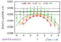
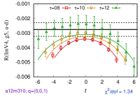
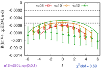
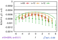
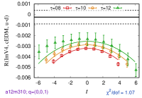
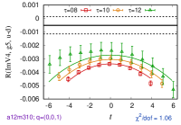
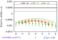
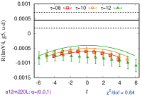
Figure 7: Fits to remove ESC and obtain ground state matrix elements from correlation functions with the insertion of $\rm qcEDM$ and $\gamma_{5}$ operators along with the $V_{4}$ current at momentum transfer $q=(0,0,1)$. Data are shown for the a12m310 and a12m220L ensembles. (Top) “Standard” excited state fit with the mass gaps taken from fits to the two-point function. (Bottom) “$N\pi$” excited state fits assuming the first excited state is $N(0,0,1)\pi(0,0,0)$, i.e., the energy gap is $M_{\pi}$. The form factor ${\widetilde{F}}_{3}$ is extracted from such matrix elements.

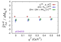
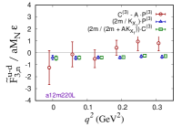
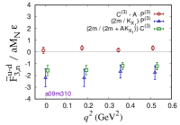
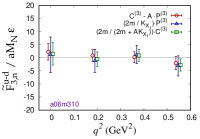
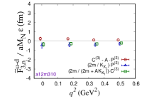
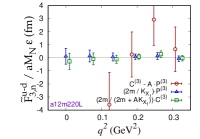
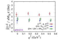
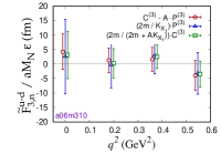
Figure 8: The form factor ${\tilde{F}}_{3,n}^{u-d}/aM_{N}\varepsilon$ using the subtracted qcEDM operator for the three different subtraction approaches specified in the labels and given in Eqs. 25, 31a and 31b. Top figures are the results from the four ensembles using the “Standard” excited state fit, and the bottom figures are the result of using the “$N\pi$” excited state fits as explained in the text. Differences between the three approaches specified by the labels are due to residual $O(a)$ artifacts in our action, which vanish in the continuum limit. As explained in the text, we consider estimates using $C^{(3)}-AP^{(3)}$ (red circles) are the least reliable.

V Exploratory numerical calculations

Ensemble	${\tilde{F}}_{3}^{\gamma_{5}}/{\tilde{F}}_{3}^{\rm qcEDM}$					$\displaystyle\frac{K_{X1}}{2am+AK_{X1}}$
	$Q^{2}=1$	$Q^{2}=2$	$Q^{2}=3$	$Q^{2}=4$	$Q^{2}=5$
a12m310	0.879(17)	0.863(14)	0.867(18)	0.844(23)	0.864(13)	0.694(48)
a12m220L	0.81(10)	0.769(77)	0.869(75)	0.98(18)	0.94(11)	0.7807(70)
a09m310	1.063(35)	1.042(40)	1.078(45)	1.006(58)	1.039(44)	0.740(61)
a06m310						0.859(64)

Table 5: The ratio ${\tilde{F}}_{3}^{\gamma_{5}}/{\tilde{F}}_{3}^{\rm qcEDM}$ for the $\gamma_{5}$ and $\rm qcEDM$ unsubtracted lattice operators for the five smallest values of $Q^{2}$. As expected, the ratios are, within errors, independent of $Q^{2}$ and the quark mass, and close to the $K_{X1}/(2am+AK_{X1})$ obtained from the pion correlators (last column) using Eq. (29). We do not find a significant signal in ${\tilde{F}}_{3}^{\gamma_{5}}/{\tilde{F}}_{3}^{\rm qcEDM}$ with the current data for the $a06m310$. The data for ${\tilde{F}}_{3}$ are obtained using the “standard” method for removing excited state contamination.

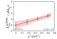
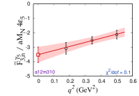
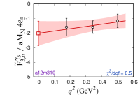
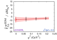
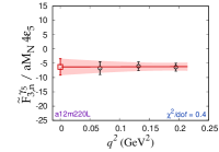
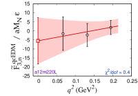
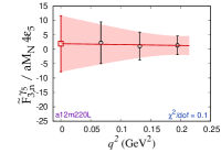
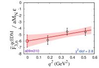
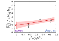
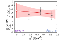
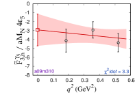
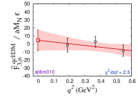
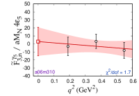
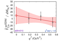
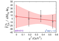
Figure 9: Dependence of ${\tilde{F}}_{3}$ on $Q^{2}$ for the neutron obtained from the insertion of the qcEDM and $\gamma_{5}$ operators. Data in the left two columns are obtained using the “Standard” fit to control ESC, and in the right two columns, using the “$N\pi$”. The latter have much larger errors.

We use the method previously described in Ref. [44] for calculating the contribution of $\cancel{\text{CP}}$ interactions that are based on extracting the form-factor $F_{3}$. In this method, it is essential to remove the ESC in going from 3-point functions to matrix elements as discussed for the $\cancel{\text{CP}}$ $\Theta$-term in Ref. [44]. The methods we use are described in [63, 64, 65, 44].

We also caution the reader that, here on, all the data for the $\cancel{\text{CP}}$ form factor $F_{3}$ will be presented in terms of ${\tilde{F}}_{3}$ defined in [44]. It can be extracted more reliably on the lattice and ${\tilde{F}}_{3}(0)=F_{3}(0)$ in the limit of interest, $Q^{2}=0$.

In Fig. 7, we show examples of fits used to remove ESC in correlation functions with the insertion of $V_{4}$ in the presence of the qcEDM and $\gamma_{5}$ operators from which ${\tilde{F}}_{3}$ is extracted. In these fits, we consider two possible values for the first excited-state energy as discussed in Ref. [44] for the similar case of the $\Theta$-term: (i) the “standard” fit with the energy given by the two-point function, and (ii) the “$N\pi$” fit using the non-interacting energy of the $N\pi$ state. While the results depend sensitively on the excited state spectrum used in the analysis, the fits have similar $\chi^{2}/dof$, i.e., the fits do not provide an objective selection criteria. The data in Fig. 8 and the final results in Section VI highlight the size of this uncontrolled systematic, which needs to be addressed in future calculations.

We now discuss the calculation of the parameter $K_{X1}$, which arises if there is residual $O(a)$ chiral symmetry breaking, and the extraction of ${\tilde{F}}_{3}$. The data are from the “standard” method for removing excited state contamination.

From Eqs. 31a and 31b, we note that the ratio ${\tilde{F}}_{3}(P^{(3)})/F_{3}(C^{(3)})=K_{X1}/(2am+AK_{X1})+O(a^{2})$. We, however, notice that the $O(a^{2})$ terms are likely to be large; in fact, the $O(a^{2}\Lambda_{\rm QCD}^{2})\sim 0.01\hbox{--}0.04$ corrections on the right hand side of Eq. 29 may provide a substantial correction to the leading term, $O(2am)\sim 0.01$. We study this by noting that under the assumption that corrections are small, all numbers in a given row of Table 5 should agree. This is roughly true for the different $Q^{2}$, but the $O(25\%)$ difference between ${\tilde{F}}_{3}^{\gamma_{5}}/{\tilde{F}}_{3}^{\rm qcEDM}$ and $K_{X1}/(2am+AK_{X1})$, is indicative of $O(a^{2})$ effects. A similar effect is anticipated in $\tilde{F}_{3}(Q^{2})$ calculated using the three subtraction schemes defined in Section IV, and shown in Fig. 8. The determinations using Eqs. 31a and 31b are close, however, they could both have large $O(a^{2})$ effects coming from the Ward identity. The direct determination, Eq. 25, can also have large $O(a^{2})$ effects and is a difference of two numbers of similar size. Furthermore, any difference between estimates using Eqs. 31a and 31b will get magnified by the large factor $AK_{X1}/2am$, to give a large difference from the direct determination, Eq. 25, value. In short, at this stage, we do not have control over $O(a^{2})$ errors. Looking at Fig. 8, estimates from the direct determination have large fluctuations on the $a12m220L$ ensemble, are consistent with the other two on $a06m310$, and show a large difference on the remaining two. Estimates from Eqs. 31a and 31b are consistent. Of these, we choose the results from Eq. 31b in our final analyses because they have lower statistical errors.

The extraction of ${\tilde{F}}_{3}$ at $Q^{2}=0$ is carried out using an extrapolation linear in $Q^{2}$ using data at the three smallest values of $Q^{2}$ as shown in Figure 9. To estimate the systematic uncertainty due to choosing the linear ansatz, we use the difference between the extrapolated $\tilde{F}_{3}(0)$ and the $\tilde{F}_{3}(Q^{2})$ at the smallest nonzero $Q^{2}$.

Ensemble	qEDM		$X_{c}$, Standard Fit		$X_{c}$, $N\pi$ Fit
	$g_{T}^{u}$	$g_{T}^{d}$	Lattice	2 GeV	Lattice	2 GeV
a12m310	$0.859(12)$	$-0.206(7)$	$\hphantom{-}0.239(86)$	$\hphantom{-}0.205(85)$	$\hphantom{-}0.28(16)$	$\hphantom{-}0.25(16)$
a12m220L	$0.846(11)$	$-0.203(5)$	$-1.2(1.4)$	$-1.3(1.4)$	$-7.8(5.4)$	$-7.8(5.4)$
a09m310	$0.824(7)$	$-0.203(3)$	$\hphantom{-}0.15(28)$	$\hphantom{-}0.17(28)$	$\hphantom{-}0.55(50)$	$\hphantom{-}0.57(50)$
a06m310	$0.784(15)$	$-0.192(8)$	$\hphantom{-}2.3(3.2)$	$\hphantom{-}2.4(3.2)$	$\hphantom{-}4.3(6.1)$	$\hphantom{-}4.4(6.2)$

Table 6: Results for $X_{c}\equiv d_{N}/{\tilde{d}}$, renormalized in the $\overline{\rm MS}$ scheme at $2$ GeV as explained in the text, are given for the two methods used for removing ESC—without (standard fit) and with a $N\pi$ excited state. The results for the matrix elements of the qEDM operator, which are given by the tensor charges, $g_{T}^{u}$ and $g_{T}^{d}$, are quoted from our published work [58].

VI Renormalization and Chiral-continuum extrapolation

The subtracted isovector qcEDM operator $\tilde{C}^{(3)}(a)$ is free of power divergences but still has logarithmic divergences as $a\to 0$. In the calculation of the nEDM, it is implicit that one has to work with $QCD+QED$ since the operator $\tilde{C}^{(3)}$ has to be inserted together with the electromagnetic current in the correlation functions. In this theory, $\tilde{C}^{(3)}$ mixes with the quark EDM operator $E^{(3)}(a)$ defined in Eq. 48c. One therefore, needs to calculate the mixing and running of these two operators. Only the anomalous dimension matrix (universal) part of this has been calculated at $O(\alpha_{s})$ [49]. In this leading-logarithm approximation (tree-level matching and one-loop running), the lattice and $\overline{\rm MS}$ operators are related by

$$\vec{O}_{\overline{\rm MS}}(\mu) =$$

$$\!\!U\begin{pmatrix}\left(\frac{\alpha_{s}(\mu)}{\alpha_{s}(a^{-1})}\right)^{\mathrlap{-\gamma_{11}/\beta_{0}}}&0\\ 0&\left(\frac{\alpha_{s}(\mu)}{\alpha_{s}(a^{-1})}\right)^{-\gamma_{22}/\beta_{0}}\end{pmatrix}U^{-1}\vec{O}(a)$$

where

$$\vec{O}(a) =\begin{pmatrix}\tilde{C}^{(3)}(a)\\ E^{(3)}(a)\end{pmatrix}$$

$$\vec{O}_{\overline{\rm MS}}(\mu) =\begin{pmatrix}C_{\overline{\rm MS}}^{(3)}(\mu)\\ E_{\overline{\rm MS}}^{(3)}(\mu)\end{pmatrix}$$

$$U =\begin{pmatrix}1&-\frac{\gamma_{12}}{\gamma_{11}-\gamma_{22}}\\ 0&1\end{pmatrix}\,,$$ (33)

and

$$\frac{\alpha_{s}(\mu)}{\alpha_{s}(a^{-1})}=\frac{1}{1-\frac{\alpha_{s}(a^{-1})}{\pi}\,\beta_{0}\,\log(\mu a)}~{}.$$ (34)

The coefficients of the $\alpha_{s}/\pi$ term in the beta function and the anomalous dimension matrix are

$$\beta_{0} =\frac{2N_{F}-11N_{C}}{6}\,,$$ (35)

$$\gamma_{11}=\frac{5C_{F}-2C_{A}}{2},\ \gamma_{12}=2C_{F},\ \gamma_{22}=\frac{C_{F}}{2}$$ (36)

with

$$C_{F}=\frac{N_{C}^{2}-1}{N_{C}}~{},\qquad\qquad C_{A}=N_{C}$$ (37)

Using $N_{F}=4$ we obtain

$$-\frac{\gamma_{11}}{\beta_{0}}=\frac{2}{25}~{},\quad-\frac{\gamma_{22}}{\beta_{0}}=\frac{4}{25}~{},\quad U=\left(\begin{array}[]{cc}1&8\\ 0&1\end{array}\right)~{}.$$ (38)

Because the matching is done at tree level and followed by 1-loop running, the renormalization process is insensitive to the scheme. Consequently the data for $X_{c}\equiv-\tilde{F}_{3}(0)/aM_{N}\varepsilon$ (see Eq. 9) carry an unresolved uncertainty of order $\alpha_{s}(\mu)/\pi$. At this order, one can, therefore, choose to use either the renormalized or unrenormalized tensor charges. We have chosen to use the renormaized values given in Ref. [49].

The resulting renormalized values for $X_{c}$ are given in Table 6 for two ways of removing ESC–with and without including an $N\pi$ excited state. Their extrapolation, linear in $a$ and $M_{\pi}$, to the physical point is shown in Fig. 10. The data show no significant dependence on the lattice spacing $a$. The dependence on $M_{\pi}^{2}$ is much larger with the $N\pi$ analysis, however, it is important to note that this chiral behavior is predicated on a single point, i.e., $a12m220L$. The final results in the continuum limit are $X_{c}\equiv-{{F}_{3}(0)/aM_{N}\varepsilon=2.6(2.9)}$ for the “Standard” excited state fit, and ${14(10)}$ for the “$N\pi$” excited state fit, where the quoted errors are statistical.

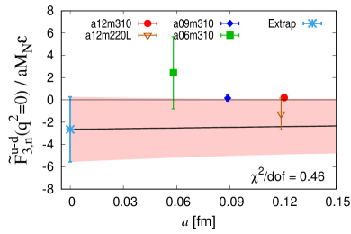
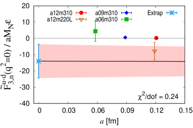
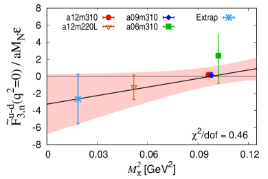
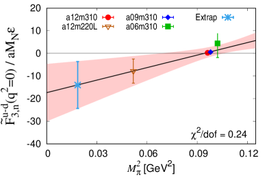
Figure 10: Extrapolation to the continuum and physical pion mass limit using the fit ansatz ${c_{1}+c_{2}M_{\pi}^{2}+c_{3}a}$. Results from different ensembles are renormalized in $\overline{\rm MS}$ scheme at $\mu=2$ GeV using LABEL:eq:renorm. Left column shows the results from the “Standard” excited state fit, and the right column shows the results from the “$N\pi$” excited state fits. Extrapolated values are ${\tilde{F}_{3}(0)/aM_{N}\varepsilon=-2.6(2.9)}$ for the “Standard” excited state fit, and ${\tilde{F}_{3}(0)/aM_{N}\varepsilon=-14(10)}$ for the “$N\pi$” excited state fit.

VII Conclusions

In the analysis of the contribution of the qcEDM operator to nEDM $d_{n}$ presented here, we have focused on the issue of the power-divergent mixing of the qcEDM operator with the quark-pseudoscalar operator. This mixing is independent of the explicit breaking of the chiral symmetry on the lattice, and is generic to all hard cutoff schemes. For the isovector case, the pseudoscalar operator gives no physical effects in the continuum limit; at finite lattice spacing with Wilson-clover fermions, however, it results in an effect proportional to the qcEDM operator itself. This finite lattice spacing artifact is seen in explicit calculations with the isovector pseudoscalar operator, which gives a large EDM signal on the lattice. More importantly, this proportionality turns the divergent mixing into an extra finite multiplicative renormalization of the qcEDM operator, an effect that survives in the continuum limit if the theory is not fully $O(a)$ improved.

We further show that the uncertainty in this finite renormalization constant is substantial if $c_{\rm SW}$ is tuned using tree-level tadpole improvement, i.e., not fully $O(a)$ improved. Any residual, even small, $O(a)$ contribution gets divided by $2am$, an equally small number. We have devised a scheme to determine this finite constant nonperturbatively provided we can ignore $O(a^{2})$ corrections.

Unfortunately, our data show that at close to physical masses and at the values of $a$ used in this study, the $O(a^{2})$ corrections can be as large as $\approx 25\%$. This leads to an irreducible uncertainty in the results, which is in addition to the uncertainty due to the continuum and chiral extrapolations. Using techniques like gradient-flow that remove chiral symmetry breaking, this source of uncertainty can be avoided.

A $\chi$PT analysis presented in Appendix D predicts the ratio of the phase $\alpha$ generated on the insertion of the qcEDM and pseudoscalar operators given in Eq. 27. Our data on the four ensembles (see Fig. 6) show agreement with this analysis within ten percent.

To study excited state contributions in the extraction of ground-state matrix elements of the qcEDM and pseudoscalar operators, we have made fits with two choices of the mass of the first excited state, that from fits to the nucleon 2-point correlation function and the $N\pi$ state. The fits cannot be distinguished by the $\chi^{2}/dof$, however, the results differ by a factor of five.

To obtain a result for the isovector contribution of the qcEDM operator to nEDM, future work needs to address two challenges, in addition to issues of chiral and continuum extrapolation, exposed by this study: (i) possibly large $O(a^{2})$ effects as discussed in Section V and (ii) the difference in estimates between removing ESC with and without including $N\pi$ excited states in the spectral decomposition of the correlation functions as discussed in Section VI.

Acknowledgements: We thank the MILC collaboration for providing the HISQ lattices. The calculations used the CHROMA software suite [Edwards:2004sx]. Simulations were carried out at (i) the NERSC supported by DOE under Contract No. DE-AC02-05CH11231; (ii) the Oak Ridge Leadership Computing Facility, which is a DOE Office of Science User Facility supported under Award No. DE-AC05-00OR22725 through the INCITE program project HEP133, (iii) the USQCD collaboration resources funded by DOE HEP, and (iv) Institutional Computing at Los Alamos National Laboratory. This work was supported by LANL LDRD program. TB, RG and EM were also supported by the DOE HEP and NP under Contract No. DE-AC52-06NA25396. VC acknowledges support by the U.S. DOE under Grant No. DE-FG02-00ER41132.

Appendix A Nonsinglet Axial Ward Identity at $O(a)$

The starting point of the demonstration that, on-shell, the effect of the isovector pseudoscalar operator is proportional to qcEDM is the nonsinglet axial Ward Identity (AWI) obtained by considering the axial transformation on the quark fields $\psi^{T}=(u,d,s,c)$ defined in Eq. 22. We will be concerned with a rotation of the $u$ and $d$ quarks by equal and opposite amount, i.e., $T^{a}={\rm diag}(1,-1,0,0)/2$, but for now we keep the notation generic. Denoting by $O(x_{1},...,x_{n})$ any product of local operators, the nonsinglet AWI reads

$$\big{\langle}O(x_{1},...,x_{n})\times{}\hskip 138.76157pt$$

$$\Big{(}\partial_{x}^{\mu}A_{\mu}^{a}(x)-\bar{\psi}(x)\{m_{W},T^{a}\}\gamma_{5}\psi(x)-X^{a}(x)\Big{)}\big{\rangle}$$

$$=-\left\langle\frac{\delta O(x_{1},...,x_{n})}{\delta(i\xi^{a}(x))}\right\rangle~{},$$ (39)

where

$$A_{\mu}^{a}(x)=\bar{\psi}(x)T^{a}\gamma_{\mu}\gamma_{5}\psi(x)$$ (40)

and $X^{a}(x)$ is given by the variation of the Wilson-Clover term [66, 61, 67], see Eq. 15,

$$\frac{X^{a}}{2}=-a\bar{\psi}\,T^{a}\Big{(}\frac{r}{2}D^{2}+\kappa_{SW}\sigma\cdot G\Big{)}\gamma_{5}\,\psi~{}.$$ (41)

Insertions of $X^{a}(x)$ vanish at tree level in the continuum limit, but quantum effects induce power-divergent mixing with lower dimensional operators, that has to taken into account when taking the continuum limit. This is done by writing  [66, 61, 67]

$$X^{a}(x) =a\tilde{X}^{a}(x)-\bar{\psi}(x)\left\{T^{a},m_{\rm sub}\right\}\gamma_{5}\psi(x)-{}$$

$$\quad\qquad\qquad(Z_{A}-1)\partial_{x}^{\mu}A_{\mu}^{a}(x)~{},$$ (42)

where $\tilde{X}^{a}(x)$ is a ‘subtracted’ dimension-five operator, i.e., lower-dimensional operators are subtracted from it so that it is free of power divergences and the Green’s functions of $a\tilde{X}^{a}(x)$ with elementary fields vanish in the continuum limit, and $m_{\rm sub}$ is a ‘mass’ counterterm for the fermion that arises from the explicit chiral symmetry breaking in Wilson fermions. $a\tilde{X}^{a}(x)$ has no impact on the analysis of the axial WI with elementary fields, though it induces contact terms in the continuum limit of axial WIs involving composite fields [61, 62]. $\tilde{X}^{a}(x)$ is however essential for our analysis of the qcEDM at finite $a$. Using the above expression in Eq. 39, one arrives at

$$\Big{\langle}O(x_{1},...,x_{n})\Big{(}Z_{A}\partial_{x}^{\mu}A_{\mu}^{a}(x)-{}\hskip 65.04034pt$$

$$\bar{\psi}(x)\{m,T^{a}\}\gamma_{5}\psi(x)-a\tilde{X}^{a}(x)\Big{)}\Big{\rangle}$$

$$=-\left\langle\frac{\delta O(x_{1},...,x_{n})}{\delta(i\xi^{a}(x))}\right\rangle\,,$$ (43)

with

$$m=m_{W}-m_{\rm sub}~{}.$$ (44)

Note that we can define the flavor-diagonal matrix that appears in the pseudoscalar operator on the LHS as $\{m,T^{a}\}\equiv Z_{A}\bar{m}+O(am^{2})$, where $\bar{m}$ is the standard definition [68] of the quark mass from Axial Ward Identity.

Next, we project the subtracted operator $\tilde{X}^{a}$ on the basis of subtracted hermitian dimension-5 operators $O_{n}^{(5)}$, given in Ref. [49],

$$\tilde{X}^{a}={i}\sum_{n}K_{Xn}\tilde{O}_{n}^{(5)}$$ (45)

and analyze the consequences of Eq. 45 for Eq. 43. The basis of unsubtracted dimension-5 operators $O_{n}^{(5)}$ appearing on the RHS of Eq. 45 for generic nonsinglet generator $T^{a}$ and generic diagonal quark mass $m$, is given in Ref. [49]. As discussed in Appendix B, in our situation, however, only one subtraction coefficient, $K_{X1}$ is needed: up to corrections of $O(a^{2}m)$ and $O(a\,\alpha_{\rm EM}/\pi)$, Eq. 43 becomes

$$\Big{\langle}O(x_{1},...,x_{n})\Big{[}Z_{A}\,(1+b_{A}ma)\,\partial_{x}^{\mu}A_{\mu}^{a}(x)-{}\hskip 21.68231pt$$

$$a{Z_{A}}c_{A}\,\partial^{2}\left(\bar{\psi}T^{a}\gamma_{5}\psi\right)-\bar{\psi}(x)\{m,T^{a}\}\gamma_{5}\psi(x)-{}$$

$$aiK_{X1}\ \tilde{C}^{(a)}\Big{]}\Big{\rangle}$$

$$=-\Big{\langle}\frac{\delta O(x_{1},...,x_{n})}{\delta(i\xi^{a}(x))}\Big{\rangle}~{}.$$ (46)

A detailed analysis in Appendix C shows that the proportionality coefficient $K_{X1}$ is given by

$$K_{X1} =+\frac{r}{2}\ \Big{(}c_{SW}-1-2\beta_{1}^{(5)}(g)\Big{)}$$

$$\beta_{1}^{(5)}(g) =a_{2}g^{2}+O(g^{4})~{},$$ (47)

and starts at $O(g^{2})$. Finally, upon integration over $\int d^{4}x$, Eq. 46 gives the final result in Eq. 23.

Appendix B Dimension-5 Operators

To derive Eq. 46 from Eq. 43, we need to show that only four of the following full list of dimension-5 CPV operators contribute [49]:

$$O^{(5)}_{1} \equiv C^{(a)}=i\,\bar{\psi}\sigma^{\mu\nu}\gamma_{5}G_{\mu\nu}T^{a}\psi$$ (48a)

$$O^{(5)}_{2} \equiv\partial^{2}P^{(a)}=\partial^{2}\left(\bar{\psi}i\gamma_{5}T^{a}\psi\right)$$ (48b)

$$O^{(5)}_{3} \equiv E^{(3)}=\frac{ie}{2}\,\bar{\psi}\sigma^{\mu\nu}F_{\mu\nu}\{Q,T^{a}\}\psi$$ (48c)

$$O^{(5)}_{4} =\textrm{Tr}\left[mQ^{2}T^{a}\right]\,\frac{{i}}{2}\epsilon^{\mu\nu\alpha\beta}F_{\mu\nu}F_{\alpha\beta}$$ (48d)

$$O^{(5)}_{5} =\textrm{Tr}\left[mT^{a}\right]\,\frac{{i}}{2}\epsilon^{\mu\nu\alpha\beta}G^{b}_{\mu\nu}G^{b}_{\alpha\beta}$$ (48e)

$$O^{(5)}_{6} ={i}\,\textrm{Tr}\left[mT^{a}\right]\partial_{\mu}\left(\bar{\psi}\gamma^{\mu}\gamma_{5}\psi\right)$$ (48f)

$$O^{(5)}_{7} =\frac{{i}}{2}\partial_{\mu}\left(\bar{\psi}\gamma^{\mu}\gamma_{5}\left\{m,T^{a}\right\}\psi\right)$$

$${}-\frac{{i}}{3}\textrm{Tr}\left[mT^{a}\right]\partial_{\mu}\left(\bar{\psi}\gamma^{\mu}\gamma_{5}\psi\right)$$ (48g)

$$O^{(5)}_{8} =\frac{1}{2}\,\bar{\psi}i\gamma_{5}\left\{m^{2},T^{a}\right\}\psi$$ (48h)

$$O^{(5)}_{9} =\textrm{Tr}\left[m^{2}\right]\ \bar{\psi}i\gamma_{5}T^{a}\psi$$ (48i)

$$O^{(5)}_{10} =\textrm{Tr}\left[mT^{a}\right]\ \bar{\psi}i\gamma_{5}m\psi$$ (48j)

$$O^{(5)}_{11} =i\bar{\psi}_{E}\gamma_{5}T^{a}\psi_{E}$$ (48k)

$$O^{(5)}_{12} =\partial_{\mu}[\bar{\psi}_{E}\gamma^{\mu}\gamma_{5}T^{a}\psi+{}\bar{\psi}\gamma^{\mu}\gamma_{5}T^{a}\psi_{E}]$$ (48l)

$$O^{(5)}_{13} =\bar{\psi}\gamma_{5}\not{\partial}T^{a}\psi_{E}+{\rm h.c.}$$ (48m)

$$O^{(5)}_{14} =\frac{ie}{2}\ \bar{\psi}\{Q,T^{a}\}{{\hbox to0.0pt{\hbox to7.50002pt{\hss/\hss}\hss}{\hbox{$A$}}}}^{(\gamma)}\gamma_{5}\psi_{E}+{\rm h.c.}\,.$$ (48n)

Here we have used the notation $\psi_{E}\equiv(\not{D}+m)\psi$. To simplify the discussion, we will start by assuming that the mass matrix is proportional to the identity and point out the minor modifications later on. Keeping in mind that $O(x_{1},...,x_{n})$ has the structure $N(x_{1})\,J_{\rm EM}^{\mu}(x_{2})\,\bar{N}(x_{3})$ with $N$ the neutron source and sink operator and $J_{\rm EM}^{\mu}$ the electromagnetic current, the various $\tilde{O}_{n}^{(5)}$ contribute to Eq. 43 as follows:

• $O^{(5)}_{1}$ is the isovector chromo-EDM operator itself and contributes an $O(a)$ term to the LHS of Eq. 43. In fact, as shown below, this is the leading $O(a)$ contribution.

• Insertions of the operators $O^{(5)}_{2,6,7}$ in Eq. 43 effectively amount to an $O(a)$ shift of the axial current, which (up to corrections of $O(a(m_{u}-m_{d}))$ for $T^{a}=T^{3}$) can be parameterized as

  $$Z_{A}A^{a}_{\mu} \to(1+b_{A}ma)Z_{A}\times{}$$

  $$\left[A^{a}_{\mu}-ac_{A}\partial_{\mu}\left(\bar{\psi}T^{a}\gamma_{5}\psi\right)\right]$$ (49)

  up to $O(a^{2})$, where $m$ denotes the light quark mass. In short, the three $K_{X2},K_{X6}$ and $K_{X7}$ are reduced to $b_{A}$ and $c_{A}$.

• $O^{(5)}_{3,4}$ involve one and two powers of the electromagnetic field strength. In order to eliminate the photon field in the correlation functions in Eq. 43, one needs electromagnetic loops, making the contribution of $O^{(5)}_{3,4}$ to Eq. 43 of $O(a\,\alpha_{\rm EM}/\pi)$, and thus negligible to the order we are working.

• $O^{(5)}_{5}$ vanishes under the assumption that $m\propto I$. It otherwise provides a term of $O(am)$ to the LHS of Eq. 43. In the case of the isovector operator, the effect is $O(a(m_{u}-m_{d}))$ and hence negligible.

• $O^{(5)}_{8,9}$ become $m^{2}\bar{\psi}i\gamma_{5}t^{a}\psi$ when $m\propto I$. Therefore, their contributions have the same form of the pseudoscalar insertion in Eq. 43, but suppressed by $O(am)$.

• $O^{(5)}_{10}$ vanishes under the assumption $m\propto I$. In the case of general flavor structure for $m$, $O^{(5)}_{10}$ contribute terms of $O(am^{2})$ to Eq. 43. When considering isovector insertions, the new contribution scales as $O(am(m_{u}-m_{d}))$, which can be safely neglected.

• The operators $O^{(5)}_{11,12,13,14}$ vanish by using the quark equations of motion but can contribute contact terms to the LHS of Eq. 43. However, it turns out that none of them actually contributes to the order we are working. $O^{(5)}_{11}$ contains two equation of motion operators. Therefore, when inserted into Eq. 43, it will always involve a contraction with a quark field in the neutron source or sink operator, and thus it will not contribute to the residue of the neutron pole. $O^{(5)}_{12}$ is a total derivative and drops out of Eq. 43. $O^{(5)}_{13}$ is gauge-variant operator and drops out of Eq. 43 as long as $O(x_{1},...,x_{n})$ is a gauge singlet, which is the case for $O(x_{1},x_{2},x_{3})\propto N(x_{1})\,J_{\rm EM}^{\mu}(x_{2})\,\bar{N}(x_{3})$. $O^{(5)}_{14}$ involves the photon field and can contribute only at $O(a\alpha_{\rm EM}/\pi)$ to Eq. 43.

Appendix C Origin of the artifact $K_{X1}$

In this appendix, we give a more explicit form of $\tilde{X}^{a}$ and identify the coefficient $K_{X1}$ given in Eq. 47. This is done by manipulating the RHS of Eq. 41 and comparing it to Eq. 42. In order to re-express the first term on the RHS of Eq. 41, we note the identity

$$\bar{\psi}T^{a}D^{2}\gamma_{5}\psi=\bar{\psi}T^{a}\Big{[}\gamma_{5}D_{L}^{2}-\frac{1}{2}\sigma\cdot G\gamma_{5}\Big{]}\psi-aO^{a}_{6}~{},$$ (50)

where $D_{L}$ is defined in Eq. 15 and $O^{a}_{6}$ is a dimension-six operator with tree-level matrix elements of $O(a^{0})$. We next introduce subtracted operators $\tilde{O}^{a}_{6}$ and ${-i}\tilde{O}_{1}^{(5)}\equiv(\bar{\psi}T^{a}\sigma\cdot G\gamma_{5}\psi)_{\rm sub}$ by introducing subtraction coefficeints $\beta$ and $\tilde{\beta}$ as follows:

$$aO^{a}_{6} =a\tilde{O}^{a}_{6}+\frac{{\beta}_{1}}{a^{2}}\bar{\psi}T^{a}\gamma_{5}\psi+\frac{{\beta}_{4}}{a}\partial_{\mu}A^{a}_{\mu}$$

$${-i}\sum_{n}\,\beta_{n}^{(5)}\tilde{O}_{n}^{(5)}\qquad$$ (51a)

$${-i}O_{1}^{(5)} ={-i}\tilde{O}_{1}^{(5)}+\frac{\tilde{\beta}_{1}}{a^{2}}\bar{\psi}T^{a}\gamma_{5}\psi+\frac{\tilde{\beta}_{4}}{a}\partial_{\mu}A^{a}_{\mu}~{},$$

where the $\tilde{O}_{n}^{(5)}$ are the subtracted versions of $O_{n}^{(5)}$ given in Eq. 48. By using Eq. 51 in Eq. 50 and defining

$$O_{EOM}^{a}=\,\bar{\psi}T^{a}\gamma_{5}(D_{L}-m_{W})(D_{L}+m_{W})\psi,$$ (52)

one arrives at:

$$a\bar{\psi}T^{a}D^{2}\gamma_{5}\psi =-a^{2}\tilde{O}_{6}^{a}+\ a\,O_{EOM}^{a}+ia\left(\frac{1}{2}+\beta_{1}^{(5)}\right)\tilde{O}_{1}^{(5)}+ia\sum_{n\neq 1}\beta_{n}^{(5)}\tilde{O}_{n}^{(5)}$$

$$\qquad{}-\left(\beta_{4}+\frac{\tilde{\beta}_{4}}{2}\right)\partial_{\mu}A^{a}_{\mu}-\frac{1}{a}\left(\beta_{1}+\frac{\tilde{\beta}_{1}}{2}-(am_{W})^{2}\right)\ \bar{\psi}T^{a}\gamma_{5}\psi~{}.$$ (53)

Using the above results one can write $X^{a}$ as follows:

$$X^{a} =ra^{2}\tilde{O}_{6}^{a}{{}+i}\frac{r}{2}\left(c_{SW}-1-2\beta_{1}^{(5)}\right)\,a\tilde{O}_{1}^{(5)}{{}-i}ar\sum_{n\neq 1}\beta_{n}^{(5)}\tilde{O}_{n}^{(5)}-arO_{EOM}^{a}$$

$$-\frac{r}{2}\left(\tilde{\beta}_{4}(c_{SW}-1)-2\beta_{4}\right)\,\partial_{\mu}A^{a\mu}-\frac{r}{2a}\left(\tilde{\beta}_{1}(c_{SW}-1)-2\beta_{1}+2(am_{W})^{2}\right)\bar{\psi}T^{a}\gamma_{5}\psi~{}.$$ (54)

Comparing Eqs. 42 and 54 we see that the first line of Eq. 54 provides an explicit representation for the subtracted dimension-five operator $a\tilde{X}^{a}$ appearing in Eq. 42 with the identification $(r/2)(c_{SW}-1-2\beta_{1}^{(5)})=K_{X1}$ as in Eq. 47.

Appendix D Determination of $\alpha_{N}$ using $\chi$PT

Ens. ID	$\alpha^{\rm chiral}_{5}/\epsilon_{5}$	$am$	$\alpha_{5}ma/\epsilon_{5}$
a12m310	$-41.260(76)$	0.012106(92)	$-0.4995(39)$
a12m220L	$-85.19(28)$	0.006178(46)	$-0.5263(43)$
a09m310	$-55.80(12)$	0.008472(24)	$-0.4727(17)$
a06m310	$-91.60(52)$	0.0052860(99)	$-0.4842(29)$

Table 7: Verifying $\chi$PT for $\alpha_{5}^{\rm chiral}$.

Consider computing correlations functions of the local nucleon interpolating field

$$N_{\rm chiral}(x)=\varepsilon^{abc}q^{aT}(x)C\gamma_{5}i\tau_{2}q^{b}(x)\,q^{c}(x).$$ (55)

in the presence of $\cancel{\text{CP}}$ isovector pseudoscalar and chromo-electric terms in the Lagrangian

$$-\frac{\epsilon_{5}}{a}\bar{q}i\gamma_{5}\tau_{3}q-\frac{1}{4}(ar)\epsilon\bar{q}i\gamma_{5}\sigma^{\mu\nu}\gamma_{5}G_{\mu\nu}\tau_{3}q.$$ (56)

As discussed in [69, 70], this field has good chiral properties, and transforms linearly under an isovector axial rotation. In particular, it could eliminate the pseudoscalar interaction from the Lagrangian. The only effect would be to replace

$$N_{\rm chiral}(x)\rightarrow(1+i\frac{\epsilon_{5}}{2\bar{m}a}\gamma_{5}\tau_{3})N_{\rm chiral}(x),$$ (57)

plus $\mathcal{O}(a)$ corrections. In $\chi$PT, the nucleon field $N_{\chi}$ transforms as [69]

$$N_{\chi}\to\left(1+i\frac{\boldsymbol{\pi}\cdot\boldsymbol{\tau}}{2F_{\pi}}\right)N_{\chi}(x),$$ (58)

Similarly, we build the chiral Lagrangian to include the contribution of the pseudoscalar and chromo-electric interactions to the correlation functions. At lowest order, these interactions induce pion tadpole terms, of the form

$$\mathcal{L}_{\pi}=m_{\pi}^{2}\left(\frac{\epsilon_{5}}{ma}+\epsilon\frac{r}{4ma}\tilde{r}\right)F_{\pi}\pi_{3},$$ (59)

where $\tilde{r}$ is the ratio of the vacuum matrix elements of the chromo-magnetic operator and scalar density

$$\tilde{r} =\frac{a^{2}\langle 0|\bar{\psi}\sigma^{\mu\nu}G_{\mu\nu}\psi|0\rangle}{\langle 0|\bar{\psi}\psi|0\rangle}=\mathcal{O}\left(a^{2}\Lambda_{\chi}^{2}\right)+\mathcal{O}(\alpha_{s}).$$

The $\mathcal{O}(\alpha_{s})$ corrections arise from the power-divergent mixing of the chromo-magnetic and scalar operators and depend on the regularization and renormalization scheme chosen for the chromomagnetic operator, and typically suffers from renormalon ambiguities when calculated perturbatively. This power-divergent subtraction is present in hard-cutoff schemes like the lattice or gradient-flow, but is not needed in dimensional regularization. In the $\overline{\textrm{MS}}$ scheme, $\tilde{r}$ is, therefore, related only to $m_{0}^{2}$, the ratio of chromomagnetic and scalar condensates typically used in QCD sum rules literature [71, 72, 54, 10, 73] by $\tilde{r}=a^{2}m_{0}^{2}$ noting that $g\,G^{\mu\nu}_{\rm sum\ rule}=G^{\mu\nu}_{\rm our\ definition}$. The sum rule estimate is $m_{0}^{2}\approx 0.8\ {\rm GeV}^{2}$. Only preliminary lattice QCD calculations of this ratio in the gradient-flow scheme exist [50, 73]. In our calculations, we, however, use a subtracted qcEDM operator ${\tilde{C}}_{3}$ (see Eq. 26) which has $\tilde{r}|_{{\tilde{C}}_{3}}=0$ at leading order in chiral perturbation heory. For the isovector case, such a subtraction does not change any physical matrix elements in the continuum theory, but it does affect the phase $\alpha_{N}$ that depends on the interpolating operator.

The leading contribution to this phase comes from diagrams in which a pion is emitted by the nucleon interpolating field given in Eq. 58, and annihilated by Eq. 59, leading to

$$\alpha_{N}=-\frac{1}{2}\left(\frac{\epsilon_{5}}{ma}+\epsilon\frac{r}{4ma}\left(\tilde{r}+\mathcal{O}\left(a^{2}m^{2}_{\pi}\right)\right)\right),$$ (61)

where the corrections arise from subleading pion- and pion-nucleon interactions induced by the chromo-electric operator, and depend on additional nonperturbative matrix elements of the chromo-electric/chromo-magnetic operators. In Eq. (61), we assumed that the $O(\alpha_{s})$ terms in LABEL:eq:rtilde are smaller of comparable to the $O(a^{2})$ piece.

As discussed above, in Section IV, we defined a subtracted chromo-electric operator by imposing its matrix element between a pion and vacuum state to vanish. The subtraction leads to an $\epsilon_{5}\equiv\epsilon/A$ in Eq. 61 and the $\tilde{r}|_{\tilde{C}_{3}}$ relevant to the subtracted operator reduces to zero. This means that the ratio between the phases induced by the subtracted and unsubtracted operators, which we denote by $\tilde{\alpha}_{N}$ and $\alpha_{N}$ respectively, is

$$\frac{\tilde{\alpha}_{N}}{\alpha_{N}}\sim\frac{a^{2}m_{\pi}^{2}}{\tilde{r}}=\mathcal{O}\left(\frac{m_{\pi}^{2}}{\Lambda_{\chi}^{2}}\right),$$ (62)

so that $\tilde{\alpha}_{N}$ is a ${}\sim 10\%$ correction to the phase obtained from the subtraction piece alone. This expectation is confirmed by the explicit calculation illustrated in Fig. 6.

With just the pseudoscalar operator (first term in Eq. 59), one gets $\alpha^{\rm chiral}_{5}=-\epsilon_{5}/2ma$ from Eq. 61 if the nucleon interpolating operator has the same chiral properties as the operator in Eq. 55. In our calculations, the quark fields $q$ are smeared and the source used is

$$N(x)=\varepsilon^{abc}q^{aT}(x)C\gamma_{5}i\tau_{2}\frac{1+\gamma_{4}}{2}q^{b}(x)\,q^{c}(x)\,,$$ (63)

which suppresses parity-mixing. Consequently, one expects a smaller $\alpha_{5}$. To check the chiral analysis, we calculated the two-point function with the $N_{\rm chiral}$ interpolating operator, but with smeared quark fields. Instead of $r_{\alpha}$, we also used

$$\bar{r}_{\alpha}(\tau) \equiv\frac{\Im\mathop{\rm Tr}\nolimits\gamma_{5}\langle N(0)\overline{N}(\tau)\rangle}{\Re\mathop{\rm Tr}\nolimits\langle N(0)\overline{N}(\tau)\rangle}$$

$$\xrightarrow{\tau\to\infty}\tan 2\alpha_{0}$$ (64)

for this calculation. The results in Table 7 show that $\alpha_{5}ma/\epsilon_{5}$ remains close to its value $-0.5$ in Eq. 61, i.e., smearing has a small effect on the chiral analysis.

References

- Luders [1954] G. Luders, On the equivalence of invariance under time reversal and under particle-antiparticle conjugation for relativistic field theories, Kong. Dan. Vid. Sel. Mat. Fys. Med. 28N5, 1 (1954).
- Kobayashi and Maskawa [1973] M. Kobayashi and T. Maskawa, CP violation in the renormalizable theory of weak interaction, Prog. Theor. Phys. 49, 652 (1973).
- Abel et al. [2020] C. Abel et al. (nEDM), Measurement of the permanent electric dipole moment of the neutron, Phys. Rev. Lett. 124, 081803 (2020), arXiv:2001.11966 [hep-ex] .
- Andreev et al. [2018] V. Andreev et al. (ACME), Improved limit on the electric dipole moment of the electron, Nature 562, 355 (2018).
- Cairncross et al. [2017] W. B. Cairncross, D. N. Gresh, M. Grau, K. C. Cossel, T. S. Roussy, Y. Ni, Y. Zhou, J. Ye, and E. A. Cornell, Precision measurement of the electron’s electric dipole moment using trapped molecular ions, Phys. Rev. Lett. 119, 153001 (2017), arXiv:1704.07928 [physics.atom-ph] .
- Graner et al. [2016] B. Graner, Y. Chen, E. G. Lindahl, and B. R. Heckel, Reduced limit on the permanent electric dipole moment of Hg199, Phys. Rev. Lett. 116, 161601 (2016) [Erratum: ibid. 119, 119901 (2017)], arXiv:1601.04339 [physics.atom-ph] .
- Pendlebury et al. [2015] J. M. Pendlebury et al., Revised experimental upper limit on the electric dipole moment of the neutron, Phys. Rev. D92, 092003 (2015), arXiv:1509.04411 [hep-ex] .
- Baron et al. [2014] J. Baron et al. (ACME), Order of magnitude smaller limit on the electric dipole moment of the electron, Science 343, 269 (2014), arXiv:1310.7534 [physics.atom-ph] .
- Baker et al. [2006] C. A. Baker, D. D. Doyle, P. K. Green, M. G. D. van der Grinten, P. G. Harris, P. Iaydjiev, S. N. Ivanov, D. J. R. May, J. M. Pendlebury, J. D. Richardson, D. Shiers, and K. F. Smith, An improved experimental limit on the electric dipole moment of the neutron, Phys. Rev. Lett. 97, 131801 (2006), arXiv:hep-ex/0602020 [hep-ex] .
- Pospelov and Ritz [2005] M. Pospelov and A. Ritz, Electric dipole moments as probes of new physics, Annals Phys. 318, 119 (2005), arXiv:hep-ph/0504231 [hep-ph] .
- Chupp et al. [2019] T. Chupp, P. Fierlinger, M. Ramsey-Musolf, and J. Singh, Electric dipole moments of atoms, molecules, nuclei, and particles, Rev. Mod. Phys. 91, 015001 (2019), arXiv:1710.02504 [physics.atom-ph] .
- Morrissey and Ramsey-Musolf [2012] D. E. Morrissey and M. J. Ramsey-Musolf, Electroweak baryogenesis, New J. Phys. 14, 125003 (2012), arXiv:1206.2942 [hep-ph] .
- Chien et al. [2016] Y. T. Chien, V. Cirigliano, W. Dekens, J. de Vries, and E. Mereghetti, Direct and indirect constraints on CP-violating Higgs-quark and Higgs-gluon interactions, JHEP 2016 (2), 011, arXiv:1510.00725 [hep-ph] .
- Cirigliano et al. [2016] V. Cirigliano, W. Dekens, J. de Vries, and E. Mereghetti, Constraining the top-Higgs sector of the standard model effective field theory, Phys. Rev. D94, 034031 (2016), arXiv:1605.04311 [hep-ph] .
- Cirigliano et al. [2019] V. Cirigliano, A. Crivellin, W. Dekens, J. de Vries, M. Hoferichter, and E. Mereghetti, CP violation in Higgs-gauge interactions: From tabletop experiments to the LHC, Phys. Rev. Lett. 123, 051801 (2019), arXiv:1903.03625 [hep-ph] .
- Bennett et al. [2003] C. L. Bennett et al. (WMAP Collaboration), First year Wilkinson microwave anisotropy probe (WMAP) observations: Preliminary maps and basic results, Astrophys. J. Suppl. 148, 1 (2003), arXiv:astro-ph/0302207 [astro-ph] .
- Kolb and Turner [1990] E. W. Kolb and M. S. Turner, The early universe, Front. Phys. 69, 1 (1990).
- Coppi [2004] P. Coppi, How do we know antimater is absent?, eConf C040802, L017 (2004).
- Sakharov [1967] A. D. Sakharov, Violation of CP invariance, C asymmetry, and baryon asymmetry of the universe, Pisma Zh. Eksp. Teor. Fiz. 5, 32 (1967).
- Maki et al. [1962] Z. Maki, M. Nakagawa, and S. Sakata, Remarks on the unified model of elementary particles, Prog. Theor. Phys. 28, 870 (1962).
- Nunokawa et al. [2008] H. Nunokawa, S. J. Parke, and J. W. F. Valle, CP violation and neutrino oscillations, Prog. Part. Nucl. Phys. 60, 338 (2008), arXiv:0710.0554 [hep-ph] .
- Seng [2015] C.-Y. Seng, Reexamination of the standard model nucleon electric dipole moment, Phys. Rev. C91, 025502 (2015), arXiv:1411.1476 [hep-ph] .
- Shaposhnikov [1987] M. E. Shaposhnikov, Baryon asymmetry of the universe in standard electroweak theory, Nucl. Phys. B287, 757 (1987).
- Farrar and Shaposhnikov [1993] G. R. Farrar and M. E. Shaposhnikov, Baryon asymmetry of the universe in the minimal standard model, Phys. Rev. Lett. 70, 2833 (1993), arXiv:hep-ph/9305274 [hep-ph] .
- Gavela et al. [1994a] M. B. Gavela, P. Hernandez, J. Orloff, and O. Pene, Standard model CP violation and baryon asymmetry, Mod. Phys. Lett. A 9, 795 (1994a), arXiv:hep-ph/9312215 .
- Gavela et al. [1994b] M. B. Gavela, P. Hernandez, J. Orloff, O. Pene, and C. Quimbay, Standard model CP violation and baryon asymmetry. Part 2: Finite temperature, Nucl. Phys. B 430, 382 (1994b), arXiv:hep-ph/9406289 .
- Gavela et al. [1994c] M. B. Gavela, M. Lozano, J. Orloff, and O. Pene, Standard model CP violation and baryon asymmetry. Part 1: Zero temperature, Nucl. Phys. B 430, 345 (1994c), arXiv:hep-ph/9406288 .
- Huet and Sather [1995] P. Huet and E. Sather, Electroweak baryogenesis and standard model CP violation, Phys. Rev. D 51, 379 (1995), arXiv:hep-ph/9404302 .
- Dolgov [1992] A. D. Dolgov, NonGUT baryogenesis, Phys. Rept. 222, 309 (1992).
- Gross et al. [1981] D. J. Gross, R. D. Pisarski, and L. G. Yaffe, QCD and instantons at finite temperature, Rev. Mod. Phys. 53, 43 (1981).
- Weinberg [1989] S. Weinberg, Larger Higgs exchange terms in the neutron electric dipole moment, Phys. Rev. Lett. 63, 2333 (1989).
- Cirigliano et al. [2020] V. Cirigliano, E. Mereghetti, and P. Stoffer, Non-perturbative renormalization scheme for the -odd three-gluon operator, JHEP 2020 (09), 094, arXiv:2004.03576 [hep-ph] .
- Rizik et al. [2020] M. D. Rizik, C. J. Monahan, and A. Shindler (SymLat), Short flow-time coefficients of -violating operators, Phys. Rev. D102, 034509 (2020), arXiv:2005.04199 [hep-lat] .
- Grzadkowski et al. [2010] B. Grzadkowski, M. Iskrzynski, M. Misiak, and J. Rosiek, Dimension-six terms in the standard model Lagrangian, JHEP 10 (10), 085, arXiv:1008.4884 [hep-ph] .
- Bühler and Stoffer [2023] J. Bühler and P. Stoffer, One-loop matching of -odd four-quark operators to the gradient-flow scheme (2023), arXiv:2304.00985 [hep-lat] .
- Bhattacharya et al. [2015a] T. Bhattacharya, V. Cirigliano, S. Cohen, R. Gupta, A. Joseph, H.-W. Lin, and B. Yoon (PNDME), Iso-vector and iso-scalar tensor charges of the nucleon from lattice QCD, Phys. Rev. D92, 094511 (2015a), arXiv:1506.06411 [hep-lat] .
- Bhattacharya et al. [2015b] T. Bhattacharya, V. Cirigliano, R. Gupta, H.-W. Lin, and B. Yoon, Neutron electric dipole moment and tensor charges from lattice QCD, Phys. Rev. Lett. 115, 212002 (2015b), arXiv:1506.04196 [hep-lat] .
- Gupta et al. [2018a] R. Gupta, B. Yoon, T. Bhattacharya, V. Cirigliano, Y.-C. Jang, and H.-W. Lin (PNDME), Flavor diagonal tensor charges of the nucleon from (2+1+1)-flavor lattice QCD, Phys. Rev. D98, 091501 (2018a), arXiv:1808.07597 [hep-lat] .
- Aoki et al. [2020] S. Aoki et al. (Flavour Lattice Averaging Group), FLAG review 2019: Flavour lattice averaging group (FLAG), Eur. Phys. J. C80, 113 (2020), arXiv:1902.08191 [hep-lat] .
- Aoki et al. [2022] Y. Aoki et al. (Flavour Lattice Averaging Group (FLAG)), FLAG review 2021, Eur. Phys. J. C82, 869 (2022), arXiv:2111.09849 [hep-lat] .
- Dragos et al. [2019] J. Dragos, T. Luu, A. Shindler, J. de Vries, and A. Yousif, Confirming the existence of the strong CP problem in lattice QCD with the gradient flow (2019), arXiv:1902.03254 [hep-lat] .
- Syritsyn et al. [2019] S. Syritsyn, T. Izubuchi, and H. Ohki, Calculation of nucleon electric dipole moments induced by quark chromo-electric dipole moments and the QCD -term, PoS Confinement2018, 194 (2019), arXiv:1901.05455 [hep-lat] .
- Alexandrou et al. [2020] C. Alexandrou, A. Athenodorou, K. Hadjiyiannakou, and A. Todaro, Neutron electric dipole moment using lattice QCD simulations at the physical point (2020), arXiv:2011.01084 [hep-lat] .
- Bhattacharya et al. [2021] T. Bhattacharya, V. Cirigliano, R. Gupta, E. Mereghetti, and B. Yoon, Contribution of the QCD -term to the nucleon electric dipole moment, Phys. Rev. D103, 114507 (2021), arXiv:2101.07230 [hep-lat] .
- Liang et al. [2023] J. Liang, A. Alexandru, T. Draper, K.-F. Liu, B. Wang, G. Wang, and Y.-B. Yang, Nucleon Electric Dipole Moment from the Term with Lattice Chiral Fermions (2023), arXiv:2301.04331 [hep-lat] .
- Crewther et al. [1979] R. J. Crewther, P. Di Vecchia, G. Veneziano, and E. Witten, Chiral estimate of the electric dipole moment of the neutron in quantum chromodynamics, Phys. Lett. 88B, 123 (1979) [Erratum: ibid. 91B, 487 (1980)].
- Peccei and Quinn [1977] R. D. Peccei and H. R. Quinn, CP conservation in the presence of instantons, Phys. Rev. Lett. 38, 1440 (1977).
- Bigi and Uraltsev [1991] I. I. Y. Bigi and N. G. Uraltsev, Induced Multi - Gluon Couplings and the Neutron Electric Dipole Moment, Nucl. Phys. B 353, 321 (1991).
- Bhattacharya et al. [2015c] T. Bhattacharya, V. Cirigliano, R. Gupta, E. Mereghetti, and B. Yoon, Dimension-5 cp-odd operators: QCD mixing and renormalization, Phys. Rev. D92, 114026 (2015c), arXiv:1502.07325 [hep-ph] .
- Kim et al. [2021] J. Kim, T. Luu, M. D. Rizik, and A. Shindler (SymLat), Nonperturbative renormalization of the quark chromoelectric dipole moment with the gradient flow: Power divergences, Phys. Rev. D 104, 074516 (2021), arXiv:2106.07633 [hep-lat] .
- Abramczyk et al. [2017] M. Abramczyk, S. Aoki, T. Blum, T. Izubuchi, H. Ohki, and S. Syritsyn, Lattice calculation of electric dipole moments and form factors of the nucleon, Phys. Rev. D96, 014501 (2017), arXiv:1701.07792 [hep-lat] .
- Bhattacharya et al. [2015d] T. Bhattacharya, V. Cirigliano, R. Gupta, E. Mereghetti, and B. Yoon, Neutron electric dipole moment from quark chromoelectric dipole moment, Proceedings, 33rd International Symposium on Lattice Field Theory (Lattice 2015), PoS LATTICE2015, 238 (2015d), arXiv:1601.02264 [hep-lat] .
- Gupta [2017] R. Gupta, The contribution of novel CP violating operators to the nEDM using lattice QCD, in 12th Conference on Quark Confinement and the Hadron Spectrum (Confinement XII) Thessaloniki, Greece, August 28-September 4, 2016 (2017) arXiv:1701.04132 [hep-lat] .
- Pospelov and Ritz [2001] M. Pospelov and A. Ritz, Neutron EDM from electric and chromoelectric dipole moments of quarks, Phys. Rev. D 63, 073015 (2001), arXiv:hep-ph/0010037 .
- Bazavov et al. [2013] A. Bazavov et al. (MILC Collaboration), Lattice QCD ensembles with four flavors of highly improved staggered quarks, Phys. Rev. D87, 054505 (2013), arXiv:1212.4768 [hep-lat] .
- Hasenfratz and Knechtli [2001] A. Hasenfratz and F. Knechtli, Flavor symmetry and the static potential with hypercubic blocking, Phys. Rev. D64, 034504 (2001), arXiv:hep-lat/0103029 [hep-lat] .
- Yoon et al. [2016] B. Yoon, R. Gupta, T. Bhattacharya, M. Engelhardt, J. Green, B. Joó, H.-W. Lin, J. Negele, K. Orginos, A. Pochinsky, D. Richards, S. Syritsyn, and F. Winter, Controlling excited-state contamination in nucleon matrix elements, Phys. Rev. D93, 114506 (2016), arXiv:1602.07737 [hep-lat] .
- Gupta et al. [2018b] R. Gupta, Y.-C. Jang, B. Yoon, H.-W. Lin, V. Cirigliano, and T. Bhattacharya, Isovector charges of the nucleon from 2+1+1-flavor lattice QCD, Phys. Rev. D98, 034503 (2018b), arXiv:1806.09006 [hep-lat] .
- Jang et al. [2020a] Y.-C. Jang, R. Gupta, H.-W. Lin, B. Yoon, and T. Bhattacharya, Nucleon electromagnetic form factors in the continuum limit from ( 2+1+1 )-flavor lattice QCD, Phys. Rev. D101, 014507 (2020a), arXiv:1906.07217 [hep-lat] .
- Bratt et al. [2010] J. D. Bratt et al. (LHPC), Nucleon structure from mixed action calculations using 2+1 flavors of asqtad sea and domain wall valence fermions, Phys. Rev. D82, 094502 (2010), arXiv:1001.3620 [hep-lat] .
- Bochicchio et al. [1985] M. Bochicchio, L. Maiani, G. Martinelli, G. C. Rossi, and M. Testa, Chiral symmetry on the lattice with Wilson fermions, Asia Pacific Conf.1987:439, Trieste Electroweak 1985:25, Nucl. Phys. B262, 331 (1985).
- Testa [1998] M. Testa, Some observations on broken symmetries, JHEP 1998 (04), 002, arXiv:hep-th/9803147 .
- Jang et al. [2020b] Y.-C. Jang, R. Gupta, B. Yoon, and T. Bhattacharya, Axial vector form factors from lattice QCD that satisfy the PCAC relation, Phys. Rev. Lett. 124, 072002 (2020b), arXiv:1905.06470 [hep-lat] .
- Gupta et al. [2021] R. Gupta, S. Park, M. Hoferichter, E. Mereghetti, B. Yoon, and T. Bhattacharya, The nucleon sigma term from lattice QCD (2021), arXiv:2105.12095 [hep-lat] .
- Park et al. [2021] S. Park, R. Gupta, B. Yoon, S. Mondal, T. Bhattacharya, Y.-C. Jang, B. Joó, and F. Winter (Nucleon Matrix Elements (NME)), Precision nucleon charges and form factors using 2+1-flavor lattice QCD (2021), arXiv:2103.05599 [hep-lat] .
- Karsten and Smit [1981] L. H. Karsten and J. Smit, Lattice fermions: Species doubling, chiral invariance, and the triangle anomaly, Nucl. Phys. B183, 103 (1981).
- Guadagnoli and Simula [2003] D. Guadagnoli and S. Simula, Analysis of the axial anomaly on the lattice with improved Wilson action, Nucl. Phys. B670, 264 (2003) [Erratum: ibid. B906, 615 (2016)], arXiv:hep-lat/0307016 [hep-lat] .
- Bhattacharya et al. [2001] T. Bhattacharya, R. Gupta, W.-J. Lee, and S. R. Sharpe, Order a improved renormalization constants, Phys. Rev. D 63, 074505 (2001), arXiv:hep-lat/0009038 .
- Bar [2015] O. Bar, Nucleon-pion-state contribution to nucleon two-point correlation functions, Phys. Rev. D92, 074504 (2015), arXiv:1503.03649 [hep-lat] .
- Nagata et al. [2008] K. Nagata, A. Hosaka, and V. Dmitrasinovic, Chiral properties of baryon interpolating fields, Eur. Phys. J. C57, 557 (2008).
- Belyaev and Ioffe [1982] V. M. Belyaev and B. L. Ioffe, Determination of baryon and baryon resonance masses by the sum rule of quantum chromodynamics. Non-strange baryons, Zh. Eksp. Teor. Fiz. 83:9 (1982).
- Ioffe and Smilga [1984] B. L. Ioffe and A. V. Smilga, Nucleon Magnetic Moments and Magnetic Properties of Vacuum in QCD, Nucl. Phys. B 232, 109 (1984).
- Gubler and Satow [2019] P. Gubler and D. Satow, Recent Progress in QCD Condensate Evaluations and Sum Rules, Prog. Part. Nucl. Phys. 106, 1 (2019), arXiv:1812.00385 [hep-ph] .
- DeGrand and Rossi [1990] T. A. DeGrand and P. Rossi, Conditioning techniques for dynamical fermions, Comput. Phys. Commun. 60, 211 (1990).