Asymptotically Optimal Sequential Multiple Testing with Asynchronous Decisions

Abstract

The problem of simultaneously testing the marginal distributions of sequentially monitored, independent data streams is considered. The decisions for the various testing problems can be made at different times, using data from all streams, which can be monitored until all decisions have been made. Moreover, arbitrary a priori bounds are assumed on the number of signals, i.e., data streams in which the alternative hypothesis is correct. A novel sequential multiple testing procedure is proposed and it is shown to achieve the minimum expected decision time, simultaneously in every data stream and under every signal configuration, asymptotically as certain metrics of global error rates go to zero. This optimality property is established under general parametric composite hypotheses, various error metrics, and weak distributional assumptions that allow for temporal dependence. Furthermore, the limit of the factor by which the expected decision time in a data stream increases when one is limited to synchronous or decentralized procedures is evaluated. Finally, two existing sequential multiple testing procedures in the literature are compared with the proposed one in various simulation studies.

and

1 Introduction

In application areas such as multichannel anomaly detection Cohen and Zhao (2015), clinical trials with multiple endpoints (Jennison and Turnbull, 1999, Chapter 15); Bartroff and Lai (2010), gene association or expression studies Zehetmayer et al. (2005); Sarkar et al. (2013), postmarketing safety surveillance of medical products Ding et al. (2020), data are generated by distinct sources and collected sequentially, and it is of interest to solve, simultaneously and in real time, a hypothesis testing problem for each of the resulting data streams.

For such sequential multiple testing problems, there are various plausible setups and formulations as far as it concerns the times at which sampling is terminated and the times at which the decisions are made.

One such setup, schematically depicted in Figure 1.(a), corresponds to the case where there is a common time at which the decisions are made for all testing problems and all data sources are continuously monitored until that time De and Baron (2012a, b); De and Baron (2015); Song and Fellouris (2017, 2019); He and Bartroff (2021); Chaudhuri and Fellouris (2022). In what follows, we refer to such sequential multiple testing procedures as synchronous, as they stop sampling and make a decision in all data streams at the same time.

A different setup, schematically depicted in Figure 1.(b), arises when the decisions can be made at different times and sampling from a data source is terminated once the decision for the corresponding testing problem is made Bartroff and Song (2014, 2016). An interesting special case, that is considered for example in Malloy and Nowak (2014); Xing and Fellouris (2022), is when the time at which sampling is terminated in a data stream and the selected hypothesis for the corresponding testing problem must rely on data only from this data stream. In what follows, we refer to such sequential multiple testing procedures as decentralized.

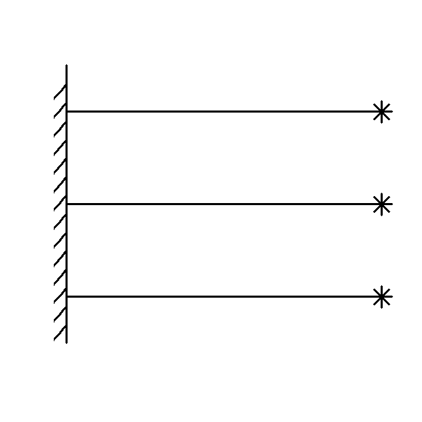
(a)

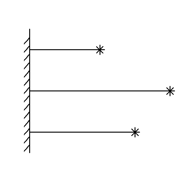
(b)

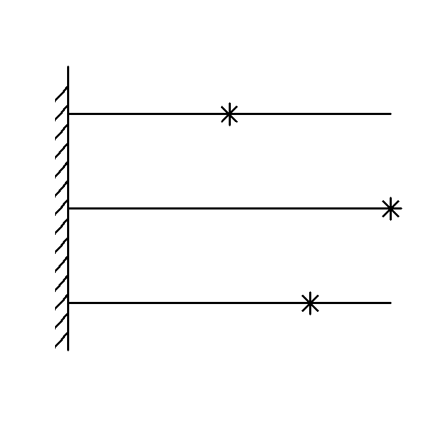
(c)

Figure 1: Schematic depiction of three setups for sequential multiple testing when data are generated by distinct sources. Each horizontal line segment represents the time span of sampling from the corresponding data source and $*$ the decision time for the corresponding testing problem.

In both these setups, sampling is terminated in a data stream as soon as the decision is made for the corresponding testing problem. The difference is that in the first one the decision times must coincide, whereas in the second they may differ. As a result, the first setup is suitable when an action needs to be taken based on the decisions for all testing problems, whereas the second when an action must be taken based on the decision for each, individual testing problem.

Our motivation for the present work is the understanding of a third setup, which is schematically depicted in Figure 1.(c). In this one, the decisions for the various testing problems can be made at different times, using data from all streams, which are monitored until all decisions have been made. As a result, this setup is suitable when a timely action needs to be taken based on the decision for each testing problem, but it is not of primary interest, or maybe even possible, to quickly stop sampling from each data source.

For example, suppose that multiple sensors are deployed, each of them monitors a certain environment, and an action needs to be taken in each of these environments depending on the presence or absence of signal in it. In this context, the advantages of asynchronous decisions are obvious, but it may not be convenient, or necessary, to shut down a sensor after its corresponding decision has been made. This can be the case in applications such as missile identification based on radar measurements Almogi-Nadler et al. (2004), spectrum sensing for cognitive radio Gupta and Kumar (2019), intrusion detection in a computer-based system and fraud detection in a commercial organization Chandola et al. (2009). However, apart from a brief discussion in (De and Baron, 2015, Section 2), this very natural setup for sequential multiple testing does not seem to have been studied in the literature.

In the present paper, we (i) propose a general formulation for the sequential multiple testing problem that encompasses all the above setups, (ii) introduce a novel testing procedure that takes advantage of the flexibility of this formulation, (iii) show that this procedure enjoys a general asymptotic optimality property, and (iv) compute its asymptotic gains over synchronous and decentralized procedures.

To be specific, we assume that there are multiple, independent, sequentially monitored data streams, and we consider a binary hypothesis testing problem for each of them. These testing problems are coupled by global, user-specified error constraints. The decisions for the various testing problems can be made at different times, using data from all streams, which can be monitored until all decisions have been made. Thus, all three setups described earlier are included in this general formulation. We introduce a novel, sequential multiple testing procedure that incorporates arbitrary a priori lower and upper bounds on the number of signals, i.e., data streams in which the alternative hypothesis holds. We show that this procedure achieves the optimal expected decision time in every data stream and under every signal configuration to a first-order asymptotic approximation as global error constraints of both types go to zero. This asymptotic optimality property is established under general parametric composite hypotheses, various global error metrics, and weak distributional assumptions that allow for temporal dependence. Moreover, we evaluate the factor by which the expected decision time in each stream increases, asymptotically as the error rates go to zero, when one is limited to decentralized or synchronous procedures. Finally, we compute in various simulation studies the relative efficiencies of two existing sequential multiple testing procedures over the proposed, and compare them with their limiting values that are obtained from the asymptotic theory.

The remainder of this paper is organized as follows: We formulate the sequential multiple testing problem that we consider in this work in Section 2. We introduce and analyze the proposed procedure, contrasting it with existing procedures in the literature, in Sections 3 and 4. We establish our asymptotic optimality theory in Section 5 and present the results of various simulation studies in Section 6. We extend our methodology and theoretical results to general parametric composite hypotheses in Section 7 and to various error metrics in Section 8. We conclude in Section 9. The proofs of all main results, as well as several supporting lemmas, are presented in Appendices A-E.

We end this introductory section with some notations that we use throughout the paper. We set $\mathbb{N}\equiv\{1,2,\ldots\}$ and, for any $n\in\mathbb{N}$, $[n]\equiv\{1,\ldots,n\}$. For a set $A$, we denote by $2^{A}$ its power set, by $|A|$ its size, and by $\mathbf{1}\{A\}$ its indicator function. For any real numbers $x,y$, we set $x\wedge y\equiv\min\{x,y\}$ and $x\vee y\equiv\max\{x,y\}$. For any sequences of positive real numbers $(x_{n})$ and $(y_{n})$, $x_{n}\sim y_{n}$ stands for $\lim_{n}(x_{n}/y_{n})=1$, $x_{n}\gtrsim y_{n}$ for $\liminf_{n}(x_{n}/y_{n})\geq 1$, $x_{n}\lesssim y_{n}$ for $\limsup_{n}(x_{n}/y_{n})\leq 1$, and $x_{n}\lesssim O(y_{n})$ means that there exists a $C\in\mathbb{R}$ so that $x_{n}\leq Cy_{n}$ for all $n\in\mathbb{N}$. Finally, the minimum or infimum over the empty set is understood as $\infty$.

2 Problem formulation

We consider $K$ data sources that generate independent streams of observations,

$$X_{k}\equiv\{X_{k}(n),\,n\in\mathbb{N}\},\quad k\in[K].$$

For each $n\in\mathbb{N}$ and $k\in[K]$, we denote by $\mathcal{F}_{k}(n)$ the $\sigma$-algebra generated by the observations in stream $k$ up to time $n$, and by $\mathcal{F}(n)$ the $\sigma$-algebra generated by the observations in all streams up to time $n$, i.e.,

$$\mathcal{F}_{k}(n)\equiv\sigma\left(X_{k}(t),\,t\in[n]\right),\quad\mathcal{F}(n)\equiv\sigma\left(\mathcal{F}_{k}(n),\,k\in[K]\right).$$

For each $k\in[K]$, we denote by $\mathrm{P}_{k}$ the distribution of $X_{k}$, consider two hypotheses for it,

$$\mathrm{P}_{k}\in\mathcal{P}_{k}^{0}\quad\text{ versus }\quad\mathrm{P}_{k}\in\mathcal{P}_{k}^{1},$$ (2.1)

and refer to the $k^{th}$ data source as signal if $\mathrm{P}_{k}\in\mathcal{P}_{k}^{1}$ and as noise if $\mathrm{P}_{k}\in\mathcal{P}_{k}^{0}$.

The true subset of signals is unknown and deterministic, but we allow for incorporation of information about it by assuming that it is a priori known to belong to some class, $\Pi$, of subsets of $[K]$. Without loss of generality, we assume that

$$\forall\,k\in[K]\quad\exists\,A,B\in\Pi\quad\text{such that}\quad k\in A\text{ and }k\notin B.$$ (2.2)

When, in particular, a lower bound, $l$, and an upper bound, $u$, are given on the true number of signals, where

$$0\leq l\leq u\leq K,\quad u>0,\quad l<K,$$ (2.3)

we set $\Pi=\Pi_{l,u}$, where

$$\Pi_{l,u}\equiv\{A\subseteq[K]:l\leq|A|\leq u\}.$$

In what follows, when referring to $\Pi$ we assume that (2.2) holds, and when referring to $\Pi_{l,u}$ we assume that (2.3) holds.

To solve the above multiple hypothesis testing problem, we need to determine two vectors,

$$\mathbf{T}\equiv(T_{1},\ldots,T_{K}),\quad\mathbf{D}\equiv(D_{1},\ldots,D_{K}),$$

where, for each $k\in[K]$,

• $T_{k}$ is a random time, taking values in $\mathbb{N}$, at which the decision is made for the testing problem in stream $k$,

• $D_{k}$ is a Bernoulli random variable such that stream $k$ is identified as a signal at time $T_{k}$ if and only if $D_{k}=1$.

With an abuse of notation, we also denote by $\mathbf{D}$ the subset of streams that are identified as signals, i.e.,

$$\mathbf{D}\equiv\{k\in[K]:D_{k}=1\}.$$

We assume that each decision time and each selected hypothesis can depend on the already collected observations from all data streams. Thus, we say that $\chi\equiv(\mathbf{T},\mathbf{D})$ is a sequential multiple testing procedure if, for each $k\in[K]$,

• $T_{k}$ is a stopping time with respect to $\{\mathcal{F}(n),n\in\mathbb{N}\}$,

• $D_{k}$ is an $\mathcal{F}(T_{k})$-measurable Bernoulli random variable,

i.e., for each $n\in\mathbb{N}$ and $i\in\{0,1\}$,

$$\{T_{k}=n\},\;\{T_{k}=n,\,D_{k}=i\}\in\mathcal{F}(n).$$

We refer to such a sequential multiple testing procedure as synchronous if all decisions occur at the same time, i.e.,

$$T_{1}=\cdots=T_{K},$$

and as decentralized if each decision time and each selected hypothesis can depend on the already collected observations only from the corresponding data stream. That is, we say that $\chi\equiv(\mathbf{T},\mathbf{D})$ is decentralized if, for each $k\in[K]$,

• $T_{k}$ is a stopping time with respect to $\{\mathcal{F}_{k}(n),n\in\mathbb{N}\}$,

• $D_{k}$ is an $\mathcal{F}_{k}(T_{k})$-measurable Bernoulli random variable,

i.e., for each $n\in\mathbb{N}$ and $i\in\{0,1\}$,

$$\{T_{k}=n\},\;\{T_{k}=n,\,D_{k}=i\}\in\mathcal{F}_{k}(n).$$

We denote by $\Delta$ the family of all sequential multiple testing procedures, by $\Delta^{\prime}$ the subfamily of decentralized procedures, and by $\Delta^{\prime\prime}$ the subfamily of synchronous procedures. We will further focus on sequential multiple testing procedures that satisfy user-specified bounds on certain metrics for the false positive and the false negative error rates. To simplify the presentation, we consider first the case of simple hypotheses and classical familywise error rates, and we extend the formulation and all subsequent results to general parametric composite hypotheses and to various other error metrics in Sections 7 and 8, respectively. Therefore, until then, we assume that the hypotheses in (2.1) are of the form

$$\mathcal{P}_{k}^{i}=\{\mathrm{P}_{k}^{i}\},\quad i\in\{0,1\},\quad k\in[K]$$

and, for any $A\in\Pi$, we denote by $\mathrm{P}_{A}$ the joint distribution of $(X_{1},\ldots,X_{k})$ when the subset of signals is $A$, i.e.,

$$\mathrm{P}_{A}\equiv\mathrm{P}_{1}\otimes\cdots\otimes\mathrm{P}_{K},\quad\text{where}\quad\mathrm{P}_{k}=\begin{cases}\begin{aligned} &\mathrm{P}_{k}^{0},\;&&\text{if }k\notin A\\ &\mathrm{P}_{k}^{1},\;&&\text{if }k\in A,\end{aligned}\end{cases}$$ (2.4)

and by $\mathrm{E}_{A}$ the corresponding expectation. Moreover, for a sequential multiple testing procedure $\chi\equiv(\mathbf{T},\mathbf{D})\in\Delta$ that terminates almost surely in every stream when the true subset of signals is $A$, i.e.,

$$\mathrm{P}_{A}(T_{k}<\infty)=1,\quad\forall\;k\in[K],$$ (2.5)

we denote by $\text{FWE}_{A}^{1}(\chi)$ its type-I familywise error rate, i.e., the probability of at least one noise being identified as signal, when the true subset of signals is $A$,

$$\text{FWE}_{A}^{1}(\chi)\equiv\mathrm{P}_{A}(\mathbf{D}\backslash A\neq\emptyset)=\mathrm{P}_{A}(\exists\;j\notin A:D_{j}=1),$$ (2.6)

and by $\text{FWE}_{A}^{2}(\chi)$ its type-II familywise error rate, i.e., the probability of at least one signal being identified as noise, when the true subset of signals is $A$,

$$\text{FWE}_{A}^{2}(\chi)\equiv\mathrm{P}_{A}(A\backslash\mathbf{D}\neq\emptyset)=\mathrm{P}_{A}(\exists\;i\in A:D_{i}=0).$$ (2.7)

Thus, for any class of prior information $\Pi$ and any $\alpha,\beta\in(0,1)$,

$$\Delta(\alpha,\beta,\Pi)\equiv\bigg{\{}\chi\in\Delta:\text{FWE}_{A}^{1}(\chi) \leq\alpha\;\;\&\;\;\text{FWE}_{A}^{2}(\chi)\leq\beta,\;\forall\,A\in\Pi\bigg{\}}$$ (2.8)

is the family of sequential multiple testing procedures that control, under every signal configuration consistent with $\Pi$, the type-I and type-II familywise error rates below $\alpha$ and $\beta$, respectively, and

$$\mathcal{L}_{k,A}(\alpha,\beta,\Pi)\equiv\inf\left\{\mathrm{E}_{A}[T_{k}]:(\mathbf{T},\mathbf{D})\in\Delta(\alpha,\beta,\Pi)\right\}$$ (2.9)

is the optimal in $\Delta(\alpha,\beta,\Pi)$ expected decision time in stream $k\in[K]$ when the subset of signals is $A\in\Pi$.

The first goal of the present work is to introduce a testing procedure that achieves (2.9) to a first-order asymptotic approximation as $\alpha$ and $\beta$ go to 0, simultaneously for every $A\in\Pi$ and $k\in[K]$, when $\Pi$ is of the form $\Pi_{l,u}$. The second goal is to quantify the asymptotic gains of the proposed procedure over decentralized and synchronous procedures. Specifically, for any $A\in\Pi$, $k\in[K]$, $\alpha,\beta\in(0,1)$, we consider the optimal expected decision time in stream $k$ when the subset of signals is $A$ in the subfamily of decentralized procedures in $\Delta(\alpha,\beta,\Pi)$, i.e.,

$$\mathcal{L}^{\prime}_{k,A}(\alpha,\beta,\Pi)\equiv\inf\left\{\mathrm{E}_{A}[T_{k}]:(\mathbf{T},\mathbf{D})\in\Delta^{\prime}\cap\Delta(\alpha,\beta,\Pi)\right\},$$ (2.10)

and the optimal expected decision time when the subset of signals is $A$ in the subfamily of synchronous procedures in $\Delta(\alpha,\beta,\Pi)$, i.e.,

$$\mathcal{L}^{\prime\prime}_{A}(\alpha,\beta,\Pi) \equiv\inf\left\{\mathrm{E}_{A}[T_{1}]:(\mathbf{T},\mathbf{D})\in\Delta^{\prime\prime}\cap\Delta(\alpha,\beta,\Pi)\right\}.$$ (2.11)

Our second goal is to evaluate, for any $A\in\Pi_{l,u}$ and $k\in[K]$, the asymptotic relative efficiencies

$$\operatorname{ARE}^{\prime}_{k,A}(l,u) \equiv\lim_{\alpha,\beta\to 0}\frac{\mathcal{L}_{k,A}(\alpha,\beta,\Pi_{l,u})}{\mathcal{L}^{\prime}_{k,A}(\alpha,\beta,\Pi_{l,u})},$$ (2.12)

$$\operatorname{ARE}^{\prime\prime}_{k,A}(l,u) \equiv\lim_{\alpha,\beta\to 0}\frac{\mathcal{L}_{k,A}(\alpha,\beta,\Pi_{l,u})}{\mathcal{L}^{\prime\prime}_{A}(\alpha,\beta,\Pi_{l,u})},$$ (2.13)

where the inverse of (2.12) (resp. (2.13)) represents the limiting value as $\alpha,\beta\to 0$ of the factor by which the best possible expected decision time in stream $k$ when the subset of signals is $A\in\Pi_{l,u}$ increases when allowing only for decentralized (resp. synchronous) procedures in $\Delta(\alpha,\beta,\Pi)$.

2.1 Distributional assumptions

For each $k\in[K]$ and $n\in\mathbb{N}$, we assume that the probability measures $\mathrm{P}_{k}^{1}$ and $\mathrm{P}_{k}^{0}$ are mutually absolutely continuous when restricted to $\mathcal{F}_{k}(n)$, and denote by $\lambda_{k}(n)$ the corresponding log-likelihood ratio (LLR), i.e.,

$$\lambda_{k}(n)\equiv\log\frac{d\mathrm{P}_{k}^{1}}{d\mathrm{P}_{k}^{0}}\left(\mathcal{F}_{k}(n)\right).$$ (2.14)

For the proposed test to terminate with probability 1 and to achieve the prescribed error control, it suffices to assume that, for each $k\in[K]$,

$$\begin{split}\mathrm{P}_{k}^{1}\left(\lim_{n\to\infty}\lambda_{k}(n)=\infty\right)&=1\\ \mathrm{P}_{k}^{0}\left(\lim_{n\to\infty}\lambda_{k}(n)=-\infty\right)&=1.\end{split}$$ (2.15)

To establish our asymptotic optimality theory, we need to make some further distributional assumptions. Specifically, we assume that for each $k\in[K]$ there are positive numbers, $I_{k}$ and $J_{k}$, so that

$$\mathrm{P}_{k}^{1}\left(\limsup_{n\to\infty}\frac{\lambda_{k}(n)}{n}\leq I_{k}\right) =1$$ (2.16)

$$\mathrm{P}_{k}^{0}\left(\limsup_{n\to\infty}\frac{-\lambda_{k}(n)}{n}\leq J_{k}\right) =1,$$

and

$$\begin{split}\forall\;\epsilon>0\quad\sum_{n=1}^{\infty}\mathrm{P}_{k}^{1}\left(\frac{\lambda_{k}(n)}{n}\leq I_{k}-\epsilon\right)&<\infty\\ \forall\;\epsilon>0\quad\sum_{n=1}^{\infty}\mathrm{P}_{k}^{0}\left(\frac{-\lambda_{k}(n)}{n}\leq J_{k}-\epsilon\right)&<\infty.\end{split}$$ (2.17)

Remark 2.1.

By the Borel-Cantellil lemma, condition (2.17) implies

$$\mathrm{P}_{k}^{1}\left(\liminf_{n\to\infty}\frac{\lambda_{k}(n)}{n}\geq I_{k}\right) =1$$

$$\mathrm{P}_{k}^{0}\left(\liminf_{n\to\infty}\frac{-\lambda_{k}(n)}{n}\geq J_{k}\right) =1.$$

Therefore, conditions (2.16)-(2.17) imply

$$\mathrm{P}_{k}^{1}\left(\lim_{n\to\infty}\frac{\lambda_{k}(n)}{n}=I_{k}\right) =1$$ (2.18)

$$\mathrm{P}_{k}^{0}\left(\lim_{n\to\infty}\frac{\lambda_{k}(n)}{n}=-J_{k}\right) =1,$$

and, as a result, they characterize $I_{k}$ and $J_{k}$.

Remark 2.2.

In the special case that $\{\lambda_{k}(n),\,n\in\mathbb{N}\}$ has i.i.d. increments with mean $I_{k}>0$ under $\mathrm{P}_{1}^{k}$ and $-J_{k}<0$ under $\mathrm{P}_{0}^{k}$, by Kolmogorov’s Strong Law of Large Numbers and Chernoff’s bound it follows that conditions (2.16)-(2.17) are equivalent to (2.18) and are automatically satisfied.

2.2 Notations

For any $A\subseteq[K]$, we denote by $\mathcal{I}_{A}$ and $\mathcal{J}_{A}$ the minimum of the numbers in $\{I_{i}:i\in A\}$ and $\{J_{j}:j\notin A\}$, respectively, i.e.,

$$\mathcal{I}_{A}\equiv\min_{i\in A}I_{i}\qquad\text{and}\qquad\mathcal{J}_{A}\equiv\min_{j\notin A}J_{j}.$$ (2.19)

We denote the LLRs at time $n\in\mathbb{N}$ in non-increasing order as $\lambda_{(k)}(n)$, $k\in[K]$, i.e.,

$$\lambda_{(1)}(n)\geq\lambda_{(2)}(n)\geq\cdots\geq\lambda_{(K)}(n),$$

where ties are ordered arbitrarily. Moreover, we denote by $p(n)$ the number of positive LLRs at time $n$, i.e.,

$$p(n)\equiv\big{|}\left\{k\in[K]:\lambda_{k}(n)>0\right\}\big{|}.$$

3 The proposed sequential multiple testing procedure

In this section we introduce the sequential multiple testing procedure that we propose in this work, contrasting it with two existing procedures in the literature, a decentralized one and a synchronous one.

3.1 A decentralized procedure (parallel SPRT)

When considering the binary sequential testing problem in stream $k$ locally, the most natural sequential test is arguably Wald’s Sequential Probability Ratio Test (SPRT),

$$\tilde{T}_{k} \equiv\inf\left\{n\in\mathbb{N}:\lambda_{k}(n)\notin(-b,a)\right\},$$ (3.1)

$$\tilde{D}_{k} \equiv 1\{\lambda_{k}(\tilde{T}_{k})\geq a\big{\}},$$

where $a,b>0$ are thresholds to be determined. Thus, a natural sequential multiple testing procedure is to simply apply an SPRT to each binary testing problem, i.e., $\tilde{\chi}\equiv(\tilde{\mathbf{T}},\tilde{\mathbf{D}})$, where

$$\tilde{\mathbf{T}} \equiv(\tilde{T}_{1},\ldots,\tilde{T}_{K}),$$ (3.2)

$$\tilde{\mathbf{D}} \equiv(\tilde{D}_{1},\ldots,\tilde{D}_{K}).$$

This procedure has been considered, at least as a competitor, in various works (e.g., De and Baron (2012a); Malloy and Nowak (2014); Song and Fellouris (2017); Xing and Fellouris (2022)). It is clearly decentralized and, as we will see in Section 5, it achieves asymptotic optimality in the subfamily of decentralized procedures for any given class of prior information, $\Pi$. However, it does not preserve this asymptotic optimality property in the general family of sequential multiple testing procedures considered in this work when $\Pi$ is of the form $\Pi_{l,u}$ apart from the case of no prior information $(l=0,u=K)$.

3.2 The proposed procedure

Suppose that we are given bounds on the number of signals, i.e., $\Pi$ is of the form $\Pi_{l,u}$. Then, the proposed procedure, $\hat{\chi}\equiv(\hat{\mathbf{T}},\hat{\mathbf{D}})$, is defined as follows:

$$\hat{\mathbf{T}} \equiv(\hat{T}_{1},\ldots,\hat{T}_{K}),\text{ where }\hat{T}_{k}\equiv\hat{T}_{k,1}\wedge\hat{T}_{k,2},\;\;k\in[K],$$ (3.3)

$$\hat{\mathbf{D}} \equiv\big{\{}k\in[K]:\hat{T}_{k}=\hat{T}_{k,1}\big{\}},$$

and the form of $\hat{T}_{k,1}$ and $\hat{T}_{k,2}$ depends on whether $l=u$ or $l<u$. When the number of signals is a priori known to be equal to some $1\leq m\leq K-1$, i.e., $l=u\equiv m$, we set

$$\hat{T}_{k,1} \equiv\inf\left\{n\in\mathbb{N}:\lambda_{k}(n)\geq\lambda_{(m+1)}(n)+c\right\},$$ (3.4)

$$\hat{T}_{k,2} \equiv\inf\left\{n\in\mathbb{N}:\lambda_{k}(n)\leq\lambda_{(m)}(n)-d\right\},$$

where $c,d>0$ are thresholds to be determined. When the number of signals is not a priori known, i.e., $l<u$, we combine the stopping rules in (3.1) and (3.4) and set

$$\hat{T}_{k,1} \equiv\inf\left\{n\in\mathbb{N}:\lambda_{k}(n)\geq\min\{a,\;\lambda_{(l+1)}(n)+c\}\right\},$$ (3.5)

$$\hat{T}_{k,2} \equiv\inf\left\{n\in\mathbb{N}:\lambda_{k}(n)\leq\max\{-b,\;\lambda_{(u)}(n)-d\}\right\},$$

where $a,b,c,d>0$ are again thresholds to be determined.

In the case of no prior information ($l=0$ and $u=K$), thresholds $c$ and $d$ are inactive and $\hat{\chi}$ reduces to the parallel SPRT, introduced in (3.1)-(3.2), as it is not possible, for any $c,d>0$, $k\in[K]$, $n\in\mathbb{N}$, to have

$$\lambda_{k}(n)\geq\lambda_{(1)}(n)+c\qquad\text{or}\qquad\lambda_{k}(n)\leq\lambda_{(K)}(n)-d.$$

On the other hand, in the presence of non-trivial a priori bounds on the number of signals, i.e., when either $l>0$ or $u<K$, $\hat{\chi}$ is not decentralized, as it requires comparisons between statistics of different streams. Indeed, according to this scheme, when $l>0$ (resp. $u<K$), a decision can be made in a stream once its LLR statistic is sufficiently larger (resp. smaller) than the $(l+1)$-th (resp. $u$-th) largest LLR.

3.3 A synchronous procedure

Assuming that $\Pi$ is of the form $\Pi_{l,u}$, the synchronous procedure, $\check{\chi}\equiv(\check{T},\check{\mathbf{D}}),$ in Song and Fellouris (2017) is defined as follows:

• When $l=u\equiv m$,

  $$\check{T}\equiv\inf\left\{n\in\mathbb{N}:\lambda_{(m)}(n)-\lambda_{(m+1)}(n)\geq c\vee d\right\},$$ (3.6)

  where $c,d>0$ are thresholds to be determined, and $\check{\mathbf{D}}$ is the subset of the $m$ streams with the largest LLRs at time $\check{T}$.

• When $l<u$,

  $$\begin{split}\check{T}&\equiv\tau_{1}\wedge\tau_{2}\wedge\tau_{3},\quad\text{where}\\ \tau_{1}&\equiv\inf\left\{n\in\mathbb{N}:\lambda_{(l+1)}(n)\leq\min\{-b,-c+\lambda_{(l)}(n)\}\right\}\\ \tau_{2}&\equiv\inf\left\{n\in\mathbb{N}:\lambda_{k}(n)\notin(-b,a)\;\;\forall\,k\in[K],\text{ and }l\leq p(n)\leq u\right\}\\ \tau_{3}&\equiv\inf\left\{n\in\mathbb{N}:\lambda_{(u)}(n)\geq\max\{a,\,d+\lambda_{(u+1)}(n)\}\right\},\end{split}$$ (3.7)

  where $a,b,c,d>0$ are thresholds to be determined, and $\check{\mathbf{D}}$ is the subset of the $\left(p(\check{T})\vee l\right)\wedge u$ streams with the largest LLRs at time $\check{T}$.
  

In the case of no prior information ($l=0$ and $u=K$),

$$\check{T} =\inf\left\{n\in\mathbb{N}:\lambda_{k}(n)\notin(-b,a)\;\;\forall\,k\in[K]\right\},$$

and $\check{\mathbf{D}}$ is the subset of streams with positive LLRs at time $\check{T}$. Therefore, in this case, $\check{\chi}$ reduces to the Intersection rule introduced in De and Baron (2012a) and makes its decisions once all LLRs are simultaneously outside the interval $(-b,a)$. Clearly, this is never sooner than the last decision time of the parallel SPRT with the same thresholds, $a$ and $b$. In general, for any $l$ and $u$, the last decision time of the proposed procedure occurs no later than the decision time of this synchronous procedure, i.e.,

$$\max_{k\in[K]}\hat{T}_{k}\leq\check{T},\quad\forall\;k\in[K],$$ (3.8)

when the two procedures use the same thresholds $a,b,c,d$.

In Song and Fellouris (2017) it was shown, in the case that each data stream consists of i.i.d. observations, that $\check{\chi}$ is asymptotically optimal in the subfamily of synchronous procedures, i.e., it achieves (2.11) asymptotically as $\alpha,\beta\to 0$ for every $A\in\Pi_{l,u}$. In Section 5 we show that this asymptotic optimality property holds under the general distributional assumptions of Subection 2.1, but does not extend, apart from a very specific setup, to the general family of sequential multiple testing procedures that we consider in this work.

4 Analysis

In this section, we show how the thresholds of the proposed procedure can be selected in order to control the two types of familywise error rates below arbitrary prescribed levels. Moreover, we establish asymptotic upper bounds on its expected decision times in each stream as its thresholds go to infinity. For comparison purposes, we also include the corresponding results for the parallel SPRT and the synchronous procedure introduced in the previous section.

4.1 Error control

Proposition 4.1.

Suppose that (2.15) holds for every $k\in[K]$ and let $A\subseteq[K]$, $a,b,c,d>0$. Then

$$\text{FWE}_{A}^{1}(\tilde{\chi}) \leq|A^{c}|\,e^{-a},$$ (4.1)

$$\text{FWE}_{A}^{2}(\tilde{\chi}) \leq|A|\,e^{-b}.$$ (4.2)

If, also, $\Pi=\Pi_{l,u}$ and $A\in\Pi_{l,u}$, then we have the following:

• If $l=u\equiv m$, then

  $$\text{FWE}_{A}^{1}(\hat{\chi}) \leq m(K-m)\,e^{-c},$$ (4.3)

  $$\text{FWE}_{A}^{2}(\hat{\chi}) \leq m(K-m)\,e^{-d},$$ (4.4)

  $$\text{FWE}_{A}^{1}(\check{\chi})=\text{FWE}_{A}^{2}(\check{\chi}) \leq m(K-m)\,e^{-c\vee d}.$$ (4.5)

• If $l<u$, then

  $$\text{FWE}_{A}^{1}(\hat{\chi}),\;\text{FWE}_{A}^{1}(\check{\chi})\leq|A^{c}|\,(e^{-a}+|A|\,e^{-c}),$$ (4.6)

  $$\text{FWE}_{A}^{2}(\hat{\chi}),\;\text{FWE}_{A}^{2}(\check{\chi})\leq|A|\,(e^{-b}+|A^{c}|\,e^{-d}).$$ (4.7)

Proof.

See Appendix B.
∎

The previous proposition provides a concrete selection for thresholds that guarantee prescribed familywise error rates. Indeed, let $\alpha,\beta\in(0,1)$. Then, for any given $\Pi\subseteq 2^{[K]}$, we have $\tilde{\chi}\in\Delta(\alpha,\beta,\Pi)$ when

$$\begin{split}a&=|\log\alpha|+\max_{A\in\Pi}\,\log|A^{c}|\\ b&=|\log\beta|+\max_{A\in\Pi}\,\log|A|.\end{split}$$ (4.8)

Similarly, for any given $l,u$, we have the following:

• If $l=u\equiv m$, then $\hat{\chi}$ and $\check{\chi}$ both belong to $\Delta(\alpha,\beta,\Pi_{l,u})$ when

  $$\begin{split}c&=|\log\alpha|+\log(m(K-m))\\ d&=|\log\beta|+\log(m(K-m)).\end{split}$$ (4.9)

• If $l<u$, then $\hat{\chi}$ and $\check{\chi}$ both belong to $\Delta(\alpha,\beta,\Pi_{l,u})$ when

  $$\begin{split}a&=|\log\alpha|+\log K\\ b&=|\log\beta|+\log K\\ c&=|\log\alpha|+\log((K-l)\,K)\\ d&=|\log\beta|+\log(u\,K).\end{split}$$ (4.10)

These thresholds suffice for the asymptotic optimality theory we develop in the next section, however they can be quite conservative for practical use. Alternatively, one may use Monte Carlo simulation to determine the thresholds that equate, at least approximately, the maximum familywise error rates to their target levels. When the target levels are very small, this can be done efficiently using importance sampling, as we discuss in Subsection 6.2.

Proposition 4.2.

Suppose that (2.17) holds and let $A\subseteq[K]$, $i\in A$, $j\notin A$. Then, as $a,b\to\infty$,

$$\mathrm{E}_{A}[\tilde{T}_{i}]\lesssim\frac{a}{I_{i}}\qquad\text{and}\qquad\mathrm{E}_{A}[\tilde{T}_{j}]\lesssim\frac{b}{J_{j}}.$$ (4.11)

If, also, $\Pi=\Pi_{l,u}$ and $A\in\Pi_{l,u}$, then we have the following:

• If $l=u$, then, as $c,d\to\infty$,

  $$\mathrm{E}_{A}[\hat{T}_{i}]\lesssim\frac{c}{I_{i}+\mathcal{J}_{A}},\qquad\mathrm{E}_{A}[\hat{T}_{j}]\lesssim\frac{d}{J_{j}+\mathcal{I}_{A}},$$ (4.12)

  $$\mathrm{E}_{A}[\check{T}]\lesssim\frac{c\vee d}{\mathcal{I}_{A}+\mathcal{J}_{A}}.$$ (4.13)

• If $l<u$, then, as $a,b,c,d\to\infty$,

  $$\mathrm{E}_{A}[\hat{T}_{i}] \lesssim\begin{cases}\begin{aligned} &\frac{a}{I_{i}}\wedge\frac{c}{I_{i}+\mathcal{J}_{A}},&&\text{if }|A|=l\\ &\;\;\frac{a}{I_{i}},&&\text{if }l<|A|\leq u,\end{aligned}\end{cases}$$ (4.14)

  $$\mathrm{E}_{A}[\hat{T}_{j}] \lesssim\begin{cases}\begin{aligned} &\;\;\frac{b}{J_{j}},&&\text{if }l\leq|A|<u\\ &\frac{b}{J_{j}}\wedge\frac{d}{J_{j}+\mathcal{I}_{A}},&&\text{if }|A|=u,\end{aligned}\end{cases}$$

  and

  $$\mathrm{E}_{A}[\check{T}]\lesssim\begin{cases}\begin{aligned} &\max\left\{\frac{b}{\mathcal{J}_{A}},\;\frac{a}{\mathcal{I}_{A}}\wedge\frac{c}{\mathcal{I}_{A}+\mathcal{J}_{A}}\right\},&&\text{if }|A|=l\\ &\max\left\{\frac{a}{\mathcal{I}_{A}},\;\frac{b}{\mathcal{J}_{A}}\right\},&&\text{if }l<|A|<u\\ &\max\left\{\frac{a}{\mathcal{I}_{A}},\;\frac{b}{\mathcal{J}_{A}}\wedge\frac{d}{\mathcal{J}_{A}+\mathcal{I}_{A}}\right\},&&\text{if }|A|=u.\end{aligned}\end{cases}$$ (4.15)

  In particular, as $a,b,c,d\to\infty$ so that $a\sim c$ and $b\sim d$,

  $$\mathrm{E}_{A}[\hat{T}_{i}] \lesssim\frac{a}{I_{i}+\mathcal{J}_{A}\cdot\mathbf{1}\{|A|=l\}},$$ (4.16)

  $$\mathrm{E}_{A}[\hat{T}_{j}] \lesssim\frac{b}{J_{j}+\mathcal{J}_{A}\cdot\mathbf{1}\{|A|=u\}},$$

  and

  $$\mathrm{E}_{A}[\check{T}]\lesssim\max\left\{\frac{a}{\mathcal{I}_{A}+\mathcal{J}_{A}\cdot\mathbf{1}\{|A|=l\}},\;\frac{b}{\mathcal{J}_{A}+\mathcal{I}_{A}\cdot\mathbf{1}\{|A|=u\}}\right\}.\\$$ (4.17)

Proof.

See Appendix B.
∎

The above first-order asymptotic upper bounds are free of $l$ and $u$. In the next proposition we consider an i.i.d. setup and obtain second-order terms that depend on $l$ (resp. $u$) when the true number of signals is $l$ (resp. $u$).

Proposition 4.3.

Suppose that the increments of $\{\lambda_{k}(n),n\in\mathbb{N}\}$ are i.i.d. with finite variance and mean $I_{k}>0$ under $\mathrm{P}_{k}^{1}$ and $-J_{k}<0$ under $\mathrm{P}_{k}^{0}$ for every $k\in[K]$. Let $A\subseteq[K]$, $i\in A$, $j\notin A$. Then, as $a,b\to\infty$,

$$\mathrm{E}_{A}[\tilde{T}_{i}]\leq\frac{a}{I_{i}}+O(1)\qquad\text{and}\qquad\mathrm{E}_{A}[\tilde{T}_{j}]\leq\frac{b}{J_{j}}+O(1).$$ (4.18)

If, also, $\Pi=\Pi_{l,u}$ and $A\in\Pi_{l,u}$, then we have the following:

• If $l=u\equiv m$, then, as $c,d\to\infty$,

  $$\mathrm{E}_{A}[\hat{T}_{i}] \leq\frac{c}{I_{i}+\mathcal{J}_{A}}+O\left((K-m)\sqrt{c}\right),$$ (4.19)

  $$\mathrm{E}_{A}[\hat{T}_{j}] \leq\frac{d}{J_{j}+\mathcal{I}_{A}}+O(m\sqrt{d}),$$ (4.20)

  $$\mathrm{E}_{A}[\check{T}] \leq\frac{c\vee d}{\mathcal{I}_{A}+\mathcal{J}_{A}}+O\left(m(K-m)\sqrt{c\vee d}\right).$$ (4.21)

• If $l<u$, then, as $a,b,c,d\to\infty$ so that $|c-a|=O(1)$ and $|d-b|=O(1)$,

  $$\mathrm{E}_{A}[\hat{T}_{i}] \lesssim\begin{cases}\begin{aligned} &\frac{a}{I_{i}+\mathcal{J}_{A}}+O\left((K-l)\sqrt{a}\right),&&\text{if }|A|=l,\\ &\;\;\frac{a}{I_{i}}+O(1),&&\text{if }l<|A|\leq u.\end{aligned}\end{cases}$$ (4.22)

  $$\mathrm{E}_{A}[\hat{T}_{j}] \lesssim\begin{cases}\begin{aligned} &\;\;\frac{b}{J_{j}}+O(1),&&\text{if }l\leq|A|<u,\\ &\frac{b}{J_{j}+\mathcal{I}_{A}}+O(u\sqrt{b}),&&\text{if }|A|=u.\end{aligned}\end{cases}$$ (4.23)

Proof.

See Appendix B.
∎

Remark 4.1.

The upper bounds in (4.19) and (4.22) (resp. (4.20) and (4.23)) suggest that the expected decision time of the proposed test in a signal (resp. noise) stream should be decreasing in $l$ (resp. increasing in $u$) when the true number of signals is $l$ (resp. $u$), and independent of $l$ and $u$ when the true number of signals is larger than $l$ (resp. smaller than $u$). On the other hand, when the number of signals is a priori known i.e., $l=u\equiv m$, the upper bound in (4.21) suggests that the expected decision time of the synchronous test increases as $m$ approaches $K/2$. The intuition from these bounds will be corroborated in the simulation studies of Section 6.

5 Asymptotic optimality

In this section we establish the asymptotic optimality theory of the paper. First, we state a universal, asymptotic (as $\alpha,\beta\to 0$) lower bound on $\mathcal{L}_{k,A}(\alpha,\beta,\Pi)$, defined in (2.9), for any $k\in[K]$, $A\in\Pi$, and any class of prior information $\Pi$, and then we show that it is attained by the proposed procedure simultaneously for every $A\in\Pi$ and $k\in[K]$ when $\Pi$ is of the form $\Pi_{l,u}$.

Lemma 5.1.

Let $\Pi$ satisfy (2.2), $A\in\Pi$, $i\in A$, $j\notin A$. If condition (2.16) holds for every $k\in[K]$, then, as $\alpha,\beta\to 0$,

$$\mathcal{L}_{i,A}(\alpha,\beta,\Pi)\gtrsim\frac{|\log\alpha|}{\min\{I_{A,C}:C\in\Pi,\,i\notin C\}},$$ (5.1)

$$\mathcal{L}_{j,A}(\alpha,\beta,\Pi)\gtrsim\frac{|\log\beta|}{\min\{I_{A,C}:C\in\Pi,\,j\in C\}},$$ (5.2)

where

$$I_{A,C}\equiv\sum_{k\in A\backslash C}I_{k}+\sum_{k\in C\backslash A}J_{k}.$$ (5.3)

Proof.

See Appendix C.
∎

Theorem 5.1.

Let $l,u$ satisfy (2.3). Suppose that the thresholds $a,b,c,d$ of $\hat{\chi}$ are selected so that $\hat{\chi}\in\Delta(\alpha,\beta,\Pi_{l,u})$ for any $\alpha,\beta\in(0,1)$, and also

$$a,c\sim|\log\alpha|\quad\text{and}\quad b,d\sim|\log\beta|\quad\text{as}\quad\alpha,\beta\to 0,$$ (5.4)

e.g., according to (4.9) when $l=u$ and (4.10) when $l<u$.

If conditions (2.16)-(2.17) hold for every $k\in[K]$, then, as $\alpha,\beta\to 0$,

$$\mathrm{E}_{A}[\hat{T}_{i}] \sim\mathcal{L}_{i,A}(\alpha,\beta,\Pi_{l,u})\sim\frac{|\log\alpha|}{I_{i}+\mathcal{J}_{A}\cdot\mathbf{1}\left\{|A|=l\right\}},$$ (5.5)

$$\mathrm{E}_{A}[\hat{T}_{j}] \sim\mathcal{L}_{j,A}(\alpha,\beta,\Pi_{l,u})\sim\frac{|\log\beta|}{J_{j}+\mathcal{I}_{A}\cdot\mathbf{1}\left\{|A|=u\right\}},$$ (5.6)

simultaneously for every $i\in A$, $j\notin A$, $A\in\Pi_{l,u}$.

Proof.

See Appendix C.
∎

5.1 Comparison with decentralized procedures

We next establish the asymptotic optimality of the parallel SPRT, $\tilde{\chi}$, defined in (3.1)-(3.2), in the subfamily of decentralized procedures, for any given class of prior information.

Theorem 5.2.

Let $\Pi$ satisfy (2.2). Suppose that the thresholds $a,b$ of $\tilde{\chi}$ are selected so that $\tilde{\chi}\in\Delta(\alpha,\beta,\Pi)$ for any $\alpha,\beta\in(0,1)$, and also

$$a\sim|\log\alpha|\quad\text{and}\quad b\sim|\log\beta|\quad\text{as}\quad\alpha,\beta\to 0,$$ (5.7)

e.g., according to (4.8).

If conditions (2.16)-(2.17) hold for every $k\in[K]$, then, as $\alpha,\beta\to 0$,

$$\mathrm{E}_{A}[\tilde{T}_{i}] \sim\mathcal{L}^{\prime}_{i,A}(\alpha,\beta,\Pi)\sim\frac{|\log\alpha|}{I_{i}},$$ (5.8)

$$\mathrm{E}_{A}[\tilde{T}_{j}] \sim\mathcal{L}^{\prime}_{j,A}(\alpha,\beta,\Pi)\sim\;\frac{|\log\beta|}{J_{j}},$$

simultaneously for every $i\in A$, $j\notin A$, $A\in\Pi$.

Proof.

See Appendix C.
∎

Using Theorems 5.1 and 5.2 we can now evaluate the asymptotic relative efficiencies in (2.12).

Corollary 5.2.1.

Let $\Pi$ satisfy (2.2). Suppose that conditions (2.16)-(2.17) hold for every $k\in[K]$. Then, for every $i\in A$, $j\notin A$, $A\in\Pi_{l,u}$,

$$\begin{split}\operatorname{ARE}^{\prime}_{i,A}(l,u)&=\begin{cases}\begin{aligned} &I_{i}/(I_{i}+\mathcal{J}_{A}),&&\text{when}\quad|A|=l\\ &1,&&\text{otherwise},\end{aligned}\end{cases}\\ \operatorname{ARE}^{\prime}_{j,A}(l,u)&=\begin{cases}\begin{aligned} &J_{j}/(J_{j}+\mathcal{I}_{A}),&&\text{when}\quad|A|=u\\ &1,&&\text{otherwise}.\end{aligned}\end{cases}\end{split}$$ (5.9)

When, in particular, $l=0$,

$$\operatorname{ARE}^{\prime}_{i,A}(l,u)=1,\quad\forall\;i\in A,$$

and when $u=K$,

$$\operatorname{ARE}^{\prime}_{j,A}(l,u)=1,\quad\forall\;j\notin A.$$

Proof.

It suffices to compare (5.5)-(5.6) and (5.8).
∎

If the multiple testing problem is homogeneous in the sense that

$$I_{k}=I\quad\text{and}\quad J_{k}=J,\quad\forall\;k\in[K],$$ (5.10)

then (5.9) reduces to

$$\begin{split}\operatorname{ARE}^{\prime}_{i,A}(l,u)&=\begin{cases}\begin{aligned} &I/(I+J),&&\text{when}\quad|A|=l\\ &1,&&\text{otherwise},\end{aligned}\end{cases}\\ \operatorname{ARE}^{\prime}_{j,A}(l,u)&=\begin{cases}\begin{aligned} &J/(I+J),&&\text{when}\quad|A|=u\\ &1,&&\text{otherwise}.\end{aligned}\end{cases}\end{split}$$ (5.11)

If the multiple testing problem is also symmetric in the sense that

$$I_{k}=J_{k},\quad\forall\;k\in[K],$$ (5.12)

then

$$\begin{split}\operatorname{ARE}^{\prime}_{i,A}(l,u)&=\begin{cases}\begin{aligned} &1/2,&&\text{when}\quad|A|=l\\ &1,&&\text{otherwise},\end{aligned}\end{cases}\\ \operatorname{ARE}^{\prime}_{j,A}(l,u)&=\begin{cases}\begin{aligned} &1/2,&&\text{when}\quad|A|=u\\ &1,&&\text{otherwise}.\end{aligned}\end{cases}\end{split}$$ (5.13)

Theorems 5.1 and 5.2 and Corollary 5.2.1 imply that when the thresholds of the parallel SPRT and the proposed test are selected so that (5.4) and (5.7) hold, the two tests induce, asymptotically as $\alpha,\beta\to 0$, the same expected decision time in every signal (resp. noise) stream apart from when the true number of signals is equal to its a priori lower (resp. upper) bound. In the latter case, the expected decision time of the parallel SPRT is larger in every signal (resp. noise) stream and, in particular, twice as large when (5.10) and (5.12) hold.

Finally, we stress that the above comparisons are only valid to a first-order asymptotic approximation as $\alpha,\beta\to 0$. The actual, i.e., non-asymptotic, relative efficiencies of the parallel SPRT over the proposed test are computed in various simulation studies in Section 6, where they are compared with their limiting values in (5.9).

5.2 Comparison with synchronous procedures

We next establish the asymptotic optimality of the synchronous procedure, defined in (3.6)-(3.7), in the subfamily of synchronous procedures, extending and generalizing the corresponding result in Song and Fellouris (2017) that applies only to the i.i.d. setup and under a second moment assumption on the log-likelihood ratios.

Theorem 5.3.

Let $l,u$ satisfy (2.3). Suppose that the thresholds $a,b,c,d$ of $\check{\chi}$ are selected so that $\check{\chi}\in\Delta(\alpha,\beta,\Pi_{l,u})$ for any $\alpha,\beta\in(0,1)$ and also so that (5.4) holds.

If conditions (2.16)-(2.17) hold for every $k\in[K]$, then, as $\alpha,\beta\to 0$,

$$\mathrm{E}_{A}[\check{T}] \sim\mathcal{L}^{\prime\prime}_{A}(\alpha,\beta,\Pi_{l,u})$$ (5.14)

$$\sim\max\left\{\frac{|\log\alpha|}{\mathcal{I}_{A}+\mathcal{J}_{A}\cdot\mathbf{1}\left\{|A|=l\right\}},\;\frac{|\log\beta|}{\mathcal{J}_{A}+\mathcal{I}_{A}\cdot\mathbf{1}\left\{|A|=u\right\}}\right\}$$

simultaneously for every $A\in\Pi_{l,u}$.

Proof.

See Appendix C.
∎

From Theorems 5.1 and 5.3 it follows that the optimal expected decision time in the subfamily of synchronous procedures agrees, to a first-order asymptotic approximation as $\alpha,\beta\to 0$, with the maximum (with respect to the streams) optimal expected decision time in the general family of sequential multiple testing procedures. This is the content of the following corollary.

Corollary 5.3.1.

Let $l,u$ satisfy (2.3) and suppose that conditions (2.16)-(2.17) hold for every $k\in[K]$. Then, as $\alpha,\beta\to 0$,

$$\mathcal{L}^{\prime\prime}_{A}(\alpha,\beta,\Pi_{l,u})\sim\max_{k\in[K]}\mathcal{L}_{k,A}(\alpha,\beta,\Pi_{l,u})$$ (5.15)

simultaneously for every $A\in\Pi_{l,u}$.

Proof.

Compare (5.5)-(5.6) and (5.14).
∎

Using Theorems 5.1 and 5.3, we next evaluate the asymptotic relative efficiencies in (2.13).

Corollary 5.3.2.

Let $l,u$ satisfy (2.3), $A\in\Pi_{l,u}$, $i\in A$, $j\notin A$. Suppose that conditions (2.16)-(2.17) hold for every $k\in[K]$.

1. If $\alpha,\beta\to 0$ so that $|\log\alpha|\ll|\log\beta|$, then

   $$\operatorname{ARE}^{\prime\prime}_{i,A}(l,u) =0,$$

   $$\operatorname{ARE}^{\prime\prime}_{j,A}(l,u) =\frac{\mathcal{J}_{A}+\mathcal{I}_{A}\cdot\mathbf{1}\{|A|=u\}}{J_{j}+\mathcal{I}_{A}\cdot\mathbf{1}\{|A|=u\}}.$$

2. If $\alpha,\beta\to 0$ so that $|\log\alpha|\gg|\log\beta|$, then

   $$\operatorname{ARE}^{\prime\prime}_{i,A}(l,u) =\frac{\mathcal{I}_{A}+\mathcal{J}_{A}\cdot\mathbf{1}\{|A|=l\}}{I_{i}+\mathcal{J}_{A}\cdot\mathbf{1}\{|A|=l\}},$$

   $$\operatorname{ARE}^{\prime\prime}_{j,A}(l,u) =0.$$

3. If $\alpha,\beta\to 0$ so that $|\log\alpha|\sim r|\log\beta|$ for some $r>0$, then

   $$\operatorname{ARE}^{\prime\prime}_{i,A}(l,u) =\frac{r/(I_{i}+\mathcal{J}_{A}\cdot\mathbf{1}\{|A|=l\})}{\max\big{\{}r/(\mathcal{I}_{A}+\mathcal{J}_{A}\cdot\mathbf{1}\{|A|=l\}),\,1/(\mathcal{J}_{A}+\mathcal{I}_{A}\cdot\mathbf{1}\{|A|=u\})\big{\}}},$$ (5.16)

   $$\operatorname{ARE}^{\prime\prime}_{j,A}(l,u) =\frac{1/(J_{j}+\mathcal{I}_{A}\cdot\mathbf{1}\{|A|=u\})}{\max\big{\{}r/(\mathcal{I}_{A}+\mathcal{J}_{A}\cdot\mathbf{1}\{|A|=l\}),\,1/(\mathcal{J}_{A}+\mathcal{I}_{A}\cdot\mathbf{1}\{|A|=u\})\big{\}}}.$$

Proof.

Compare (5.5)-(5.6) and (5.14).
∎

Remark 5.1.

Suppose that the multiple testing problem is homogeneous, i.e., (5.10) holds, and also

$$|\log\alpha|\sim|\log\beta|\quad\text{as}\quad\alpha,\beta\to 0.$$ (5.17)

In this case, if the number of signals is a priori known, i.e., $l=u$, then

$$\operatorname{ARE}^{\prime\prime}_{k,A}(l,u)=1,\quad\forall\;k\in[K].$$ (5.18)

On the other hand, if the number of signals is not a priori known, i.e., $l<u$, then

	$|A|=l$	$l<|A|<u$	$|A|=u$
$\operatorname{ARE}^{\prime\prime}_{i,A}(l,u)$	$J/(I+J)$	$(I\wedge J)/I$	1
$\operatorname{ARE}^{\prime\prime}_{j,A}(l,u)$	1	$(I\wedge J)/J$	$I/(I+J)$

Suppose, also, that the multiple testing problem is symmetric, i.e., (5.12) holds, then

$$\begin{split}\operatorname{ARE}^{\prime\prime}_{i,A}(l,u)&=\begin{cases}\begin{aligned} &1/2,&&\text{when}\quad|A|=l<u\\ &1,&&\text{otherwise},\end{aligned}\end{cases}\\ \operatorname{ARE}^{\prime\prime}_{j,A}(l,u)&=\begin{cases}\begin{aligned} &1/2,&&\text{when}\quad|A|=u>l\\ &1,&&\text{otherwise}.\\ \end{aligned}\end{cases}\end{split}$$ (5.19)

Theorems 5.1 and 5.3 and Corollary 5.3.2 imply that when the thresholds of synchronous and the proposed test are selected so that (5.4) holds, then the following hold:

• When $|\log\alpha|$ diverges at a slower (resp. faster) rate than $|\log\beta|$, the expected decision time of the synchronous test is asymptotically much larger than that of the proposed test in a signal (resp. noise) stream and asymptotically larger in noise (resp. signal) stream $j$ (resp. $i$) unless $J_{j}$ (resp. $I_{i}$) is equal to the minimum $\mathcal{J}_{A}$ (resp. $\mathcal{I}_{A}$), defined in (2.19).

• When $|\log\alpha|$ and $|\log\beta|$ are of the same order of magnitude and the multiple testing problem is homogeneous, then the expected decision time of the synchronous test is asymptotically the same as that of the proposed test in every signal (resp. noise) stream when $|A|=u$ (resp. $|A|=l$). When the multiple testing problem is also symmetric, the expected decision time of the synchronous test is asymptotically the same as that of the proposed test in every signal (resp. noise) stream also when $l<|A|<u$, and twice as large when $l=|A|<u$ (resp. $l<|A|=u$).

We reiterate that the above comparisons are valid to a first-order asymptotic approximation as $\alpha,\beta\to 0$. The actual, i.e., non-asymptotic, relative efficiencies of the synchronous test over the proposed test are computed in various simulation studies in Section 6, where they are compared with their limiting values in (5.16).

6 Simulation studies

In this section we compare the proposed test, $\hat{\chi}$, the parallel SPRT, $\tilde{\chi}$, and the synchronous test, $\check{\chi}$, in various simulation studies where each $X_{k}$ is a sequence of i.i.d. Gaussian random variables with variance 1 and mean $0$ (resp. $\mu_{k}$) under $\mathrm{P}_{k}^{0}$ (resp. $\mathrm{P}_{k}^{1}$). Thus, for each $k\in[K]$,

$$\lambda_{k}(n)=\mu_{k}\sum_{i=1}^{n}\big{(}X_{k}(i)-\mu_{k}/2\big{)},\quad n\in\mathbb{N},$$

and conditions (2.16)-(2.17) are satisfied with $I_{k}=J_{k}=\mu_{k}^{2}/2$. Therefore, the multiple testing problem is symmetric, i.e., (5.12) holds, but not necessarily homogeneous. Indeed, we consider two cases for the means under the alternative hypotheses,

• a homogeneous one, where

  $$\mu_{k}=\mu,\quad k\in[K],$$ (6.1)

• and a non-homogeneous one, where there is some $\phi\in(0,1)$ so that

  $$\mu_{k} =\phi\,\mu,\quad 1\leq k\leq K/2,$$ (6.2)

  $$\mu_{k} =\mu,\quad K/2<k\leq K.$$

Moreover, we consider two cases regarding prior information on the number of signals:

• the number of signals is a priori known, i.e., $l=u$,

• the number of signals is at least $l$ and at most $u$ where $l<u$ and $l+u=K$.

6.1 Design

For each of the three tests under consideration, we let only one free parameter for its design. Specifically, for the parallel SPRT we set $a=b$, whereas for the proposed and the synchronous test, we set $c=d$ when $l=u$, and

$$a=b,\quad c=a+\log(K-l),\quad d=b+\log u,\quad\text{when}\quad l<u.$$ (6.3)

For a wide range of values of the free parameter, we compute, for each $A\in\Pi_{l,u}$, the expected decision times in each stream, i.e.,

$$\mathrm{E}_{A}[\hat{T}_{k}],\quad\mathrm{E}_{A}[\tilde{T}_{k}],\quad\mathrm{E}_{A}[\check{T}],\quad\forall\;k\in[K],$$ (6.4)

and the corresponding familywise error rates, i.e.,

$$\text{FWE}_{A}^{i}(\hat{\chi}),\quad\text{FWE}_{A}^{i}(\tilde{\chi}),\quad\text{FWE}_{A}^{i}(\check{\chi}),\quad i\in\{0,1\}.$$ (6.5)

From the latter we obtain the maximum familywise error rates

$$\begin{split}\hat{\alpha}&\equiv\max_{A\in\Pi_{l,u}}\text{FWE}_{A}^{1}(\hat{\chi})\qquad\text{and}\qquad\hat{\beta}\equiv\max_{A\in\Pi_{l,u}}\text{FWE}_{A}^{2}(\hat{\chi}),\\ \tilde{\alpha}&\equiv\max_{A\in\Pi_{l,u}}\text{FWE}_{A}^{1}(\tilde{\chi})\qquad\text{and}\qquad\tilde{\beta}\equiv\max_{A\in\Pi_{l,u}}\text{FWE}_{A}^{2}(\tilde{\chi}),\\ \check{\alpha}&\equiv\max_{A\in\Pi_{l,u}}\text{FWE}_{A}^{1}(\check{\chi})\qquad\text{and}\qquad\check{\beta}\equiv\max_{A\in\Pi_{l,u}}\text{FWE}_{A}^{2}(\check{\chi}).\end{split}$$

6.2 Computation

For the computation of the expected decision times in (6.4) we used plain Monte Carlo, but for the estimation of the familywise error rates in (6.5) we used importance sampling. To be specific, for each $A\in\mathcal{P}_{l,u}$, the familywise error rates of the parallel SPRT are given by

$$\text{FWE}_{A}^{1}(\tilde{\chi}) =1-\prod_{j\notin A}\big{(}1-\mathrm{P}_{j}^{0}(D_{j}=1)\big{)}$$

$$\text{FWE}_{A}^{2}(\tilde{\chi}) =1-\prod_{i\in A}\big{(}1-\mathrm{P}_{i}^{1}(D_{i}=0)\big{)},$$

and it suffices to estimate the error probabilities of the SPRT in each individual testing problem. This can be done using the importance sampling approach described in Siegmund (1976).

A generalization of this importance sampling approach is proposed in (Song and Fellouris, 2017, Section 4) for the estimation of the familywise error rates of the synchronous test, and we follow a similar approach for the estimation of the familywise error rates of the proposed test. To be specific, let us consider the estimation of the type-I familywise error rate under some $A\subseteq[K]$. Then, we select the importance sampling distribution $\mathrm{P}_{A}^{*}$ as in (Song and Fellouris, 2017, Section 4) and we evaluate, via plain Monte Carlo, the right-hand side of the following identity:

$$\text{FWE}_{A}^{1}(\hat{\chi}) \equiv\mathrm{P}_{A}(\hat{\mathbf{D}}\backslash A\neq\emptyset)=\mathrm{E}_{A}^{*}\left[\left(\frac{d\mathrm{P}_{A}^{*}}{d\mathrm{P}_{A}}(\mathcal{F}(\tau_{A}^{1}))\right)^{-1};\;\hat{\mathbf{D}}\backslash A\neq\emptyset\right],$$

where $\tau_{A}^{1}$ is the first time the proposed test commits a type-I error when the true subset of signals is $A$, i.e.,

$$\tau_{A}^{1}\equiv\inf\left\{n\in\mathbb{N}:\exists\,j\notin A,\;\hat{T}_{j}=n\text{ and }\hat{D}_{j}=1\right\}.$$

We note that $\tau_{A}^{1}$ can be replaced in the above identity by $\max_{k\in[K]}\hat{T}_{k}$, but in that case the variance of the resulting estimator increases considerably.

Overall, for the computation of each quantity in (6.4)-(6.5) we used $10^{4}$ Monte Carlo replications and obtained relative errors below $0.5\%$ in all cases.

6.3 Comparisons

For each setup under consideration and each $A\in\Pi_{l,u}$, we plot the expected decision time of each of the three tests in every signal (resp. noise) stream against the absolute value of the base-10 logarithm of the maximum type-I (resp. -II) familywise error rate. That is, for each $i\in A$ we plot

$$\begin{split}\mathrm{E}_{A}[\hat{T}_{i}]\quad\text{against}\quad&|\lg\hat{\alpha}|,\\ \mathrm{E}_{A}[\tilde{T}_{i}]\quad\text{against}\quad&|\lg\tilde{\alpha}|,\\ \mathrm{E}_{A}[\check{T}]\quad\text{against}\quad&|\lg\check{\alpha}|,\end{split}$$ (6.6)

and for each $j\not\in A$ we plot

$$\mathrm{E}_{A}[\hat{T}_{j}]\quad\text{against} |\lg\hat{\beta}|,$$ (6.7)

$$\mathrm{E}_{A}[\tilde{T}_{j}]\quad\text{against} |\lg\tilde{\beta}|,$$

$$\mathrm{E}_{A}[\check{T}]\quad\text{against} |\lg\check{\beta}|.$$

Moreover, we plot the ratios of the expected decision times of the parallel SPRT and of the synchronous test over those of the proposed test in every signal (resp. noise) stream, also against the common absolute value of the base-10 logarithm of the maximum type-I (resp. -II) familywise error rate. That is, for each $i\in A$ we plot

$$\begin{split}\frac{\mathrm{E}_{A}[\hat{T}_{i}]}{\mathrm{E}_{A}[\tilde{T}_{i}]}\;\quad\text{against}\quad&|\lg\hat{\alpha}|=|\lg\tilde{\alpha}|,\\ \frac{\mathrm{E}_{A}[\hat{T}_{i}]}{\mathrm{E}_{A}[\check{T}]}\;\quad\text{against}\quad&|\lg\hat{\alpha}|=|\lg\check{\alpha}|,\end{split}$$ (6.8)

and for each $j\notin A$ we plot

$$\frac{\mathrm{E}_{A}[\hat{T}_{j}]}{\mathrm{E}_{A}[\tilde{T}_{j}]}\quad\text{against} |\lg\hat{\beta}|=|\lg\tilde{\beta}|,$$ (6.9)

$$\frac{\mathrm{E}_{A}[\hat{T}_{j}]}{\mathrm{E}_{A}[\check{T}]}\quad\text{against} |\lg\hat{\beta}|=|\lg\check{\beta}|.$$

Meanwhile, we compare the above relative efficiencies with their limiting values. For the parallel SPRT, they are given by (5.9). For the synchronous test, they are given by (5.16) with $r=1$, since in all cases we consider we have

$$\check{\alpha}=\check{\beta}.$$

Indeed, when $l=u=m$, the decision of the synchronous test, $\check{\mathbf{D}}$, is always of size $m$ and it commits a type-I error if and only if it commits a type-II error. When $l<u$, $\check{\alpha}=\check{\beta}$ holds because the thresholds are selected according to (6.3), $l+u=K$ and

the distribution of $$\lambda_{k} \mathrm{P}_{k}^{1}$$ under is the same as (6.10)

that of $$-\lambda_{k} \text{ $\mathrm{P}_{k}^{0}$, \; for every }k\in[K].$$ under

6.4 Results in the homogeneous setup

We first consider the homogeneous setup, (6.1), with $K=10$, $\mu=0.5$. In this case, the expected decision time is the same in every signal (resp. noise) stream, i.e., (6.6) and (6.8) (resp. (6.7) and (6.9)) do not depend on $i\in A$ (resp. $j\notin A$). Moreover, (6.6) and (6.8) coincide with (6.7) and (6.9) when $l,u,A$ are replaced by $K-u,K-l,A^{c}$. When $l=u$, this is the case because $c=d$ and (6.10) holds. When $l<u$, this is the case because the thresholds are selected according to (6.3), $l+u=K$, and (6.10) holds.

In view of these observations, we only plot (6.6) and (6.8) for an arbitrary $A$ and an arbitrary $i\in A$ when $l=u$ in Figure 2, and for every $|A|\in\{l,\ldots,u\}$ and an arbitrary $i\in A$ when $l<u$ in Figure 3. In each figure, the first row depicts the expected decision time in an arbitrary signal stream, (6.6), and the second row the relative efficiency, (6.8), both against the absolute value of the base-10 logarithm of the maximum type-I familywise error rate. The first column refers to the proposed test, the second to the parallel SPRT, and the third to the synchronous test.

6.4.1 Known number of signals

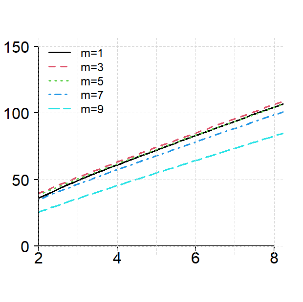
(a) $\hat{\chi}$

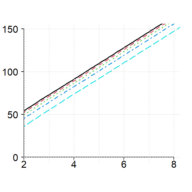
(b) $\tilde{\chi}$

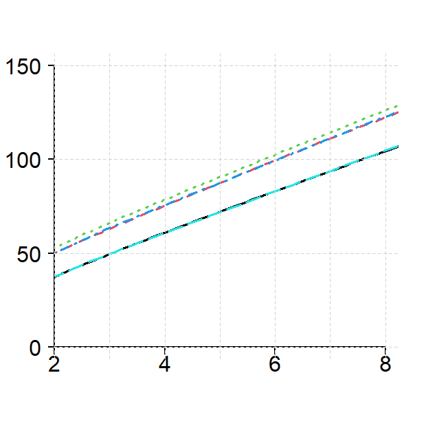
(c) $\check{\chi}$

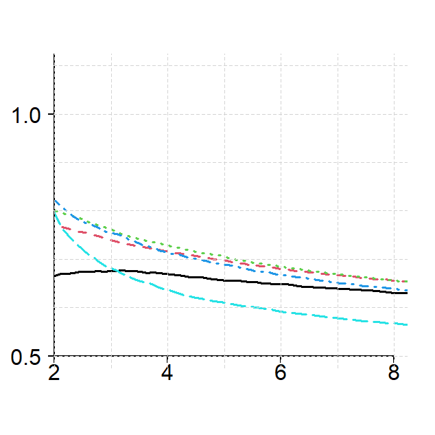
(d) $\hat{\chi}/\tilde{\chi}$

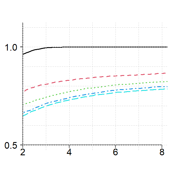
(e) $\hat{\chi}/\check{\chi}$

Figure 2: Homogeneous setup with known number of signals, $l=u\equiv m\in\{1,3,5,7,9\}$. The first row depicts the expected decision times in (6.6) and the second the relative efficiencies in (6.8). The first column refers to the proposed test, the second to the parallel SPRT, and the third to the synchronous test.

We consider first the homogeneous setup when the number of signals is a priori known to be equal to some $m\in\{1,\ldots,K-1\}$. We start with the first row in Figure 2, where the expected decision times of the three tests are presented.

• From Figure 2.(a) we can see that, for the proposed test, the expected decision time in a signal stream is the smallest when $m=9$, and it is overall decreasing in $m$, as expected in view of Remark 4.1.

• From Figure 2.(b) we can see that, for the parallel SPRT, the curves are horizontal translations of each other, moving to the right as $m$ increases. This is because we set $a=b$, in which case the expected decision time is the same in every stream and for every $m$, whereas the type-I familywise error rate decreases as $m$ increases.

• From Figure 2.(c) we can see that, for the synchronous test, the expected decision time is the largest when $m=K/2$, as expected in view of Remark 4.1. We also note that the expected decision time and the maximum familywise error rate coincide when $l=u$ is equal to $m$ and when it is equal to $K-m$, as expected by the symmetry of the setup.

We continue with the second row in Figure 2, where the relative efficiencies of the parallel SPRT and of the synchronous test against the proposed test are compared with their limits, which are given by (5.13) and (5.19), respectively. Specifically, in a homogeneous and symmetric setup with known number of signals, as the current one, the latter are in all streams equal to $1/2$ for the parallel SPRT and to $1$ for the synchronous test.

• From Figure 2.(d) we can see that, for the parallel SPRT, the convergence rate to $1/2$ is about the same for all values of $m$. Specifically, the relative efficiencies of the parallel SPRT compared with the proposed test are at most $82\%$ when $\alpha=0.01$ and at most $65\%$ when $\alpha=10^{-8}$.

• From Figure 2.(e) we can see that, for the synchronous test, the convergence to $1$ is very fast when $m=1$, but much slower when $m>1$. Indeed, when $m=1$, the synchronous test performs similarly to the proposed one, as expected by the second-order term in (4.19) and (4.21). On the other hand, when $m>1$, the relative efficiencies of the synchronous test compared with the proposed test are at most $78\%$ when $\alpha=0.01$ and at most $88\%$ when $\alpha=10^{-8}$. Therefore, when $m>1$, the proposed test performs significantly better than the synchronous test in this setup, even though the asymptotic relative efficiency is equal to 1 in every stream.

6.4.2 Lower and upper bounds on the number of signals

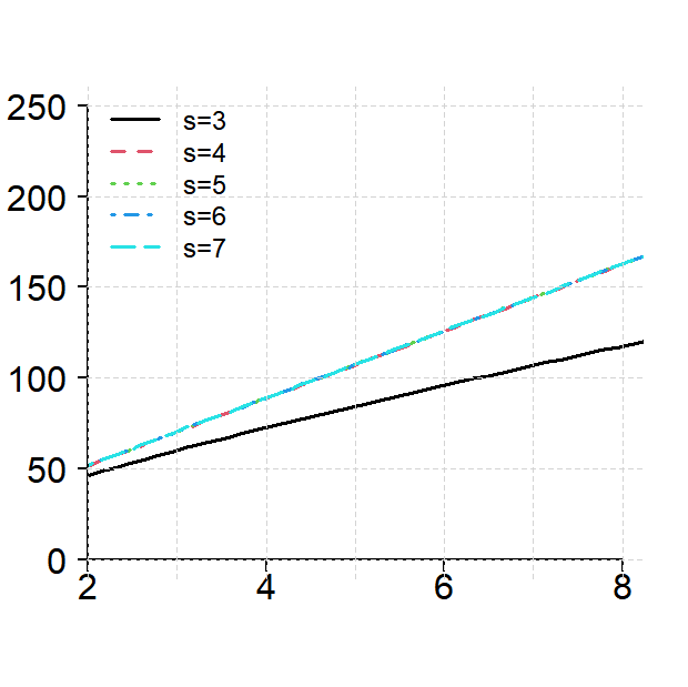
(a) $\hat{\chi}$

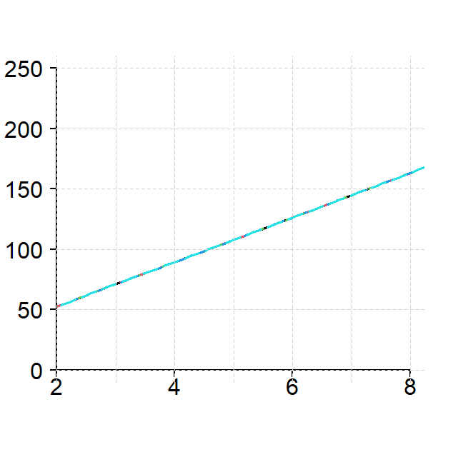
(b) $\tilde{\chi}$

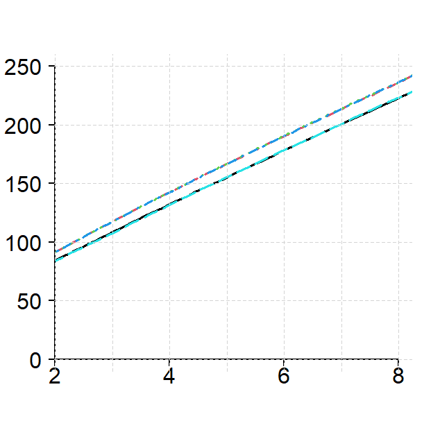
(c) $\check{\chi}$

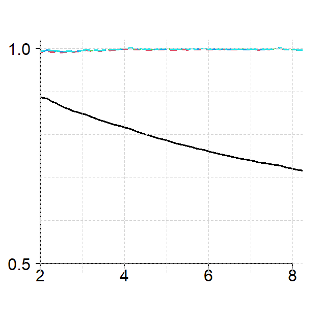
(d) $\hat{\chi}/\tilde{\chi}$

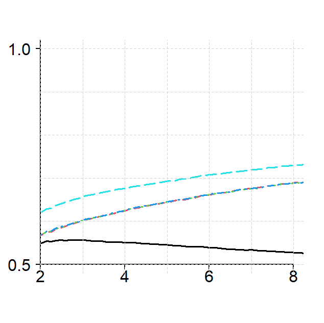
(e) $\hat{\chi}/\check{\chi}$

Figure 3: Homogeneous setup with $l=3$, $u=7$ and $|A|\equiv s\in\{3,4,5,6,7\}$. The first row depicts the expected decision times in (6.6) and the second the relative efficiencies in (6.8). The first column refers to the proposed test, the second to the parallel SPRT, and the third to the synchronous test.

We next consider the homogeneous setup when the number of signals is a priori known to be at least $l=3$ and at most $u=7$ and the true number of signals, $|A|$, is equal to some $s\in\{l,\ldots,u\}$. We start with the first row of Figure 3, where the expected decision times of the three tests are presented.

• From Figure 3.(a) we can see that the expected decision time of the proposed test in a signal stream is essentially the same for all values of $s$ with $s>l$, but much smaller when $s=l$, as expected by (5.5).

• From Figure 3.(b) we can see that the curves for the parallel SPRT coincide for all values of $s$. This is expected since its expected decision time in each stream does not depend on the true subset of signals when $a=b$.

• From Figure 3.(c) we can see that the curves for the synchronous test coincide when $s=l$ and $s=u=K-l$, and that they also coincide for all values of $s$ between $l$ and $u$.

We continue with the second row in Figure 3, where the relative efficiencies of the parallel SPRT and of the synchronous test against the proposed test are compared with their limits. From (5.13) and (5.19) it follows that the latter are equal, for both tests, to $1$ when $s>l$ and to $1/2$ when $s=l$.

From Figure 3.(d) and Figure 3.(e) we can see that the parallel SPRT performs substantially better than the synchronous test in all cases. Specifically, when $s>l$, its relative efficiencies are essentially equal to 1 even for large error probabilities, whereas those of the synchronous test never surpass $75\%$. When $s=l$, the relative efficiency of the parallel SPRT decreases to $1/2$ in a relatively slow rate, whereas that of the synchronous test is always below $60\%$

6.5 Results in the non-homogeneous setup

We next consider the non-homogeneous setup, (6.2), with $K=4$, $\mu=0.5$, $\phi=0.5$. In the case where the number of signals is not a priori known, we set $l=1$ and $u=3$. Unlike the homogeneous setup of the previous subsection, the expected decision times in (6.4) now do not depend only on the true number of signals, but also on the true subset of signals itself. We next focus on the following cases for the true subsets of signals:

• $A=\{1\}$, where $\mathcal{I}_{A}=\mathcal{J}_{A}=1/32$,

• $A=\{3\}$, where $\mathcal{I}_{A}=1/8$ and $\mathcal{J}_{A}=1/32$,

• $A=\{1,2\}$, where $\mathcal{I}_{A}=1/32$ and $\mathcal{J}_{A}=1/8$,

• $A=\{1,3\}$, where $\mathcal{I}_{A}=\mathcal{J}_{A}=1/32$.

As before, we consider two cases regarding the prior information. One where the number of signals is a priori known, i.e., $|A|=l=u$, and one where it is a priori known to be at least $l=1$ and at most $u=3$. The asymptotic relative efficiencies, given by (5.9) and (5.16) with $r=1$, are presented in Table 1 and 2.

	1	2	3	4
$\{1\}$	1/2	1/2	4/5	4/5
$\{3\}$	1/5	1/5	4/5	1/2
$\{1,2\}$	1/5	1/5	4/5	4/5
$\{1,3\}$	1/2	1/2	4/5	4/5

	1	2	3	4
$\{1\}$	1	1	2/5	2/5
$\{3\}$	1	1	1	5/8
$\{1,2\}$	1	1	1	1
$\{1,3\}$	1	1	2/5	2/5

Table 1: $\operatorname{ARE}^{\prime}_{k,A}(l,u)$ and $\operatorname{ARE}^{\prime\prime}_{k,A}(l,u)$ when $l=u=|A|$.

	1	2	3	4
$\{1\}$	1/2	1	1	1
$\{3\}$	1	1	4/5	1
$\{1,2\}$	1	1	1	1
$\{1,3\}$	1	1	1	1

	1	2	3	4
$\{1\}$	1/2	1	1/4	1/4
$\{3\}$	1	1	1/5	1/4
$\{1,2\}$	1	1	1/4	1/4
$\{1,3\}$	1	1	1/4	1/4

Table 2: $\operatorname{ARE}^{\prime}_{k,A}(l,u)$ and $\operatorname{ARE}^{\prime\prime}_{k,A}(l,u)$ when $l=1,u=3$.

We present the plots for the case of $l=u$ in Table 3 and for the case of $l=1$, $u=3$ in Table 4. In each of these two tables of plots, each column corresponds to one of the four cases for $A$ in (i)-(iv). The first row depicts the expected decision times of the parallel SPRT in each of the four streams. The second row depicts the corresponding plots for the proposed test and the synchronous test. The third (resp. fourth) row depicts the relative efficiencies of the parallel SPRT (resp. synchronous test) against the proposed test in each of the four streams. The corresponding limiting values from Tables 1 and 2 are marked on the vertical axis. In all plots, the horizontal axis represents the absolute value of the base-10 logarithm of the maximum type-I (resp. -II) familywise error rate if that stream is a signal (resp. noise).

From the third and the fourth row in each table of plots we can see that in all cases the relative efficiencies converge to their limiting values very quickly. Thus, in this setup, the latter provide a very accurate approximation of the actual relative efficiencies.

	(i)	(ii)	(iii)	(iv)
$\tilde{\chi}$
$\hat{\chi}$, $\check{\chi}$
$\hat{\chi}/\tilde{\chi}$
$\hat{\chi}/\check{\chi}$

Table 3: Non-homogeneous setup with known number of signals. Each column corresponds to a case for the true subset of signals. The horizontal axis represents the absolute value of the base-10 logarithm of the maximum familywise type-I or -II error rate, depending on whether the stream is a signal or a noise. The vertical axis in the first (resp. second) row represents the expected decision times of the parallel SPRT, $\tilde{\chi}$ (resp. the proposed test, $\hat{\chi}$, and the synchronous test, $\check{\chi}$). The vertical axis in the third (resp. fourth) row represents the relative efficiencies of $\tilde{\chi}$ (resp. $\check{\chi}$) against $\hat{\chi}$. The asymptotic relative efficiencies in Table 1 are marked on the vertical axis in the third and fourth rows.

	(i)	(ii)	(iii)	(iv)
$\tilde{\chi}$
$\hat{\chi}$, $\check{\chi}$
$\hat{\chi}/\tilde{\chi}$
$\hat{\chi}/\check{\chi}$

Table 4: Non-homogeneous setup with lower bound $l=1$ and upper bound $u=3$ on the number signals. The meaning of each column, each row and each axis is the same as Table 3. There is only one plot in the first row because the corresponding plots for the parallel SPRT are exactly the same in all cases regarding the true subset of signals. The limits for the relative efficiencies, which are marked on the vertical axis in the third and fourth rows, are give by Table 2.

7 Generalization to parametric composite hypotheses

In this section we extend the methodology and results of the previous sections to general, parametric composite hypotheses, following the adaptive likelihood ratio approach in Robbins and Siegmund (1974); Pavlov (1991) and (Song and Fellouris, 2019, Section 6) (see, also, (Tartakovsky et al., 2014, Chapter 5)).

Thus, for each $k\in[K]$, we assume that the distribution of $X_{k}$ is specified up to an unknown parameter that belongs to a subset $\Theta_{k}$ of some Euclidean space, and denote it by $\mathrm{P}_{k,\theta}$ when the value of this parameter is $\theta$. In this context, the hypotheses in (2.1) are of the form

$$\mathcal{P}_{k}^{i}=\{\mathrm{P}_{k,\theta},\,\theta\in\Theta^{i}_{k}\},\quad i\in\{0,1\},$$

where $\Theta_{k}^{0}$ and $\Theta_{k}^{1}$ are two disjoint subsets of $\Theta_{k}$, and the goal is to minimize the expected decision time simultaneously in every stream and for every possible value of the unknown parameter, while controlling the worst-case type-I and type-II familywise error rates. To be specific, we denote by ${\boldsymbol{\Theta}}$ the global parameter space, i.e.,

$${\boldsymbol{\Theta}}\equiv\Theta_{1}\times\cdots\times\Theta_{K},$$

and for any $A\subseteq[K]$, denote by ${\boldsymbol{\Theta}}_{A}$ its subset that is consistent with the subset of signals being $A$, i.e.,

$${\boldsymbol{\Theta}}_{A}\equiv\left\{(\theta_{1},\ldots,\theta_{K})\in{\boldsymbol{\Theta}}:\quad\theta_{i}\in\Theta_{i}^{1},\quad\theta_{j}\in\Theta_{j}^{0},\quad i\in A,\quad j\notin A\right\}.$$

For any ${\boldsymbol{\theta}}=(\theta_{1},\ldots,\theta_{K})\in\Theta_{A}$ we denote by $\mathrm{P}_{A,{\boldsymbol{\theta}}}$ the joint distribution of all streams when the subset of signals is $A$ and the parameter is ${\boldsymbol{\theta}}$, by $\mathrm{E}_{A,{\boldsymbol{\theta}}}$ the corresponding expectation, and we note that by the assumption of independence across streams we have

$$\mathrm{P}_{A,{\boldsymbol{\theta}}}=\mathrm{P}_{1,\theta_{1}}\otimes\cdots\otimes\mathrm{P}_{K,\theta_{K}}.$$

Then, for any $\alpha,\beta\in(0,1)$ and $\Pi\subseteq 2^{[K]}$, the class of admissible tests takes the following form:

$$\Delta^{*}(\alpha,\beta,\Pi)\equiv\bigg{\{}\chi\in\Delta:\,\sup_{{\boldsymbol{\theta}}\in{\boldsymbol{\Theta}}_{A}}\mathrm{P}_{A,{\boldsymbol{\theta}}}(\mathbf{D}\backslash A\neq\emptyset) \leq\alpha$$

$$\text{and}\quad\sup_{{\boldsymbol{\theta}}\in{\boldsymbol{\Theta}}_{A}}\mathrm{P}_{A,{\boldsymbol{\theta}}}(A\backslash\mathbf{D}\neq\emptyset) \leq\beta,\quad\forall\,A\in\Pi\bigg{\}},$$

and the goal is to achieve

$$\inf\big{\{}\mathrm{E}_{A,{\boldsymbol{\theta}}}[T_{k}]:\chi\in\Delta^{*}(\alpha,\beta,\Pi)\big{\}}$$

simultaneously for every $k\in[K]$, $A\in\Pi$, ${\boldsymbol{\theta}}\in{\boldsymbol{\Theta}}_{A}$, as $\alpha,\beta\to 0$.

7.1 The sequential tests

We next generalize the testing procedures in Section 3 to the composite testing setup. To do this, for each $k\in[K]$, $\theta\in\Theta_{k}$, and $n\in\mathbb{N}$, we assume that $\mathrm{P}_{k,\theta}$ is dominated by a $\sigma$-finite measure $\nu_{k}$ when both measures are restricted to $\mathcal{F}_{k}(n)$, and we denote by $\ell_{k}(n,\theta)$ the corresponding log-likelihood function, i.e.,

$$\ell_{k}(n,\theta)\equiv\log\frac{d\mathrm{P}_{k,\theta}}{d\nu_{k}}(\mathcal{F}_{k}(n)),\quad\theta\in\Theta_{k},$$

and by $(\Delta\ell)_{k}(n,\theta)$ its increment at time $n$, i.e.,

$$(\Delta\ell)_{k}(n,\theta)\equiv\ell_{k}\left(n,\theta\right)-\ell_{k}\left(n-1,\theta\right),\quad\text{where}\quad\ell_{k}(0)\equiv 0.$$

We assume that, for each $k\in[K]$ and $n\in\mathbb{N}$, we have an $\mathcal{F}(n)$-measurable estimator of $\theta_{k}$, $\hat{\theta}_{k}(n)$, and we define the adaptive log-likelihood in stream $k$ at time $n$ as

$$\ell^{*}_{k}(n)\equiv\ell^{*}_{k}(n-1)+(\Delta\ell)_{k}\big{(}n,\hat{\theta}_{k}(n-1)\big{)},\quad\text{where}\quad\ell^{*}_{k}(0)\equiv 0,$$

with $\hat{\theta}_{k}(0)$ being an arbitrary deterministic value in $\Theta_{k}$. The tests we propose in the composite testing setup are essentially the same as the ones in Section 3 with the difference that the LLR statistic in stream $k$ at time $n$, $\lambda_{k}(n)$, is now replaced by the following adaptive log-likelihood ratio:

$$\lambda^{*}_{k}(n)=\begin{cases}\begin{aligned} &\ell^{*}_{k}(n)-\ell_{k}^{0}(n),&&\text{if }\ell_{k}^{0}(n)<\min\left\{\ell_{k}^{1}(n),\ell^{*}_{k}(n)\right\}\\ &\ell_{k}^{1}(n)-\ell^{*}_{k}(n),&&\text{if }\ell_{k}^{1}(n)<\min\left\{\ell_{k}^{0}(n),\ell^{*}_{k}(n)\right\}\\ &0,&&\text{otherwise},\end{aligned}\end{cases}$$ (7.1)

where, for each $i\in\{0,1\}$, $\ell_{k}^{i}(n)$ is the maximum log-likelihood under $\Theta_{k}^{i}$, i.e.,

$$\ell_{k}^{i}(n)\equiv\sup\left\{\ell_{k}(n,\theta):\theta\in\Theta_{k}^{i}\right\},\quad i\in\{0,1\}.$$ (7.2)

7.1.1 The decentralized test

The decentralized test is defined as in (3.1)-(3.2) with $\lambda_{k}(n)$ replaced by $\lambda^{*}_{k}(n)$, as long as $\hat{\theta}_{k}(n)$ is an estimator of the unknown parameter in stream $k$ that depends only on the observations from that stream up to time $n$, i.e., $\hat{\theta}_{k}(n)$ is $\mathcal{F}_{k}(n)$-measurable for every $k\in[K]$ and $n\in\mathbb{N}$.

7.1.2 The proposed test

The proposed test is given by (3.3), where $\hat{T}_{k,1}$ and $\hat{T}_{k,2}$ now take the following form:

• When $l=u\equiv m$,

  $$\hat{T}_{k,1} \equiv\inf\left\{n\in\mathbb{N}:\lambda^{*}_{k}(n)>\max\big{\{}\lambda^{*}_{(m+1)}(n)+c,\,0\big{\}},\;\lambda^{*}_{(m+1)}(n)<0\right\},$$

  $$\hat{T}_{k,2} \equiv\inf\left\{n\in\mathbb{N}:\lambda^{*}_{k}(n)<\min\big{\{}\lambda^{*}_{(m)}(n)-d,\,0\big{\}},\;\lambda^{*}_{(m)}(n)>0\right\},$$

  where $c,d>0$ are thresholds to be determined.
  

• When $l<u$,

  $$\hat{T}_{k,1}\equiv \inf\left\{n\in\mathbb{N}:\lambda^{*}_{k}(n)>a\right\}\bigwedge$$

  $$\inf\left\{n\in\mathbb{N}:\lambda^{*}_{k}(n)>\max\big{\{}\lambda^{*}_{(l+1)}(n)+c,\,0\big{\}},\;\lambda^{*}_{(l+1)}(n)<0\right\},$$

  $$\hat{T}_{k,2}\equiv \inf\left\{n\in\mathbb{N}:\lambda^{*}_{k}(n)<-b\right\}\bigwedge$$ (7.3)

  $$\inf\left\{n\in\mathbb{N}:\lambda^{*}_{k}(n)<\min\big{\{}\lambda^{*}_{(u)}(n)-d,\,0\big{\}},\;\lambda^{*}_{(u)}(n)>0\right\},$$

  where $a,b,c,d>0$ are thresholds to be determined.

7.1.3 The synchronous test

The synchronous test takes the following form:

• When $l=u\equiv m$,

  $$\check{T}\equiv\inf\left\{n\in\mathbb{N}:\lambda^{*}_{(m)}(n)-\lambda^{*}_{(m+1)}(n)>c\vee d,\;\lambda^{*}_{(m+1)}(n)<0<\lambda^{*}_{(m)}(n)\right\},$$

  and $\check{\mathbf{D}}$ is the subset of the $m$ streams with the largest values of $\lambda^{*}_{k}(\check{T})$, $k\in[K]$.

• When $l<u$,

  $$\check{T} \equiv\tau_{1}\wedge\tau_{2}\wedge\tau_{3},\quad\text{where}$$

  $$\tau_{1} \equiv\inf\left\{n\in\mathbb{N}:\lambda^{*}_{(l+1)}(n)<\min\big{\{}-b,-c+\lambda^{*}_{(l)}(n)\big{\}},\;\lambda^{*}_{(l)}(n)>0\right\},$$

  $$\tau_{2} \equiv\inf\left\{n\in\mathbb{N}:\lambda^{*}_{k}(n)\notin(-b,a)\;\forall\,k\in[K],\text{ and }l\leq p^{*}(n)\leq u\right\},$$

  $$\tau_{3} \equiv\inf\left\{n\in\mathbb{N}:\lambda^{*}_{(u)}(n)>\max\big{\{}a,\,d+\lambda^{*}_{(u+1)}(n)\big{\}},\;\lambda^{*}_{(u+1)}(n)<0\right\},$$

  and $\check{\mathbf{D}}$ is the subset of the $\left(p^{*}(\check{T})\vee l\right)\wedge u$ streams with the largest values of $\lambda^{*}_{k}(\check{T})$, $k\in[K]$, where $p^{*}(n)\equiv\left|\{k\in[K]:\lambda^{*}_{k}(n)>0\}\right|$.

7.2 Distributional assumptions

We next state the distributional assumptions that we need to make in order to generalize the asymptotic optimality theory of Section 5.

First of all, we assume that for every $k\in[K]$ and $\theta,u\in\Theta_{k}$ there exists a positive number $I_{k}(\theta,u)$ such that

$$\mathrm{P}_{k,\theta}\left(\limsup_{n\to\infty}\frac{\ell_{k}(n,\theta)-\ell_{k}(n,u)}{n}\leq I_{k}(\theta,u)\right)=1.$$ (7.4)

Second, we assume that the null and alternative hypotheses in each stream are separated, in the sense that, for each $k\in[K]$,

$$\begin{split}I_{k}(\theta)&\equiv\inf_{u\in\Theta_{k}^{0}}I_{k}(\theta,u)>0,\quad\forall\,\theta\in\Theta_{k}^{1},\\ J_{k}(\theta)&\equiv\inf_{u\in\Theta_{k}^{1}}I_{k}(\theta,u)>0,\quad\,\forall\,\theta\in\Theta_{k}^{0}.\end{split}$$ (7.5)

Finally, we assume that for each $k\in[K]$ and $\epsilon>0$,

$$\begin{gathered}\sum_{n=1}^{\infty}\mathrm{P}_{k,\theta}\left(\frac{\ell^{*}_{k}(n)-\ell_{k}^{0}(n)}{n}\leq I_{k}(\theta)-\epsilon\right)<\infty,\quad\forall\,\theta\in\Theta_{k}^{1},\\ \sum_{n=1}^{\infty}\mathrm{P}_{k,\theta}\left(\frac{\ell^{*}_{k}(n)-\ell_{k}^{1}(n)}{n}\leq J_{k}(\theta)-\epsilon\right)<\infty,\quad\forall\,\theta\in\Theta_{k}^{0}.\end{gathered}$$ (7.6)

Remark 7.1.

Assumptions (7.4)-(7.6) are satisfied when, for example, $X_{k}$ is an i.i.d. sequence whose distribution belongs to some multi-parameter exponential family, both the null and the alternative parameter spaces, $\Theta_{0}^{k}$ and $\Theta_{1}^{k}$, are compact, and $\hat{\theta}_{k}(n)$ is the maximal likelihood estimator based on the observations from stream $k$ up to time $n$, i.e.,

$$\hat{\theta}_{k}(n)\equiv\operatorname{argmax}\left\{\ell_{k}(n,\theta_{k}):\theta_{k}\in\Theta_{k}^{0}\cup\Theta_{k}^{1}\right\}$$

(see, e.g., (Song and Fellouris, 2019, Appendix E)).

7.3 Asymptotic optimality

We are now ready to generalize the asymptotic optimality theorems of Section 5 to the case of general composite hypotheses. To state these results, for any $A\subseteq[K]$ and ${\boldsymbol{\theta}}=(\theta_{1},\ldots,\theta_{K})\in{\boldsymbol{\Theta}}_{A}$ we set

$$\mathcal{I}_{A}({\boldsymbol{\theta}})\equiv\min_{i\in A}I_{i}(\theta_{i})\qquad\text{ and }\qquad\mathcal{J}_{A}({\boldsymbol{\theta}})\equiv\min_{j\notin A}J_{j}(\theta_{j}).$$

Theorem 7.1.

Let $l,u$ satisfy (2.3). Suppose that the thresholds of $\hat{\chi}$ are selected so that $\hat{\chi}\in\Delta^{*}(\alpha,\beta,\Pi_{l,u})$ for any $\alpha,\beta\in(0,1)$ and also (5.4) holds, e.g., according to (4.9) when $l=u$ and (4.10) when $l<u$.

If conditions (7.4)-(7.6) hold for every $k\in[K]$, then, as $\alpha,\beta\to 0$,

$$\mathrm{E}_{A,{\boldsymbol{\theta}}}[\hat{T}_{i}] \sim\inf\big{\{}\mathrm{E}_{A,{\boldsymbol{\theta}}}[T_{i}]:\chi\in\Delta^{*}(\alpha,\beta,\Pi_{l,u})\big{\}}$$ (7.7)

$$\sim\frac{|\log\alpha|}{I_{i}(\theta_{i})+\mathcal{J}_{A}({\boldsymbol{\theta}})\cdot\mathbf{1}\left\{|A|=\ell\right\}}$$

$$\mathrm{E}_{A,{\boldsymbol{\theta}}}[\hat{T}_{j}] \sim\inf\big{\{}\mathrm{E}_{A,{\boldsymbol{\theta}}}[T_{j}]:\chi\in\Delta^{*}(\alpha,\beta,\Pi_{l,u})\big{\}}$$ (7.8)

$$\sim\frac{|\log\beta|}{J_{j}(\theta_{j})+\mathcal{I}_{A}({\boldsymbol{\theta}})\cdot\mathbf{1}\left\{|A|=u\right\}}$$

simultaneously for every $i\in A$, $j\notin A$, $A\in\Pi_{l,u}$, ${\boldsymbol{\theta}}\in{\boldsymbol{\Theta}}_{A}$.

Proof.

Appendix D.
∎

Theorem 7.2.

Let $\Pi$ satisfy (2.2). Suppose that the thresholds of $\tilde{\chi}$ are selected so that $\tilde{\chi}\in\Delta^{*}(\alpha,\beta,\Pi)$ for any $\alpha,\beta\in(0,1)$ and also (5.7) holds, e.g., according to (4.8).

If conditions (7.4)-(7.6) hold for every $k\in[K]$, then, as $\alpha,\beta\to 0$,

$$\begin{split}\mathrm{E}_{A,{\boldsymbol{\theta}}}[\tilde{T}_{i}]&\sim\inf\left\{\mathrm{E}_{A,{\boldsymbol{\theta}}}[T_{i}]:\chi\in\Delta^{\prime}\cap\Delta^{*}(\alpha,\beta,\Pi)\right\}\sim\frac{|\log\alpha|}{I_{i}(\theta_{i})}\\ \mathrm{E}_{A,{\boldsymbol{\theta}}}[\tilde{T}_{j}]&\sim\inf\big{\{}\mathrm{E}_{A,{\boldsymbol{\theta}}}[T_{j}]:\chi\in\Delta^{\prime}\cap\Delta^{*}(\alpha,\beta,\Pi)\big{\}}\sim\frac{|\log\beta|}{J_{j}(\theta_{j})}\end{split}$$

simultaneously for every $i\in A$, $j\notin A$, $A\in\Pi$, ${\boldsymbol{\theta}}\in{\boldsymbol{\Theta}}_{A}$.

Proof.

Appendix D.
∎

Theorem 7.3.

Let $l,u$ satisfy (2.3). Suppose that the thresholds of $\check{\chi}$ are selected so that $\check{\chi}\in\Delta^{*}(\alpha,\beta,\Pi_{l,u})$ for any $\alpha,\beta\in(0,1)$ and also (5.4) holds, e.g., according to (4.9) when $l=u$ and (4.10) when $l<u$.

If conditions (7.4)-(7.6) hold for every $k\in[K]$, then, as $\alpha,\beta\to 0$,

$$\begin{split}\mathrm{E}_{A,{\boldsymbol{\theta}}}[\check{T}]&\sim\inf\big{\{}\mathrm{E}_{A,{\boldsymbol{\theta}}}[T_{1}]:\chi\in\Delta^{\prime\prime}\cap\Delta^{*}(\alpha,\beta,\Pi_{l,u})\big{\}}\\ &\sim\max\left\{\frac{|\log\alpha|}{\mathcal{I}_{A}({\boldsymbol{\theta}})+\mathcal{J}_{A}({\boldsymbol{\theta}})\cdot\mathbf{1}\{|A|=l\}},\;\frac{|\log\beta|}{\mathcal{J}_{A}({\boldsymbol{\theta}})+\mathcal{I}_{A}({\boldsymbol{\theta}})\cdot\mathbf{1}\{|A|=u\}}\right\}\end{split}$$

simultaneously for every $A\in\Pi_{l,u}$, ${\boldsymbol{\theta}}\in{\boldsymbol{\Theta}}_{A}$.

Proof.

Appendix D.
∎

8 Generalization to other global error metrics

In this section, we discuss the extension of the asymptotic optimality theory of Section 5 to various error metrics beyond the classical familywise error rates. For this, we follow the approach in He and Bartroff (2021), where the asymptotic optimality theory for synchronous tests in Song and Fellouris (2017) was extended to general error metrics.

For simplicity, we focus on the case of simple hypotheses and in the place of the familywise error rates, $\text{FWE}_{A}^{1}(\chi)$ and $\text{FWE}_{A}^{2}(\chi)$, of a test $\chi\in\Delta$, we consider the type-I and type-II versions of a generic error metric

$$\text{GEM}_{A}^{1}(\chi)\qquad\text{ and }\qquad\text{GEM}_{A}^{2}(\chi).$$

Then, $\hat{\chi}$, $\tilde{\chi}$, $\check{\chi}$ can be designed to control these error metrics and preserve their asymptotic optimality properties as long as there exist $C_{1},C_{2}>0$ so that, for both $i\in\{1,2\}$ and every $A\in\Pi$,

$$\text{GEM}_{A}^{i}(\chi) \leq C_{1}\cdot\text{FWE}_{A}^{i}(\chi)\quad\text{for all}\quad\chi\in\{\hat{\chi},\tilde{\chi},\check{\chi}\},$$ (8.1)

$$\text{and}\quad\text{GEM}_{A}^{i}(\chi) \geq C_{2}\cdot\text{FWE}_{A}^{i}(\chi)\quad\text{for all}\quad\chi\in\Delta.$$ (8.2)

To see this, for any $\alpha,\beta\in(0,1)$ and $\Pi$ we set

$$\Delta^{\text{GEM}}(\alpha,\beta,\Pi)\equiv\bigg{\{}\chi\in\Delta:\;\text{GEM}_{A}^{1}(\chi)\leq\alpha\;\text{ and }\;\text{GEM}_{A}^{2}(\chi)\leq\beta,\;\forall\;A\in\Pi\bigg{\}}.$$

Then, by (8.1) we have

$$\chi\in\{\hat{\chi},\tilde{\chi},\check{\chi}\}\quad\text{and}\quad\chi\in\Delta(\alpha/C_{1},\beta/C_{1},\Pi)\quad\Rightarrow\quad\chi\in\Delta^{\text{GEM}}(\alpha,\beta,\Pi),$$

whereas (8.2) implies that, for every $A\in\Pi$ and $k\in[K]$, as $\alpha,\beta\to 0$,

$$\begin{split}\inf\left\{\mathrm{E}_{A}[T_{k}]:\chi\in\Delta^{\text{GEM}}(\alpha,\beta,\Pi)\right\}&\geq\mathcal{L}_{k,A}(\alpha/C_{2},\beta/C_{2},\Pi)\sim\mathcal{L}_{k,A}(\alpha,\beta,\Pi)\\ \inf\left\{\mathrm{E}_{A}[T_{k}]:\chi\in\Delta^{\prime}\cap\Delta^{\text{GEM}}(\alpha,\beta,\Pi)\right\}&\geq\mathcal{L}^{\prime}_{k,A}(\alpha/C_{2},\beta/C_{2},\Pi)\sim\mathcal{L}^{\prime}_{k,A}(\alpha,\beta,\Pi)\\ \inf\left\{\mathrm{E}_{A}[T_{1}]:\chi\in\Delta^{\prime\prime}\cap\Delta^{\text{GEM}}(\alpha,\beta,\Pi)\right\}&\geq\mathcal{L}^{\prime\prime}_{A}(\alpha/C_{2},\beta/C_{2},\Pi)\sim\mathcal{L}^{\prime\prime}_{A}(\alpha,\beta,\Pi).\end{split}$$

We next provide some concrete examples of error metrics that satisfy the above conditions when $\Pi$ is of the form $\Pi_{l,u}$.

• Per-comparison error rates (PCE): the expected proportion of type-I or type-II errors among all streams:

  $$\text{PCE}_{A}^{1}(\chi)\equiv\frac{\mathrm{E}_{A}[|\mathbf{D}\backslash A|]}{K}\qquad\text{and}\qquad\text{PCE}_{A}^{2}(\chi)\equiv\frac{\mathrm{E}_{A}[|A\backslash\mathbf{D}|]}{K}.$$

• False discovery rate (FDR) and false non-discovery rate: the expected proportion of type-I errors among all streams identified as signals and the expected proportion of type-II errors among all streams identified as noises:

  $$\text{FDR}_{A}^{1}(\chi)\equiv\mathrm{E}_{A}\left[\frac{|\mathbf{D}\backslash A|}{|\mathbf{D}|}\right]\qquad\text{and}\qquad\text{FDR}_{A}^{2}(\chi)\equiv\mathrm{E}_{A}\left[\frac{|A\backslash\mathbf{D}|}{K-|\mathbf{D}|}\right],$$

  with the convention that $0/0=0$.

• Positive false discovery rate (pFDR) and positive false non-discovery rate: the expected proportion of type-I (resp. -II) errors among all streams identified as signals (resp. noises) given that there are streams identified as signals (resp. noises):

  $$\text{pFDR}_{A}^{1}(\chi) \equiv\mathrm{E}_{A}\left[\left.\frac{|\mathbf{D}\backslash A|}{|\mathbf{D}|}\;\right|\;|\mathbf{D}|\geq 1\right]$$

  $$\text{pFDR}_{A}^{2}(\chi) \equiv\mathrm{E}_{A}\left[\left.\frac{|A\backslash\mathbf{D}|}{K-|\mathbf{D}|}\;\right|\;K-|\mathbf{D}|\geq 1\right].$$

Indeed, by He and Bartroff (2021) it follows that the inequalities (8.1)-(8.2) hold when $\Pi=\Pi_{l,u}$ and

• $\text{GEM}=\text{PCE}$, with $C_{1}=(u\vee(K-l))/K$, $C_{2}=1/K$.

• $\text{GEM}=\text{FDR}$, with $C_{1}=1$, $C_{2}=1/K$.

The next Proposition deals with the error metric in (iii).

Proposition 8.1.

Let $\Pi=\Pi_{l,u}$, where $0<l\leq u<K$, and suppose that $\text{FWE}_{A}^{i}(\chi)\leq 1/2$, where $i\in\{0,1\}$ and $\chi\in\{\hat{\chi},\tilde{\chi},\check{\chi}\}$. If $\text{GEM}=\text{pFDR}$, then the inequalities (8.1)-(8.2) hold with $C_{1}=2$, $C_{2}=1/K$.

Proof.

See Appendix E. ∎

9 Conclusion and open problems

In this work we consider the problem of simultaneously testing the marginal distributions of multiple, sequentially monitored data streams. We introduce a general formulation in which the decisions for the various testing problems can be made at different times, using data from all streams, and all streams can be monitored until all decisions have been made. Assuming a priori bounds on the number of signals, we propose a novel sequential multiple testing procedure that takes advantage of the flexibility of this formulation. Under general distributional assumptions and in the case of general parametric composite hypotheses, we show that the proposed procedure minimizes the expected decision time, simultaneously for every data stream and for every signal configuration, asymptotically as the target error rates go to zero. In this asymptotic regime, we also evaluate the factor by which the expected decision time in every stream increases when one is limited to decentralized procedures, where only local data can be used for each testing problem, or synchronous procedures, where all decisions must be made at the same time.

There are various directions for further study. First of all, it is interesting to develop an analogous asymptotic optimality theory when sampling from a data stream must be terminated once the decision for the corresponding testing problem has been made, and data from all streams can be utilized for each testing problem. This setup, which is considered, for example, in Bartroff and Song (2014), is more restrictive than the one we consider in the present paper, where all streams can be monitored until all decisions have been made. However, it is more flexible than a decentralized setup, where it is possible to use only local data for each testing problem. The results of the present paper indicate that this additional flexibility does not provide any gains, as far as it concerns first-order asymptotic optimality, when there is no prior information regarding the subset of signals. An asymptotic optimality theory in the case where non-trivial prior information is available is an open problem.

Second, it is interesting to extend the formulation of the present paper to the case where it is possible to observe only a subset of data streams at each time instant, which is determined by the practitioner based on the already collected observations. Such sampling constraints have been considered in various works, such as Cohen and Zhao (2015); Huang et al. (2018); Hemo et al. (2020); Tsopelakos and Fellouris (2022); Prabhu et al. (2022), but in all of them a common decision time is assumed.

Finally, another direction of interest is to consider error metrics that are not bounded by the familywise error rates up to multiplicative constants and, as a result, the results of Section 8 do not apply. This is the case, for example, for the generalized familywise error rates Lehmann and Romano (2005) or the generalized false discovery/non-discovery rate Sarkar (2007). The former has been considered in the case of synchronous procedures in Song and Fellouris (2019). An asymptotic optimality theory with such error metrics in the general family of sequential multiple testing procedures of the present work is an open problem.

Appendix A

In this Appendix, we state and prove three supporting lemmas. The first two are used in the proof of the asymptotic upper bounds in Propositions 4.2 and 4.3, whereas the third is used in the proof of the asymptotic lower bound in Lemma 5.1.

Lemma A.1.

Let $\xi_{l}\equiv\{\xi_{l}(n),\,n\in\mathbb{N}\}$, $l\in[L]$ be $L\in\mathbb{N}$ stochastic processes on some probability space $(\Omega,\mathcal{F},\mathrm{P})$. For any $\mathbf{a}=\{a_{1},\ldots,a_{L}\}$ where $a_{l}\geq 0$ for every $l\in[L]$, set

$$\nu(\mathbf{a})\equiv\inf\{n\in\mathbb{N}:\,\xi_{l}(n)\geq a_{l}\text{ for every }l\in[L]\}.$$

If for each $l\in[L]$ there exists $\mu_{l}>0$ so that

$$\forall\;\epsilon>0\quad\sum_{n=1}^{\infty}\mathrm{P}\left(\frac{1}{n}\xi_{l}(n)\leq\mu_{l}-\epsilon\right)<\infty,$$

then, as $\min_{l\in[L]}a_{l}\to\infty$,

$$\mathrm{E}[\nu(\mathbf{a})]\lesssim\max_{l\in[L]}\left\{\frac{a_{l}}{\mu_{l}}\right\},$$

where $\mathrm{E}$ is the expectation under $\mathrm{P}$.

Proof.

See (Song and Fellouris, 2019, Lemma F.2).
∎

Lemma A.2.

Let $\xi_{l},\;l\in[L]$ and $\nu(\mathbf{a})$ be defined the same as in Lemma A.1. If, for each $l\in[L]$, $\{\xi_{l}(n)-\xi_{l}(n-1),\;n\in\mathbb{N}\}$ where $\xi_{l}(0)=0$ are i.i.d.,

$$\mathrm{E}[\xi_{l}(1)]=\mu_{l}>0\quad\text{and}\quad\operatorname{Var}(\xi_{l}(1))<\infty,$$

then, as $\min_{l\in[L]}a_{l}\to\infty$,

$$\mathrm{E}[\nu(\mathbf{a})]\leq\max_{l\in[L]}\left\{\frac{a_{l}}{\mu_{l}}\right\}+O\left(\sum_{l\in[L]}\sqrt{\frac{a_{l}}{\mu_{l}}}\right)\leq\max_{l\in[L]}\left\{\frac{a_{l}}{\mu_{l}}\right\}+O\left(L\sqrt{\max_{l\in[L]}a_{l}}\right).$$

Proof.

See (Song and Fellouris, 2017, Lemma A.2.).
∎

Lemma A.3.

Let $\xi\equiv\{\xi(n),\,n\in\mathbb{N}\}$ be a stochastic process on some probability space $(\Omega,\mathcal{F},\mathrm{P})$. Suppose that

$$\mathrm{P}\left(\limsup_{n\to\infty}\frac{\xi(n)}{n}\leq\mu\right)=1,$$

then for any $\epsilon>0$ we have

$$\lim_{m\to\infty}\mathrm{P}\left(\frac{1}{m}\max_{1\leq n\leq m}\xi(n)>(1+\epsilon)\mu\right)=0.$$

Proof.

Fix $\epsilon>0$ and $1\leq N<m$. Denote

$$\mathrm{P}_{m,N}(\epsilon) \equiv\mathrm{P}\left(\frac{1}{m}\max_{1\leq n\leq N}\xi(n)>(1+\epsilon)\mu\right)$$

$$U_{N}(\epsilon) \equiv\left\{\sup_{n>N}\frac{\xi(n)}{n}>(1+\epsilon)\mu\right\}.$$

By the union bound, we have

$$\mathrm{P}\left(\frac{1}{m}\max_{1\leq n\leq m}\xi(n)>(1+\epsilon)\mu\right) \leq\mathrm{P}_{m,N}(\epsilon)+\mathrm{P}\left(\frac{1}{m}\max_{N<n\leq m}\xi(n)>(1+\epsilon)\mu\right)$$

$$\leq\mathrm{P}_{m,N}(\epsilon)+\mathrm{P}\left(\max_{N<n\leq m}\frac{\xi(n)}{n}>(1+\epsilon)\mu\right)$$

$$\leq\mathrm{P}_{m,N}(\epsilon)+\mathrm{P}(U_{N}(\epsilon)).$$

Since $\xi(n)$ is finite almost surely for every $n\in\mathbb{N}$, we have $\mathrm{P}_{m,N}(\epsilon)\to 0$ as $m\to\infty$ and, consequently,

$$\limsup_{m\to\infty}\mathrm{P}\left(\frac{1}{m}\max_{1\leq n\leq m}\xi(n)>(1+\epsilon)\mu\right)\leq\mathrm{P}(U_{N}(\epsilon)).$$

Finally, by the assumption of the Lemma it follows that, as $N\to\infty$, we have

$$\limsup_{N\to\infty}\mathrm{P}(U_{N}(\epsilon)) \leq\mathrm{P}\left(\inf_{N\geq 1}\sup_{n>N}\frac{\xi(n)}{n}\geq(1+\epsilon)\mu\right)$$

$$\leq\mathrm{P}\left(\limsup_{n}\frac{\xi(n)}{n}>\mu\right)=0.$$

∎

Appendix B

In this Appendix we prove Propositions 4.1, 4.2, and 4.3. For any $A,C\subseteq[K]$ and $n\in\mathbb{N}$, we denote by $\lambda_{A,C}(n)$ the log-likelihood ratio of $\mathrm{P}_{A}$ versus $\mathrm{P}_{C}$ when both measures are restricted to $\mathcal{F}(n)$, i.e.,

$$\lambda_{A,C}(n)\equiv\log\frac{d\mathrm{P}_{A}}{d\mathrm{P}_{C}}(\mathcal{F}(n))=\sum_{k\in A\backslash C}\lambda_{k}(n)-\sum_{k\in C\backslash A}\lambda_{k}(n),$$ (B.1)

where the equality follows by (2.4). We set $\lambda_{A,C}\equiv\{\lambda_{A,C}(n),n\in\mathbb{N}\}$. Moreover, if $\mathrm{E}$ represents expectation with respect to a probability measure $\mathrm{P}$, for an event $\Gamma$ and a random variable $X$ we write

$$\mathrm{E}[X;\Gamma]\equiv\int_{\Gamma}Xd\mathrm{P}.$$

Proof of Proposition 4.1.

The a.s. finiteness and the familywise error rate control of the decentralized and the synchronous test are established in De and Baron (2012a) and Song and Fellouris (2017), respectively. Thus, it suffices to show the corresponding results for the proposed test.

Fix $l,u$ that satisfy (2.3), $A\in\Pi_{l,u}$, and $a,b,c,d>0$. We first show

$$\mathrm{P}_{A}(\hat{T}_{i}<\infty)=\mathrm{P}_{A}(\hat{T}_{j}<\infty)=1,\quad\forall\;i\in A,\;j\notin A.$$ (B.2)

Note that if $l<u$,

$$\hat{T}_{i}\leq\hat{T}_{i,1} \leq\inf\left\{n\in\mathbb{N}:\lambda_{k}(n)\geq a\right\},$$ (B.3)

$$\hat{T}_{j}\leq\hat{T}_{j,2} \leq\inf\left\{n\in\mathbb{N}:\lambda_{k}(n)\leq-b\right\},$$ (B.4)

and if $l=u$,

$$\hat{T}_{i}\leq\hat{T}_{i,1} \leq\inf\left\{n\in\mathbb{N}:\lambda_{i}(n)\geq\lambda_{k}(n)+c\text{ for every }k\notin A\right\},$$ (B.5)

$$\hat{T}_{j}\leq\hat{T}_{j,2} \leq\inf\left\{n\in\mathbb{N}:\lambda_{j}(n)\leq\lambda_{k}(n)-d\text{ for every }k\in A\right\}.$$ (B.6)

All upper bounds are a.s. finite under $\mathrm{P}_{A}$ because of (2.15).

Next, we only prove the upper bounds on the type-I familywise error rate, i.e., (4.3) and (4.6), as those on the type-II familywise error rate can be proved similarly. By the definition of the type-I familywise error in (2.6) and Boole’s inequality we have

$$\text{FWE}_{A}^{1}(\hat{\chi})=\mathrm{P}_{A}\left(\bigcup_{j\notin A}\{\hat{D}_{j}=1\}\right)\leq\sum_{j\notin A}\mathrm{P}_{A}(\hat{D}_{j}=1).$$ (B.7)

Thus, in what follows, we assume that $A\neq[K]$, fix $j\notin A$, and we upper bound $\mathrm{P}_{A}(\hat{D}_{j}=1)$.

If $l=0$, $u=K$, then

$$\{\hat{D}_{j}=1\}=\left\{\lambda_{j}(\hat{T}_{j})\geq a\right\}\equiv\hat{\Gamma}_{j}.$$ (B.8)

Let $C=A\cup\{j\}$. Then, by (B.1) we have $\lambda_{A,C}=-\lambda_{j}$ and by Wald’s likelihood ratio identity we obtain:

$$\mathrm{P}_{A}(\hat{\Gamma}_{j})=\mathrm{E}_{C}\left[\exp\{\lambda_{A,C}(\hat{T}_{j})\};\hat{\Gamma}_{j}\right]=\mathrm{E}_{C}\left[\exp\{-\lambda_{j}(\hat{T}_{j})\};\hat{\Gamma}_{j}\right]\leq e^{-a}.$$ (B.9)

If $l=u$, then

$$\{\hat{D}_{j}=1\}=\bigcup_{k\in A}\hat{\Gamma}_{j,k},$$ (B.10)

where

$$\hat{\Gamma}_{j,k}\equiv\left\{\lambda_{j}(\hat{T}_{j})\geq\lambda_{k}(\hat{T}_{j})+c\right\},\quad k\in A.$$ (B.11)

To see (B.10), we observe that since $l=u\equiv m$, we know that there are exactly $K-m-1$ noises other than stream $j$ itself. Thus, when $\{\hat{D}_{j}=1\}$ occurs at time $\hat{T}_{j}$, among the $K-m$ other streams whose LLRs $\lambda_{j}$ is greater than by at least $c$ there must be at least one signal. Therefore, by Boole’s inequality we have:

$$\mathrm{P}_{A}(\hat{D}_{j}=1)\leq\sum_{k\in A}\mathrm{P}_{A}(\hat{\Gamma}_{j,k}).$$

Let $k\in A$ and set $C=A\cup\{j\}\backslash\{k\}$. Hence, $\lambda_{A,C}=\lambda_{k}-\lambda_{j}$. By Wald’s likelihood ratio identity we have

$$\begin{split}\mathrm{P}_{A}(\hat{\Gamma}_{j,k})&=\mathrm{E}_{C}\left[\exp\{\lambda_{A,C}(\hat{T}_{j})\};\hat{\Gamma}_{j,k}\right]\\ &=\mathrm{E}_{C}\left[\exp\{\lambda_{k}(\hat{T}_{j})-\lambda_{j}(\hat{T}_{j})\};\hat{\Gamma}_{j,k}\right]\leq e^{-c},\end{split}$$ (B.12)

which implies (4.3).

If $l<u$ and either $l>0$ or $u<K$, then

$$\{\hat{D}_{j}=1\}=\hat{\Gamma}_{j}\cup\left(\bigcup_{k\in A}\hat{\Gamma}_{j,k}\right),$$

where $\hat{\Gamma}_{j}$ is defined as in (B.8) and $\hat{\Gamma}_{j,k}$ as in (B.11). By Boole’s inequality, we have

$$\mathrm{P}_{A}(\hat{D}_{j}=1)\leq\mathrm{P}_{A}(\hat{\Gamma}_{j})+\sum_{k\in A}\mathrm{P}_{A}(\hat{\Gamma}_{j,k}),$$

and to obtain (4.6) it suffices to apply (B.9) and (B.12).
∎

Proof of Proposition 4.2.

The bounds for the parallel SPRT are well known and can be found for example in (Tartakovsky et al., 2014, Chapter 3)). Thus, it suffices to show the upper bounds related to the proposed and the synchronous test.

We first consider the proposed test. We only prove the upper bounds for $i\in A$, as those for $j\notin A$ can be proved similarly.

If $l=u$, in view of condition (2.17), we apply Lemma A.1 to the stopping time in the upper bound of (B.5) and obtain, as $c\to\infty$,

$$\mathrm{E}_{A}[\hat{T}_{i}]\lesssim\max_{k\notin A}\left\{\frac{c}{I_{i}+J_{k}}\right\}=\frac{c}{I_{i}+\mathcal{J}_{A}}.$$ (B.13)

If $l<u$, in view of condition (2.17), we apply Lemma A.1 to the stopping time in the upper bound of (B.3) and obtain, as $a\to\infty$,

$$\mathrm{E}_{A}[\hat{T}_{i}]\lesssim\frac{a}{I_{i}}.$$ (B.14)

When, in particular, $|A|=l$, (B.5) and (B.3), thus, (B.13) and (B.14), both hold. Thus, the proof for the proposed test is complete.

Next, we focus on the synchronous test.

If $l=u$, then

$$\check{T}\leq\inf\left\{n\in\mathbb{N}:\lambda_{i}(n)-\lambda_{j}(n)\geq c\vee d\;\text{ for every }\;i\in A,\;j\notin A\right\}.$$

Applying Lemma A.1 to the stopping time in the upper bound, in view of condition (2.17), we have

$$\mathrm{E}_{A}[\check{T}]\lesssim\max_{i\in A,\,j\notin A}\left\{\frac{c\vee d}{I_{i}+J_{j}}\right\}=\frac{c\vee d}{\mathcal{I}_{A}+\mathcal{J}_{A}}.$$

If $l<u$, then

$$\check{T}\leq\tau_{2}\leq\inf\{n\in\mathbb{N}:\lambda_{i}(n)\geq a\text{ and }\lambda_{j}(n)\leq-b\text{ for every $i\in A$ and $j\notin A$}\},$$

and applying again Lemma A.1 to the stopping time in the upper bound, in view of (2.17), we have

$$\mathrm{E}_{A}[\check{T}]\lesssim\max\left\{\max_{i\in A}\left\{\frac{a}{I_{i}}\right\},\;\max_{j\notin A}\left\{\frac{b}{J_{j}}\right\}\right\}=\max\left\{\frac{a}{\mathcal{I}_{A}},\;\frac{b}{\mathcal{J}_{A}}\right\}.$$ (B.15)

When, in particular, $|A|=l$,

$$\check{T}\leq\tau_{1}\leq\inf\{n\in\mathbb{N}:\lambda_{j}(n)\leq-b\text{ and }\lambda_{i}(n)-\lambda_{j}(n)\geq c\text{ for every }i\in A,\;j\notin A\},$$

and applying again Lemma A.1 we have

$$\begin{split}\mathrm{E}_{A}[\check{T}]&\lesssim\max\left\{\max_{j\notin A}\left\{\frac{b}{J_{j}}\right\},\;\max_{i\in A,\,j\notin A}\left\{\frac{c}{I_{i}+J_{j}}\right\}\right\}\\ &=\max\left\{\frac{b}{\mathcal{J}_{A}},\;\frac{c}{\mathcal{I}_{A}+\mathcal{J}_{A}}\right\}.\end{split}$$ (B.16)

Thus, when $|A|=l<u$, combining (B.15) and (B.16) we have

$$\mathrm{E}_{A}[\check{T}]\lesssim\max\left\{\frac{b}{\mathcal{J}_{A}},\;\frac{a}{\mathcal{I}_{A}}\wedge\frac{c}{\mathcal{I}_{A}+\mathcal{J}_{A}}\right\}.$$

Similarly, when $|A|=u>l$, we have

$$\mathrm{E}_{A}[\check{T}]\lesssim\max\left\{\frac{a}{\mathcal{I}_{A}},\;\frac{b}{\mathcal{J}_{A}}\wedge\frac{d}{\mathcal{J}_{A}+\mathcal{I}_{A}}\right\}.$$

Thus, the proof for the synchronous test is complete.
∎

Proof of Proposition 4.3.

The bounds for the parallel SPRT are well known and can be found for example in (Tartakovsky et al., 2014, Chapter 3)), whereas those for the synchronous test can be found in (Song and Fellouris, 2017, Lemma 5.2). Thus, it suffices to show the upper bounds related to the proposed test. We only prove those for $i\in A$, i.e., (4.19) and (4.22), as those for $j\notin A$ can be proved similarly.

If $l=u$, applying Lemma A.2 to the upper bound in (B.5) we have, as $c\to\infty$,

$$\mathrm{E}_{A}[\hat{T}_{i}]\leq\max_{k\notin A}\left\{\frac{c}{I_{i}+J_{k}}\right\}+O\left(|A^{c}|\sqrt{c}\right)=\frac{c}{I_{i}+\mathcal{J}_{A}}+O\left((K-m)\sqrt{c}\right).$$ (B.17)

If $l<u$, we have

$$\mathrm{E}_{A}[\hat{T}_{i}]\leq\mathrm{E}_{A}[\tilde{T}_{i}]\leq\frac{a}{I_{i}}+O(1).$$ (B.18)

If, also, $|A|=l$ and $|c-a|=O(1)$ as $a,c\to\infty$, then (B.17) also holds with $c$ replaced by $a$. ∎

Appendix C

In this Appendix, we prove all results in Section 5.

Proof of Lemma 5.1.

We only prove the asymptotic lower bound in (5.1), as the one in (5.2) can be proved similarly. We fix $A\in\Pi$ and $i\in A$. By (2.2), there exists a $C\in\Pi$ so that $i\notin C$. It then suffices to show that for any such $C$, as $\alpha,\beta\to 0$,

$$\frac{\mathcal{L}_{i,A}(\alpha,\beta,\Pi)}{|\log\alpha|/I_{A,C}}\gtrsim 1.$$ (C.1)

Fix arbitrary such $C$. To show (C.1), we fix $\alpha,\beta\in(0,1)$ and $\chi\in\Delta(\alpha,\beta,\Pi)$. We further fix an $\epsilon>0$ and set

$$N=N_{A,C}(\alpha,\epsilon)\equiv\frac{|\log\alpha|}{I_{A,C}}(1-\epsilon).$$

By Markov’s inequality it follows that

$$\frac{\mathrm{E}_{A}[T_{i}]}{N}\geq\mathrm{P}_{A}(T_{i}>N)=1-\mathrm{P}_{A}\left(T_{i}\leq N,\;D_{i}=1\right)-\mathrm{P}_{A}\left(T_{i}\leq N,\;D_{i}=0\right).$$

Since $\{D_{i}=0\}$ is a type-II error under $\mathrm{P}_{A}$, the second probability in the lower bound is upper bounded by $\beta$. The first one is upper bounded by

$$\begin{split}\mathrm{P}_{A}\left(D_{i}=1,\;\lambda_{A,C}(T_{i})\leq\log\delta\right)+\mathrm{P}_{A}\left(T_{i}\leq N,\;\lambda_{A,C}(T_{i})>\log\delta\right)\equiv I+II,\end{split}$$

where

$$\delta\equiv\alpha^{-1+\epsilon^{2}}\quad\text{or equivalently}\quad\log\delta=(1-\epsilon^{2})|\log\alpha|.$$

By Wald’s likelihood ratio identity we have

$$\begin{split}I&=\mathrm{E}_{C}\big{[}\exp\left\{\lambda_{A,C}(T_{i})\right\};D_{i}=1,\lambda_{A,C}(T_{i})\leq\log\delta\big{]}\\ &\leq\delta\,\mathrm{P}_{C}(D_{i}=1)\leq\delta\,\alpha=\alpha^{\epsilon^{2}},\end{split}$$

since $\{D_{i}=1\}$ is a type-I error under $\mathrm{P}_{C}$. By the definition of $N$ and $\delta$ we have

$$\begin{split}II&\leq\mathrm{P}_{A}\left(\max_{1\leq n\leq N}\lambda_{A,C}(n)>\log\delta\right)\\ &=\mathrm{P}_{A}\left(\frac{1}{N}\max_{1\leq n\leq N}\lambda_{A,C}(n)>I_{A,C}(1+\epsilon)\right)\equiv\omega_{A,C}(\alpha,\epsilon),\end{split}$$

which, by Lemma A.3 and (2.16), converges to zero as $\alpha\to 0$. Combining the above we obtain

$$\frac{\mathrm{E}_{A}[T_{i}]}{|\log\alpha|/I_{A,C}}\geq\left(1-\alpha^{\epsilon^{2}}-\omega_{A,C}(\alpha,\epsilon)-\beta\right)(1-\epsilon).$$ (C.2)

Taking infimum over $\chi\in\Delta(\alpha,\beta,\Pi)$, letting first $\alpha,\beta\to 0$, and then $\epsilon\to 0$ complete the proof.
∎

Proof of Theorem 5.1.

We only prove (5.1), as the proof of (5.2) is similar. For this, it suffices to show that, for any $i\in A$,

$$\min\{I_{A,C}:C\in\Pi_{l,u},\,i\notin C\}\leq I_{i}+\mathcal{J}_{A}\cdot\mathbf{1}\left\{|A|=l\right\}.$$

When $|A|=l>0$, this is the case because for $C=A\backslash\{i\}\cup\{j\}$ with $j\notin A$ we have $I_{A,C}=I_{i}+J_{j}$. When $|A|>l\geq 0$, this is the case because for $C=A\backslash\{i\}$ we have $I_{A,C}=I_{i}$.
∎

Proof of Theorem 5.2.

Based on Proposition 4.2, it suffices to establish the asymptotic lower bounds. For this, we note that for any $\Pi\subseteq 2^{[K]}$ that satisfies (2.2) and any decentralized testing procedure in $\Delta^{\prime}\cap\Delta(\alpha,\beta,\Pi)$, the corresponding local test in stream $k\in[K]$ solves the local testing problem, $H_{0}^{k}$ versus $H_{1}^{k}$, controlling the local type-I and type-II error probabilities below $\alpha$ and $\beta$, respectively. From the asymptotic optimality theory for sequential binary testing (see, e.g., (Tartakovsky et al., 2014, Lemma 3.4.1)) we know that, when (2.16) holds, the minimum expected sample size of such a test is, asymptotically as $\alpha,\beta\to 0$, equal to $|\log\alpha|/I_{k}$ under $H_{k}^{1}$ and $|\log\beta|/J_{k}$ under $H_{k}^{0}$.
∎

Proof of Theorem 5.3.

Based on Proposition 4.2, it suffices to establish the asymptotic lower bound. Indeed, since $\Delta^{\prime\prime}\subseteq\Delta$, for any $\Pi\subseteq 2^{[K]}$, $A\in\mathcal{P}$, $\alpha,\beta\in(0,1)$, we have

$$\mathcal{L}^{\prime\prime}_{A}(\alpha,\beta,\Pi) \geq\mathcal{L}_{k,A}(\alpha,\beta,\Pi),\quad\forall\;k\in[K],$$

and from (5.5)-(5.6) it follows that, as $\alpha,\beta\to 0$,

$$\max_{k\in[K]}\mathcal{L}_{k,A}(\alpha,\beta,\Pi) \sim\max\left\{\frac{|\log\alpha|}{\mathcal{I}_{A}+\mathcal{J}_{A}\cdot\mathbf{1}\left\{|A|=l\right\}},\;\frac{|\log\beta|}{\mathcal{J}_{A}+\mathcal{I}_{A}\cdot\mathbf{1}\left\{|A|=u\right\}}\right\}.$$

∎

Appendix D

In this Appendix, we establish the result in Section 7. We only prove Theorem 7.1, as the proofs of Theorems 7.2 and 7.3 are similar and easier.

Lemma D.1.

Fix $A\subseteq[K]$ and ${\boldsymbol{\theta}}\in{\boldsymbol{\Theta}}_{A}$. For any $k\in[K]$,

$$\exp\left\{\ell^{*}_{k}(n)-\ell_{k}(n,\theta_{k})\right\},\quad n\in\mathbb{N}$$

is an $\{\mathcal{F}(n),\,n\in\mathbb{N}\}$-martingale with expectation 1 under $\mathrm{P}_{A,{\boldsymbol{\theta}}}$.

Proof.

(Song and Fellouris, 2019, Lemma D.2). ∎

Remark D.1.

This lemma and the assumption of independence across streams imply that, for any $A\subseteq[K]$, ${\boldsymbol{\theta}}\in{\boldsymbol{\Theta}}_{A}$ and $C\subseteq[K]$, we can define a probability measure $\mathrm{P}^{*}_{A,{\boldsymbol{\theta}},C}$ so that

$$\frac{d\mathrm{P}^{*}_{A,{\boldsymbol{\theta}},C}}{d\mathrm{P}_{A,{\boldsymbol{\theta}}}}(\mathcal{F}(n))=\prod_{k\in C}\exp\left\{\ell^{*}_{k}(n)-\ell_{k}(n,\theta_{k})\right\},\quad n\in\mathbb{N}.$$

We denote by $\mathrm{E}^{*}_{A,{\boldsymbol{\theta}},C}$ its corresponding expectation.

Proof of Theorem 7.1.

First of all, we note that by the definition in (7.1), for any $k\in[K]$ and $n\in\mathbb{N}$,

$$\left\{\lambda^{*}_{k}(n)>0\right\} \subseteq\left\{\lambda^{*}_{k}(n)=\ell^{*}_{k}(n)-\ell_{k}^{0}(n)\right\}$$ (D.1)

$$\left\{\lambda^{*}_{k}(n)<0\right\} \subseteq\left\{\lambda^{*}_{k}(n)=\ell_{k}^{1}(n)-\ell^{*}_{k}(n)\right\}.$$

(i) For the error control, we only consider the case when $l<u$, as the case when $l=u$ can be proved similarly. Fix $A\in\Pi_{l,u}$ and ${\boldsymbol{\theta}}\in{\boldsymbol{\Theta}}_{A}$. As in the proof of Proposition 4.1 in Appendix B, we have

$$\mathrm{P}_{A,{\boldsymbol{\theta}}}(\hat{\mathbf{D}}\backslash A\neq\emptyset)\leq\sum_{j\notin A}\left(\mathrm{P}_{A,{\boldsymbol{\theta}}}(\hat{\Gamma}_{j})+\sum_{k\in A}\mathrm{P}_{A,{\boldsymbol{\theta}}}(\hat{\Gamma}_{j,k})\right),$$

where

$$\hat{\Gamma}_{j} \equiv\left\{\lambda^{*}_{j}(\hat{T}_{j})>a\right\},\quad$$

$$\hat{\Gamma}_{j,k} \equiv\left\{\lambda^{*}_{j}(\hat{T}_{j})>\max\big{\{}\lambda^{*}_{k}(\hat{T}_{j})+c,\,0\big{\}},\;\lambda^{*}_{k}(\hat{T}_{j})<0\right\}.$$

Thus, for the proof of uniform control of type-I familywise error rate it suffices to show that

$$\begin{split}\mathrm{P}_{A,{\boldsymbol{\theta}}}(\hat{\Gamma}_{j})&\leq e^{-a}\quad\forall\;j\notin A\\ \mathrm{P}_{A,{\boldsymbol{\theta}}}(\hat{\Gamma}_{j,k})&\leq e^{-c}\quad\forall\;j\notin A,\;k\in A.\end{split}$$ (D.2)

Fix $j\notin A$ and $k\in A$. By (7.1), (7.2), Lemma D.1 and (D.1), we have

$$\hat{\Gamma}_{j} =\left\{\ell^{*}_{j}(\hat{T}_{j})-\ell_{j}^{0}(\hat{T}_{j})>a\right\}$$

$$\subseteq\left\{\ell^{*}_{j}(\hat{T}_{j})-\ell_{j}(\hat{T}_{j},\theta_{j})=\frac{d\mathrm{P}^{*}_{A,{\boldsymbol{\theta}},\{j\}}}{d\mathrm{P}_{A,{\boldsymbol{\theta}}}}\big{(}\mathcal{F}(\hat{T}_{j})\big{)}>a\right\}$$

$$\hat{\Gamma}_{j,k} \subseteq\left\{\left(\ell^{*}_{j}(\hat{T}_{j})-\ell_{j}^{0}(\hat{T}_{j})\right)+\left(\ell^{*}_{k}(\hat{T}_{j})-\ell_{k}^{1}(\hat{T}_{j})\right)>c\right\},$$

$$\subseteq\left\{\left(\ell^{*}_{j}(\hat{T}_{j})-\ell_{j}(\hat{T}_{j},\theta_{j})\right)+\left(\ell^{*}_{k}(\hat{T}_{j})-\ell_{k}(\hat{T}_{j},\theta_{k})\right)=\frac{d\mathrm{P}^{*}_{A,{\boldsymbol{\theta}},\{j,k\}}}{d\mathrm{P}_{A,{\boldsymbol{\theta}}}}\big{(}\mathcal{F}(\hat{T}_{j})\big{)}>c\right\},$$

where the probability measures $\mathrm{P}_{A,{\boldsymbol{\theta}},\{j\}}$ and $\mathrm{P}_{A,{\boldsymbol{\theta}},\{j,k\}}$ are defined in Remark D.1. Thus, the first (resp. second) inequality in (D.2) follows by a change of measure from $\mathrm{P}_{A,{\boldsymbol{\theta}}}$ to $\mathrm{P}_{A,{\boldsymbol{\theta}},\{j\}}$ (resp. $\mathrm{P}_{A,{\boldsymbol{\theta}},\{j,k\}}$).

(ii) We only prove (7.7) as (7.8) can be proved similarly. Under assumption (7.5), for any $\epsilon>0$, there exists ${\boldsymbol{\theta}}^{\epsilon}\equiv\left(\theta^{\epsilon}_{1},\ldots,\theta^{\epsilon}_{K}\right)\in{\boldsymbol{\Theta}}_{A^{c}}$, such that

$$I_{i}(\theta_{i},\theta_{i}^{\epsilon}) \leq(1+\epsilon)\,I_{i}(\theta_{i}),\quad\forall\,i\in A$$

$$I_{j}(\theta_{j},\theta_{j}^{\epsilon}) \leq(1+\epsilon)\,J_{j}(\theta_{j}),\quad\forall\,j\notin A.$$

Consider the following problem of testing multiple pairs of simple hypotheses:

$$H_{i}^{0}:\gamma_{i}=\theta_{i}^{\epsilon} \text{ versus }\quad H_{i}^{1}:\gamma_{i}=\theta_{i},\quad\forall\;i\in A,$$

$$H_{j}^{0}:\gamma_{j}=\theta_{j} \text{ versus }\quad H_{j}^{1}:\gamma_{j}=\theta_{j}^{\epsilon},\quad\forall\;j\notin A,$$

where for each $k\in[K]$ we write $\gamma_{k}$ for the generic local parameter in stream $k$ to distinguish it from the $k^{th}$ component of ${\boldsymbol{\theta}}$. Since any test in $\Delta^{*}(\alpha,\beta,\Pi_{l,u})$ also solves this problem and controls the two types of familywise error rates below $\alpha,\beta$ respectively, by Theorem 5.1, under assumption (7.4), we have that for every $i\in A$, as $\alpha,\beta\to 0$,

$$\;\inf\left\{\mathrm{E}_{A,{\boldsymbol{\theta}}}[T_{i}]:\chi\in\Delta^{*}(\alpha,\beta,\Pi_{l,u})\right\}$$

$$\gtrsim \;\frac{|\log\alpha|}{I_{i}(\theta_{i},\theta^{\epsilon}_{i})+\min_{j\notin A}I_{j}(\theta_{j},\theta_{j}^{\epsilon})\cdot\mathbf{1}\left\{|A|=\ell\right\}}$$

$$\geq \;\left.\left(\frac{|\log\alpha|}{I_{i}(\theta_{i})+\mathcal{J}_{A}({\boldsymbol{\theta}})\cdot\mathbf{1}\left\{|A|=\ell\right\}}\right)\right/(1+\epsilon).$$

Since $\epsilon>0$ is arbitrary, the asymptotic lower bound is proved.

We next show that the proposed test attains this lower bound. We show this only when $l<u$, as the proof when $l=u$ is similar (and easier). Fix $A\in\Pi_{l,u}$ and $i\in A$. Then, by (7.1) and (7.3) we have

$$\hat{T}_{i}\leq\inf\left\{n\in\mathbb{N}:\ell^{*}_{i}(n)-\ell_{i}^{0}(n)>a\right\}.$$

In view of assumption (7.6), we apply Lemma A.1 and obtain, as $a\to\infty$,

$$\mathrm{E}_{A,{\boldsymbol{\theta}}}[\hat{T}_{i}]\lesssim\frac{a}{I_{i}(\theta_{i})}.$$

When, additionally, $|A|=\ell$, we have

$$\hat{T}_{i} \leq\inf\left\{n\in\mathbb{N}:\lambda^{*}_{i}(n)>\max\big{\{}\lambda^{*}_{j}(n)+c,\;0\big{\}},\;\lambda^{*}_{j}(n)<0,\;\forall\,j\notin A\right\}$$

$$\leq\inf\left\{n\in\mathbb{N}:\left(\ell^{*}_{i}(n)-\ell_{i}^{0}(n)\right)+\left(\ell^{*}_{j}(n)-\ell_{j}^{1}(n)\right)>c,\;\forall\,j\notin A\right\}.$$

In view of assumption (7.6), we apply Lemma A.1 and obtain, as $c\to\infty$,

$$\mathrm{E}_{A,{\boldsymbol{\theta}}}[\hat{T}_{i}]\lesssim\frac{c}{I_{i}(\theta_{i})+\min_{j\notin A}J_{j}(\theta_{j})}=\frac{c}{I_{i}(\theta_{i})+\mathcal{J}_{A}({\boldsymbol{\theta}})}.$$

The proof is complete, since the selected $a,c$ satisfy $a\sim c\sim|\log\alpha|$ as $\alpha,\beta\to 0$.
∎

Appendix E

In this Appendix we prove Proposition 8.1.

Proof of Proposition 8.1.

We only check the part related to type-I errors, as the part related to type-II errors is similar. To lighten the notation, we suppress the dependence on $\chi=(\mathbf{T},\mathbf{D})$, and we let $R\equiv|\mathbf{D}|$ and $V\equiv|\mathbf{D}\backslash A|$. Noticing that

$$\begin{split}\text{pFDR}_{A}^{1}&\equiv\mathrm{E}_{A}\left[\left.\frac{V}{R}\right|R\geq 1\right]=\frac{\mathrm{E}_{A}[V/R\cdot\mathbf{1}\{R\geq 1\}]}{\mathrm{P}_{A}(R\geq 1)}\\ &=\frac{\text{FDR}_{A}^{1}}{\mathrm{P}_{A}(R\geq 1)}\geq\text{FDR}_{A}^{1}\geq\frac{1}{K}\text{FWE}_{A}^{1},\end{split}$$

we have (8.2) holds with $C_{2}=1/K$.

When $0<l\leq u<K$, then on the event $\{R=0\}$ at least one type-II error is made and, thus,

$$\mathrm{P}_{A}(R=0)\leq\text{FWE}_{A}^{2},$$

$$\text{pFDR}_{A}^{1}=\frac{\text{FDR}_{A}^{1}}{1-\mathrm{P}_{A}(R=0)}\leq\frac{\text{FWE}_{A}^{1}}{1-\text{FWE}_{A}^{2}}\leq 2\cdot\text{FWE}_{A}^{1},$$

where the last inequality holds when $\text{FWE}_{A}^{2}\leq 1/2$.
∎

References

• Almogi-Nadler et al. (2004) Almogi-Nadler, M., Y. Oshman, and J. Z. Ben-Asher (2004). Boost-phase identification of theater ballistic missiles using radar measurements. Journal of Guidance, Control, and Dynamics 27(2), 197–208.
• Bartroff and Lai (2010) Bartroff, J. and T. L. Lai (2010). Multistage tests of multiple hypotheses. Communications in Statistics - Theory and Methods 39(8-9), 1597–1607.
• Bartroff and Song (2014) Bartroff, J. and J. Song (2014). Sequential tests of multiple hypotheses controlling type i and ii familywise error rates. Journal of Statistical Planning and Inference 153, 100–114.
• Bartroff and Song (2016) Bartroff, J. and J. Song (2016). A rejection principle for sequential tests of multiple hypotheses controlling familywise error rates. Scandinavian Journal of Statistics 43(1), 3–19.
• Chandola et al. (2009) Chandola, V., A. Banerjee, and V. Kumar (2009). Anomaly detection: A survey. ACM Computing Surveys (CSUR) 41(3), 1–58.
• Chaudhuri and Fellouris (2022) Chaudhuri, A. and G. Fellouris (2022). Joint sequential detection and isolation for dependent data streams. arXiv preprint arXiv:2207.00120.
• Cohen and Zhao (2015) Cohen, K. and Q. Zhao (2015). Asymptotically optimal anomaly detection via sequential testing. IEEE Transactions on Signal Processing 63(11), 2929–2941.
• De and Baron (2012a) De, S. K. and M. Baron (2012a). Sequential bonferroni methods for multiple hypothesis testing with strong control of family-wise error rates i and ii. Sequential Analysis 31(2), 238–262.
• De and Baron (2012b) De, S. K. and M. Baron (2012b). Step-up and step-down methods for testing multiple hypotheses in sequential experiments. Journal of Statistical Planning and Inference 142(7), 2059–2070.
• De and Baron (2015) De, S. K. and M. Baron (2015). Sequential tests controlling generalized familywise error rates. Statistical Methodology 23, 88–102.
• Ding et al. (2020) Ding, Y., M. Markatou, and R. Ball (2020). An evaluation of statistical approaches to postmarketing surveillance. Statistics in Medicine 39(7), 845–874.
• Gupta and Kumar (2019) Gupta, M. S. and K. Kumar (2019). Progression on spectrum sensing for cognitive radio networks: A survey, classification, challenges and future research issues. Journal of Network and Computer Applications 143, 47–76.
• He and Bartroff (2021) He, X. and J. Bartroff (2021). Asymptotically optimal sequential fdr and pfdr control with (or without) prior information on the number of signals. Journal of Statistical Planning and Inference 210, 87–99.
• Hemo et al. (2020) Hemo, B., T. Gafni, K. Cohen, and Q. Zhao (2020). Searching for anomalies over composite hypotheses. IEEE Transactions on Signal Processing 68, 1181–1196.
• Huang et al. (2018) Huang, B., K. Cohen, and Q. Zhao (2018). Active anomaly detection in heterogeneous processes. IEEE Transactions on Information Theory 65(4), 2284–2301.
• Jennison and Turnbull (1999) Jennison, C. and B. W. Turnbull (1999). Group sequential methods with applications to clinical trials. CRC Press.
• Lehmann and Romano (2005) Lehmann, E. L. and J. P. Romano (2005). Generalizations of the familywise error rate. The Annals of Statistics 33(3), 1138 – 1154.
• Malloy and Nowak (2014) Malloy, M. L. and R. D. Nowak (2014). Sequential testing for sparse recovery. IEEE Transactions on Information Theory 60(12), 7862–7873.
• Pavlov (1991) Pavlov, I. V. (1991). Sequential procedure of testing composite hypotheses with applications to the kiefer–weiss problem. Theory of Probability & Its Applications 35(2), 280–292.
• Prabhu et al. (2022) Prabhu, G. R., S. Bhashyam, A. Gopalan, and R. Sundaresan (2022). Sequential multi-hypothesis testing in multi-armed bandit problems: An approach for asymptotic optimality. IEEE Transactions on Information Theory.
• Robbins and Siegmund (1974) Robbins, H. and D. Siegmund (1974). The expected sample size of some tests of power one. The Annals of Statistics 2(3), 415–436.
• Sarkar (2007) Sarkar, S. K. (2007). Stepup procedures controlling generalized fwer and generalized fdr. The Annals of Statistics 35(6), 2405–2420.
• Sarkar et al. (2013) Sarkar, S. K., J. Chen, and W. Guo (2013). Multiple testing in a two-stage adaptive design with combination tests controlling fdr. Journal of the American Statistical Association 108(504), 1385–1401.
• Siegmund (1976) Siegmund, D. (1976). Importance Sampling in the Monte Carlo Study of Sequential Tests. The Annals of Statistics 4(4), 673 – 684.
• Song and Fellouris (2017) Song, Y. and G. Fellouris (2017). Asymptotically optimal, sequential, multiple testing procedures with prior information on the number of signals. Electronic Journal of Statistics 11(1), 338 – 363.