Power law cosmology in modified theory with higher order curvature term

Abstract

In this paper, we consider a cosmological model in $f(R,G)$ gravity in flat space-time, where $R$ is the Ricci scalar and $G$ is the Gauss-Bonnet invariant. Here, the function $f(R,G)$ is taken as a linear combination of $R$ and an exponential function of $G$. We analyze the observational constraints under a power law cosmology which depends on two parameters, viz., the Hubble constant $H_{0}$ and the deceleration parameter $q$. We examine the three sets of constraints $H_{0}=68.119_{-0.12}^{+0.028}$ $kmS^{-1}Mpc^{-1}$, $q=-0.109_{-0.014}^{+0.014}$; $H_{0}=70.5_{-0.98}^{+1.3}$ $kmS^{-1}Mpc^{-1}$, $q=-0.25_{-0.15}^{+0.15}$ and $H_{0}=69.103_{-0.10}^{+0.019}$ $KmS^{-1}Mpc^{-1}$, $q=-0.132_{-0.014}^{+0.014}$, obtained by using the latest 77 points of the $H(z)$ data, 1048 points of the $Pantheon$ data and the joint data of $H(z)+Pantheon$ at the $1\sigma$ level, respectively, We compare our results with the results of the $\Lambda$CDM model. We find that our estimate of $H_{0}$ is in very close agreement with some of the latest results from the Planck Collaboration that assume the $\Lambda$CDM model. Our work in power law cosmology provides a better fit to the $Pantheon$ data than the earlier analysis. We also discuss statefinder diagnostics and see that the power law models approach the standard $\Lambda$CDM model ($q\rightarrow-0.5$). Finally, we conclude that in $f(R,G)$ gravity, power law cosmology explains most of the distinguished attributes of evolution in cosmology.

Keywords: FLRW universe, Power law, Cosmological parameters, MCMC method, Om diagnostic.

I Introduction

Current standard observations including type Ia Supernovae ($SNeIa$), the cosmic microwave background ($CMB$) radiation, large scale structure ($LSS$), the Planck satellite, baryon acoustic oscillations ($BAO$) and the Wilkinson microwave anisotropy probe ($WMAP$) provide strong evidence about the accelerated expansion of the universe. It is noticed that modified gravity may describe the accelerated expansion of the universe in a better way. As we know, the model of modified gravity is a simple gravitational alternative to the dark energy model. The idea behind these approaches to dark energy consists of adding additional gravitational terms to the Einstein-Hilbert action. This results in changing the evolution of the universe at early or late times. Many examples of such models in modified gravity abound in the literature [1, 2, 3]. During the inflationary era, the Universe expanded at an extremely rapid rate. The inflationary era came to light during the late $70^{\prime}s$in the early $80^{\prime}s$, which solved some of the problems of the big bang model. Bouncing cosmological models may be an acceptable an acceptable description of the universe at early and late times and fit observations. This can be described by modified gravity in a unified way.To explain the accelerated expansion in standard general relativity, a phantom fluid or field is required. This phantom field leads eventually to a big rip, i.e., to a crushing type singularity. [4].

The late-time acceleration of the universe can also be described by modified gravity. If we replace the scalar curvature $R$ in the Einstein-Hilbert action by $f(R)$, where $f(R)$ is arbitrary, then we get $f(R)$ gravity. This theory is simple, viable and quite successful. There are many modifications of general relativity. If the Lagrangian is a function of both $R$ and the trace $T$ of the energy momentum tensor, then we get $f(R,T)$ theory [5, 6, 7, 8, 9, 10, 11, 12, 13, 14, 15, 16, 17]. The $T$ term is introduced to take into account quantum effects, viscosity and heat conduction. The late time cosmic acceleration can also be explained. $f(R,T)$ gravity has been subjected to observational constraints. On the other hand an interesting alternative to $f(R)$ gravity is $f(R,G)$. Here $G$ is the Gauss-Bonnet invariant constructed from the invariants $R_{\mu\nu}R^{\mu\nu}$ and $R_{\mu\nu\alpha\zeta}R^{\mu\nu\alpha\zeta}$, where $R^{\mu\nu}$ is the Ricci tensor, and $R_{\mu\nu\alpha\zeta}$ is the Riemann tensor. In the literature, there are several works have been done that show that $f(R,G)$ gravity is capable of describing inflation and late-time acceleration [18, 19, 20, 21, 22, 23, 24, 25, 26, 27, 28, 29, 30, 31]. Here, our main interest is to analyse the physical parameters of universe in $f(R,G)$ gravity.

The standard cosmological model plays a big role to understand the inflationary phase of the universe. Nevertheless, in the literature there are many different models to explain the main features of the universe. Models based on a power-law of the scale factor are quire successful to solve the age, horizon and flatness problems whihc occur in the standard model [32, 33, 34, 35, 36, 37, 38, 39]. Sethi et al. discussed an open linear coasting cosmological model based on a power law model [40]. Shafer used observation data and studied a robust model using a power law [41]. Some remarkable works on other types of modified theories have been carried out by several authors [42, 43, 44, 45].

The present work is organised as follows: In Sec.II, we evaluate the Einstein field equations for $f(R,G)$ gravity. Using a power law for the scale factor, we have calculated the pressure and energy density in terms of the deceleration parameter $q$. In Sec. III, we constrain the best fit values of $H_{0}$ and $q$ using MCMC simulation. In Sec. IV, we discuss the cosmological parameters one by one, and also observe the viability of the energy conditions. In the same section, the statefinder and $Om$ diagnostics are studied. Finally, we summarize the outcomes of the obtained model.

II The Action and Cosmological Solutions

II.1 Field Equations

The action of modified Gauss-Bonnet gravity in four dimension space-time is: [31, 4]

$$S=\int\left[\frac{f(R,G)}{2\kappa}\right]\sqrt{-g}d^{4}x+S_{m},$$ (1)

where $\kappa=8\pi G$, and $S_{m}$ is the matter Lagrangian, which depends upon $g_{\mu\nu}$ and matter fields. The Gauss-Bonnet invariant $G$ is defined as $G=R^{2}+R_{\mu\nu\alpha\zeta}R^{\mu\nu\alpha\zeta}-4R_{\mu\nu}R^{\mu\nu}$. The Gauss-Bonnet invariant is obtained from $R_{\mu\nu\alpha\zeta}$, $R_{\mu\nu}=R^{\zeta}_{\mu\zeta\nu}$ and $R=g^{\alpha\zeta}R_{\alpha\zeta}$. From the equation of action (1), the gravitational field equations are derived as

$$R_{\mu\nu}-\frac{1}{2}g_{\mu\nu}F(G)+(2RR_{\mu\nu}-4R_{\mu\alpha}R^{\alpha}_{\nu}+2R^{\alpha\zeta\tau}_{\mu}R_{\nu\alpha\zeta\tau}-4g^{i\alpha}g^{j\zeta}R_{\mu i\nu j}R_{\alpha\zeta})F^{\prime}(G)+4[\nabla_{\alpha}\nabla_{\nu}F^{\prime}(G)]R^{\alpha}_{\mu}\\ -4g_{\mu\nu}[\nabla_{\alpha}\nabla_{\zeta}F^{\prime}(G)]R^{\alpha\zeta}+4[\nabla_{\alpha}\nabla_{\zeta}F^{\prime}(G)]g^{i\alpha}g^{j\zeta}R_{\mu i\nu j}+2g_{\mu\nu}[\Box F^{\prime}(G)]R-2[\nabla_{\mu}\nabla_{\nu}F^{\prime}(G)]R\\ -4[\Box F^{\prime}(G)]R_{\mu\nu}+4[\nabla_{\mu}\nabla_{\alpha}F^{\prime}(G)]R^{\alpha}_{\nu}=\kappa T^{m}_{\mu\nu},$$ (2)

where $T^{m}_{ij}$ is the energy momentum tensor arising from $S_{m}$. The flat FLRW space-time metric is:

$$ds^{2}=-dt^{2}+a^{2}(t)(dx^{2}+dy^{2}+dz^{2}),$$ (3)

where the symbols have their usual meanings. Now, we calculate the Einstein field equations using Eqs. (2) and (3) as:

$$F(G)+6H^{2}-GF^{\prime}(G)+24H^{3}\dot{G}F^{\prime\prime}(G)=2\kappa\rho,$$ (4)

$$6H^{2}+4\dot{H}+F(G)+16H\dot{G}(\dot{H}+H^{2})F^{\prime\prime}(G)-GF^{\prime}(G)++8H^{2}\ddot{G}F^{\prime\prime}(G)+8H^{2}\dot{G}^{2}F^{\prime\prime\prime}(G)=-2\kappa p,$$ (5)

Here $H=\frac{\dot{a}(t)}{a(t)}$ is the Hubble parameter and $\dot{a}(t)\equiv\frac{da}{dt}$. Also, we have

$$R=6(2H^{2}+\dot{H}),$$ (6)

$$G=24H^{2}(H^{2}+\dot{H}).$$ (7)

In the present model, we are taking $F(R,G)=R+\alpha e^{-G}$ and this term denotes the difference with general relativity. Here $\alpha$ is an arbitrary positive constant.

II.2 Power law cosmology

To implement power law cosmology, we take the scale factor $a(t)$ as [46, 47]

$$a(t)=a_{0}(\frac{t}{t_{0}})^{\zeta},$$ (8)

where $a_{0}$ is the value of $a(t)$ at present, and $\zeta$ is a parameter that is dimensionless and parameter. Now, the Hubble parameter can be described by means of the scale factor as

$$H\equiv\frac{\dot{a}}{a}=\frac{\zeta}{t}.$$ (9)

Also

$$H_{0}=\frac{\zeta}{t_{0}}.$$ (10)

Also, since we know the relation between the scale factor and redshift i.e. $a(t)=\frac{a_{0}}{1+z}$, where $z$ is the redshift, $H$ can be in terms of $(z)$ as

$$H(z)=H_{0}(1+z)^{\frac{1}{\zeta}}.$$ (11)

To understand the history of the universe, we consider the cosmological parameters like the pressure, energy density, EoS parameter, Hubble parameter, deceleration parameter, etc. The acceleration or deceleration phase of the universe can be measured by a dimensionless quantity which is known as the deceleration parameter. The deceleration parameter $q$ is defined as:

$$q=-\frac{\ddot{a}}{aH^{2}}.$$ (12)

Now if $q>0$, we have a decelerating universe, if $q<0$, then it indicates acceleration and if $q=0$, then we have expansion at a constant rate. Eqs. (8), (9) and (12) yield

$$q=\frac{1}{\zeta}-1.$$ (13)

Thus, we represent the Hubble parameter in terms of deceleration parameter $q$ an redshift as

$$H(z)=H_{0}(1+z)^{(1+q)}.$$ (14)

The energy density and the pressure can be obtained by solving Eqs. (4) and (5) which are given as

$$\rho=\frac{\alpha e^{24H_{0}^{4}q(z+1)^{4q+4}}\left(24H_{0}^{4}q(z+1)^{4q+4}\left(96H_{0}^{4}(q+1)(z+1)^{4q+4}-1\right)+1\right)+6H_{0}^{2}(z+1)^{2q+2}}{2\kappa},$$ (15)

$$p=\frac{\alpha e^{24H_{0}^{4}q(z+1)^{4q+4}}\left(24H_{0}^{4}q(z+1)^{4q+4}\left(3072H_{0}^{8}q(q+1)^{2}(z+1)^{8q+8}+16H_{0}^{4}(q+1)(9q+5)(z+1)^{4q+4}+1\right)-1\right)}{2\kappa}\\ +\frac{2H_{0}^{2}(2q-1)(z+1)^{2q+2}}{2\kappa},$$ (16)

$$\omega=\frac{p}{\rho}.$$ (17)

For further analysis, we take $\alpha$ and $\kappa$ equal to unity and constrain the model parameters $H_{0}$ and $q$ using recent observational data sets.

III Observational constraints

In this section, observational data sets are used to constraint the value of $H_{0}$ and $q$ which appear in the tilted Hubble parametrization. In the present model, we use the $H(z)$, Pantheon data sets, and their joint data set.

III.1 H(z) Data set

Here, we use OHD (77 points) as compiled by Shaily [48]. Now, best fit values of $H_{0}$ and $q$ are obtained from the usual chi-square test. Chi-square is given by:

$$\chi_{HD}^{2}(H_{0},q)=\sum\limits_{i=1}^{77}\frac{[H(H_{0},q,z_{i})-H_{obs}(z_{i})]^{2}}{\sigma_{z_{i}}^{2}},$$ (18)

where $H_{obs}$ and $H(H_{0},q,z_{i})$ are the observed and theoretical values, respectively and $\sigma_{(z_{i})}$ is the standard deviation at $H(z_{i})$.

(a)

(b)

(c)

Figure 1: Figs. show the $H_{0}$-$q$ likelihood contours for $H(z)$, $Pantheon$ and $H(z)+Pantheon$ data set.

III.2 Pantheon Data set

We use Pantheon data compilation data, which consists of 1048 points for the redshift range $0.01<z<2.26$. This data is collected from different supernovae survey e.g. $CfA1-4$, $CSP$,$SDSS$, $SNLS$, $PS1$, $high-z$ gives $147$, $25$, $335$, $236$, $279$, $26$ SNeIa for each Sample for the range $0.01<z<0.07$ , $0.01<z<0.06$, $0.03<z<0.40$, $0.12<z<1.06$, $0.02<z<0.63$, $0.73<z<2.26$ respectively [49, 50, 51, 52, 53, 54]. SNeIa plays a key role to investigate the expansion rate. Therefore, to analyse the theoretically predicted apparent magnitude (m) and absolute magnitude (M) w.r.t. the colour and stretch, we compute the value of distance modulus $\mu_{Th}(z_{i})$ as,

$$\mu(z)=-M+m=\mu_{0}+5LogD_{L}(z),$$ (19)

where $D_{L}(z)$ is the luminosity distance, and $\mu_{0}$ is the nuisance parameter. These are given by:

$$D_{L}(z)=cD_{n}(1+z)\int_{0}^{z}\frac{1}{H(z^{*})}dz^{*},$$ (20)

where

$$D_{n}(z)=\begin{cases}\frac{\sinh(\sqrt{\Omega_{m}})}{H_{0}\sqrt{\Omega_{m}}},\text{for}~{}~{}\Omega_{m}>0\\ 1,\text{for}~{}~{}~{}~{}~{}~{}~{}\Omega_{m}=0\\ \frac{\sin(\sqrt{\Omega_{m}})}{H_{0}\sqrt{\Omega_{m}}},\text{for}~{}~{}\Omega_{m}<0\end{cases}$$ (21)

and

$$\mu_{0}=5Log\Big{(}\frac{H_{0}^{-1}}{1Mpc}\Big{)}+25,$$ (22)

respectively.

Now, the minimum $\chi^{2}$ function is given as

$$\chi_{Pan}^{2}(H_{0},q)=\sum\limits_{i=1}^{1048}\left[\frac{\mu_{th}(H_{0},q,z_{i})-\mu_{obs}(z_{i})}{\sigma_{\mu(z_{i})}}\right]^{2}.$$ (23)

where PAN stands for the observational Pantheon data set, $\sigma_{\mu}(z_{i})$ indicates the observed value’s standard error, $\mu_{th}$ the theoretical distance modulus, and $\mu{obs}$ the model’s observed distance modulus.

III.3 Joint Data set (H(z)+Pantheon)

By performing joint statistical analysis using $H(z)$ and Pantheon data sets, we can obtain stronger constraints. Therefore, the chi-square function for joint data sets can be written as

$$\chi_{Joint}^{2}=\chi_{HD}^{2}+\chi_{PAN}^{2}.$$ (24)

IV Results

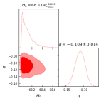
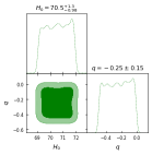
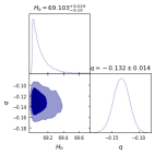
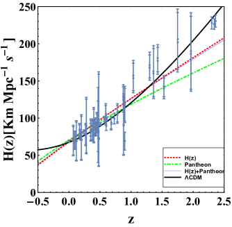
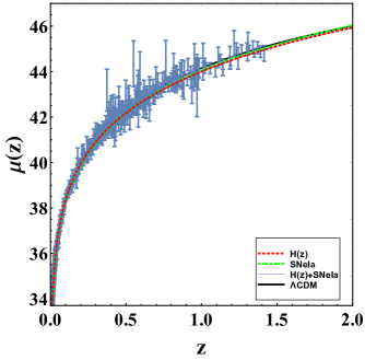
For a flat universe, we evaluate the best values of fit of $H_{0}$ and $q$ for the $H(z)$, Pantheon, and their joint data sets, respectively. For this purpose, we perform the coding in Python, where we use the Monte Carlo Markov chain (MCMC) method which is given in the Python module “emcee”, and plot the 2-D plots with $1-\sigma$, $2-\sigma$ likelihood contours. For the $H(z)$ data set, the value of best fit is $H_{0}=68.119_{-0.12}^{+0.028}$ and $q=-0.109_{-0.014}^{+0.014}$ (see Fig. 1a). In Fig. 1b, we can see that for the $Pantheon$ data set, the value of best fit is $H_{0}=70.5_{-0.98}^{+1.3}$ and $q=-0.25_{-0.15}^{+0.15}$. For the joint data set, we obtain the value of best fit of $H_{0}=69.103_{-0.10}^{+0.019}$ and $q=-0.132_{-0.014}^{+0.014}$, which is observed in Fig. 1c. In our work, we notice that $q_{0}$ differs from is not very close to -0.5, which is the approximate value for the $\Lambda$CDM model. In the refs [55, 56], it is pointed out that modified gravity theories could admit different values for $q_{0}$. With these best fit values, we plot the error bar plots for the Hubble data set and SNeIa data set. In Fig. 2, one can compare the present model with the $\Lambda$CDM model.

(a)

(b)

Figure 2: The error bar plots for $OHD$ and SNeIa data sets show the alikeness between our model and $\Lambda$CDM.

IV.1 Physical Parameters $\rho$, $p$ and $\omega$

In this section, we analyse the changing behaviour of energy density $\rho$ and pressure $p$. From Eqs. (15) and (16), it is clear that the values of $\rho$ and $p$ are in the terms of $z$ and the value of $\omega$ is in terms of $q$ only, i.e, a constant. So to understand the evolution of these parameters we plot the graphs.

(a)

(b)

(c)

Figure 3: The plots of $\rho$, $p$ and $\omega$ against redshift $z$

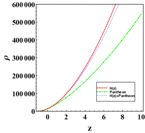
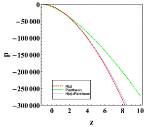
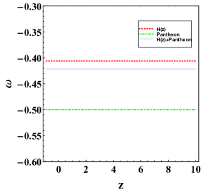
Fig. 3a shows the evolution of the energy density against the redshift. For high redshift $\rho$ is very large, and as $z$ decreases, $\rho$ also decreases for the whole range of $z$. As $z\to-1$, the energy density $\rho\to 0$. Further, Fig. 3b shows the evolution of pressure $p$ against redshift $z$, and we observe that the pressure is negative, which corresponds to accelerated expansion.

From Eqs. (15), (16) and (17), we calculate the present value of the EoS parameter $\omega$ as -0.406, -0.5, -0.421 for the $H(z)$, $Pantheon$ and their joint data sets, respectively. These values of the EoS parameter show that at present our model is in the quintessence region (see Fig. 3c).

IV.2 Energy Conditions

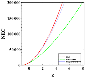
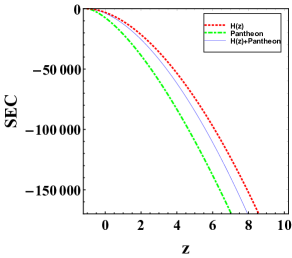
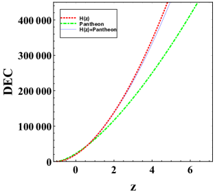
Energy conditions (EC’s) have relevance to singularities in general relativity. We wish to deduce the energy conditions for $f(R,G)$ modified gravity [31]. Using the expressions for the energy density and pressure that we derived earlier, we find that the NEC (null energy condition), WEC (weak energy condition), SEC (strong energy condition), and DEC (dominant energy condition) are given by:

• NEC $\Leftrightarrow$ $\rho+p\geq 0$,

• WEC $\Leftrightarrow$ $\rho\geq 0$, $\rho+p\geq 0$,

• SEC $\Leftrightarrow$ $\rho+3p\geq 0$, $\rho+p\geq 0$,

• DEC $\Leftrightarrow$ $\rho\geq 0$ , $\rho\pm p\geq 0$,

These connditions are illustrated in fig. 4. The NEC and DEC are satisfied, but the SEC is violated, in keeping with the idea of accelerated expansion of the universe.

(a)

(b)

(c)

Figure 4: Plots of NEC, WEC, DEC and SEC

IV.3 Cosmographic Parameters

To understand the universe’s expansion history, many cosmological parameters are studied, which are expressed in the form of higher order derivatives of the scala factor. Therefore, to explore the dynamics of the universe, these parameters are very helpful. For example Hubble parameter $H$ shows the expansion rate of the universe, the deceleration parameter $q$ tells about the phase transition of the universe, the jerk parameter $j$, snap parameter $s$ and lerk parameter $m$ investigate dark energy models and their dynamics. These are defined as:

$$H=\frac{\dot{a}}{a};~{}~{}q=-\frac{\ddot{a}}{aH^{2}};~{}~{}j=\frac{\dddot{a}}{aH^{3}};~{}~{}s=\frac{\ddddot{a}}{aH^{4}};~{}~{}l=\frac{\ddddot{\dot{a}}}{aH^{5}};~{}~{}m=\frac{\ddddot{\ddot{a}}}{aH^{4}}.$$ (25)

These parameters may also be written in terms of $q$ as

$$j=q(1+2q);~{}~{}s=-q(1+2q)(2+3q);~{}~{}l=q(2+3q)(1+2q)(3+4q);~{}~{}m=-q(2+3q)(1+2q)(3+4q)(4+5q).$$ (26)

Here $j$, $s$, $l$ and $m$ are known as the cosmographic parameters. Using the obtained best fit value of $q$, we find that the present value of $j=-0.085238,~{}~{}-0.125,~{}-0.097152$ for the $H(z)$, $Pantheon$ and $H(z)+Pantheon$ data sets, respectively.

IV.4 Statefinder Diagnostic

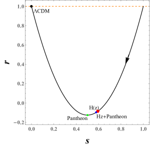
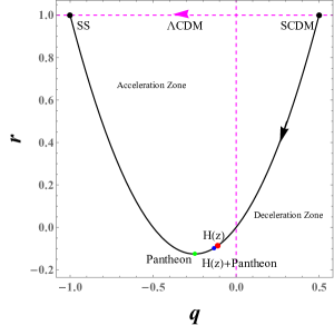
In the literature, we find that to understand the universe’s dynamics, geometric parameters play a very important role. When we study the deceleration parameter, we get information about the phase transition of the universe from deceleration to acceleration or vice versa. Therefore, it is required to study an additional higher order derivatives of $a$, viz. $r$. To study dark energy models, a statefinder diagnostic technique (SFD), is available [57, 58]; the pair is denoted by $\{r,s\}$. This pair, written in terms of $q$ is:

(a)

(b)

Figure 5: The $s-r$ and $q-r$ plots.

$$r=\frac{\dddot{a}}{H^{3}a}=2q^{2}+q\text{, \ \ }s=\frac{-1+r}{3(-\frac{1}{2}+q)},$$ (27)

where $q\neq\frac{1}{2}$.

Now, by using the statefinder diagnostic approach, we comment upon the behaviour of the model and also the diverging or converging behaviour of our model with respect to the $SCDM$ and $\Lambda CDM$ models. From observed values of $q$, we can calculate the values of $s$, and $r$ parameters. We notice that our model does not fit well for the $H(z)$ and $Pantheon$ data sets, and therefore we obtain the notable changes in the values’s best-fit for $r$ and $s$ (see Fig. 5a). Here, we see that our model approaches the $\Lambda CDM$ model as $q\to-0.5$.

IV.5 Om Diagnostic

Here, we use the $Om$ diagnostic technique known to compare our model with the $\Lambda CDM$ model. This helps us to separate various models of dark energy without calculating the energy density and the EoS parameter. The pattern of the trajectories in the $Om$ diagnostic plot gives an indication of the various dark energy models. The definition of the $Om$ diagnostic in terms of $z$ is:

$$Om(z)=\frac{\{\frac{H(z)}{H_{0}}\}^{2}-1}{z^{3}+3z^{2}+3z}.$$ (28)

Figure 6: The plot for om diagnostic.

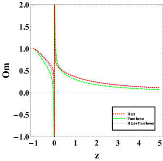
The plots of the $Om$ diagnostic helps us to explain the nature of dark energy models. We know that if the curvature is positive $z$, then the model is a ghost dark energy model, if the curvature is negative with respect to $z$, we have quintessence, and if it has zero curvature, then the model represents the $\Lambda CDM$ model. Fig. 6 shows that in late times, we have quintessence since the curvature is negative w.r.t. $z$ [59, 60].

V Conclusions

The late-time behaviour of our flat FLRW model in $f(R,G)$ gravity has been studied, where $F(R,G)=R+\alpha e^{-G}$ and the invariant $G$ is $G=R^{2}-4R_{\mu\nu}R^{\mu\nu}+R_{\mu\nu\alpha\zeta}R^{\mu\nu\alpha\zeta}$. Since the field equations are difficult to solve in general, we assume a power law for the scale factor $a$. We constrain $H$ and $q$ using observational datasets that are recent with the $MCMC$ methodology and then proceeded to study the behaviour of the obtained model, and the universe’s evolution. The model has exhibits a singularity that is of the point-type. The volume increases as $t$ increases. The Hubble parameter monotonically decreases as $z\rightarrow-1$. The model is expanding with constant acceleration. The energy density of the model monotonically decreases with an increase in time, starting from infinity and at late times, it tends to zero . Fig. 3, shows that our model is a quintessence dark energy model for all observational datasets .

The deceleration parameter is considered as a free model parameter and its present values are constrained as $q=-0.109_{-0.014}^{+0.014}$, $q=-0.25_{-0.15}^{+0.15}$, and $q=-0.132_{-0.014}^{+0.014}$ using $H(z)$, $Pantheon$, and $H(z)+Pantheon$ data sets, respectively, which deviate from the present day best fit values (see Fig. 1). The NEC and DEC energy conditions are satisfied, but the SEC does not hold for all the observational data sets, which support quintessence. The stability of this model is verified by the parameters, as illustrated in (see Fig. 4). The late time acceleration of the universe in supported by a violation of the SEC. The present value of the jerk cosmographic parameter is $j=-0.085238,~{}-0.125,~{}-0.097152$ for the data sets $H(z)$, $Pantheon$ and $H(z)+Pantheon$, respectively. This deviates from that of the $\Lambda$CDM. Our model has a quintessence type behaviour at late times. This is shown in the figure of $Om(z)$ which is convex with respect to the $z$-axis and shows stability during the evolution of the universe up to late times except at present (see Fig. 6). Now, by using the statefinder diagnostic approach, we investigated the behaviour of the model and also checked the and divergence and convergence of our model with respect to the $SCDM$ and $\Lambda CDM$ models. From the observed values of $q$, we can calculate the values of $s$, and $r$ parameters. It is noticed that the power law scale faactor does not fit well for $H(z)$ and $Pantheon$ data, and therefore we get the various changes in the values that are best-fit for $s$ and $r$ (see Fig. 5a). Here, it can also be seen that our model approaches $\Lambda CDM$ model as $q\to-0.5$ (see Fig. 5).

Thus, after reviewing the obtained results of our model, we see that our model starts with a singularity that is point like, and behaves like a expanding accelerated dark energy model that is of the quintessence type now but tends to the to the $\Lambda$CDM model at late times.

Acknowledgements The authors express their thanks to Prof. Sushant G. Ghosh, CTP, Jamia Millia Islamia, New Delhi, India for fruitful discussions and suggestions.

References

- [1] G. Cognola, M. Gastaldi and S. Zerbini, Int. J. Theor. Phys. 47, 898-910 (2008).
- [2] S. Nojiri, S. D. Odintsov and P. V. Tretyakov, Prog. Theor. Phys. Suppl. 172 (2008), 81-89.
- [3] K. Bamba, [arXiv:1504.04457 [gr-qc]].
- [4] S. D. Odintsov, V. K. Oikonomou and S. Banerjee, Nucl. Phys. B 938, 935-956 (2019).
- [5] F. G. Alvarenga, A. de la Cruz-Dombriz, M. J. S. Houndjo, M. E. Rodrigues and D. Sáez-Gómez, Phys. Rev. D 87, no.10, 103526 (2013). [erratum: Phys. Rev. D 87, no.12, 129905 (2013)]
- [6] M. Sharif and M. Zubair, JCAP 03 (2012), 028.
- [7] M. J. S. Houndjo, Int. J. Mod. Phys. D 21, 1250003 (2012).
- [8] M. Jamil, D. Momeni, M. Raza and R. Myrzakulov, Eur. Phys. J. C 72, 1999 (2012).
- [9] Z. Yousaf, K. Bamba and M. Z. u. H. Bhatti, Phys. Rev. D 93, no.12, 124048 (2016).
- [10] N. Godani, Int. J. Geom. Meth. Mod. Phys. 16, no.02, 1950024 (2018).
- [11] M. E. S. Alves, P. H. R. S. Moraes, J. C. N. de Araujo and M. Malheiro, Phys. Rev. D 94, no.2, 024032 (2016).
- [12] N. K. Sharma and J. K. Singh, Int. J. Theor. Phys. 53, no.9, 2912-2922 (2014).
- [13] R. Nagpal, J. K. Singh and S. Aygün, Astrophys. Space Sci. 363, 114 (2018).
- [14] Z. Yousaf, M. Ilyas and M. Z. Bhatti, Mod. Phys. Lett. A 32, no.30, 1750163 (2017).
- [15] A. Das, F. Rahaman, B. K. Guha and S. Ray, Eur. Phys. J. C 76, no.12, 654 (2016).
- [16] J. K. Singh and N. K. Sharma, Int. J. Theor. Phys. 53, 1424-1433 (2014).
- [17] R. Nagpal, S. K. J. Pacif, J. K. Singh, K. Bamba and A. Beesham, Eur. Phys. J. C 78, no.11, 946 (2018).
- [18] B. Li, J. D. Barrow and D. F. Mota, Phys. Rev. D 76, 044027 (2007).
- [19] S. Nojiri and S. D. Odintsov, Phys. Lett. B 631, 1-6 (2005).
- [20] S. Nojiri, S. D. Odintsov and O. G. Gorbunova, J. Phys. A 39, 6627-6634 (2006).
- [21] G. Cognola, E. Elizalde, S. Nojiri, S. D. Odintsov and S. Zerbini, Phys. Rev. D 73, 084007 (2006).
- [22] E. Elizalde, R. Myrzakulov, V. V. Obukhov and D. Saez-Gomez, Class. Quant. Grav. 27, 095007 (2010).
- [23] K. Izumi, Phys. Rev. D 90, no.4, 044037 (2014).
- [24] V. K. Oikonomou, Astrophys. Space Sci. 361, no.7, 211 (2016).
- [25] K. Kleidis and V. K. Oikonomou, Int. J. Geom. Meth. Mod. Phys. 15, no.04, 1850064 (2017).
- [26] V. K. Oikonomou, Phys. Rev. D 92, no.12, 124027 (2015).
- [27] A. Escofet and E. Elizalde, Mod. Phys. Lett. A 31, no.17, 1650108 (2016).
- [28] A. N. Makarenko and A. N. Myagky, Int. J. Geom. Meth. Mod. Phys. 14, no.10, 1750148 (2017).
- [29] K. Bamba, A. N. Makarenko, A. N. Myagky and S. D. Odintsov, Phys. Lett. B 732 (2014), 349-355.
- [30] A. N. Makarenko, Int. J. Geom. Meth. Mod. Phys. 13, no.05, 1630006 (2016).
- [31] N. Montelongo Garcia, F. S. N. Lobo, J. P. Mimoso and T. Harko, J. Phys. Conf. Ser. 314 (2011), 012056.
- [32] D. Lohiya and M. Sethi, Class. Quant. Grav. 16, 1545-1563 (1999).
- [33] M. Sethi, A. Batra and D. Lohiya, Phys. Rev. D 60, 108301 (1999).
- [34] A. Batra, D. Lohiya, S. Mahajan and A. Mukherjee, Int. J. Mod. Phys. D 9, no.06, 757-773 (2000).
- [35] S. Gehlaut, A. Mukherjee, S. Mahajan and D. Lohiya, Spacetime and Substance 14 (2002), 152.
- [36] S. Gehlaut, P. K. Geetanjali and D. Lohiya, [arXiv:astro-ph/0306448 [astro-ph]].
- [37] A. Dev, D. Jain and D. Lohiya, [arXiv:0804.3491 [astro-ph]].
- [38] A. Dev, M. Safonova, D. Jain and D. Lohiya, Phys. Lett. B 548, 12-18 (2002).
- [39] Z. H. Zhu, M. Hu, J. S. Alcaniz and Y. X. Liu, Astron. Astrophys. 483 (2008), 15
- [40] G. Sethi, A. Dev and D. Jain, Phys. Lett. B 624, 135-140 (2005).
- [41] D. L. Shafer, Phys. Rev. D 91, no.10, 103516 (2015) doi:10.1103/PhysRevD.91.103516 [arXiv:1502.05416 [astro-ph.CO]].
- [42] J. K. Singh, H. Balhara, K. Bamba and J. Jena, JHEP 03 (2023), 191.
- [43] J. K. Singh, Shaily, S. Ram, J. R. L. Santos and J. A. S. Fortunato, Int. J. Mod. Phys. D, doi:10.1142/S021827182350040 [arXiv:2209.06859 [gr-qc]].
- [44] J. K. Singh, K. Bamba, R. Nagpal and S. K. J. Pacif, Phys. Rev. D 97 (2018) no.12, 123536.
- [45] H. Shabani and A. H. Ziaie, Eur. Phys. J. C 77 (2017) no.1, 31.
- [46] S. Rani, A. Altaibayeva, M. Shahalam, J. K. Singh and R. Myrzakulov, JCAP 03 (2015), 031
- [47] S. Kumar, Mon. Not. Roy. Astron. Soc. 422 (2012), 2532-2538.
- [48] Shaily, M. Zeyauddin and J. K. Singh, [arXiv:2207.05076 [gr-qc]].
- [49] D. M. Scolnic et al. [Pan-STARRS1], Astrophys. J. 859, no.2, 101 (2018).
- [50] A. G. Riess, R. P. Kirshner, B. P. Schmidt, S. Jha, P. Challis, P. M. Garnavich, A. A. Esin, C. Carpenter, R. Grashius and R. E. Schild, et al. Astron. J. 117, 707-724 (1999).
- [51] S. Jha, R. P. Kirshner, P. Challis, P. M. Garnavich, T. Matheson, A. M. Soderberg, G. J. M. Graves, M. Hicken, J. F. Alves and H. G. Arce, et al. Astron. J. 131, 527-554 (2006).
- [52] M. Hicken, P. Challis, S. Jha, R. P. Kirsher, T. Matheson, M. Modjaz, A. Rest and W. M. Wood-Vasey, Astrophys. J. 700, 331-357 (2009).
- [53] C. Contreras, M. Hamuy, M. M. Phillips, G. Folatelli, N. B. Suntzeff, S. E. Persson, M. Stritzinger, L. Boldt, S. Gonzalez and W. Krzeminski, et al. Astron. J. 139, 519-539 (2010).
- [54] M. Sako et al. [SDSS], Publ. Astron. Soc. Pac. 130, no.988, 064002 (2018).
- [55] C. P. Singh and M. Srivastava, Eur. Phys. J. C 78, no.3, 190 (2018)
- [56] S. K. Sahu, S. K. Tripathy, P. K. Sahoo and A. Nath, Chin. J. Phys. 55, 862-869 (2017)
- [57] V. Sahni, T. D. Saini, A. A. Starobinsky and U. Alam, JETP Lett. 77, 201-206 (2003).
- [58] U. Alam, V. Sahni, T. D. Saini and A. A. Starobinsky, Mon. Not. Roy. Astron. Soc. 344, 1057 (2003).
- [59] J. K. Singh and R. Nagpal, Eur. Phys. J. C 80 (2020) no.4, 295.
- [60] J. K. Singh, A. Singh, G. K. Goswami and J. Jena, Annals Phys. 443 (2022), 168958.