COMAP Early Science: VIII. A Joint Stacking Analysis with eBOSS Quasars

Abstract

We present a new upper limit on the cosmic molecular gas density at $z=2.4-3.4$ obtained using the first year of observations from the CO Mapping Array Project (COMAP). COMAP data cubes are stacked on the 3D positions of 282 quasars selected from the Extended Baryon Oscillation Spectroscopic Survey (eBOSS) catalog, yielding a 95% upper limit for flux from CO(1-0) line emission of 0.210 Jy km/s. Depending on the assumptions made, this value can be interpreted as either an average CO line luminosity $L^{\prime}_{\mathrm{CO}}$ of eBOSS quasars of $\leq 7.30\times 10^{10}$ K km pc² s^-1, or an average molecular gas density $\rho_{\mathrm{H_{2}}}$ in regions of the universe containing a quasar of $\leq 2.02\times 10^{8}$ M_⊙ cMpc^-3. The $L^{\prime}_{\mathrm{CO}}$ upper limit falls among CO line luminosities obtained from individually-targeted quasars in the COMAP redshift range, and the $\rho_{\mathrm{H_{2}}}$ value is comparable to upper limits obtained from other Line Intensity Mapping (LIM) surveys and their joint analyses. Further, we forecast the values obtainable with the COMAP/eBOSS stack after the full 5-year COMAP Pathfinder survey. We predict that a detection is probable with this method, depending on the CO properties of the quasar sample. Based on these achieved sensitivities, we believe that this technique of stacking LIM data on the positions of traditional galaxy or quasar catalogs is extremely promising, both as a technique for investigating large galaxy catalogs efficiently at high redshift and as a technique for bolstering the sensitivity of LIM experiments, even with a fraction of their total expected survey data.

1 Introduction

Spectral Line Intensity Mapping (LIM) is an emerging observational technique with the potential to enhance our understanding of the universe by constraining the global properties of galaxies over cosmic time. LIM surveys do not aim to resolve individual galaxies, but instead measure 3-dimensional fluctuations in the integrated emission from many galaxies, allowing for efficient mapping of galaxies across large cosmic volumes (see Kovetz et al., 2019, for a review). Because LIM measures integrated emission, it is sensitive to the faintest galaxies, which are nearly impossible to detect in traditional surveys but nevertheless make up the bulk of the galaxy population at any given cosmic time. Observationally, the field is still in its early stages, with dedicated LIM instruments only beginning to publish early autocorrelation constraints (eg. COMAP, Cleary et al. 2022; the Hydrogen Epoch of Reionization Array, HERA, Abdurashidova et al. 2022; and MeerKAT Paul et al. 2023).

Currently, the results being released from these first LIM surveys are primarily upper limits (for COMAP, Chung et al., 2022) and are not yet sufficient to achieve the measurements described above. This is partially a consequence of the newness of the field – strong autocorrelation detections of a given spectral line are required to measure its cosmological fluctuations, and most LIM surveys have simply not been integrating long enough to achieve the needed sensitivities (for example, COMAP projects a secure autocorrelation detection after 5 years; Chung et al., 2022). However, cosmic line emission may be detectable even with present-day LIM datasets, if careful signal processing techniques making use of external datasets are applied.

In particular, averaging together intensity-map voxels (3D pixels) that are known to contain galaxies (by comparison with some other survey) in a stacking analysis has the potential to make a detection of the average CO line temperature associated with catalog galaxies, even with an intensity map insufficiently sensitive for other analyses (Silva et al., 2021). Stacking, or coadding, is an established technique for improving sensitivity in traditional, targeted galaxy surveys (e.g., Stanley et al., 2019; Jolly et al., 2021; Romano et al., 2022; Lujan Niemeyer et al., 2022), and has recently been extended to LIM observations as well (Keenan et al., 2022). The efficacy of this technique will depend on factors such as the number of traditional survey objects that fall into the LIM survey footprint, and the redshift accuracy in the traditional catalog (Chung et al., 2019; Silva et al., 2021), as well as the chosen weighting scheme (Sinigaglia et al., 2022).

In this paper, we use LIM data from the CO Mapping Array Project (COMAP; Cleary et al., 2022), the first survey to use a purpose-built instrument (the COMAP Pathfinder, described in detail in Lamb et al., 2022), to impose direct constraints on the clustering-scale CO power spectrum at high redshifts. We use COMAP Season 1 data, taken during the first 13-month observing season of the project. COMAP observations cover a frequency range of 26–34 GHz (redshifts of $z=2.4$–$3.4$) and encompass three $\sim 4$ deg² fields. The data reduction and map-making processes for these Season 1 data are described in Foss et al. (2022), while power spectrum estimation techniques and constraints are described in Ihle et al. (2022) and Chung et al. (2022). Observations are continuing with the Pathfinder, to complete the nominal 5-year survey, at the end of which a detection of the CO auto-power spectrum is forecast. The COMAP fields were selected to overlap with the HETDEX survey of Ly-$\alpha$ emitters (Gebhardt et al., 2021), allowing us to perform stacking and cross-correlation analyses of these two datasets.

As a preliminary step, we investigate in this work the potential for the BOSS/eBOSS quasar sample (Dawson et al., 2016) to provide additional constraints and inform our understanding of the relationship between active galaxies and star formation. The eBOSS catalog was developed with the intention of studying the Ly$\alpha$ forest and therefore covers a redshift range overlapping with that of COMAP – the eBOSS DR16 catalog includes spectroscopic observations of $>239,000$ quasars in the range $z>2.1$. Depending on the assumptions made, a stack of COMAP data on the positions of eBOSS quasars can be treated as a measurement of either the average CO luminosity of the quasars themselves or the average molecular gas density at quasar positions.

In addition to its extensive size, which allows for a high-sensitivity stack, the combination of COMAP with the eBOSS catalog enables the study of the CO properties of a large sample of high-redshift quasars. Quasar feedback, particularly in relation to the molecular gas traced by CO transitions, is poorly understood on a statistical scale. Current studies mainly involve individual objects, using the CO rotational ladder in the host galaxies of Active Galactic Nuclei (AGN) to study the effects of AGN on their surroundings. These are complex measurements requiring extremely CO-bright objects, and thus the pool of available galaxies for study is small and biased, especially at high redshifts. LIM measurements will be able to provide a more complete picture of the wider population of AGN and their host galaxies (e.g., Breysse & Alexandroff, 2019).

In this work, we will investigate the CO properties of the 282 eBOSS quasars in the COMAP fields through stacking, thus providing constraints on the molecular gas content of a large sample of high-redshift quasars for the first time. We will additionally use this analysis to explore the viabilty of stacking as a LIM technique. As such, we will forecast the sensitivity of the full five-year COMAP Pathfinder survey to CO emission from the eBOSS quasars. Section 2 introduces both the COMAP Pathfinder (§2.1) and eBOSS surveys (§2.2), and Section 3 describes the stacking methodology we use in our analysis. We present the results of the stacking analysis in Section 4, and forecast the results of stacking the full Pathfinder survey (§4.2). We discuss the implications of these results in Section 5.

We assume a $\Lambda$CDM cosmology based broadly on nine-year WMAP (Hinshaw et al., 2013) results throughout, with $\Omega_{\mathrm{m}}=0.286$, $\Omega_{\Lambda}=0.714$, $\Omega_{\mathrm{b}}=0.047$, and $H_{0}=100h\mathrm{km\ s^{-1}\ Mpc^{-1}}$ with $h=0.7$. These are the same values used in all previous COMAP works. Where necessary, distances are given as proper values.

2 Data

2.1 COMAP

The COMAP Season 1 data consist of 13 months of observations using the COMAP Pathfinder instrument, a single-polarization 19-feed spectrometer array fielded on a 10.4 m telescope located at the Owens Valley Radio Observatory (OVRO) in California (the Pathfinder is described in detail in Lamb et al. 2022). The Pathfinder instrument observes between 26 and 34 GHz, and is therefore sensitive to the CO(1–0) rotational transition ($\nu_{0}=115.27$ GHz) emitted in a redshift range of $z=2.4-3.4$. These observations were towards three $\sim 4$-deg² cosmological fields (shown in Table 1).

Table 1: The locations of the three fields used in the COMAP Pathfinder survey.

Field	RA (J2000)	Dec (J2000)
Field 1	01h 41m 44$\fs$4	00$\arcdeg$ 00$\arcmin$ 00$\farcs$0
Field 2	11h 20m 00$\fs$0	52$\arcdeg$ 30$\arcmin$ 00$\farcs$0
Field 3	15h 04m 00$\fs$0	55$\arcdeg$ 00$\arcmin$ 00$\farcs$0

During observations, the telescope is positioned at the leading edge of the field and performs a scanning motion while the cosmological field drifts through. This usually takes 3–10 minutes, after which the telescope is pointed to the leading edge of the field again and the procedure is repeated. This means that over time, we are scanning the fields from several different directions leading to a smoothly varying noise distribution in the final maps, with low noise in the central regions of the field, and gradually increasing levels of noise towards the edges of the fields.

Raw time-ordered data (TOD) from the telescope are processed by applying a series of filters with the goal of removing correlated noise, standing waves, continuum foregrounds, ground contamination and other systematic effects from the TOD. This process and the COMAP scanning strategies are described in detail by Foss et al. (2022). The output of this pipeline is a set of three calibrated three-dimensional intensity maps, each of angular size $\sim 4$ deg² with 31.25 MHz spectral resolution and a 4.9–4.4 arcmin beam FWHM. At small scales these maps are dominated by uncorrelated, Gaussian noise (Foss et al., 2022). The maps are somewhat elongated in the right ascension direction, giving us appreciable coverage in a 3D region with dimensions (in comoving coordinates) roughly 300 Mpc $\times$ 200 Mpc in directions perpendicular to the line of sight (at redshift $z=2.9$) and about 1000 Mpc along the line of sight, for a total volume of the order 6$\times 10^{7}$ Mpc³ comoving for each field.

As described by Foss et al. (2022), Ihle et al. (2022) and Rennie et al. (2022), the maps are calibrated to the total power entering the telescope. About 72 % of this power comes from the main beam, with another roughly 10 % of the power in the near sidelobes (within about 30 arcmin). To take this scale-dependence into account Ihle et al. (2022) use a model of the COMAP beam to construct a beam transfer function for the power spectrum. For the purposes of our stacking analysis, since we are mostly interested in the smallest scales in the map, we simply divide the map (and the corresponding uncertainty map) by a single overall factor of 0.72 to get the right calibration at scales corresponding to the main beam.

2.2 eBOSS

The Baryon Oscillation Spectroscopic Survey (BOSS; Dawson et al. 2013) and its extension (eBOSS; Ahumada et al. 2020) together encompass eleven years of observations using the BOSS spectrograph at Apache Point Observatory (Gunn et al., 2006; Smee et al., 2013). We use the large ($\sim 240000$-object) eBOSS spectroscopic sample of Quasi-Stellar Objects (QSOs) at $z\geq 2.4$, which was intended to enable studies of the Ly$\alpha$ forest at $z\sim 1$. These observations targeted objects that were selected based on WISE/SDSS DR13 imaging data. We use the eBOSS DR16 superset catalog (Lyke et al., 2020; Ahumada et al., 2020), released in 2020 – the final iteration of the BOSS/eBOSS catalog. While principally composed of traditional quasars, the superset applied no quasar-selection pipeline and thus contains a small percentage (3.3%, in the overlap with COMAP fields) of bright galaxies, broad absorption line quasars, and damped Ly$\alpha$ systems.

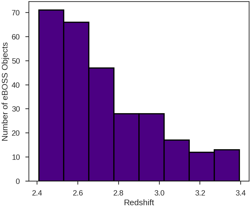
Figure 1: The redshift distribution of the eBOSS objects used for this stacking analysis.

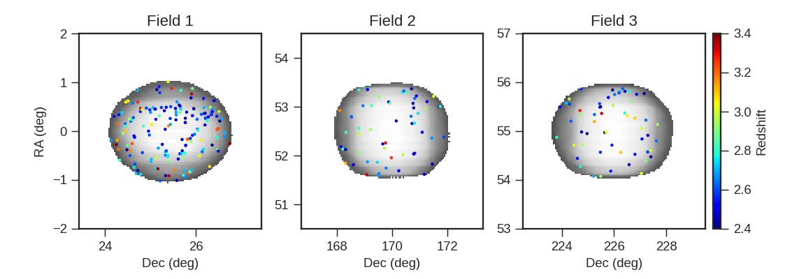
Figure 2: The distribution in space and redshift of the eBOSS objects used for this stacking analysis, plotted on the COMAP Season 1 median map RMS for each field (see Foss et al., 2022).

Objects in the eBOSS catalog are identified and their redshifts are determined simultaneously, through the fitting of templates spanning galaxies, quasars, and stars to the eBOSS spectra (stepping over redshift; Bolton et al., 2012). Spectra are optical, and at the redshifts of interest the templates to be fit typically include some combination of Ly$\alpha$, H$\alpha$ and H$\beta$, and a range of optical and NUV forbidden metal lines. The fit with the minimum reduced-$\chi^{2}$ value is used, provided $\chi_{r}^{2}>0.01$ and there is no other similarly confident fit determination greatly offset in redshift from the best-fit value. Visual followup is used to confirm the least confident identifications, and to test the algorithmic determination. Tests of the classification algorithm on blank-sky spectra showed a $<2$% false positive rate – the eBOSS redshift determinations are generally considered highly trustworthy. Based on the pixel size of the detector, the uncertainty in the eBOSS redshifts is at most $\sim 207\ \mathrm{km}\ \mathrm{s}^{-1}$, or $|\Delta z|\leq 0.01$ (Bautista et al., 2017) (approximately 1 COMAP channel). We note that this uncertainty does not account for the systematic gas in- or outflows that may be present in quasars; we discuss this additional consideration in §4.1.

In total, 282 eBOSS objects lie in the COMAP fields, after duplicates are removed. The average redshift of these objects is $z=2.73$, with their redshift distribution as shown in Figure 1. Their spatial distribution is shown in Figure 2, against the COMAP Season 1 sensitivity.

3 Stacking Methods

While the general philosophy behind a stacking analysis is simple – objects in the galaxy catalog are located in 3D space in the LIM map, some 3D region of the map centered around the catalog object is clipped from the map (a ‘cubelet’), these cubelets are coadded together, and a final flux measurement is read out from the resulting stack – there are many subtleties to consider when actually implementing the technique. In particular, we wish to ensure that the cut-out cubelets are centered as precisely as possible on the catalog objects’ positions in the 3D COMAP data cube, to mitigate the effects of beam dilution from incorporating empty regions of space into the surface brightness density calculations.

Other subtleties to consider when stacking include the extremely asymmetric noise response (the RMS noise in each COMAP spaxel, or two-dimensional ‘spatial pixel’, is orders of magnitude larger at the edges of the maps), and the response of the maps (and thus the stack) to the data reduction pipeline (discussed in §2.1), which is designed to remove low-order Fourier modes (i.e. large scales) in both the spatial and spectral axes (as illustrated by Figure 5 of Ihle et al. 2022).

3.1 Cutting out and Indexing

For each catalog object, we clip a 3D cubelet with dimensions 42 arcmin $\times$ 42 arcmin $\times$ 1.28 GHz from the LIM map. These cubelets are purposefully large compared to the COMAP spatial and spectral resolution, in order to search visually for potential large-scale fluctuations in the stack. To determine the average intensity of the stacked objects themselves, a much smaller 3D aperture is chosen to sum over. We take this aperture to be about $1.5$ times the size of the COMAP main beam in the spatial axes (i.e., $6^{\prime}$), meaning that the catalog object could be located anywhere in its central spaxel and its entire beam FWHM will be included in the aperture. Thus, we avoid excluding any of the signal from the final determinations of the stack values, while still keeping the aperture as small as possible to mitigate the effects of beam dilution and maximize our signal-to-noise ratio (S/N). We make a similar determination in the spectral axis, including the three central frequency channels in the stack aperture ($93.75\ \mathrm{MHz}$). This corresponds to a velocity width $\sim 950$ km/s, roughly the largest CO linewidth that has been observed in similar eBOSS quasars in our redshift range (Riechers et al., 2011; Hill et al., 2019; Muñoz-Elgueta et al., 2022). Additionally, as many quasars have CO linewidths much smaller than this, this chosen spectral width allows for some velocity offset between the CO emission and the optical lines used to determine the eBOSS redshifts (see §4.1). Instrumental aliasing between adjacent COMAP science channels is negligible (Lamb et al., 2022).

We mask any map voxel with an integration time below 1000 seconds (50000 ‘hits’, a stricter cut than is taken for the overall COMAP pipeline; Foss et al. 2022). If an individual cubelet has its central voxel (i.e., the voxel actually containing the catalog object) masked, or more than half of the voxels in its smaller aperture masked, it is excluded from the stack.

3.2 Determining Physical Quantities from Cubelets

Before stacking together the CO fluxes of each individual catalog object, we calculate astrophysical values associated with these numbers, as values such as $z$, $\nu_{\mathrm{obs}}$, and $D_{\mathrm{L}}$ vary across the stack. These astrophysical quantities include the average CO line luminosity, $L^{\prime}_{\mathrm{CO}}$, and the average molecular gas density, $\rho_{\mathrm{H_{2}}}$. The COMAP data cubes are in brightness temperature units, so we begin by determining the frequency-integrated line flux $(S\Delta\nu)$ associated with each individual catalog object,

$$S\Delta\nu=\frac{2\nu^{2}k_{B}T_{b}}{c^{2}}\Omega_{\mathrm{beam}}\Delta\nu.$$ (1)

In this case, $T_{b}$ is the brightness temperature in each frequency channel, summed across the $3\times 3$ central aperture, $\Omega_{\mathrm{beam}}$ is the COMAP main beam solid angle, and $\Delta\nu$ is the channel width in km/s. We follow Solomon et al. (1997) to calculate $L^{\prime}_{\mathrm{CO}}$,

$$L^{\prime}_{\mathrm{CO}}=\frac{c^{2}}{2k_{B}}S\Delta\nu\frac{D_{\mathrm{L}}^{2}}{\nu_{\mathrm{obs}}^{2}(1+z)^{3}},$$ (2)

where $D_{L}$ is the luminosity distance of the catalog object. This is calculated in each frequency channel, and then the three frequency channels in the cubelet’s central aperture are summed over to obtain the final value. The line luminosity is then converted to a $\rho_{\mathrm{H_{2}}}$ value: the Bolatto et al. (2013) CO-to-H₂ conversion factor of $3.6\ M_{\odot}$(K km s^-1 pc²)^-1, calculated for the Milky Way, is used to calculate the associated molecular gas mass. These masses are divided by the comoving volume (for easy comparison with existing LIM values) of the stack aperture to calculate $\rho_{\mathrm{H_{2}}}$.

3.3 Stacking Cubelets

We then coadd the $S\Delta\nu$, $L^{\prime}_{\mathrm{CO}}$, and $\rho_{\mathrm{H_{2}}}$ values for each individual catalog object together to calculate the final stack values. To account for the inhomogeneous noise response across the map (§2.1), values are weighted by their RMS noise when averaging. All stacks are performed using inverse variance-weighting,

$$\hat{y}=\frac{\sum_{i}y_{i}/\sigma^{2}_{i}}{\sum_{i}1/\sigma^{2}_{i}},$$ (3)

for voxel value $y_{i}$ with RMS noise $\sigma_{i}$. They have standard deviation

$$\sigma_{y}=\sqrt{\frac{1}{\sum_{i}1/\sigma^{2}_{i}}}.$$ (4)

We take the assumption that the final value returned from the stack should be positive for the purposes of the upper limit. If, after all calculations are complete, the stack is returning a negative $S\Delta\nu$ value, it is cast to zero before the upper limit is calculated.

For the full cubelets used for visualization, we attempt to lessen the effect of any catalog asymmetries on the final stack by rotating each cubelet randomly in its spatial axes by either $0^{\circ}$, $90^{\circ}$, $180^{\circ}$, or $270^{\circ}$, before coadding the cubelets together using the same weighting scheme. For these visualization stacks, the coadding is performed voxel-by-voxel (i.e., weighted by the RMS uncertainty in each voxel).

This is the simplest possible version of a stack, ignoring other available information such as the significance of the catalog objects’ detections with eBOSS, or the optical luminosity of the catalog objects, both of which could also be used for weighting (see, for example, Sinigaglia et al., 2022). While we do plan to explore these techniques in the future, we assume for now that the noise in the Season 1 COMAP data cube is much greater than any variations across the eBOSS catalog.

3.4 Characterizing the stacked emission

3.4.1 Spatial bootstrap tests

While we believe the noise in our maps to be Gaussian-distributed (‘white’ noise: see §2.1, also Foss et al. 2022) over the entire map, this stacking analysis introduces a new sampling strategy, and it is possible that the white noise assumption does not hold under this new sampling. We therefore perform a spatial ‘bootstrap’ test on each stack to confirm the noise distribution in our maps, and to determine the uncertainty in each of the stacked values.

This is done by binning the actual eBOSS catalog by COMAP field and by redshift (into three redshift bins), and then generating an artificial catalog with the same overall redshift and field distribution as the real catalog but with random 3D positions. Variations in catalog number density between field, as well as instrumental effects such as the changing primary beam with frequency and potential systematic errors correlating to on-sky position, will thus appear both in the bootstrapped stacks and the real stack. The LIM map is then stacked on the artificial catalog. This is repeated for 10000 different random artificial catalog iterations for each real stack run, to fully characterize the stack noise response.

3.4.2 Simulation-based tests

As an end-to-end test of the stacking pipeline, we create mock COMAP observations of simulated cosmic CO signal, generate mock galaxy catalogs associated with these cubes, and perform the stacking analysis on these simulated data. Mock CO emission is generated by painting CO luminosities onto a dark matter halo catalog from peak-patch $N$-body simulations (Stein et al., 2019). We follow the COMAP fiuducial model presented by Chung et al. (2022) to determine CO luminosity as a function of halo mass,

$$\frac{L^{\prime}_{\mathrm{CO}}(M_{h})}{\mathrm{K\ km\ s^{-1}\ pc^{2}}}=\frac{C}{(M_{h}/M)^{A}+(M_{h}/M)^{B}},$$ (5)

where $C=10^{10.63}$, $A=-2.85$, $B=-0.42$, and $M=10^{12.3}$ M_⊙. Following Chung et al. (2022), we introduce a log-normal scatter with $\sigma=0.42$, and artificially broaden the CO emission line in each halo by an effective velocity $v_{\mathrm{eff}}$ based on the halo’s virial mass. To generate mock COMAP data cubes, we additionally beam-smooth the emission in the spatial axes, by convolving the mock cubes using a 2D Gaussian kernel with a 4-arcminute FWHM, to approximate the COMAP primary beam.

The artificial CO emission cube generated from these simulations is then converted into a timestream, scaled by a factor of 1000 to simulate an (unrealistically) strong detection, and added into real time-ordered data from the first COMAP observing season (Stutzer et al., in prep). The positions of the simulated halos should have no correlation with any existing real cosmic structure, so this is an excellent way to simulate observations with the actual noise structure that COMAP observes. This mock timestream is passed through the COMAP pipeline, so any effects of the several pipeline filters (Foss et al., 2022) will show up in the mock data cube.

In addition to the mock COMAP data cubes, we generate an artificial galaxy catalog by randomly selecting 282 dark matter halos from the most massive 30% of halos in the peak-patch catalog (dark-matter masses between $9\times 10^{13}\ \mathrm{M}_{\odot}$ and $4\times 10^{12}\ \mathrm{M}_{\odot}$), and taking these halos to be the objects emitting brightly enough in some other galaxy tracer to be detected in a traditional galaxy survey. Only the 3D positions of the halos are required for the stacking analysis, so we do not calculate any other mock parameters for the galaxy survey.

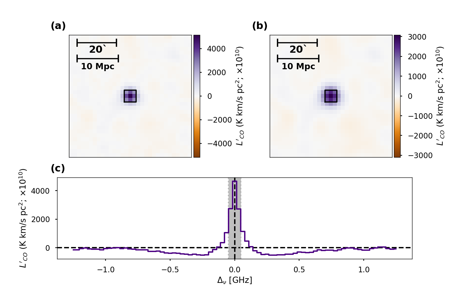
Figure 3: A simulated high-significance stacking detection. (a) The central three frequency channels coadded to provide a view of the spatial distribution of signal. The black box in the center indicates the smaller aperture used to calculate single stack values. (b) The same spatial representation of the stack, smoothed with a $4^{\prime}$ Gaussian kernel to approximate the COMAP primary beam. (c) The frequency spectrum of the stack. The value in each spectral channel is determined by summing over the spatial aperture indicated in (a). The three frequency channels making up the stack aperture are highlighted in grey.

We then run the stacking pipeline on three different realizations of the mock data cube and galaxy catalog. This is done principally to confirm that the COMAP pipeline is not attenuating the stacking signal in any unexpected ways, and to determine the size of the stacking aperture discussed in §3.1. An example of the resulting simulated stack, shown in Figure 3, confirms that the $6^{\prime}\times 6^{\prime}\times 93.75$ MHz aperture we selected indeed encloses the majority of the stacked flux ($\sim 80$%), without incorporating much empty space. We note that, on either side of the signal in the simulated spectrum, the $L^{\prime}_{\mathrm{CO}}$ value in each spectral channel dips below zero. We believe this to be an effect of the high-pass filtering used in the COMAP pipeline. We will explore this effect, and the effects of other simulation choices on the stack, in greater detail in future work.

4 Results

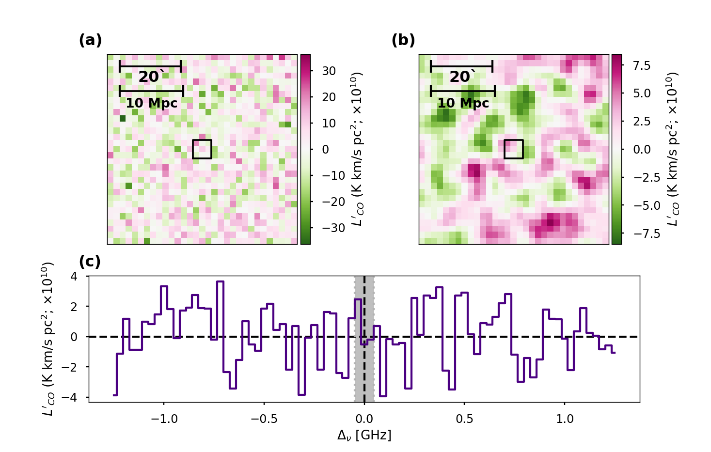
Figure 4: The result of stacking the COMAP data cubes on the 3D positions of eBOSS quasars. (a) The central three frequency channels coadded to provide a view of the spatial distribution of signal. The black box in the center indicates the smaller aperture used to calculate single stack values. (b) The same spatial representation of the stack, smoothed with a $4^{\prime}$ Gaussian kernel to approximate the COMAP primary beam. (c) The frequency spectrum of the stack. The value in each spectral channel is determined by summing over the spatial aperture indicated in (a). The three frequency channels making up the 3D stack aperture are highlighted in grey. All distance scales are given as proper values.

The final COMAP/eBOSS stack is shown in Figure 4. We find, at our current sensitivity level, no detection of CO emission associated with the 282 eBOSS quasars in the COMAP fields. We set a 95% upper limit on the CO frequency-integrated line flux of $S\Delta\nu$ $\leq 0.210$ Jy km/s, corresponding to a limit on the CO line luminosity of $L^{\prime}_{\mathrm{CO}}$$\ \leq 7.30\times 10^{10}\$K km pc² s^-1 and a limit on the average molecular gas density in regions containing a quasar of $\rho_{\mathrm{H_{2}}}$$\ \leq 2.02\times 10^{8}$ M_⊙ Mpc^-3.

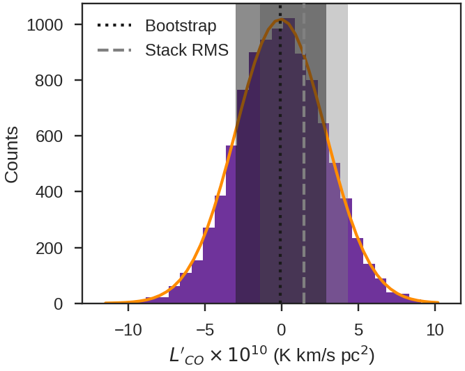
Figure 5: A histogram of the $L^{\prime}_{\mathrm{CO}}$ values returned from 10000 stacks performed on random 3D positions in the COMAP data cubes, with the same spectral and field distribution of objects as the real eBOSS catalog. A Gaussian fit to the histogram is shown in orange. The 66% confidence interval of the fitted Gaussian (i.e., 1 standard deviation about the fitted mean) is shown in dark gray. Overlaid in light gray is the actual COMAP/eBOSS stack value and its 1-$\sigma$ RMS uncertainty calculated directly from the map (see §3.3).

The COMAP/eBOSS bootstrap test is shown in Figure 5. As expected, the maps remain consistent with Gaussian noise centered at $T_{b}=0$ K even in this stacking analysis. As this is a more robust calculation of the distribution of stack values expected from random noise, we use the 95% confidence region calculated from a Gaussian fit to these bootstrapped $L^{\prime}_{\mathrm{CO}}$ values as the uncertainty in our stack.

In addition to the ¹²CO(1-0) transition for which COMAP was designed, we perform the stacking analysis on four other common molecular emission lines identified as potential COMAP foregrounds: the ¹³CO isotope’s $J=1\rightarrow 0$ rotational transition, the HCN $J=1\rightarrow 0$ transition, the CS $J=2\rightarrow 1$ transition, and the CN^- radical’s $J=1\rightarrow 0$ rotational transition. As expected, each of these stacks are also nondetections, although many are more sensitive than the ¹²CO(1-0) stack due to the increased density of eBOSS objects at lower redshifts. The resulting upper limits are shown in Table 2, and the full 3D stacked cubelets are shown in Appendix A.

Table 2: 95% upper limits obtained by stacking the COMAP data cube on the CO(1-0) line and expected foreground emission lines.

Spectral	# of	$\nu_{\mathrm{rest}}$	Redshift	$S\Delta\nu$ 95% Upper Limit	$L^{\prime}$ 95% Upper Limit
Line	Objects	(GHz)	Range	(Jy km s-1)	(K km pc2 s-1)
12CO(1-0)	282	115.27	$2.4-3.4$	$\leq 0.210$	$\leq 7.30\times 10^{10}$
12CO(1-0) with offset	280	115.15	$2.4-3.4$	$\leq 0.160$	$\leq 8.69\times 10^{10}$
HCN(1-0)	693	88.63	$1.6-2.4$	$\leq 0.171$	$\leq 5.62\times 10^{10}$
CS(2-1)	538	91.98	$1.7-2.5$	$\leq 0.120$	$\leq 4.71\times 10^{10}$
13CO(1-0)	345	110.20	$2.2-3.2$	$\leq 0.149$	$\leq 5.21\times 10^{10}$
CN-(1-0)	298	113.49	$2.3-3.4$	$\leq 0.262$	$\leq 9.08\times 10^{10}$

4.1 Offsets between optical and CO redshifts

Although the cataloged eBOSS redshifts are considered very precise, high-redshift quasars often contain large systematic outflows/inflows that could cause velocity offsets between optical emission lines, such as those used by eBOSS, and the CO emission, which traces the cold gas of the galaxy itself (Banerji et al., 2017; Herrera-Camus et al., 2020; Bischetti et al., 2021). This is an important consideration, as even small redshift uncertainties can cause significant attenuation in the signal of LIM/galaxy catalog cross-correlation analyses (Chung et al., 2019, 2021). The shot component of the cross-power spectrum (i.e., the cross power at small spatial scales, the most direct analogue to a stacking analysis) is where this effect is at its worst, although COMAP is most sensitive to larger spatial scales than those where attenuation due to redshift uncertainty is truly catastrophic.

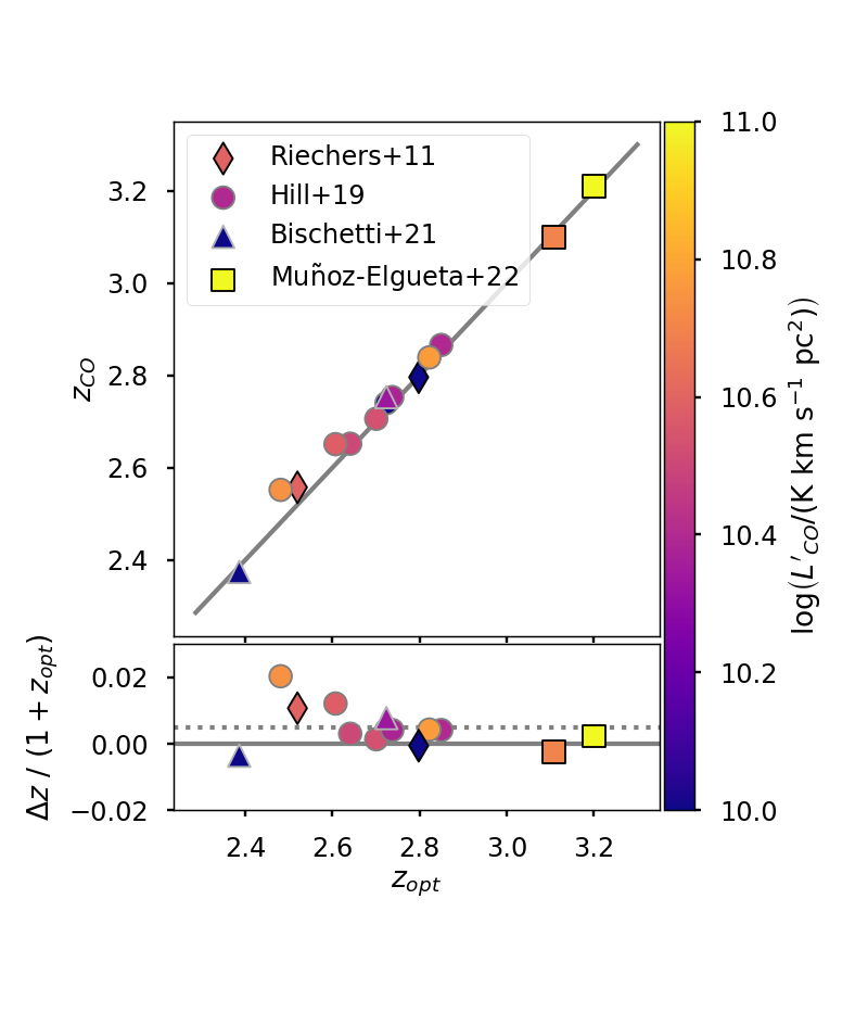
Figure 6: The optically-determined redshift values compared with CO-based redshifts for a selection of quasars individually detected in CO in the COMAP redshift range. The colourmap is the extrapolated CO(1-0) luminosity of each object, discussed in §5.1, and the line where $z_{\mathrm{opt}}=z_{\mathrm{CO}}$ is shown for reference. In the bottom panel we indicate the mean offset of the sample with a dotted line.

To quanitfy any systemic offsets between the cataloged redshift for our eBOSS sample ($z_{\mathrm{opt}}$) and the redshift of the CO emission ($z_{\mathrm{CO}}$), we assemble a sample of quasars that have spectroscopic optical redshifts in the COMAP redshift range from SDSS, and have been individually detected in CO. These come from four studies:

• Eight objects from Hill et al. (2019; hereafter H19), who targeted CO(3-2) in 13 QSOs selected from the Keck Baryonic Structure Survey (KBSS) for additional cosmic web study with SCUBA-2. CO measurements used NOEMA (the NOrthern Extended Millimeter Arary; Chenu et al., 2016). The $z_{\mathrm{opt}}$ values for these objects are specifically from eBOSS.

• Two objects from the sample of nine QSO MUSEUM quasars targeted for CO(6-5) and CO(7-6) observations with the SEPIA180 (Belitsky et al., 2018) receiver on APEX in Muñoz-Elgueta et al. (2022; ME22). These objects also have optical redshifts from eBOSS.

• Two of the sample of nine QSO MUSEUM objects in Bischetti et al. (2021; B21). This sample collates observations in several CO transitions made with NOEMA, ALMA, and the JVLA. Where available, we use values for CO(1-0). These quasars’ $z_{\mathrm{opt}}$ values are from the wider SDSS survey.

• Two quasars from Riechers et al. (2011; R11), who targeted CO(1-0) in five quasar host galaxies using both the Extended Very Large Array (EVLA), and the Green Bank Telescope. Optical redshifts are from SDSS for these quasars.

In each case, we exclude objects with no available eBOSS/SDSS redshift or that fall far outside the COMAP redshift range. A single B21 quasar (J0209-0005) overlaps with the H19 sample, and we use the H19 luminosity values for this object for greater consistency (we note that the redshift values are identical).

We plot $z_{\mathrm{opt}}$ against $z_{\mathrm{CO}}$ for each of these quasars in Figure 6. We find that $z_{\mathrm{opt}}$ is systematically slightly smaller than $z_{\mathrm{CO}}$  with a mean value of $(z_{\mathrm{CO}}-z_{\mathrm{opt}})/(1+z_{\mathrm{opt}})=0.004\pm 0.001$. This offset does not appear to be correlated with either redshift or extrapolated CO(1-0) line luminosity. At the average redshift of our eBOSS quasar catalog, it corresponds to a negative frequency offset of $124$ MHz, or $\sim 4$ COMAP spectral channels. This is large enough to move any flux from our stack outside our chosen stack aperture, if it is indeed representative of CO(1-0) observations of all eBOSS quasars.

As a test, we apply this 124 MHz frequency offset to our stack, and again find no significant CO emission, with a new upper limit of $L^{\prime}_{\mathrm{CO}}\leq 8.69\times 10^{10}\ \mathrm{K\ km\ pc^{2}\ s^{-1}}$. We therefore conclude that accounting for this frequency offset does not meaningfully change our results. We note additionally that this individually-detected sample is likely biased towards the brightest quasars with the most extreme offsets, and may not be representative of the entire eBOSS catalog.

While the bulk offset between quasars’ measured $z_{\mathrm{opt}}$ and $z_{\mathrm{CO}}$ is not insignificant, what is likely more detrimental to our stacking analysis is the scatter in the relation. The standard deviation in $\Delta z/(1+z_{\mathrm{opt}})$ in the individually-detected quasar sample is $\sigma=0.006$ from this effect alone, which is large enough to decrease the S/N ratio of a full cross-power spectrum by more than 30% (Chung et al., 2019), and likely has an even more adverse effect on the smaller spatial scales traced by the stack. We will explore the effects of line broadening on stacking analyses specifically in more depth in a future work.

4.2 Forecasts

As we are working with only the first year of data from COMAP’s planned five-year Pathfinder survey, we also project the stack sensitivity after the nominal Pathfinder survey has finished collecting data. The eBOSS survey has finished, so we only forecast improvements to the stack sensitivity arising from deeper COMAP data, instead of other possible stack improvements such as including more catalog objects or refining their redshift or positional accuracy. Under this assumption, the stack will improve by an identical factor to the sensitivity of the COMAP data cubes themselves.

Detailed projections were made by Foss et al. (2022) to forecast improvements to COMAP’s sensitivity. Primarily, this improvement will be due to the obvious increase in total integration time by the end of the five-year survey, but the Pathfinder’s first season of operation was partially used for commissioning and refining the survey design, so we also expect significant improvements to the overall percentage of usable data. The effect of these improvements on specifically COMAP’s power spectrum sensitivity are broken down in Table 2 of Foss et al. (2022), and collated in Equation 26. Almost all of them apply to the stacking analysis, but some are power-spectrum specific:

• The Foss et al. (2022) forecasts are made by projecting the sensitivity of a single COMAP field to the sensitivity of all three fields. As we are already using the full COMAP on-sky area in the stack analysis, we do not include the factors of $\sqrt{3}$ corresponding to this projection.

• Improvements to the filtering and map-making stages of the COMAP pipeline should result in these stages removing roughly 10% less actual signal from the maps (this is the transfer function efficiency, $E_{\mathrm{TF}}$), but will mostly act on the large angular scales to which the stack is not sensitive. We therefore do not multiply by $E_{\mathrm{TF}}$ when forecasting for the stacks.

• The process of calculating the power spectrum from the completed intensity map involves generating many jackknifed cross-spectra and only keeping those that pass quality tests. The retention efficiency of these steps, parameterized by Foss et al. (2022) as $E_{\chi_{P(k)}^{2}}$ and $E_{\mathrm{split}}$, will likely improve in future COMAP seasons as the earlier pipeline stages become more robust. Since these data cuts use statistics calculated from already-generated intensity maps, they only affect the power spectrum itself and we do not include them here.

All other efficiency improvements apply at the map level, and thus will apply to the stack. The forecast stacking sensitivity for the full COMAP Pathfinder survey then becomes

$$\sigma^{\mathrm{5yr}}_{\mathrm{stack}}=\frac{\sigma^{\mathrm{S1}}_{\mathrm{stack}}}{\sqrt{D^{\mathrm{5yr}}_{\mathrm{map}}}},$$ (6)

where

$$D^{\mathrm{5yr}}_{\mathrm{map}}\equiv\frac{T^{\mathrm{S1}}E^{\mathrm{S1}}_{\mathrm{tot}}+(5\cdot 365-T^{\mathrm{S1}})E_{\mathrm{tot}}^{\mathrm{proj}}}{T^{\mathrm{S1}}E^{\mathrm{S1}}_{\mathrm{tot}}}.$$ (7)

$T^{\mathrm{S1}}$ is the calendar duration of Season 1, 440 days. Both instances of $E_{\mathrm{tot}}$ indicate total observing efficiency, which combines bare on-sky observing efficiency $E_{\mathrm{obs}}$ with the fraction of data retained after all pipeline steps $E_{\mathrm{data}}$. For the exact breakdown of these quantities, see Foss et al. (2022). $E_{\mathrm{tot}}^{\mathrm{S1}}$ is the actual Season 1 efficiency, and $E_{\mathrm{tot}}^{\mathrm{proj}}$ is the projected value for the five-year survey. Adjusting the values calculated by Foss et al. (2022) to exclude the power spectrum-only factors discussed above, these are 9.15% and 33.2%, respectively. We thus project that the sensitivity of the COMAP/eBOSS stack will improve by a factor of $D^{\mathrm{5yr}}_{\mathrm{map}}=25.2$, corresponding to a CO(1-0) flux sensitivity $\sigma^{\mathrm{5yr}}_{\mathrm{stack}}$ of 0.0418 Jy km s^-1 at the 95% level.

While we have chosen in this work to focus specifically on the CO properties of quasars, we note that more general high-redshift spectroscopic catalogs can be used for stacking if the goal is to extract the CO properties of the universe as a whole. In particular, we have already made projections (Chung et al., 2019, 2022) for the cross-correlation of COMAP data with the HETDEX (the Hobby-Eberly Telescope Dark Energy EXperiment; Gebhardt et al. 2021) catalog of Lyman-Alpha Emitting galaxies (LAEs). We plan in future to perform a stacking analysis on the same catalog. To first order, the stack sensitivity increases with the number of objects $N$ in the spectroscopic catalog by a factor of $\sqrt{N}$, so we project significant sensitivity increases with this larger catalog. We note, however, that different galaxy tracers are subject to different biases, and any anticorrelation between the brightness of the tracers used and the CO brightness of a given object will affect this prediction; we plan to quantify this effect in future works.

5 Discussion

Analysis of the results of LIM/galaxy survey stacking analyses can follow two different assumptions: either we assume that the galaxies traced by our chosen survey dominate the brightness temperature of their surroundings (making the stack simply a measurement of the average CO luminosity, $L^{\prime}_{\mathrm{CO}}$, of the survey objects), or we assume that the cataloged galaxies are unspectacular themselves, but instead tend to fall into overdense regions of the large-scale structure (making the stack an measurement of the average CO luminosity of bright regions of the universe, which can be converted into their molecular gas density, $\rho_{\mathrm{H_{2}}}$).

Due to the dearth of CO observations of quasars at cosmic noon, it is not yet clear which, if any, of these assumptions are true, although we discuss tentative evidence available for each below. Neither assumption, however, invalidates the other in the context of the upper limits we present here. Quasar companions will not be distinguishable from the objects themselves at COMAP resolutions, meaning any nearby objects will cause a source confusion effect pushing the measured $L^{\prime}_{\mathrm{CO}}$ value upwards. Conversely, abnormal amounts of CO emission from the quasars themselves will drive the local $\rho_{\mathrm{H_{2}}}$ upwards. In both cases, therefore, the stack values should likely be treated as upper limits even once a confident detection is made.

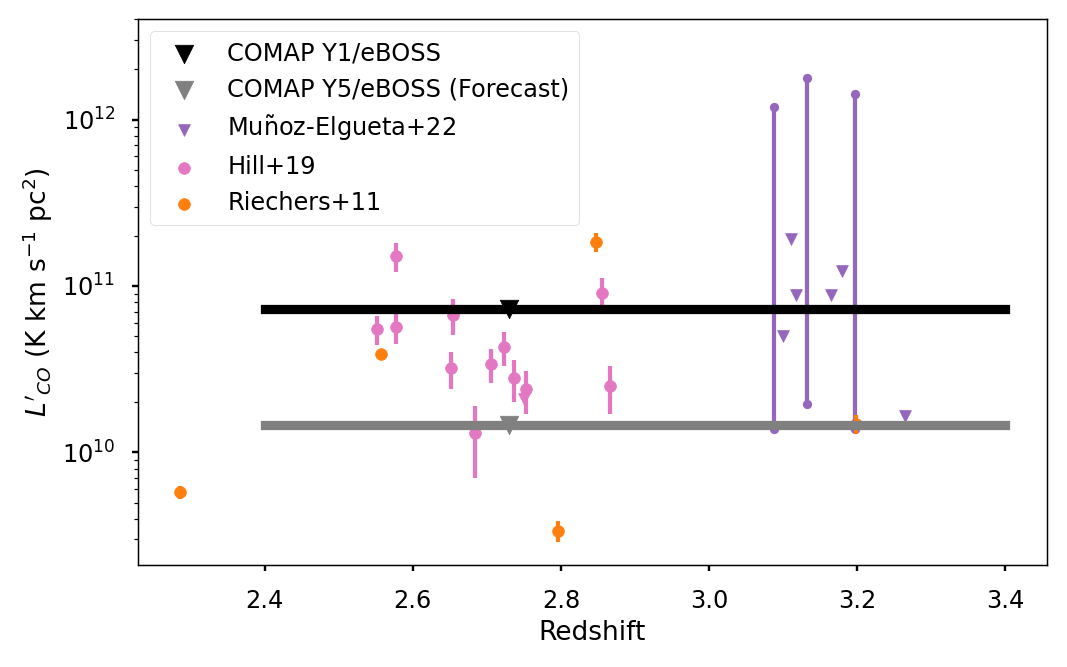
Figure 7: The COMAP/eBOSS 95% upper limit on $L^{\prime}_{\mathrm{CO}}$ (the black bar), plotted against quasars detected individually in CO from Riechers et al. (2011), Hill et al. (2019), and Muñoz-Elgueta et al. (2022). The extent of the COMAP/eBOSS bar indicates the redshift range to which COMAP is sensitive, and the marker is located at the mean redshift of the eBOSS objects on which we stack. A forecast for the stack sensitivity at the end of the full COMAP Pathfinder Survey is plotted in gray (see §4.2).

5.1 CO in Quasars

The response of the molecular gas in quasar host galaxies to the extremely active SMBH at their centers is likely extremely complicated, especially at cosmic noon. The abundances of both quasars and gas-rich, sub-mm-bright galaxies (SMGs) seem to peak during this epoch, suggesting a link between the two (Simpson et al., 2012). Indeed, both theoretical and observational arguments have suggested that the SMBH activity driving quasars is triggered from normal SMGs by mergers rich in cold and cool gas (Sanders et al., 1988; Hopkins et al., 2008; Brusa et al., 2018; Herrera-Camus et al., 2020; Bischetti et al., 2021), suggesting that, at least in their initial phases, quasars should be extremely rich in cold gas.

Whether that cold gas survives the subsequent barrage of heat and pressure from its central SMBH, however, is still uncertain. SMG studies of molecular gas have shown that the presence of an AGN does not seem to significantly affect the gas properties of its host (Bothwell et al., 2013; Banerji et al., 2017), and observed gas masses in quasars themselves follow typical SMG values closely (Hill et al., 2019), but other observations have shown that CO Spectral-Line Energy Distributions (SLEDs) in quasar hosts tend towards higher excitation states than normal (e.g., Brusa et al., 2018). At least for the purposes of COMAP, which measures the lowest CO excitation state, this would read as damped CO emission in quasar hosts. Additionally, many separate quasar studies have observed large scale outflows of all gas phases from the host galaxy, although a large fraction of this gas may remain in the molecular phase, and thus be observable with COMAP.

If we make the assumption that quasars are indeed CO-bright, meaning much of the CO luminosity contributing to the LIM maps at the quasar positions comes from the quasars themselves, then the upper limit on $L^{\prime}_{\mathrm{CO}}$ determined from our COMAP/eBOSS stack is very intuitive – it becomes a direct upper limit on the average CO line luminosity of the 282 eBOSS quasars included in the stack. This $L^{\prime}_{\mathrm{CO}}$ value is shown in Figure 7, plotted against other measures of quasar line luminosity in a similar redshift range, for comparison. These include the sample of 13 QSOs from KBSS, detected in CO(3-2) with NOEMA by Hill et al. (2019); the sample of 9 objects from the QSO MUSEUM, surveyed with APEX in CO(6-5) and CO(7-6) by Muñoz-Elgueta et al. (2022); and the sample of 5 QSOs detected in CO(1-0) by Riechers et al. (2011) using the Extended Very Large Array and the Green Bank Telescope.

The Hill et al. (2019) CO(3-2) measurements are converted into CO(1-0) line luminosities using the conversion factor $L^{\prime}_{\mathrm{CO(3-2)}}/L^{\prime}_{\mathrm{CO(1-0)}}=0.97\pm 0.19$ from Carilli & Walter (2013). In several cases, a single KBSS object was found to be associated with two different CO sources slightly offset on-sky. For each of these objects, we sum both CO sources together to obtain the plotted $L^{\prime}_{\mathrm{CO}}$ value, as both sources would fall well into the COMAP beam. Muñoz-Elgueta et al. (2022) converted their higher-$J$ CO measurements into molecular gas masses directly, by fitting to CO SLEDs, incorporating also the [CI] luminosity. In order to determine CO(1-0) line luminosities associated with the objects, we extrapolate their calculated $M_{\mathrm{H_{2}}}$ values to $L^{\prime}_{\mathrm{CO}}$ values using the Milky-Way $\alpha_{\mathrm{CO}}$ conversion factor of 3.6 M_⊙ ($\mathrm{K\ km\ s^{-1}\ pc^{-2}}$)^-1 (Bolatto et al., 2013), for consistency with our own previous analyses. These objects are mostly nondetections, and the SLED fitting returned a range of $M_{\mathrm{H_{2}}}$ values, so these ranges are what we plot in Figure 7. Riechers et al. (2011) report CO(1-0) line luminosities directly.

Figure 7 shows that the COMAP/eBOSS stacking upper limit is already comparable with the line luminosities of (the brightest) individually surveyed quasars in its redshift range, even using only the first season of COMAP data. In several cases, the COMAP value is actually a stricter limit, particularly for the APEX objects (Muñoz-Elgueta et al., 2022). This illustrates a powerful potential application for LIM – directly detecting CO in individual objects becomes prohibitively expensive very quickly at these redshifts. The 9 APEX quasars required $>130$ hours of observations per CO line with the APEX 12-m telescope, and, even then, five of the objects were not detected, despite targeting the higher-$J$ transitions that may be more prevelant in quasars. Similarly, Hill et al. (2019) required 2–5 hours of NOEMA time for each of their 13 CO(3-2) observations, and Riechers et al. (2011) used 25 hours of extended VLA time and 14.7 hours of GBT time to detect 5 objects in CO(1-0). While resolved observations of individual objects are obviously important for characterization of the behaviour of CO in quasars, a statistically-significant survey would require integration times that are not practical on high-demand community instruments.

Furthermore, while only an average value, and subject to the assumptions discussed above, our forecasted sensitivity to CO luminosity from a stack on the same 282 eBOSS quasars of the full five-year COMAP Pathfinder survey falls below the mean luminosity of the individually-detected quasars in Figure 7. We will therefore likely be able to tell with COMAP Y5 if these three samples are representative of the eBOSS quasar population as a whole. If we are able to constrain the $L^{\prime}_{\mathrm{CO}}$ of eBOSS quasars to this degree, it will provide significant insight into the complex feedback cycles present in quasars, and thus into star formation processes as a whole at cosmic noon.

5.2 Cosmic Molecular Gas Density

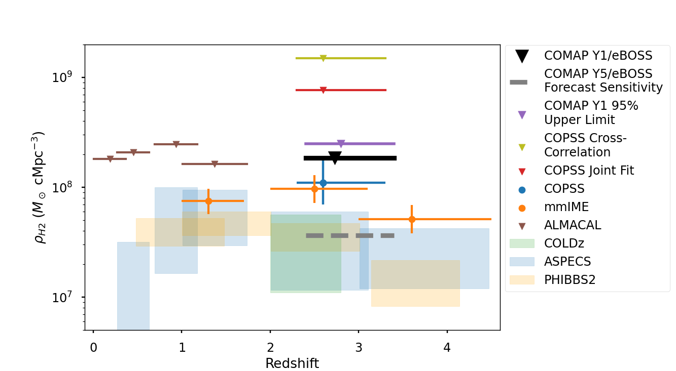
Figure 8: The upper limit on the average molecular gas density determined from the COMAP/eBOSS stack (black line), compared to other $\rho_{\mathrm{H_{2}}}$ measurements made using different survey techniques. The upper limit from the COMAP Season 1 power spectrum analysis is shown in purple. Also shown is the COPSS LIM survey’s measured value (Keating et al., 2016), as well as upper limits from COPSS joint analyses with galaxy surveys (Keenan et al., 2022). Shaded boxes are measurements made by large-scale traditional surveys COLDz (Riechers et al., 2019), ASPECS (González-López et al., 2019), and PHIBSS2 (Lenkić et al., 2020). We show the forecast $2\sigma$ sensitivity level of the five-year COMAP survey stacked on eBOSS as a grey upper limit.

The assumption that quasars trace large-scale structure is much better-supported than the assumption that quasars are CO-bright, as it follows from hierarchical structure formation. SMBH mass and galaxy mass have been shown several times to be correlated, meaning quasars will preferentially be found in massive galaxies that are likely to be at the center of large dark-matter halos (e.g., Gebhardt et al., 2000; Hopkins et al., 2008). This argument is additionally supported by clustering measurements of both BOSS and SDSS Stripe 82 quasars (White et al., 2012; Timlin et al., 2018), as well as observations of the individual objects shown in Figure 7: a quarter of the H19 objects, for example, have nearby CO-bright companions (also Banerji et al., 2017, 2018; Decarli et al., 2021; Bischetti et al., 2021). The argument that quasars require major mergers to ignite also necessitates at least one nearby massive galaxy in their recent past.

In the limit of this assumption, where the quasar host itself is contributing negligibly to a local overdensity of CO emission, we can use the stack’s upper limit on $T_{\mathrm{b}}$ to calculate the average molecular gas density $\rho_{\mathrm{H_{2}}}$ in bright regions at the COMAP redshifts. As the stack is only sensitive to a single, $\sim 9$ (comoving) Mpc spatial scale (the size of our chosen aperture), this value is most similar to a random ‘shot’ power component of the $\rho_{\mathrm{H_{2}}}$ determined from a power spectrum analysis. We plot this value in Figure 8, alongside several other measurements of the same value made using a variety of techniques, including COMAP’s own auto-spectrum based early science constraint (Chung et al., 2022). These other measurements include:

• COPSS (Keating et al., 2016), a LIM survey, targeting the same CO(1-0) transition as COMAP. COPSS used the Sunyaev-Zeldovich Array, and is subject to interferometric insensitivity to large scales. The $\rho_{\mathrm{H_{2}}}$ value from COPSS is thus based mainly on the shot-noise component of the CO power spectrum, converted to a molecular gas density using the Milky-Way $\alpha_{\mathrm{CO}}$ value of 3.6 M_⊙ (K km s^-1 pc^-2)^-1 (the same value we adopt in this work). Two other COPSS-determined values (Keenan et al., 2022) are plotted, both determined using joint analyses combining COPSS data with (after correcting for primary beam weighting) 145 spectroscopically-confirmed cataloged galaxies. Keenan et al. (2022) cross-correlated the COPSS data with a data cube obtained by gridding the catalog objects in 3D space (yielding one limit on $\rho_{\mathrm{H_{2}}}$) and fit the resulting cross-power spectrum jointly with both the auto-power spectrum of COPSS alone and the galaxy-galaxy power spectrum of their galaxy catalog (yielding a second $\rho_{\mathrm{H_{2}}}$ limit).

• ALMACAL (Klitsch et al., 2019) used archival ALMA calibrators as background sources to search blindly for CO absorption lines. As these calibrator sources must be observed frequently, ALMACAL boasts $>1500$ hours of observations on a community instrument over a wide enough area to not be limited by cosmic variance. However, these calibrators do not extend past $z\sim 2$.

• The Millimeter-wave Intensity Mapping Experiment (mmIME) used a combination of archival and targeted ALMA and Atacama Compact Array (ACA) observations at frequencies tracing multiple CO transitions (Keating et al., 2020). As with COPSS, these constraints are primarily constraints on the spectral shot power.

• Finally, the shaded boxes in Figure 8 correspond to $\rho_{\mathrm{H_{2}}}$ measurements made using traditional (i.e., resolved and targeted) galaxy surveys. These include ASPECS (Uzgil et al., 2019; González-López et al., 2019) and PHIBBS2 (Lenkić et al., 2020), each tracing multiple CO rotational transitions, as well as COLDz (Riechers et al., 2019), which traces exclusively CO(1-0) at $z\sim 3$. While each of these traditional surveys provide $\rho_{\mathrm{H_{2}}}$ values that seem like much better constraints than any of the LIM-based numbers, they cover much smaller survey volumes and are thus extremely subject to cosmic varience effects. Additionally, as traditional surveys, they are insensitive to any emission below their detection limits, and so will miss any contribution to the total gas density from fainter objects, likely underestimating the total gas density.

Clearly, these $\rho_{\mathrm{H_{2}}}$ measurements were made using a diverse range of different techniques, so some of the scatter in Figure 8 can be attributed simply to the biases associated with each strategy. There is also likely additional scatter present due to variations in the CO-to-H₂ ratio, both astrophysically and in the conversion factor $\alpha_{\mathrm{CO}}$ chosen for each analysis, as well as the relative intensity of the different CO line transitions, which will also change based on environment.

In our case, while we are indeed subject to the assumptions associated with our choice of $\alpha_{\mathrm{CO}}$ and the bias of CO emission as a galaxy tracer, we are also only investigating the regions of space associated with eBOSS quasars, so the stacking analysis necessarily introduces a secondary bias factor. Due to this additional bias, the $\rho_{\mathrm{H_{2}}}$ value from the eBOSS stack is more similar to a cross-correlation analysis, such as the early WMAP cross-correlations with SDSS and BOSS quasars (Pullen & Hirata, 2013; Pullen et al., 2013). Unlike these cross-correlation analyses, the stack’s $\rho_{\mathrm{H_{2}}}$ value is only sensitive to a single spatial scale (the scale of the 3D stack aperture, $\sim 9$ cMpc). As discussed above, regions of this size surrounding quasars are likely to be more dense than the universe as a whole, biasing the stacked $\rho_{\mathrm{H_{2}}}$ value upwards. This is again acceptable in the context of an upper limit – even after a detection is made, we expect the stack $\rho_{\mathrm{H_{2}}}$ value to be an upper limit on the overall H₂ density of the universe.

Even with these caveats, however, our predicted value is comparable to the values returned from the different COPSS joint analyses, reinforcing the viability of stacking as a LIM tool introduced by Keenan et al. (2022). More promising is our forecast sensitivity for the COMAP Y5/eBOSS stack, which actually falls into the regions reported by traditional galaxy surveys. As these galaxy-survey values are likely underestimates of the actual cosmic H₂ density, our stacking analysis should detect emission from even very pessimistic models of cosmic CO, provided our forecasts hold true. As we already predict that our autocorrelation analysis will allow us to discriminate between CO models by COMAP Y5 (Chung et al., 2022), stacking will provide another valuable tool in characterizing the amount and properties of molecular gas emission at cosmic noon.

Additionally, quasar catalogs are far from the only spectroscopic information available on astrophysical objects at our redshifts. As discussed in §4.2, increasing the number of objects in our galaxy catalog will increase the sensitivity of our stack, but introducing new objects detected using different tracers will also provide new opportunities for analysis. It will be very interesting to compare, for example, the CO properties of the LAEs in the HETDEX survey (Gebhardt et al., 2021) to the CO properties of the eBOSS quasars. Galaxy evolution is an inherently multitracer problem, so there will be significant analysis benefits to collating as many different surveys (whether traditional resolved surveys or LIM experiments) of the same region of space as possible. As the LIM field progresses, there will be more and more opportunities to do so.

6 Summary and Conclusions

By stacking CO line-intensity maps from COMAP’s first year of science operations on the 3D positions of quasars from the SDSS eBOSS survey, we have obtained a new upper limit on the cosmic abundance of molecular hydrogen gas. We describe the methodology behind the stack in detail, including the COMAP RMS-based weighting scheme we use when coadding and the bootstrapped error analysis technique we use to quantify uncertainties. We use the stack to search additionally for interloper emission from foreground galaxies in four molecular lines, finding no evidence of a detection in any case. We can interpret our stacked upper limit as a constraint on the CO emission from either the cataloged quasars themselves, or the regions of the universe surrounding those quasars. Likely, the most realistic interpretation is some combination of both cases. Additionally, we forecast stacking results for the full five-year COMAP Pathfinder survey.

Under the assumption that any potential signal in the stack is CO emission from the eBOSS quasars themselves, we treat our measurement as the average CO luminosity of these objects. We compare this average luminosity to resolved CO measurements of quasars in the COMAP redshift range, and find that our upper limit already probes CO luminosities fainter than those of the brightest objects observed to date. The quasar studies to which we compare typically required hours of observations using large community facilities to detect CO in only a handful of objects. Determining the CO properties of a large sample of objects such as our subset of the eBOSS catalog would thus be prohibitively expensive through traditional means. LIM stacks, therefore, could potentially be extremely useful as a tool for studying large samples of high-redshift galaxies and quasars.

Conversely, if we assume that the eBOSS quasars do not significantly contribute to the integrated CO emission of their surroundings, the stacked flux measurement can be converted to a measurement of the cosmic molecular gas density. While we compare this value directly to other $\rho_{\mathrm{H_{2}}}$ measurements from various sources, its interpretation is somewhat more complicated, as the molecular gas density in the regions traced by the stack depends heavily on the bias of the cataloged quasars towards large-scale structure. Additionally, the stack probes only a single spatial scale, unlike the more conventional power spectrum-based LIM measurements. These differences make stacking an excellent complement to other LIM analyses.

We propose, therefore, that stacking analyses with existing galaxy catalogs are a promising addition to the LIM analysis toolbox, especially when using LIM to approach as complex and multi-tracer a problem as galaxy evolution. To take full advantage of their potential benefits, stacking analyses should be performed on catalogs using as many different galaxy tracers as possible, to probe this phase space more fully. We aim to investigate stacking as a galaxy analysis tool more fully in future works, including by stacking on the extensive HETDEX catalog of Lyman-$\alpha$ emitters (Gebhardt et al., 2021).

7 Acknowledgements

This material is based upon work supported by the National Science Foundation under Grant Nos. 1518282, 1517108, 1517598, 1517288, 1910999 and 2206834; by the Keck Institute for Space Studies under “The First Billion Years: A Technical Development Program for Spectral Line Observations”; and by a seed grant from the Kavli Institute for Particle Astrophysics and Cosmology.

DD acknowledges support from NSF Award 2206834. KC acknowledges support from NSF Awards 1518282, 1910999 and 2206834. PCB is supported by the James Arthur Postdoctoral Fellowship. DC is supported by a CITA/Dunlap Institute postdoctoral fellowship. The Dunlap Institute is funded through an endowment established by the David Dunlap family and the University of Toronto. HI, HKE, and IW acknowledge support from the Research Council of Norway through grant 251328. JG acknowledges support from the Keck Institute for Space Science, NSF AST-1517108 and University of Miami and Hugh Medrano for assistance with cryostat design. JK is supported by a Robert A. Millikan Fellowship from Caltech. HP’s research is supported by the Swiss National Science Foundation via Ambizione Grant PZ00P2_179934.

This research made use of the SDSS-IV eBOSS survey. Funding for the Sloan Digital Sky Survey IV has been provided by the Alfred P. Sloan Foundation, the U.S. Department of Energy Office of Science, and the Participating Institutions.

SDSS-IV acknowledges support and resources from the Center for High Performance Computing at the University of Utah. The SDSS website is www.sdss4.org.

SDSS-IV is managed by the Astrophysical Research Consortium for the Participating Institutions of the SDSS Collaboration including the Brazilian Participation Group, the Carnegie Institution for Science, Carnegie Mellon University, Center for Astrophysics — Harvard & Smithsonian, the Chilean Participation Group, the French Participation Group, Instituto de Astrofísica de Canarias, The Johns Hopkins University, Kavli Institute for the Physics and Mathematics of the Universe (IPMU) / University of Tokyo, the Korean Participation Group, Lawrence Berkeley National Laboratory, Leibniz Institut für Astrophysik Potsdam (AIP), Max-Planck-Institut für Astronomie (MPIA Heidelberg), Max-Planck-Institut für Astrophysik (MPA Garching), Max-Planck-Institut für Extraterrestrische Physik (MPE), National Astronomical Observatories of China, New Mexico State University, New York University, University of Notre Dame, Observatário Nacional / MCTI, The Ohio State University, Pennsylvania State University, Shanghai Astronomical Observatory, United Kingdom Participation Group, Universidad Nacional Autónoma de México, University of Arizona, University of Colorado Boulder, University of Oxford, University of Portsmouth, University of Utah, University of Virginia, University of Washington, University of Wisconsin, Vanderbilt University, and Yale University.

This research made use of NASA’s Astrophysics Data System Bibliographic Services. For the purpose of open access, the authors have applied a Creative Commons Attribution (CC BY) licence to any Author Accepted Manuscript version arising from this submission.

Appendix A Foreground Stacks

A.1 ¹²CO(1-0) Offset by Quasar Value

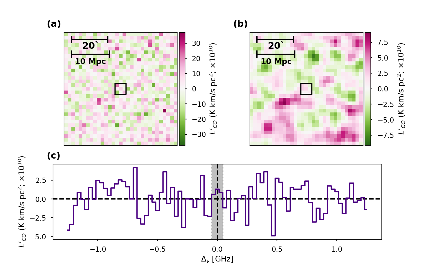
Figure 9: The 3D stack performed on the eBOSS catalog using the ¹²CO(1-0) emission wavelength offset by the frequency offset found in individually-detected quasars (see §4.1). See Figure 4 for panel descriptions.

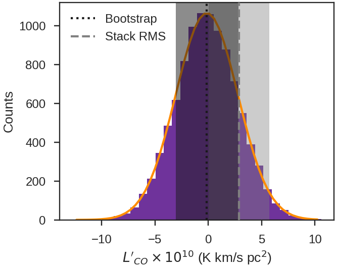
Figure 10: The bootstrapped uncertainties in $L^{\prime}_{\mathrm{CO}}$ for the offset ¹²CO(1-0) stack (see Figure 5.

A.2 HCN(1-0)

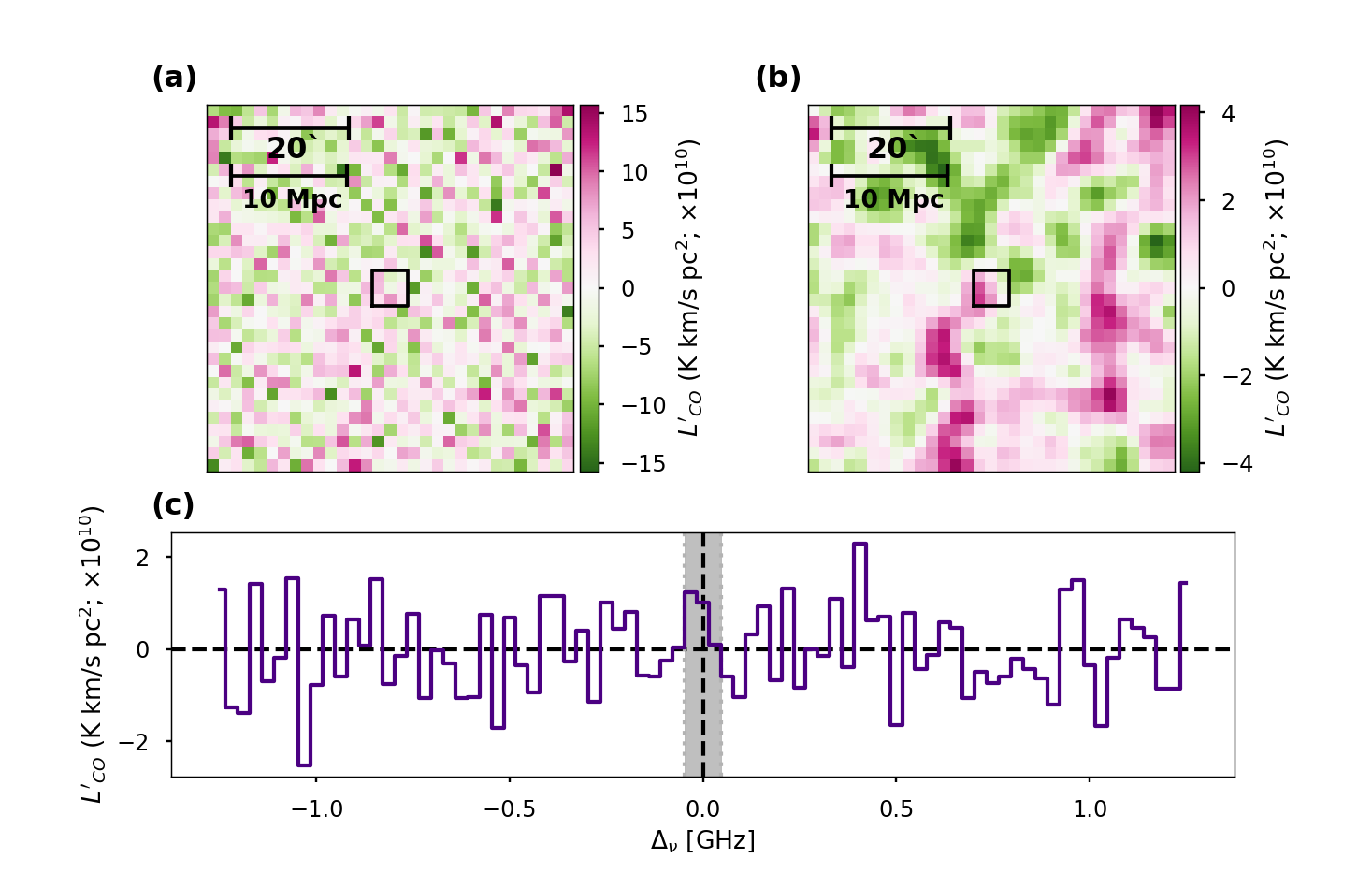
Figure 11: The 3D stack performed on the eBOSS catalog using the HCN(1-0) emission wavelength. See Figure 4 for panel descriptions.

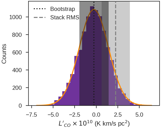
Figure 12: The bootstrapped uncertainties in $L^{\prime}_{\mathrm{CO}}$ for the HCN(1-0) stack (see Figure 5).

A.3 CS(2-1)

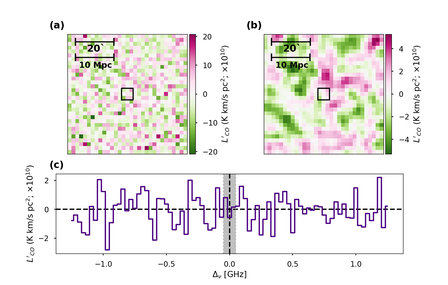
Figure 13: The 3D stack performed on the eBOSS catalog using the CS(2-1) emission wavelength. See Figure 4 for panel descriptions.

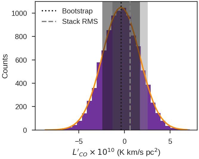
Figure 14: The bootstrapped uncertainties in $L^{\prime}_{\mathrm{CO}}$ for the CS(2-1) stack (see Figure 5).

A.4 ¹³CO(1-0)

Figure 15: The 3D stack performed on the eBOSS catalog using the ¹³CO(1-0) emission wavelength. See Figure 4 for panel descriptions.

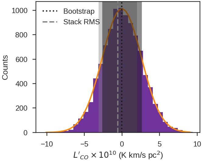
Figure 16: The bootstrapped uncertainties in $L^{\prime}_{\mathrm{CO}}$ for the ¹³CO(1-0) stack (see Figure 5).

A.5 CN^-(1-0)

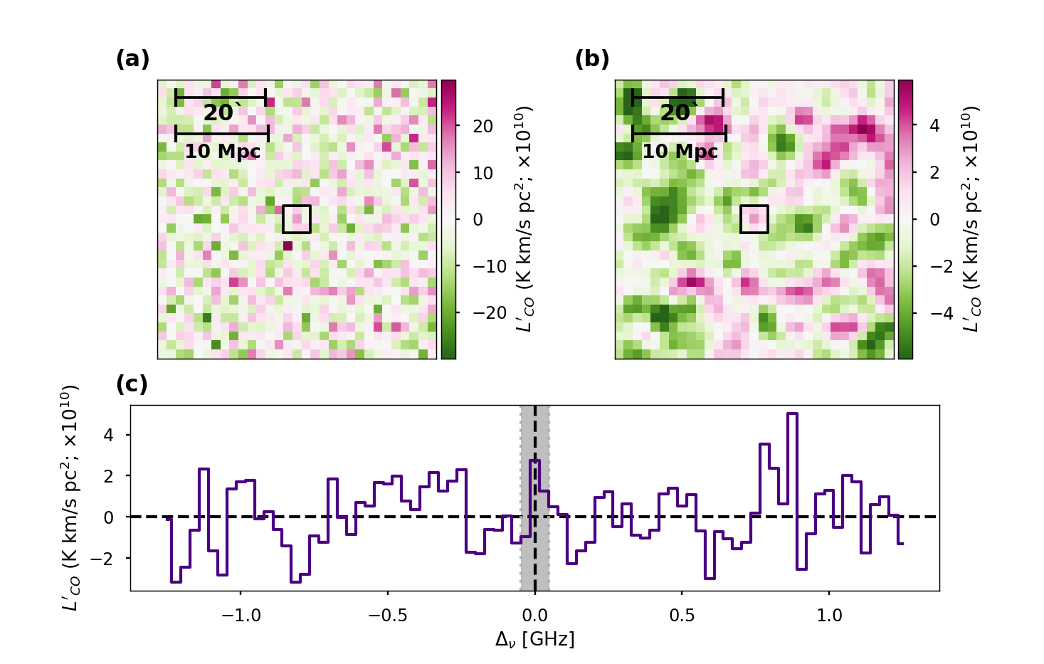
Figure 17: The 3D stack performed on the eBOSS catalog using the CN^-(1-0) emission wavelength. See Figure 4 for panel descriptions.

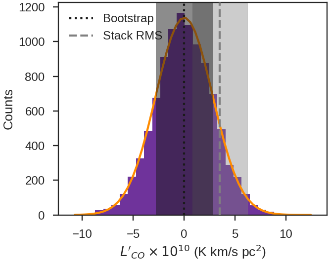
Figure 18: The bootstrapped uncertainties in $L^{\prime}_{\mathrm{CO}}$ for the CN^-(1-0) stack (see Figure 5).

References

- Abdurashidova et al. (2022) Abdurashidova, Z., Aguirre, J. E., Alexander, P., et al. 2022, ApJ, 925, 221, doi: 10.3847/1538-4357/ac1c78
- Ahumada et al. (2020) Ahumada, R., Prieto, C. A., Almeida, A., et al. 2020, ApJS, 249, 3
- Astropy Collaboration et al. (2013) Astropy Collaboration, Robitaille, T. P., Tollerud, E. J., et al. 2013, A&A, 558, A33, doi: 10.1051/0004-6361/201322068
- Astropy Collaboration et al. (2018) Astropy Collaboration, Price-Whelan, A. M., Sipőcz, B. M., et al. 2018, AJ, 156, 123, doi: 10.3847/1538-3881/aabc4f
- Banerji et al. (2017) Banerji, M., Carilli, C. L., Jones, G., et al. 2017, MNRAS, 465, 4390, doi: 10.1093/mnras/stw3019
- Banerji et al. (2018) Banerji, M., Jones, G. C., Wagg, J., et al. 2018, MNRAS, 479, 1154, doi: 10.1093/mnras/sty1443
- Bautista et al. (2017) Bautista, J. E., Busca, N. G., Guy, J., et al. 2017, A&A, 603, A12, doi: 10.1051/0004-6361/201730533
- Belitsky et al. (2018) Belitsky, V., Lapkin, I., Fredrixon, M., et al. 2018, A&A, 612, A23, doi: 10.1051/0004-6361/20173145810.48550/arXiv.1712.07396
- Bischetti et al. (2021) Bischetti, M., Feruglio, C., Piconcelli, E., et al. 2021, A&A, 645, A33, doi: 10.1051/0004-6361/202039057
- Bolatto et al. (2013) Bolatto, A. D., Wolfire, M., & Leroy, A. K. 2013, ARA&A, 51, 207, doi: 10.1146/annurev-astro-082812-140944
- Bolton et al. (2012) Bolton, A. S., Schlegel, D. J., Aubourg, É., et al. 2012, AJ, 144, 144, doi: 10.1088/0004-6256/144/5/144
- Bothwell et al. (2013) Bothwell, M. S., Smail, I., Chapman, S. C., et al. 2013, MNRAS, 429, 3047, doi: 10.1093/mnras/sts562
- Breysse & Alexandroff (2019) Breysse, P. C., & Alexandroff, R. M. 2019, MNRAS, 490, 260–273, doi: 10.1093/mnras/stz2534
- Brusa et al. (2018) Brusa, M., Cresci, G., Daddi, E., et al. 2018, A&A, 612, A29, doi: 10.1051/0004-6361/201731641
- Carilli & Walter (2013) Carilli, C., & Walter, F. 2013, Annual Review of Astronomy and Astrophysics, 51, 105, doi: 10.1146/annurev-astro-082812-140953
- Chenu et al. (2016) Chenu, J.-Y., Navarrini, A., Bortolotti, Y., et al. 2016, IEEE Transactions on Terahertz Science and Technology, 6, 223, doi: 10.1109/TTHZ.2016.2525762
- Chung et al. (2019) Chung, D. T., Viero, M. P., Church, S. E., et al. 2019, ApJ, 872, 186, doi: 10.3847/1538-4357/ab0027
- Chung et al. (2021) Chung, D. T., Breysse, P. C., Ihle, H. T., et al. 2021, ApJ, 923, 188, doi: 10.3847/1538-4357/ac2a35
- Chung et al. (2022) Chung, D. T., Breysse, P. C., Cleary, K. A., et al. 2022, ApJ, 933, 186, doi: 10.3847/1538-4357/ac63c7
- Cleary et al. (2022) Cleary, K. A., Borowska, J., Breysse, P. C., et al. 2022, ApJ, 933, 182, doi: 10.3847/1538-4357/ac63cc
- Dawson et al. (2013) Dawson, K. S., Schlegel, D. J., Ahn, C. P., et al. 2013, AJ, 145, 10, doi: 10.1088/0004-6256/145/1/10
- Dawson et al. (2016) Dawson, K. S., Kneib, J.-P., Percival, W. J., et al. 2016, ApJ, 151, 44, doi: 10.3847/0004-6256/151/2/44
- Decarli et al. (2021) Decarli, R., Arrigoni-Battaia, F., Hennawi, J. F., et al. 2021, A&A, 645, L3, doi: 10.1051/0004-6361/202039814
- Foss et al. (2022) Foss, M. K., Ihle, H. T., Borowska, J., et al. 2022, ApJ, 933, 184, doi: 10.3847/1538-4357/ac63ca
- Gebhardt et al. (2000) Gebhardt, K., Bender, R., Bower, G., et al. 2000, ApJ, 539, L13, doi: 10.1086/312840
- Gebhardt et al. (2021) Gebhardt, K., Mentuch Cooper, E., Ciardullo, R., et al. 2021, ApJ, 923, 217, doi: 10.3847/1538-4357/ac2e03
- González-López et al. (2019) González-López, J., Decarli, R., Pavesi, R., et al. 2019, ApJ, 882, 139, doi: 10.3847/1538-4357/ab3105
- Gunn et al. (2006) Gunn, J. E., Siegmund, W. A., Mannery, E. J., et al. 2006, AJ, 131, 2332, doi: 10.1086/500975
- Herrera-Camus et al. (2020) Herrera-Camus, R., Janssen, A., Sturm, E., et al. 2020, A&A, 635, A47, doi: 10.1051/0004-6361/201936434
- Hill et al. (2019) Hill, R., Chapman, S. C., Scott, D., et al. 2019, MNRAS, 485, 753, doi: 10.1093/mnras/stz429
- Hinshaw et al. (2013) Hinshaw, G., Larson, D., Komatsu, E., et al. 2013, ApJS, 208, 19, doi: 10.1088/0067-0049/208/2/19
- Hopkins et al. (2008) Hopkins, P. F., Hernquist, L., Cox, T. J., & Kereš, D. 2008, ApJS, 175, 356, doi: 10.1086/524362
- Hunter (2007) Hunter, J. D. 2007, Computing in Science & Engineering, 9, 90, doi: 10.1109/MCSE.2007.55
- Ihle et al. (2022) Ihle, H. T., Borowska, J., Cleary, K. A., et al. 2022, ApJ, 933, 185, doi: 10.3847/1538-4357/ac63c5
- Jolly et al. (2021) Jolly, J.-B., Knudsen, K., Laporte, N., et al. 2021, A&A, 652, A128, doi: 10.1051/0004-6361/202140878
- Keating et al. (2020) Keating, G. K., Marrone, D. P., Bower, G. C., & Keenan, R. P. 2020, ApJ, 901, 141, doi: 10.3847/1538-4357/abb08e
- Keating et al. (2016) Keating, G. K., Marrone, D. P., Bower, G. C., et al. 2016, ApJ, 830, 34
- Keenan et al. (2022) Keenan, R. P., Keating, G. K., & Marrone, D. P. 2022, ApJ, 927, 161, doi: 10.3847/1538-4357/ac4888
- Klitsch et al. (2019) Klitsch, A., Péroux, C., Zwaan, M. A., et al. 2019, MNRAS, 490, 1220, doi: 10.1093/mnras/stz2660
- Kovetz et al. (2019) Kovetz, E., Breysse, P. C., Lidz, A., et al. 2019, BAAS, 51, 101. https://arxiv.org/abs/1903.04496
- Lamb et al. (2022) Lamb, J. W., Cleary, K. A., Woody, D. P., et al. 2022, ApJ, 933, 183, doi: 10.3847/1538-4357/ac63c6
- Lenkić et al. (2020) Lenkić, L., Bolatto, A. D., Förster Schreiber, N. M., et al. 2020, AJ, 159, 190, doi: 10.3847/1538-3881/ab7458
- Lujan Niemeyer et al. (2022) Lujan Niemeyer, M., Komatsu, E., Byrohl, C., et al. 2022, ApJ, 929, 90, doi: 10.3847/1538-4357/ac5cb8
- Lyke et al. (2020) Lyke, B. W., Higley, A. N., McLane, J. N., et al. 2020, ApJS, 250, 8, doi: 10.3847/1538-4365/aba623
- Muñoz-Elgueta et al. (2022) Muñoz-Elgueta, N., Arrigoni Battaia, F., Kauffmann, G., et al. 2022, MNRAS, 511, 1462, doi: 10.1093/mnras/stac041
- Paul et al. (2023) Paul, S., Santos, M. G., Chen, Z., & Wolz, L. 2023, arXiv e-prints, arXiv:2301.11943, doi: 10.48550/arXiv.2301.11943
- Pullen et al. (2013) Pullen, A. R., Chang, T.-C., Doré, O., & Lidz, A. 2013, ApJ, 768, 15, doi: 10.1088/0004-637X/768/1/15
- Pullen & Hirata (2013) Pullen, A. R., & Hirata, C. M. 2013, PASP, 125, 705, doi: 10.1086/671189
- Rennie et al. (2022) Rennie, T. J., Harper, S. E., Dickinson, C., et al. 2022, ApJ, 933, 187, doi: 10.3847/1538-4357/ac63c8
- Riechers et al. (2011) Riechers, D. A., Carilli, C. L., Maddalena, R. J., et al. 2011, ApJ, 739, L32, doi: 10.1088/2041-8205/739/1/L32
- Riechers et al. (2019) Riechers, D. A., Pavesi, R., Sharon, C. E., et al. 2019, ApJ, 872, 7, doi: 10.3847/1538-4357/aafc27
- Romano et al. (2022) Romano, M., Morselli, L., Cassata, P., et al. 2022, A&A, 660, A14, doi: 10.1051/0004-6361/202142265
- Sanders et al. (1988) Sanders, D. B., Soifer, B. T., Elias, J. H., Neugebauer, G., & Matthews, K. 1988, ApJ, 328, L35, doi: 10.1086/185155
- Silva et al. (2021) Silva, M. B., Baumschlager, B., Cleary, K. A., et al. 2021, arXiv e-prints, arXiv:2111.05354. https://arxiv.org/abs/2111.05354
- Simpson et al. (2012) Simpson, J. M., Smail, I., Swinbank, A. M., et al. 2012, MNRAS, 426, 3201, doi: 10.1111/j.1365-2966.2012.21941.x
- Sinigaglia et al. (2022) Sinigaglia, F., Elson, E., Rodighiero, G., & Vaccari, M. 2022, MNRAS, 514, 4205, doi: 10.1093/mnras/stac1584
- Smee et al. (2013) Smee, S. A., Gunn, J. E., Uomoto, A., et al. 2013, AJ, 146, 32, doi: 10.1088/0004-6256/146/2/32
- Solomon et al. (1997) Solomon, P. M., Downes, D., Radford, S. J. E., & Barrett, J. W. 1997, ApJ, 478, 144, doi: 10.1086/303765
- Stanley et al. (2019) Stanley, F., Jolly, J. B., König, S., & Knudsen, K. K. 2019, A&A, 631, A78, doi: 10.1051/0004-6361/201834530
- Stein et al. (2019) Stein, G., Alvarez, M. A., & Bond, J. R. 2019, MNRAS, 483, 2236, doi: 10.1093/mnras/sty3226
- Timlin et al. (2018) Timlin, J. D., Ross, N. P., Richards, G. T., et al. 2018, ApJ, 859, 20, doi: 10.3847/1538-4357/aab9ac
- Uzgil et al. (2019) Uzgil, B. D., Carilli, C., Lidz, A., et al. 2019, ApJ, 887, 37, doi: 10.3847/1538-4357/ab517f
- White et al. (2012) White, M., Myers, A. D., Ross, N. P., et al. 2012, MNRAS, 424, 933, doi: 10.1111/j.1365-2966.2012.21251.x