${\boldsymbol{\cal N}}$ = 2 SUSY & the Hexipentisteriruncicantitruncated 7-Simplex

                 Aleksander J. Cianciara^a,b, Zachary Coleman^,c,d,e,
S. James Gates, Jr.^f, Youngik (Tom) Lee^,g,h, and Ziyang Zhang^,g,h             

^aJoseph Henry Laboratories, Princeton University, Princeton, NJ 08544, USA,
^bInstitute for Advanced Study, Princeton, NJ 08540, USA,
^cPepperdine University, Natural Science Division, Malibu, CA 90263, USA,
^dMathematics Institute, University of Oxford, Oxford OX2 6GG, UK,
^e Department of Physics, University of Oxford, Oxford OX1 3PU, UK,
^fDepartment of Physics, University of Maryland,
College Park, MD 20742-4111, USA,
^gBrown University, Department of Physics,
182 Hope Street, Barus & Holley 545, Providence, RI 02912, USA,
^hBrown Center for Theoretical Physics,
340 Brook Street, Barus Hall, Providence, RI 02912, USA,

ABSTRACT

We study algorithms for recursively creating arbitrary $N$-extended ‘supermultiplets’ given minimal matrix representations of off-shell, $\cal N$ = 1 supermultiplet matrices. We observe connections between the color vertex problems in graph theory and the different supermultiplet sets locations in the permutahedron by using the concepts of truncation and chromatic number. The concept of ‘hopping operators’ is introduced, constructed, and then used to partition the $8!$ vertices of the permutahedron. We explicitly partition these into 5,040 octets constrained in locations on the permutahedron by a magic number rule. Boolean factors in this recursive construction are shown to obey a doubly even binary flip rule. Although these hopping operators do not generally constitute normal subgroups of the permutation group, we find that ‘ab-normal cosets’ exist where the same left- and right-hoppers appear as unordered sets. Finally, using computer simulations, we investigate the types of faces on higher-order permutahedron which may give rise to lower-order supermultiplets.

PACS: 11.30.Pb, 12.60.Jv
Keywords: supersymmetry, permutahedron, supermultiplet

1 Introduction

The question of how to create arbitrary 4D, $N$-extended supermultiplets (represented by matrices) starting from minimal 4D, $\cal N$ = 1 realizations began with  [?,?] and was one of the motivations for the DFGHILM collaboration. Later it was realized  [?] the matrices utilized could be interpreted as modified versions of adjacency matrices for a set of graphs given the names of “adinkras.” More recently  [?], it was shown that the permutahedron plays a role in the selection of supermultiplets, and that some faces of the permutahedron polytope related to a given value of $\cal N$ correspond to valid supermultiplets of a lower degree or extension  [?]. In other areas, it’s been shown that faces of polytopes may correspond to properties of effective field theories  [?]. The present connection between representations of supersymmetry and permutation polytopes hints at an underlying polytopic representation theory that may be responsible for generating all valid representations of supersymmetry. Similar work has been carried out examining the structure of viruses  [?], building off the idea of Watson and Crick that the crystallographic symmetry of viruses could be explained by the repeated use of just a few protein subunits (in the present paper we call these hopping operators)  [?].

The results in this work give an extension of the questions and results determined about the recursive construction of higher $N$-extended 1D, adinkra matrices from lower $N$-extended 1D, adinkra matrices in the works of  [?,?]. In this work similar questions and results are determined for the extension of adinkra matrices associated with 4D, $\cal N$ = 1 models expanded to adinkra matrices associated with 4D, $\cal N$ = 2 models.

1.1 A problem from the representation theory: at the foundation of 4-dimensional supersymmetry

In mathematics, the four color map conjecture dates back to 1852  [?], and apparently its extension to a major theorem was the first proven by means of computers and information technology  [?,?]. While at the time of the announcement in 1976 there was some controversy, by now there seems to be a general acceptance of the proof’s validity. For a number of years a program of IT use has been under development  [?,?,?,?,?] to explore problems at the mathematical foundations of supersymmetry. In particular, the work of  [?] showed the concept of “off-shell” 4D, $\cal N$ = 1 supersymmetry leading to the study of Coxeter Groups. This work demonstrated that there exists a direct sum partitioning of the totality of BC(4) matrix representations into six disjoint subsets of matrices representing Clifford Algebras. The permutation matrices are assigned as shown in Fig. 1 where each permutation matrix is indicated to belong to one of six (color-coded for convenience sake) subsets. Upon taking the absolute values of these BC(4) matrix representations, one is led to twenty-four matrices that provide a matrix representation of the permutation group of order four. The permutahedron is a well-known concept related to the study of permutation groups and all the members can properly be assigned using weak right Bruhat ordering  [?] to the appropriate location as shown in Fig. 3.

This naturally leads to the question of whether there is an invariant associated with the permutation group of order four that determines the assignments of the members of the subsets to the distinct patterns of locations in the permutahedron. This answer is yes. In the past , we have used the symbols ${\cal G}_{(1)}$, and ${\cal G}_{(2)}$ to denote maps from adinkra graphs to the real numbers. In this work, we define a new mapping operator that will be denoted by ${\cal G}_{(3)}$. Unlike the previous two mapping operations, this new one is defined by the decoration of the nodes of the permutahedron by sets of colored spheres.

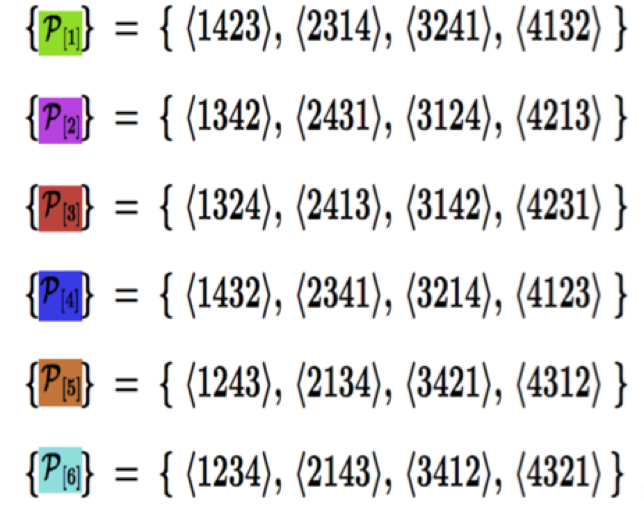
Figure 1: Permutation matrix assignments to subsets

The permutahedron is shown in Fig. 3, and the six subsets are shown in Fig. 3.

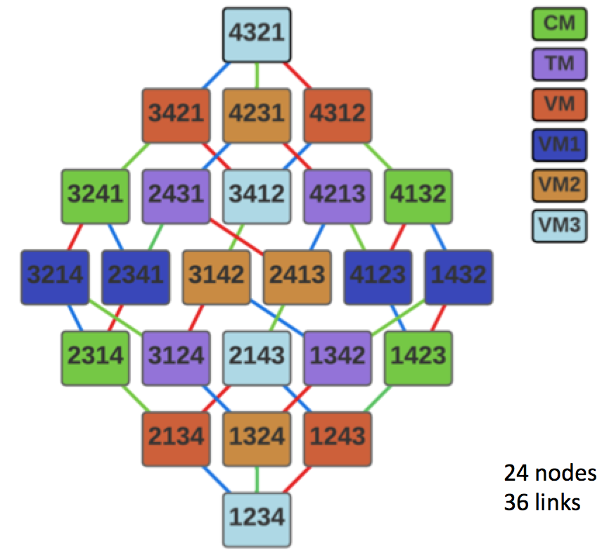
Figure 2: Permutahedron containing subset elements

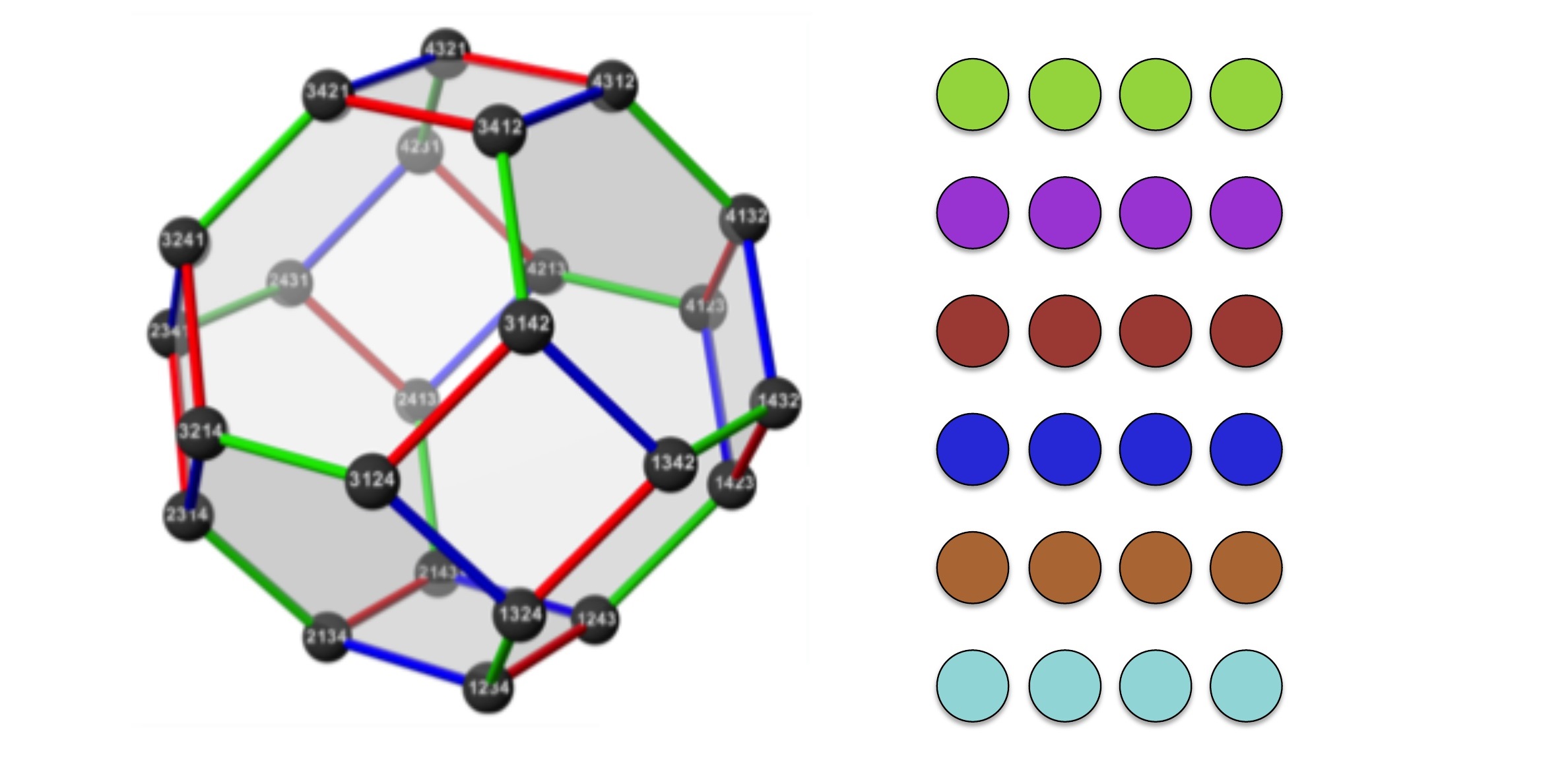
Figure 3: Permutahedron and subsets

The truncated octahedron is a well known Archimedean solid that contains 24 vertices as shown in Fig. 4. Let us consider the case where 24 spheres (as shown to the right in Fig. 3 are placed at vertices of the truncated octahedron, one sphere to each vertex to adorn the solid). However, the spheres are not all identical. Six disjoint sets each containing four spheres of the same color, are shown in Fig. 4. After placing all of the spheres at vertices, a particular sphere can be specified, and then the minimum number of edges traversed to go to the locations of the remaining three spheres of the same color can be noted and summed.

A problem to solve is how to place the 24 spheres at the vertices so that the sum described above is the same independent of the choice of color.

As one example of such a solution, it can be noted that the truncated octahedron possesses six faces that are squares. So a solution is obtained by choosing four spheres of the same color and placing them at the vertices of one of the square faces. Upon choosing one of these spheres as the fiducial one, there are two other spheres adjacent to it and connected by one edge. The remaining sphere is connected to this chosen sphere by two edges. Thus the sum of the numbers of edges connecting the chosen sphere to the other three is ${\cal G}{}_{(3)}$ = 1 + 1 + 2 = 4. As all the square faces are equivalent, the choice of which color of spheres over which to carry out this calculation is irrelevant.

An interesting question to entertain is whether there are other placements of the spheres which have the same property with respect to such an invariant and what is the numerical value for this invariant for these other placements.

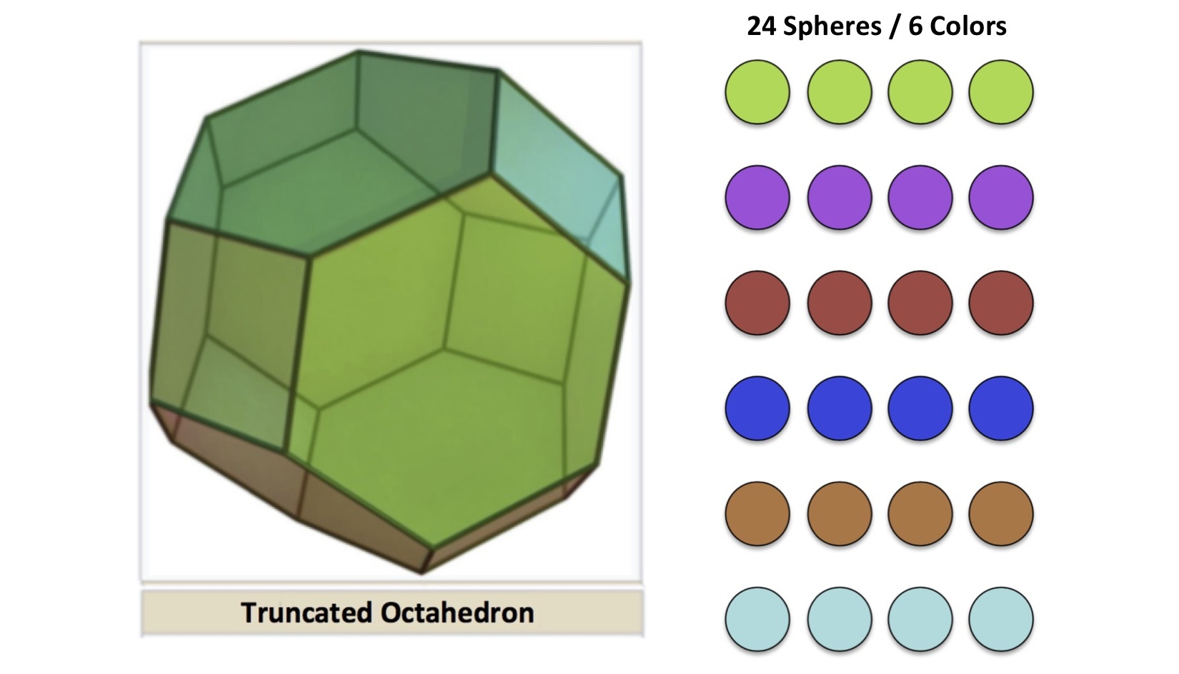
Figure 4: Twenty-four spheres with six different colors next to a truncated octahedron

There is a second such solution: it is the one obtained by using the image in Fig. 3 as a guide to all the positioning of the colored spheres. Carrying out the same calculation upon picking a fiducial sphere of any color leads to ${\cal G}{}_{(3)}$ = 2 + 4 + 6 = 12. Furthermore, this result is independent of the color of the spheres that are chosen. This choice of decoration is the one that is required to implement the disassociation of the Coxeter Group BC(4) matrices in six sets of matrices representing Clifford Algebras. We call ${\cal G}{}_{(3)}$ = 12 the “magic number” and will return to this in the remainder of the discussion.

The problem described above can be generalized to permutations groups of higher order. For the permutation group of order $8$, there will be $8!$ nodes and the number of distinct colors will be $8$. In this case, there are 191,520 faces, 141,120 edges, 40,320 nodes and 8 colors.

Moreover, the solution with ${\cal G}{}_{(3)}$ = 12 can be interpreted as a solution of a graph vertex coloring problem  [?]. The graph vertex coloring problem is defined as the process of coloring the nodes in such a way that no two nodes sharing a common edge of the graph have the same color. The smallest number of colors needed to color a graph $G$ is called the chromatic number, denoted as $\chi(G)$  [?]. It can be seen that our first proposed solution with ${\cal G}{}_{(3)}$ = 4 is not a solution of the graph vertex coloring problem.

Then one question we can ask is whether any geometric method exists to construct the second coloring solution suggested above. In order to do this, first let us define the “restricted chromatic number" under the stronger restrictions on graph coloring, as the smallest number of colors needed to color for an arbitrary graph $G$ that ${\cal G}{}_{(3)}$ has a constant value and independent of the choice of color. Then one can show that the restricted chromatic number of the permutahedron is 2 as in Fig. 5. Secondly, after coloring the vertices of the permutahedron with two colors (metallic gold and silver), we can transform the 12 metallic gold vertices of the permutahedron onto the cuboctahedron as on the right in Fig. 5. (We can repeat the same process with all of the silver vertices.)

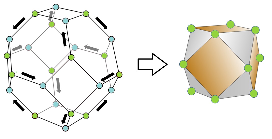
Figure 5: Coloring a truncated octahedron with 2 colors

Fig. 6 shows the relationship between the cuboctahedron and truncated octahedron. Starting from the octahedron, if we apply the uniform truncation, we obtain a truncated octahedron, which is also called a permutahedron (of order 4). If we continue to do deeper truncation, we can obtain the cuboctahedron as a result of rectified truncation. This truncation process also can be interpreted as moving metallic gold nodes on the silver nodes as in Fig. 5, which is a similar process of compressing the truncated octahedron from the eight cardinal directions to make a compact polytope (which is a cuboctahedron in this case) so that the metallic gold nodes are placed closest to each other.

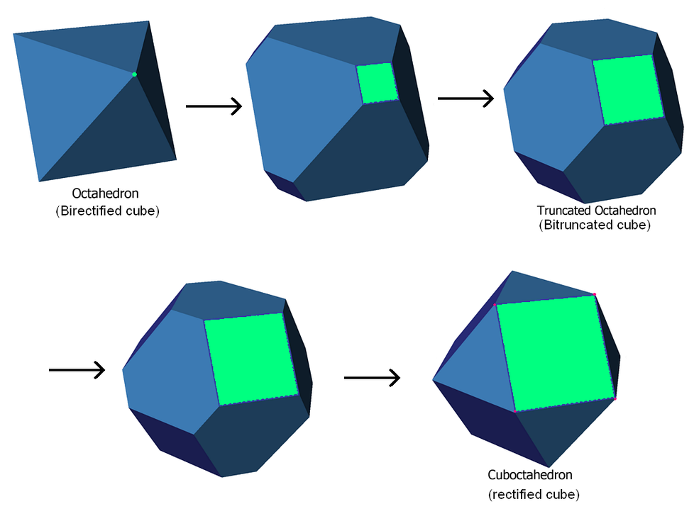
Figure 6: The truncation process of an octahedron

Then, based on the fact that the restricted chromatic number for the cuboctahedron is 3 (as in Fig. 7), we can re-color the metallic gold nodes with a different set of 3 colors (metallic gold, dark orchid, milano red) as on the right in Fig. 7. And if we process the same step on the silver vertices as Fig. 8, we can get a new set of 6 $(=2\times 3)$ colors for permutahedron coloring with the appropriate coloring position that satisfies the restricted coloring condition as Fig. 3 and maximizes the ${\cal G}{}_{(3)}$, which coincides with the second solution.

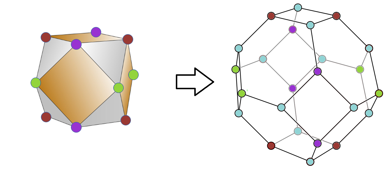
Figure 7: Re-coloring metallic gold nodes in Fig. 5 with 3 colors (metallic gold, dark orchid, milano red)

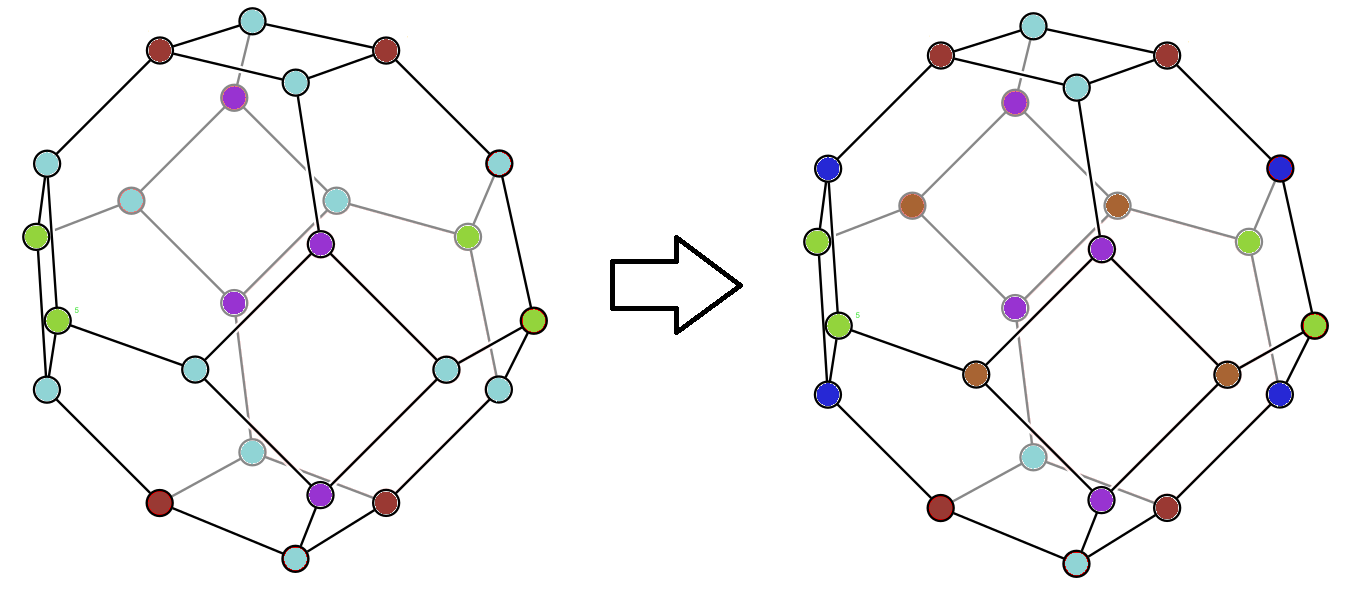
Figure 8: Re-coloring silver nodes in the Fig. 7 with 3 colors (silver, mai tai, persian blue)

This approach is one of the available polytopic approach to find the positions of six sets of matrices representing Clifford Algebras on the permutahedron, and it can also be applied to the higher dimensional permutahedra.

Interestingly there are many different research activities based on developing the properties of the chromatic number $\chi(G)$. For example, Brook’s Theorem states that the chromatic number of a graph is at most the maximum vertex degree, except when the graph is complete or an odd cycle. [?], and Grötzsch’s theorem states that a triangle-free planar graph can be colored with only three colors.  [?]

Thus, the importance of polytopic representation of the $N$-extended supermultiplets is the availability it provides for a bridge between various applications of mathematical fields of study such as graph theory, combinatorics, and supersymmetry. More detailed examples of SUSY representation will be presented in the remainder of the discussion.

2 Recursive Construction of Supermultiplets

Let us begin by discussing our use of the term “supermultiplet” in this work. Throughout the following, the term supermultiplet refers to a collection of matrices. The matrices in question are denoted by ${{\boldsymbol{{\rm L}}}}{}_{{}_{{\rm I}}}$ and ${{\boldsymbol{{\rm R}}}}{}_{{}_{{\rm I}}}$ where these are d $\times$ d matrices and the subscripted indices ${{{\rm I}}}$ take on values ${{{\rm I}}}$ = 1,…, $N$ (for some integer $N$). These matrices can be extended to a set of $N$ (2d) $\times$ (2d) matrices (denoted by ${\widehat{{\boldsymbol{\gamma}}}}{}_{\rm I}$) by use of the formula

 

$${{\widehat{{\boldsymbol{\gamma}}}}{}_{\rm I}~{}}$$

  (2.1)

for each collection ${{\boldsymbol{{\rm L}}}}{}_{{}_{{\rm I}}}$ and ${{\boldsymbol{{\rm R}}}}{}_{{}_{{\rm I}}}$. Here, the symbol $\otimes$ denotes the outer product where ${{\boldsymbol{\sigma}}}^{1}$ and ${{\boldsymbol{\sigma}}}^{2}$ are the usual first and second Pauli-matrices.

For our purposes, the collections ${{\boldsymbol{{\rm L}}}}{}_{{}_{{\rm I}}}$-${{\boldsymbol{{\rm R}}}}{}_{{}_{{\rm I}}}$ are distinguished into two types. When the collections satisfy (and thus form representations of Euclidean Clifford Algebras)

$$\left\{\,{\widehat{{\boldsymbol{\gamma}}}}{}_{\rm I}~{},~{}{\widehat{{\boldsymbol{\gamma}}}}{}_{\rm J}\,\right\}=2\,\delta_{\rm{IJ}}\,{{\boldsymbol{\rm{I}}}}{}_{2d}~{}~{}~{},$$ (2.2)

they are called an “off-shell” set. This condition is realized when the ${{\boldsymbol{{\rm L}}}}{}_{{}_{{\rm I}}}$-${{\boldsymbol{{\rm R}}}}{}_{{}_{{\rm I}}}$ matrices satisfy the equations

$$\begin{split}{{\boldsymbol{{\rm L}}}}{}_{{}_{{\rm I}}}\,{{\boldsymbol{{\rm R}}}}{}_{{}_{{\rm J}}}~{}+~{}{{\boldsymbol{{\rm L}}}}{}_{{}_{{\rm J}}}\,{{\boldsymbol{{\rm R}}}}{}_{{}_{{\rm I}}}&~{}=~{}2\,\delta{}_{{}_{\rm{I\,J}}}\,{{\boldsymbol{\rm{I}}}}{}_{\rm d}~{}~{}~{},~{}~{}~{}{{\boldsymbol{{\rm R}}}}{}_{{}_{{\rm I}}}\,{{\boldsymbol{{\rm L}}}}{}_{{}_{{\rm J}}}~{}+~{}{{\boldsymbol{{\rm R}}}}{}_{{}_{{\rm J}}}\,{{\boldsymbol{{\rm L}}}}{}_{{}_{{\rm I}}}~{}=~{}2\,\delta{}_{{}_{\rm{I\,J}}}\,{{\boldsymbol{\rm{I}}}}{}_{\rm d}~{}~{}~{}.\end{split}$$ (2.3)

In previous works, these have been called the ${\cal{GR}}$(d, $N$) or “garden algebra” conditions recognizing the dependence on the parameters $\rm{d}$ and $N$.

However, some of the sets in the following discussion satisfy a different condition of the form

$$\left\{\,{\widehat{{\boldsymbol{\gamma}}}}{}_{\rm I}~{},~{}{\widehat{{\boldsymbol{\gamma}}}}{}_{\rm J}\,\right\}=2\,\delta_{\rm{IJ}}\,{{\boldsymbol{\rm{I}}}}{}_{2\rm{d}}~{}+~{}{\cal N}{}_{\rm{IJ}}{}^{\widehat{\alpha}}\,{{\boldsymbol{\kappa}}}{}_{\widehat{\alpha}}~{}~{}~{},$$ (2.4)

where the coefficients ${\cal N}{}_{\rm{IJ}}{}^{\widehat{\alpha}\,({\cal R})}$ and the sets of $2\rm{d}$ $\times$ $2\rm{d}$ matrices ${{\boldsymbol{\kappa}}}{}_{\widehat{\alpha}}{}^{({\cal R})}$ are determined by the explicit forms of each ${{\boldsymbol{{\rm L}}}}{}_{{}_{{\rm I}}}$-${{\boldsymbol{{\rm R}}}}{}_{{}_{{\rm I}}}$ collection. In this case above, the collection is called an “on-shell” set. The coefficients ${\cal N}{}_{\rm{IJ}}{}^{\widehat{\alpha}\,({\cal R})}$ may be interpreted as obstructions of an off-shell set to forming a Clifford algebra.

It is worth noting that matrix collections of ${{\boldsymbol{{\rm L}}}}{}_{{}_{{\rm I}}}$ and ${{\boldsymbol{{\rm R}}}}{}_{{}_{{\rm I}}}$ that are $\rm d$ $\times$ $\rm d$ matrices can be regarded as special cases of more general matrices. In this more general case, the $\rm d$ $\times$ $\rm d$ ${{\boldsymbol{{\rm L}}}}{}_{{}_{{\rm I}}}$ matrices are replaced by ${\rm d}_{L}\times{\rm d}_{R}$ ${{\boldsymbol{{\rm L}}}}{}_{{}_{{\rm I}}}$ matrices where the integers ${\rm d}_{L}$ and ${\rm d}_{R}$ satisfy ${\rm d}_{L}$ $\neq$ ${\rm d}_{R}$ . In a similar manner in the more general case, the $\rm d$ $\times$ $\rm d$ ${{\boldsymbol{{\rm R}}}}{}_{{}_{{\rm I}}}$ matrices are replaced by ${\rm d}_{L}\times{\rm d}_{R}$ ${{\boldsymbol{{\rm R}}}}{}_{{}_{{\rm I}}}$ matrices. When this is done, the condition in (2.3) requires a replacement of the form

$$\begin{split}{{\boldsymbol{{\rm L}}}}{}_{{}_{{\rm I}}}\,{{\boldsymbol{{\rm R}}}}{}_{{}_{{\rm J}}}~{}+~{}{{\boldsymbol{{\rm L}}}}{}_{{}_{{\rm J}}}\,{{\boldsymbol{{\rm R}}}}{}_{{}_{{\rm I}}}&~{}=~{}2\,\delta{}_{{}_{\rm{I\,J}}}\,{{\boldsymbol{\rm{I}}}}{}_{{\rm d}_{L}}~{}~{}~{},~{}~{}~{}{{\boldsymbol{{\rm R}}}}{}_{{}_{{\rm I}}}\,{{\boldsymbol{{\rm L}}}}{}_{{}_{{\rm J}}}~{}+~{}{{\boldsymbol{{\rm R}}}}{}_{{}_{{\rm J}}}\,{{\boldsymbol{{\rm L}}}}{}_{{}_{{\rm I}}}~{}=~{}2\,\delta{}_{{}_{\rm{I\,J}}}\,{{\boldsymbol{\rm{I}}}}{}_{{\rm d}_{R}}~{}~{}~{}.\end{split}$$ (2.5)

but there have never been uncovered realization where it is possible to simultaneously satisfy both of these conditions. The situation ${\rm d}_{L}$ $\neq$ ${\rm d}_{R}$. occurs often when a collection of fields only realize the supersymmetry algebra subject to some set of dynamical equations. In the following, we will only consider the case were ${\rm d}_{L}$ = ${\rm d}_{R}$, but in distinction with most previous studies this does not insure the realization of an “off-shell” system.

It has been proposed that the structures above successfully “mirror” a situation that often occurs in discussions of supersymmetrical field theories when these are formulated in terms of the component fields of the representations. Adinkras are thus graphs defined over the component field space (but only gauge-invariant component fields) of SUSY representations. The parameter $\rm d$ counts the number of gauge-invariant field components independent of dynamics while $N$ counts the number of supercharges. The case of 4D, $\cal N$ = 1 supergravity can be used to illustrate this approach in an illuminating manner. Let us illustrate this “mirroring” in an explicit example provided by four dimensional “supergravity theory.”

The original presentations of the four dimensional supergravity theory were completed by Freedman, van Nieuwenhuizen, and Ferrara  [?] and Deser, and Zumino  [?] whose works were expressed in terms of the graviton $e{}_{\underline{a}}{}^{\underline{m}}(x)$ and the gravitino $\psi{}_{\underline{a}}{}^{\alpha}(x)$ fields. These works also contained the supersymmetry variations $\delta_{Q}e{}_{\underline{a}}{}^{\underline{m}}(x)$ and $\delta_{Q}\psi{}_{\underline{a}}{}^{\alpha}(x)$. Upon calculation of the commutator of two successive SUSY variations specified by fermionic Grassmann parameters $\epsilon_{1}$ and $\epsilon_{2}$ on either field variable one finds

$$\left[\,\delta_{Q}(\epsilon_{1})~{},~{}\delta_{Q}(\epsilon_{2})\,\right]~{}=~{}i\,2\left(\epsilon_{1}\,\gamma^{\underline{a}}\,\epsilon_{2}\,\right)\,e{}_{\underline{a}}{}^{\underline{m}}\partial{}_{\underline{m}}~{}+~{}\delta{}_{\rm{Gauge}}~{}+~{}{\delta\,{\cal L}}{}_{{\rm field}}$$ (2.6)

where ${\delta{}_{\rm{Gauge}}}$ denotes an appropriate gauge transformation for each field, and ${\delta\,{\cal L}}{}_{{\rm field}}$ denotes the variation of a Lagrangian with respect to the fermionic field, but not the bosonic field, on which the commutators are being evaluated.

Since adinkras are defined only over the gauge-invariant component fields, the first term on the RHS in (2.6) has been proposed as the hologram of the first term on the RHS of (2.4). Since adinkras only contain the gauge-invariant components, the second term on the RHS of (2.6) vanishes identically. Finally, the final term on the RHS of (2.6) has been proposed as the hologram of the last term on the RHS of (2.4).

Starting with the discussions [?] and  [?], it has been found that in a number of cases the ${{\boldsymbol{{\rm R}}}}{}_{{}_{{\rm I}}}$ matrices are the matrix transpose of the ${{\boldsymbol{{\rm L}}}}{}_{{}_{{\rm I}}}$ matrices and furthermore the latter can be considered signed permutations, i.e. elements of Coxeter groups. In the case where ${{\rm I}}$ and $\rm d$ take on values 1,…,4, the elements of the corresponding Coxeter Group can be “broken” into six distinct sets

$$\{CM\}=\{\langle 1\bar{4}2\bar{3}\rangle,\langle 23\bar{1}\bar{4}\rangle,\langle 3\bar{2}\bar{4}1\rangle,\langle 4132\rangle\}$$ (2.7)

$$\{TM\}=\{\langle 1\bar{3}\bar{4}\bar{2}\rangle,\langle 24\bar{3}1\rangle,\langle 312\bar{4}\rangle,\langle 4\bar{2}13\rangle\}$$ (2.8)

$$\{VM\}=\{\langle 13\bar{2}\bar{4}\rangle,\langle 2\bar{4}1\bar{3}\rangle,\langle 3\bar{1}\bar{4}2\rangle,\langle 4231\rangle\}$$ (2.9)

$$\left\{VM_{1}\right\}=\{\langle 1\bar{4}\bar{3}2\rangle,\langle\bar{2}\bar{3}41\rangle,\langle 3\bar{2}1\bar{4}\rangle,\langle 4123\rangle\}$$ (2.10)

$$\left\{VM_{2}\right\}=\{\langle 12\bar{4}\bar{3}\rangle,\langle\bar{2}13\bar{4}\rangle,\langle 3421\rangle,\langle 4\bar{3}1\bar{2}\rangle\}$$ (2.11)

$$\left\{VM_{3}\right\}=\{\langle 12\bar{3}\bar{4}\rangle,\langle\bar{2}1\bar{4}3\rangle,\langle 3412\rangle,\langle 4\bar{3}\bar{2}1\rangle\}$$ (2.12)

(the notation and definitions of these can be found in the work of  [?]) whose union is the complete Coxeter group. Taking the absolute values of the Coxeter group elements in this discussion leads to the permutation group of order four. The foundational tool used in  [?] to discover the dissection of this Coxeter group, and its permutation subgroup, caused by the condition in (2.3) was a computer code used to find all of its solutions.

In the end, this dissection process is equivalent to a sorting problem. The $4!$ elements of the permutation group of order four are sorted into six (i.e. 3!) disjointed subsets each containing four elements. The equivalent problem related to the work completed in  [?] must begin with the $8!=40,320$ elements of the permutation group of order eight sorted into 5,040 (i.e. 7!) disjointed subsets each containing eight elements.

We begin noting some of the results for $\cal N$ = 2 supermultiplets for supersymmetry  [?], which for the chiral-chiral (CC), chiral-vector (CV) and chiral-tensor (CT) supermultiplets are given by

$$\begin{aligned} &\mathbf{L}^{CC}_{1}=(170)_{b}\langle 14235867\rangle\\ &\mathbf{L}^{CC}_{2}=(204)_{b}\langle 23146758\rangle\\ &\mathbf{L}^{CC}_{3}=(102)_{b}\langle 32417685\rangle\\ &\mathbf{L}^{CC}_{4}=(0)_{b}\langle 41328576\rangle\\ &\mathbf{L}^{CC}_{5}=(15)_{b}\langle 58671423\rangle\\ &\mathbf{L}^{CC}_{6}=(105)_{b}\langle 67582314\rangle\\ &\mathbf{L}^{CC}_{7}=(195)_{b}\langle 76853241\rangle\\ &\mathbf{L}^{CC}_{8}=(165)_{b}\langle 85764132\rangle\end{aligned}\qquad\qquad\begin{aligned} &\mathbf{L}^{CV}_{1}=(170)_{b}\langle 14236857\rangle\\ &\mathbf{L}^{CV}_{2}=(204)_{b}\langle 23145768\rangle\\ &\mathbf{L}^{CV}_{3}=(6)_{b}\langle 32418675\rangle\\ &\mathbf{L}^{CV}_{4}=(96)_{b}\langle 41327586\rangle\\ &\mathbf{L}^{CV}_{5}=(210)_{b}\langle 58672413\rangle\\ &\mathbf{L}^{CV}_{6}=(180)_{b}\langle 67581324\rangle\\ &\mathbf{L}^{CV}_{7}=(126)_{b}\langle 76854231\rangle\\ &\mathbf{L}^{CV}_{8}=(24)_{b}\langle 85763142\rangle\end{aligned}\qquad\qquad\begin{aligned} &\mathbf{L}^{CT}_{1}=(234)_{b}\langle 14235786\rangle\\ &\mathbf{L}^{CT}_{2}=(76)_{b}\langle 23146875\rangle\\ &\mathbf{L}^{CT}_{3}=(134)_{b}\langle 32417568\rangle\\ &\mathbf{L}^{CT}_{4}=(32)_{b}\langle 41328657\rangle\\ &\mathbf{L}^{CT}_{5}=(11)_{b}\langle 58671342\rangle\\ &\mathbf{L}^{CT}_{6}=(173)_{b}\langle 67582431\rangle\\ &\mathbf{L}^{CT}_{7}=(103)_{b}\langle 76853124\rangle\\ &\mathbf{L}^{CT}_{8}=(193)_{b}\langle 85764213\rangle\end{aligned}$$ (2.13)

The elements of the garden algebra, being a subgroup of the Coxeter group, are composed of a signed matrix (the boolean factors in the above equations) times a permutation matrix, which together form the Coxeter group elements. Our method of generating higher $N$ supermultiplets will split the process into two parts. We generate the permutation matrices and the boolean factors separately, then combine the two. First we will examine the process of generating the analogous elements of higher $N$ permutation matrices.

Finally, it is of note that the ${{\boldsymbol{{\rm L}}}}{}_{{}_{{\rm I}}}$-${{\boldsymbol{{\rm R}}}}{}_{{}_{{\rm I}}}$ matrices associated with the (CC) set satisfy the equations in (2.13) while those associated with both the (CV) and (CT) sets satisfy the equations in (2.2).

This is in accord with the observation well known in the physics literature that there is no known off-shell formulation of the so-called 4D, ${\cal N}$ = 2 “hypermultiplet” described solely in terms of eight component fields. On the other hand, it is well known that there exist off-shell formulations of the so-called 4D, ${\cal N}$ = 2 vector supermultiplet and the 4D, ${\cal N}$ = 2 tensor supermultiplet in terms of eight component fields.

2.1 Generating higher SUSY permutation matrices from lower ones

We begin by demonstrating the process for recursively constructing the chiral-chiral $\cal N$=2 supermultiplets from the chiral $\cal N$=1 supermultiplet. Concatenating two copies of the first element of (2.7) (and ignoring the boolean factor represented by the overlined numbers for now), we have

$$\begin{aligned} \langle 1423\rangle\oplus\langle 1423\rangle=\langle 14231423\rangle\end{aligned}\qquad\rightarrow\qquad\begin{aligned} \langle 1423\rangle\oplus\langle 5867\rangle=\langle 14235867\rangle\end{aligned}$$ (2.14)

where we relabeled our second string so that our numbering would be from 1-8. We see that this indeed matches the permutation matrix component of $\mathbf{L}^{CC}_{1}$ above. For matrices $\mathbf{L}^{CC}_{5}-\mathbf{L}^{CC}_{8}$ we instead relabel the first string (adding 4 to the first four numbers instead of the last four). Similar manipulations can be carried out for all the remaining supermultiplets, notably even when we are combining different $\cal N$=1 supermultiplets. For example, to generate $|\mathbf{L}_{1}^{CT}|$, we combine

$$\begin{aligned} \langle 1423\rangle\oplus\langle 1342\rangle=\langle 14231342\rangle\end{aligned}\qquad\rightarrow\qquad\begin{aligned} \langle 1423\rangle\oplus\langle 5786\rangle=\langle 14235786\rangle\end{aligned}$$ (2.15)

which matches with what was previously found for $\mathbf{L}_{1}^{CT}$ up to the boolean factor.

This process is also applied to the creation of the $\mathbf{L}_{2}^{CT}$, $\mathbf{L}_{3}^{CT}$, and $\mathbf{L}_{4}^{CT}$ matrices. By this means we have gone from four 4 $\times$ 4 matrices to four 8 $\times$ 8 matrices.

The corresponding $|\mathbf{L}_{5}^{CT}|$ is found from relabeling the first string instead

$$\begin{aligned} \langle 1423\rangle\oplus\langle 1342\rangle=\langle 14231342\rangle\end{aligned}\qquad\rightarrow\qquad\begin{aligned} \langle 5867\rangle\oplus\langle 1342\rangle=\langle 58671342\rangle\end{aligned}$$ (2.16)

which indeed matches the permutation element of the 4D, $\cal N$ = 2 chiral-tensor supermultiplet given above. We apply this process to the creation of the $\mathbf{L}_{6}^{CT}$, $\mathbf{L}_{7}^{CT}$, and $\mathbf{L}_{8}^{CT}$ matrices. Now we have four more 8 $\times$ 8 matrices.

The discussion above was carried out on the basis of considering the matrices as realizations of permutation operators. We can summarize these results in the forms of formulae applied to matrices, but without any reference to permutations. The discussion above directly implies

$$|{\widehat{{\boldsymbol{L}}}}^{(multp1,multp2)}_{\rm I}|~{}=~{}\frac{1}{2}\,(\,{{\boldsymbol{\rm I}}}\,+\,{{\boldsymbol{\sigma}}}^{3}\,)\,\otimes\,|{{\boldsymbol{{\rm L}}}}_{\rm I}^{(multp1)}|~{}+~{}\frac{1}{2}\,(\,{{\boldsymbol{\rm I}}}\,-\,{{\boldsymbol{\sigma}}}^{3}\,)\,\otimes\,|{{\boldsymbol{{\rm L}}}}_{\rm I}^{(multp2)}|~{}~{}~{}~{}~{}~{}~{}~{}~{},~{}~{}~{}{\rm{for}}~{}{\rm I}~{}=~{}1,...,4~{}~{}~{},$$ (2.17)

$$|{\widehat{{\boldsymbol{L}}}}^{(multp1,multp2)}_{\rm I}|~{}=~{}\hbox{\large{${\frac{{1}}{{\sqrt{2}}}}$}}\,(\,{{\boldsymbol{\sigma}}}^{-}\,)\,\otimes\,|{{\boldsymbol{{\rm L}}}}_{\rm I}^{(multp1)}|~{}+~{}\hbox{\large{${\frac{{1}}{{\sqrt{2}}}}$}}\,(\,{{\boldsymbol{\sigma}}}^{+}\,)\,\otimes\,|{{\boldsymbol{{\rm L}}}}_{\rm I}^{(multp2)}|~{}~{}~{}~{}~{}~{}~{}~{}~{}~{}~{}~{}~{}~{}~{}~{},~{}~{}~{}{\rm{for}}~{}{\rm I}~{}=~{}5,...,8~{}~{}~{}.$$

Here “multp1”, “multp2” denote the lower SUSY permutation matrices we use. At this point, it is also convenient to introduce a notational device that will be convenient later. Upon making the definitions

$${{\boldsymbol{\rm P}}}{}^{\pm}~{}\equiv~{}\frac{1}{2}\,(\,{{\boldsymbol{\rm I}}}\,\pm\,{{\boldsymbol{\sigma}}}^{3}\,)$$ (2.18)

we can rewrite (2.17) in the form

$$|{\widehat{{\boldsymbol{L}}}}^{(multp1,multp2)}_{\rm I}|~{}=~{}{{\boldsymbol{\rm P}}}{}^{+}\,\otimes\,|{{\boldsymbol{{\rm L}}}}_{\rm I}^{(multp1)}|~{}+~{}{{\boldsymbol{\rm P}}}{}^{-}\otimes\,|{{\boldsymbol{{\rm L}}}}_{\rm I}^{(multp2)}|~{}~{}~{}~{}~{}~{}~{}~{}~{}~{}~{}~{}~{}~{}~{}~{}~{}~{}~{}~{}~{}~{}~{}~{}~{},~{}~{}~{}{\rm{for}}~{}{\rm I}~{}=~{}1,...,4~{}~{}~{},$$ (2.19)

$$|{\widehat{{\boldsymbol{L}}}}^{(multp1,multp2)}_{\rm I}|~{}=~{}\hbox{\large{${\frac{{1}}{{\sqrt{2}}}}$}}\,(\,{{\boldsymbol{\sigma}}}^{-}\,)\,\otimes\,|{{\boldsymbol{{\rm L}}}}_{\rm I}^{(multp1)}|~{}+~{}\hbox{\large{${\frac{{1}}{{\sqrt{2}}}}$}}\,(\,{{\boldsymbol{\sigma}}}^{+}\,)\otimes\,|{{\boldsymbol{{\rm L}}}}_{\rm I}^{(multp2)}|.~{}~{}~{}~{}~{}~{}~{}~{}~{},~{}~{}~{}{\rm{for}}~{}{\rm I}~{}=~{}5,...,8~{}~{}~{}.$$

where we have used the ${{\boldsymbol{\rm P}}}$ notation to distinguish these matrices from elements in the permutation group such as appearing in (2.20) below. The reader is reminded that these results  [?] follow from two steps starting with the linear addition of pairs of actions for 4D, $\cal N$ = 1 off-shell supermultiplets. First one obtains fermionic transformation laws that leave the pairs of actions invariant up to surface terms and then one reduces these transformation laws to one dimension to obtain the corresponding L-matrices. Starting from the 4D, $\cal N$ = 1 off-shell chiral, vector, and tensor supermultiplets, this leads to six sets of L-matrices. We denote these matrices according to the pairings of the supermultiplets, hence (CC), (CV), (CT), (VV), (VT), (TT). We may think of these as labeling different representations. The work in  [?] (that is based solely on considerations from purely one-dimensional SUSY) was the source of a seventh set of matrices, and we can call this the (O) (for original) representation. The absolute values of all seven sets lie within the permutation group of order eight. However, only the (O), (CV), (CT) sets satisfy the garden algebra condition that marks them as being ‘off-shell’ representations.

2.2 Generating the boolean factor for higher dimensional supermultiplets

While in Sec. 2.1 we have recursively generated the unsigned L-matrices, the boolean factors are slightly more complicated to generate. We illustrate the general recursive construction for the Chiral-Tensor $\cal N$=2 supermultiplet. We first note that signed L-matrices can be decomposed into a sign factor matrix (boolean factor) times a permutation group matrix [?], i.e,

$$\left(\mathbf{L}_{\mathrm{I}}\right)_{i}{}^{\hat{k}}=\left(\mathcal{S}^{(\mathrm{I})}\right)_{i}{}^{{\ell}}\left(\mathcal{P}_{(\mathrm{I})}\right)_{{\ell}}{}^{\hat{k}}$$ (2.20)

We generate the boolean factors from the sign factor matrices as follows:

$$\left(\mathcal{S}^{(\mathrm{I})}\right)_{i}{}^{{\ell}}=\left[\begin{array}[]{cccc}(-1)^{b_{1}}&0&0&\cdots\\ 0&(-1)^{b_{2}}&0&\cdots\\ 0&0&(-1)^{b_{2}}&\cdots\\ \vdots&\vdots&\vdots&\ddots\end{array}\right]\quad\leftrightarrow\quad\left(\mathcal{R}_{\mathrm{I}}=\sum_{i=1}^{\mathrm{d}}b_{i}2^{i-1}\right)_{b}=\begin{array}[]{c}{\left[b_{1}b_{2}\cdots b_{\mathrm{d}}\right]_{2}},\end{array}$$ (2.21)

Here in (2.21) $\mathcal{R}_{\mathrm{I}}$ represent the arbitrary real number, where we read binary words from left to right by convention (in contrast to the typical right to left construction). For example we can consider the decomposition of $\mathbf{L}_{1}$ for the $\cal N$=1 chiral multiplet, for which we have

$$\left(\mathbf{L}_{1}\right)_{i}{}^{\hat{k}}=\left[\begin{array}[]{cccc}1&0&0&0\\ 0&0&0&-1\\ 0&1&0&0\\ 0&0&-1&0\end{array}\right]=\left[\begin{array}[]{cccc}1&0&0&0\\ 0&-1&0&0\\ 0&0&1&0\\ 0&0&0&-1\end{array}\right]\left[\begin{array}[]{cccc}1&0&0&0\\ 0&0&0&1\\ 0&1&0&0\\ 0&0&1&0\end{array}\right]=(10)_{b}\langle 1423\rangle=\langle 1\overline{4}2\overline{3}\rangle.$$ (2.22)

Turning now to the construction of $\mathbf{L}_{1}$ for the $\cal N$=2 chiral-tensor,

$$\begin{split}\mathbf{L}_{1}^{(CT)}&=\langle 1\bar{4}2\bar{3}\rangle\oplus\langle 1\bar{3}\bar{4}\bar{2}\rangle\\ &=[01010111]_{b}\langle 14235786\rangle\end{split}$$ (2.23)

where $[01010111]_{b}$ means the boolean factor [01010111]. Going forward we will bracket these factors and give them a subscript of b.

In the following, ${{\boldsymbol{\cal B}}}_{{{\boldsymbol{\cal(R)}}}}$ corresponds to a bitflip matrix (for given representation $\cal R$) obtained in the following way. To take the Chiral-Vector multiplet as an example, for elements $\mathbf{L}^{(CT)}_{5}-\mathbf{L}^{(CT)}_{8}$ we use the following rule: For the $i$-th element, take the $(i-4)$-th element’s boolean factor and flip 4 neighboring bits (for example the fifth through the eighth bits. The choice of where to start is arbitrary). Do this to generate the boolean factors for $\mathbf{L}^{(CT)}_{5}-\mathbf{L}^{(CT)}_{8}$ and check if the garden algebra closes. If it does not close, cycle the choice of neighboring bits by one. For our example of choosing the fifth through the eighth bits, we would get a factor that wouldn’t satisfy the garden algebra. Therefore we’d cycle to the next 4 neighboring bits, {6, 7, 8, 1}. In principle, there are 8 choices to cycle through (i.e {1, 2, 3, 4},{2, 3, 4, 5},{3, 4, 5, 6},{4, 5, 6, 7},{5, 6, 7, 8},{6, 7, 8, 1},{7, 8, 1, 2},{8, 1, 2, 3}) for $\cal N$=2. If none of these combinations work, then the supermultiplet does not have boolean factors that make it a garden algebra. The example calculation for $\mathbf{L}^{(CT)}_{5}$ ($\cal N$=2 chiral-tensor) is performed below, where we apriori know that the correct bits to flip are (6, 7, 8, 1).

$$\begin{split}\mathbf{L}_{5}^{(CT)}&=\langle 1\bar{4}2\bar{3}\rangle\oplus\langle 1\bar{3}\bar{4}\bar{2}\rangle\\ &=\text{Bitflip}_{(6,7,8,1)}([01010111]_{b})\langle 58671342\rangle\\ &=[11010000]_{b}\langle 58671342\rangle\end{split}$$ (2.24)

The corresponding bitflip matrices for the (CV) and (CT) sets take the respective forms

$${{\boldsymbol{\cal B}}}_{(CV)}=\begin{bmatrix}1&0&0&0&0&0&0&0\\ 0&1&0&0&0&0&0&0\\ 0&0&1&0&0&0&0&0\\ 0&0&0&-1&0&0&0&0\\ 0&0&0&0&-1&0&0&0\\ 0&0&0&0&0&-1&0&0\\ 0&0&0&0&0&0&-1&0\\ 0&0&0&0&0&0&0&1\end{bmatrix}~{}~{}~{},~{}~{}~{}{{\boldsymbol{\cal B}}}_{(CT)}=\begin{bmatrix}-1&0&0&0&0&0&0&0\\ 0&1&0&0&0&0&0&0\\ 0&0&1&0&0&0&0&0\\ 0&0&0&1&0&0&0&0\\ 0&0&0&0&1&0&0&0\\ 0&0&0&0&0&-1&0&0\\ 0&0&0&0&0&0&-1&0\\ 0&0&0&0&0&0&0&-1\end{bmatrix}.$$ (2.25)

The boolean factors of $\mathbf{L}^{(CT)}_{5}-\mathbf{L}^{(CT)}_{8}$ are dual to the boolean factors of $\mathbf{L}^{(CT)}_{1}-\mathbf{L}^{(CT)}_{4}$ by doubly even (4) bit flips on neighboring bits.

It is obvious that these matrices square to the identity element and as well are traceless. Let us rewrite these in the outer product notation in the forms

$${{\boldsymbol{\cal B}}}_{(CV)}~{}=~{}(\,{{\boldsymbol{\rm P}}}{}^{+}\,)\,\otimes\,{{\boldsymbol{{\cal M}}}}_{{{\boldsymbol{\cal(CV)}}}}~{}+~{}(\,{{\boldsymbol{\rm P}}}{}^{-}\,)\,\otimes\,{{\boldsymbol{\widetilde{\cal M}}}}_{{{\boldsymbol{\cal(CV)}}}}$$ (2.26)

$${{\boldsymbol{\cal B}}}_{(CT)}~{}=~{}(\,{{\boldsymbol{\rm P}}}{}^{+}\,)\,\otimes\,{{\boldsymbol{\cal M}}}_{{{\boldsymbol{\cal(CT)}}}}~{}+~{}(\,{{\boldsymbol{\rm P}}}{}^{-}\,)\,\otimes\,{{\boldsymbol{\widetilde{\cal M}}}}_{{{\boldsymbol{\cal(CT)}}}}$$ (2.27)

The quantities ${{\boldsymbol{\widetilde{\cal M}}}}_{{{\boldsymbol{\cal(CV)}}}}$ and ${{\boldsymbol{\widetilde{\cal M}}}}_{{{\boldsymbol{\cal(CT)}}}}$ are the bitflip duals of ${{\boldsymbol{{\cal M}}}}_{{{\boldsymbol{\cal(CV)}}}}$ and ${{\boldsymbol{{\cal M}}}}_{{{\boldsymbol{\cal(CT)}}}}$ and in these equations ${{\boldsymbol{{\cal M}}}}_{{{\boldsymbol{\cal(CV)}}}}$ and ${{\boldsymbol{{\cal M}}}}_{{{\boldsymbol{\cal(CT)}}}}$ are the 4 $\times$ 4 matrices given by

$${{\boldsymbol{\cal M}}}_{{{\boldsymbol{\cal(CV)}}}}~{}=~{}\begin{bmatrix}1&0&0&0\\ 0&1&0&0\\ 0&0&1&0\\ 0&0&0&-1\end{bmatrix}~{}~{}~{},~{}~{}~{}{{\boldsymbol{\cal M}}}_{{{\boldsymbol{\cal(CT)}}}}~{}=~{}\begin{bmatrix}-1&0&0&0\\ 0&1&0&0\\ 0&0&1&0\\ 0&0&0&1\end{bmatrix}$$ (2.28)

These matrices make it clear that the form of the ${{\boldsymbol{\cal M}}}_{({{\boldsymbol{{\cal R}}}})}$ matrices determine the forms of the ${{\boldsymbol{\widetilde{\cal M}}}}_{({{\boldsymbol{\cal R}}})}$ matrices (and thus the forms of the ${{\boldsymbol{\cal B}}}_{({\cal R})}$ matrices) for the representations $({\cal R})$ = $({CV})$ and $({CT})$.

In terms of matrix notation, we have

$${\widehat{{\boldsymbol{\cal S}}}}{}_{\rm I}~{}=~{}(\,{{\boldsymbol{\rm P}}}{}^{+}\,)\,\otimes\,{{\boldsymbol{\cal S}}}_{\rm I}^{(multp1)}~{}+~{}(\,{{\boldsymbol{\rm P}}}{}^{-}\,)\,\otimes\,{{\boldsymbol{\cal S}}}_{\rm I}^{(multp2)}~{}~{}~{}~{}~{}~{}~{}~{}~{},~{}~{}~{}{\rm{for}}~{}{\rm I}~{}=~{}1,...,4$$ (2.29)

$${\widehat{{\boldsymbol{\cal S}}}}{}_{\rm I}~{}=~{}(\,{{\boldsymbol{\rm P}}}{}^{+}\,)\,\otimes\,{{\boldsymbol{\cal M}}}_{{{\boldsymbol{\cal(R)}}}}\cdot{{\boldsymbol{\cal S}}}_{\rm I}^{(multp1)}~{}+~{}(\,{{\boldsymbol{\rm P}}}{}^{-}\,)\,\otimes\,{{\boldsymbol{\cal M}}}_{{{\boldsymbol{\cal(R)}}}}\cdot{{\boldsymbol{\cal S}}}_{\rm I}^{(multp2)}~{}~{}~{}~{}~{}~{}~{}~{}~{},~{}~{}~{}\\ {\rm{for}}~{}{\rm I}~{}=~{}5,...,8$$ (2.30)

According to equations (3.3) and (3.6) in  [?], we obtain the HYMN value for each supermultiplet representation. This allows the following dissection:

$${{\boldsymbol{\cal\hat{C}}}}^{{\boldsymbol{(}}CT)}={{\boldsymbol{\cal\hat{C}}}}^{(CV)}={{\boldsymbol{\cal\hat{C}}}}^{(O)}=\sigma_{3}\otimes{\bf{I}}_{8},$$ (2.31)

$${{\boldsymbol{\cal\hat{C}}}}^{(CC)}={{\boldsymbol{\cal\hat{C}}}}^{(TT)}={{\boldsymbol{\cal\hat{C}}}}^{(TV)}={{\boldsymbol{\cal\hat{C}}}}^{(VV)}={\bf{I}}_{16}$$ (2.32)

Here, the matrix denoted by ${\boldsymbol{\cal\hat{C}}}^{(\cal R)}$ is associated with each supermultiplet $\cal R$ and has eigenvalues known as HYMN values. [?]

The first class includes (CT), (CV), and (O), for which the HYMN matrix takes the form $\sigma_{3}\otimes{\bf{I}}_{8}$. The second class includes (CC), (TT), (TV), and (VV), for which the HYMN matrix takes the form ${\bf{I}}_{16}$. Based on the results presented in (2.2), the available bitflip for (CT) was {6, 7, 8, 1}. Although this is not a mathematical proof, it is an observation that works for (CT), (CV), and (O), but not for any other combinations.

As part of our investigation, it is necessary to classify other supermultiplets such as CMN, O($2n$), and Harmonic $N$=2 systems using the Hexipentisteriruncicantitruncated 7-Simplex. We anticipate that this classification will align with the HYMN value classification and demonstrate a clear correlation between the two methods.

2.3 A curious property maintained by the recursive construction

There is a curious mathematical property maintained by the six supermultiplets mentioned from (2.7) to (2.12). If we focus on the permutation matrices within a single representation, we can always pair the $n$-th matrix to $n$-th to last matrix so that the sum of the order of their “weight” (see Sec. 3.1) is $d!+1$, where $d$ is the dimension of the permutation. Take $\left\{VM_{1}\right\}=\{\langle 1234\rangle,\langle 2143\rangle,\langle 3412\rangle,\langle 4321\rangle\}$ for example. $\langle 1234\rangle$ is the smallest possible bracket notation for permutation of order $4$ and $\langle 4321\rangle$ is the largest. So after we arrange all permutations from smallest to largest, the orders of $\langle 1234\rangle$ and $\langle 4321\rangle$ are $1$ and $4!$ respectively. Their sum is $4!+1$. On the other hand, the orders of $\langle 2143\rangle$, $\langle 3412\rangle$ are $7$ and $18$ respectively. Still their sum is $4!+1$.

Another way of stating this property is that we can always pair the bracket notation so that the sum of digits on any position is $d+1$. For example, one pair within the VV supermultiplet  [?] is $|\mathbf{L}_{3}^{(VV)}|=\langle 42318675\rangle$ and $|\mathbf{L}_{6}^{(VV)}|=\langle 57681324\rangle$ (ignoring the boolean factor). The first digit of 42318675 is 4 and the first digit of 57681324 is 5. The sum of their first digits is the dimension plus 1: $4+5=8+1$, as well as the sum of 6-th digit $6+3=8+1$.

These two statements are equivalent. If we send every digit $i$ in braket notation to $d+1-i$, for instance $45728613$ maps to $54271386$, by symmetry the order of the preimage counting from small to large is exactly the order of the image counting from large to small.

This rule is preserved by our construction as well. Suppose we combine two $\cal N$=1 to obtain a $\cal N$=2 supermultiplet, and the two “ingredients” $\cal N$=1 satisfy the rule mentioned above. We can pair the $n$-th (for some $n\leq 4$) L-matrix of the newly obtained supermultiplet with the $(8-i+1)$-th L-matrix (note that $d$=8 here). Since the ‘ingredients’ satisfy the rule, by our construction method we know that the sum of the original digits at the same position would be $4+1$. On the other hand, the last half digits of the $n$-th L-matrix would be added $4$ from the original $\cal N$=1 matrix, whereas the first half digits of the $(8-i+1)$-th are added $4$. So the sum of digits at the same position of this pair would be $(4+1)+4=8+1$, maintaining the rule.

3 Hopping Operators and a General Construction

3.1 Introducing hopping operators

Within the domain of compact Lie algebras, the concepts of root and weight spaces, the maximal torus, etc. have been recognized for decades as valuable tools to construct the representation theories of these algebras. The Jordan-Chevelley Decomposition of the generators of these Lie algebras into elements of the maximal torus accompanied by an associated set of “raising” and “lowering” operators continually show their value as the foundations of Cartan’s classification of all compact Lie algebras.

Starting in a lecture entitled “Genomics, Networks, And Computational Concepts For Polytopic SUSY Representation Theory,” delivered in 2021  [?] it was proposed that although SUSY algebras are distinctly different from compact Lie algebras, the concept of a “weight space” does likely exist, even though (to the authors’ best knowledge) the analog of the Jordan-Chevelley decomposition apparently does not exist for SUSY algebras. Nevertheless, due to the relation of adinkras to Coxeter groups  [?], a structure has been identified for supersymmetry to play the role of root and weight spaces. An argument for such a structure goes as follows.

The elements of Coxeter groups may be regarded as signed permutations. Thus the Coxeter group of length-$d$ elements—which we denote here by BC($d$)—consists of $2^{d}\,d!$ elements. Taking the absolute values of the elements of BC($d$) yields the of the permutation group, which we denoted by $S_{d}$. There is a well-known polytope called the “permutahedron”  [?] associated with $S_{d}$. It was proposed in the works of  [?,?] that the permutahedron can act as a weight space/root space for adinkras. In order to achieve further progress along these lines, it becomes a pressing matter to define quantities that can play the role of “raising and lowering operators”. What defines the lowest or highest weight state of a representation? In particular, is there an intrinsic way to define the weight of a permutation operator?

There are two natural ways to denote permutation operators: (a) cycle notation, and (b) “bra-ket” notation. As an example, let us consider the set of permutations given in cycle notation by

 

$${\left\{{~{}~{}}\mathcal{P}_{1}=()~{},~{}~{}\mathcal{P}_{2}=(12)(34)~{},~{}~{}\mathcal{P}_{3}=(13)(24)~{},~{}~{}\mathcal{P}_{4}=(14)(23){~{}~{}}\right\}~{}~{}~{},}$$

  (3.1)

which in “bra-ket” notation can be rewritten as

 

$${\left\{{~{}}\langle 1234\rangle,~{}\langle 2143\rangle,~{}\langle 3412\rangle,~{}\langle 4321\rangle{~{}}\right\}~{}~{}~{},}$$

  (3.2)

respectively. It should be apparent that the “bra-ket” notation provides a natural mapping between permutation operators and natural numbers, obtained by treating the list of digits in the brackets as a number in base-$d$. We will refer to this map as the BK-map. The BK-map thus induces a ‘weight’ for each permutation, given by the order of their corresponding natural numbers. Elements can be ordered according to their weight defined by the BK-map. Inexorably, one is led to the concept that there is always a element of lightest weight that is natural and intrinsic in the considerations of permutations.

For example, application of the BK-map to the set in (3.1) leads to the set of numbers given by

 

$${\left\{{~{}}1234,~{}2143,~{}3412,~{}4321{~{}}\right\}~{}~{}~{}.}$$

  (3.3)

So it is seen that the set of permutations given by (3.1) is already correctly ordered according by this weight.

This fact leads one to realize given any construction involving permutations, the elements can be ordered according to their weight defined by the BK-map. Inexorably, one is led to the concept that there is always a element of lightest weight that is natural and intrinsic in the considerations of permutations.

Now we are in position to define “hopping operators” or “hoppers.” There are two sets of such operators: left hopping operators and right hopping operators. We denote the A-th left “hoppers” by the symbol ${\mathcal{H}}{}^{(L)}_{\rm A}$ and the A-th right “hoppers” by the symbol ${\mathcal{H}}{}^{(R)}_{\rm A}$. The hoppers are defined by the equations (where $\mathcal{P}_{1}$ is the permutation operator of lightest weight in a given set),

$${\mathcal{P}_{\rm A}~{}=~{}{\mathcal{H}}{}^{(L)}_{\rm A}\,\mathcal{P}_{1}~{}~{}~{}~{},~{}~{}~{}\mathcal{P}_{\rm A}~{}=~{}\mathcal{P}_{1}\,{\mathcal{H}}{}^{(R)}_{\rm A}~{}~{}~{},}$$ (3.4)

so the hopping operators can be calculated from the permutation elements via the equations

$${\mathcal{P}_{\rm A}\,\left[\mathcal{P}_{1}\right]{}^{-1}~{}=~{}{\mathcal{H}}{}^{(L)}_{\rm A}\,~{}~{}~{},~{}~{}~{}\left[\mathcal{P}_{1}\right]{}^{-1}\,\mathcal{P}_{\rm A}~{}=~{}{\mathcal{H}}{}^{(R)}_{\rm A}~{}~{}~{}.}$$ (3.5)

Before we leave this introduction to hoppers, it is of note that these operators have appeared in previous works on adinkras  [?,?,?,?,?,?]. In these older works the concepts of “bosonic holoraumy matrices” (${\mathbf{\cal B}}{\,}_{{}_{\rm{I\,J}}}$) and “fermionic holoraumy matrices” (${\mathbf{\cal F}}{\,}_{{}_{\rm{I\,J}}}$) were introduced and defined by

$$\begin{split}{{\boldsymbol{{\rm L}}}}{}_{{}_{{\rm I}}}\,{{\boldsymbol{{\rm R}}}}{}_{{}_{{\rm J}}}~{}-~{}{{\boldsymbol{{\rm L}}}}{}_{{}_{{\rm J}}}\,{{\boldsymbol{{\rm R}}}}{}_{{}_{{\rm I}}}&~{}=~{}{\mathbf{\cal B}}{\,}_{{}_{\rm{I\,J}}}~{}~{}~{},~{}~{}~{}{{\boldsymbol{{\rm R}}}}{}_{{}_{{\rm I}}}\,{{\boldsymbol{{\rm L}}}}{}_{{}_{{\rm J}}}~{}-~{}{{\boldsymbol{{\rm R}}}}{}_{{}_{{\rm J}}}\,{{\boldsymbol{{\rm L}}}}{}_{{}_{{\rm I}}}~{}=~{}{\mathbf{\cal F}}{\,}_{{}_{\rm{I\,J}}}~{}~{}~{}.\end{split}$$ (3.6)

It is clear that ${\mathbf{\cal B}}{\,}_{{}_{\rm{I\,J}}}$ and ${\mathbf{\cal F}}{\,}_{{}_{\rm{I\,J}}}$ matrices have two parts. To examine these two part we introduce “left jumpers” (${\mathcal{J}}{}^{(L)}_{\rm{A\,B}}$) and “right jumpers” (${\mathcal{J}}{}^{(R)}_{\rm{A\,B}}$) via the equations

$${\mathcal{P}_{A}~{}=~{}{\mathcal{J}}{}^{(L)}_{A\,B}\,\mathcal{P}_{B}~{}~{}~{}~{},~{}~{}~{}\mathcal{P}_{A}~{}=~{}\mathcal{P}_{B}\,{\mathcal{J}}{}^{(R)}_{B\,A}~{}~{}~{},}$$ (3.7)

and thus we have the relations

$${\mathcal{P}_{A}\,[\mathcal{P}_{B}]{}^{-1}~{}=~{}{\mathcal{J}}{}^{(L)}_{A\,B}~{}~{}~{}~{},~{}~{}~{}[\mathcal{P}_{B}]{}^{-1}\,\mathcal{P}_{A}~{}=~{}{\mathcal{J}}{}^{(R)}_{B\,A}~{}~{}~{},}$$ (3.8)

and hence jumpers take an arbitrary permutation described by $\mathcal{P}_{\rm A}$ and “jumps” it to the permutation described by $\mathcal{P}_{\rm B}$. The holoraumy matrices are therefore given by

$$\begin{split}{\mathbf{\cal B}}{\,}_{{}_{\rm{A\,B}}}~{}=~{}{\mathcal{J}}{}^{(L)}_{A\,B}~{}-~{}{\mathcal{J}}{}^{(L)}_{B\,A}~{}~{}~{},~{}~{}~{}{\mathbf{\cal F}}{\,}_{{}_{\rm{A\,B}}}~{}=~{}{\mathcal{J}}{}^{(R)}_{A\,B}~{}-~{}{\mathcal{J}}{}^{(R)}_{B\,A}~{}~{}~{}.\end{split}$$ (3.9)

Thus, the hoppers are only some of the components of the larger ${\mathbf{\cal B}}{\,}_{{}_{\rm{A\,B}}}$ and ${\mathbf{\cal F}}{\,}_{{}_{\rm{A\,B}}}$ matrices. In particular, we see

$${{\mathcal{J}}{}^{(L)}_{A\,1}~{}=~{}{\mathcal{H}}{}^{(L)}_{A}~{}~{}~{}~{},~{}~{}~{}{\mathcal{J}}{}^{(R)}_{1\,A}~{}=~{}{\mathcal{H}}{}^{(R)}_{A}~{}~{}~{}.}$$ (3.10)

As noted in the work of  [?], the holoraumy matrices themselves satisfy the equations

 

$${\big{[}\,{\mathbf{\cal B}}{\,}_{{}_{\rm{I\,J}}}~{},~{}{\mathbf{\cal B}}{\,}_{{}_{\rm{K\,L}}}\,\big{]}~{}}$$

  (3.11)

 

$${\big{[}\,{\mathbf{\cal F}}{\,}_{{}_{\rm{I\,J}}}~{},~{}{\mathbf{\cal F}}{\,}_{{}_{\rm{K\,L}}}\,\big{]}~{}}$$

  (3.12)

Once the existence of weights and hoppers is accepted, then one can recall some structures from the theory of compact Lie algebras. In this latter case, the Jordan-Chevalley decomposition implies that all of the generators of a compact Lie algebra can be partitioned into elements of either an abelian “torus” algebra, raising operators, or lowering operators. The eigenvalues of the generators belonging to the abelian torus algebra define a space of weights for a set of states. The raising operators act on the state space which possesses a state of lowest weight. When a raising operator is applied to this lowest state, this produces a state of higher weight in a given representation.

In close analogy, for the permutations the application of the hoppers to the state with the lowest weight yields a higher weight state. So effectively hoppers are ‘raising operators’ from the lowest weight state in the set of permutations.

3.2 Using Hopping Operators

The sets of permutations presented at the beginning of Sec. 2 can be viewed as sets of hopping operators. Given one element of a supermultiplet, the hopping operators allow us to generate the rest of the supermultiplet. In $\cal N$=1, the Klein group elements are the hopping operators. In $\cal N$=2, the Rana octet $\mathcal{R}_{8}$ plays the role of the hopping operators. In general, the hopping operators will be given by a group of permutations isomorphic to $(Z_{2})^{\oplus\mathcal{N}+1}$. See Sec. 3.3. For example, for $\cal N$=1, the hopping operators (listed in cycle notation) are given by

$$\mathcal{P}_{1}=()$$ (3.13)

$$\mathcal{P}_{2}=(12)(34)$$

$$\mathcal{P}_{3}=(13)(24)$$

$$\mathcal{P}_{4}=(14)(23)$$

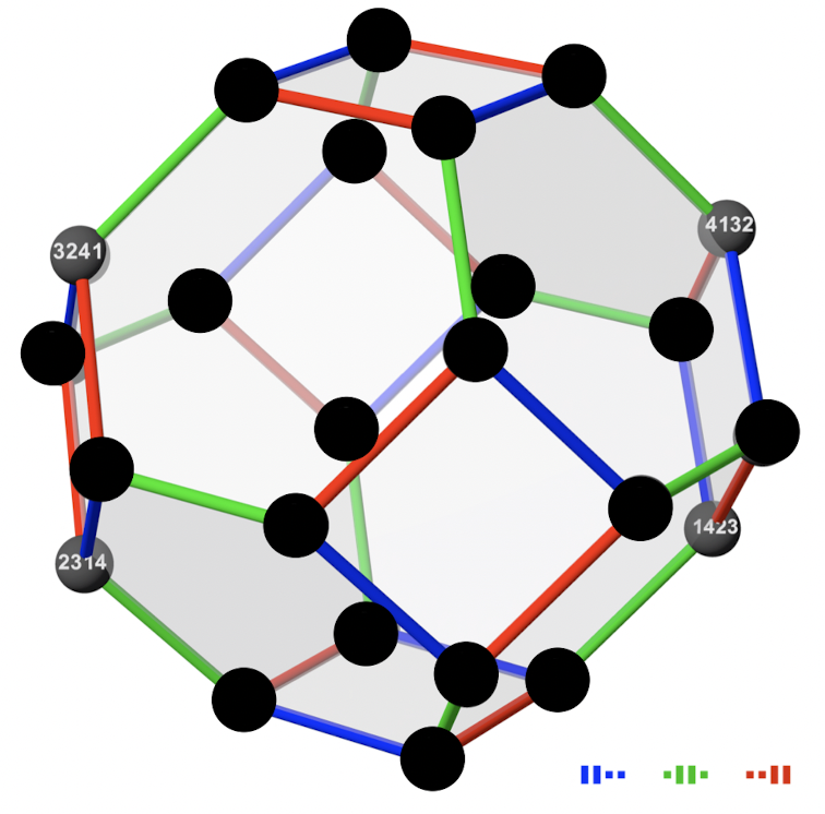
Figure 9: Elements of the Chiral multiplet. Starting at 1423, the hopping operators will generate the three other elements.

Similarly, for 4D $\cal N$=2 (dimensionally reduced to D=1, $\cal N$=8), we can generate all the elements of a supermultiplet given a single element and the hopping operators. For example, for the chiral-vector supermultiplet, starting with $\mathbf{L}^{CV}_{1}=(170)_{b}\langle 14236857\rangle$ (and focusing only on the permutation matrix component), we can act with the hopping operators

$$\begin{array}[]{llcl}\mathcal{P}_{1}=\mathbf{I}_{2}\otimes\mathbf{I}_{2}\otimes\mathbf{I}_{2}=&()&=&\langle 12345678\rangle\\ \mathcal{P}_{2}=\mathbf{I}_{2}\otimes\mathbf{I}_{2}\otimes\sigma^{1}=&(12)(34)(56)(78)&=&\langle 21436587\rangle\\ \mathcal{P}_{3}=\mathbf{I}_{2}\otimes\sigma^{1}\otimes\mathbf{I}_{2}=&(13)(24)(57)(68)&=&\langle 34127856\rangle\\ \mathcal{P}_{4}=\mathbf{I}_{2}\otimes\sigma^{1}\otimes\sigma^{1}=&(14)(23)(58)(67)&=&\langle 43218765\rangle\\ \mathcal{P}_{5}=\sigma^{1}\otimes\mathbf{I}_{2}\otimes\mathbf{I}_{2}=&(15)(26)(37)(48)&=&\langle 56781234\rangle\\ \mathcal{P}_{6}=\sigma^{1}\otimes\mathbf{I}_{2}\otimes\sigma^{1}=&(16)(25)(38)(47)&=&\langle 65872143\rangle\\ \mathcal{P}_{7}=\sigma^{1}\otimes\sigma^{1}\otimes\mathbf{I}_{2}=&(17)(28)(35)(46)&=&\langle 78563412\rangle\\ \mathcal{P}_{8}=\sigma^{1}\otimes\sigma^{1}\otimes\sigma^{1}=&(18)(27)(36)(45)&=&\langle 87654321\rangle\end{array}$$ (3.14)

in which case we can reproduce all elements of the chiral-vector supermultiplet as follows.

$$\mathcal{P}_{1}|\mathbf{L}^{CV}_{1}|=()\langle 14236857\rangle=\langle 14236857\rangle=|\mathbf{L}^{CV}_{1}|$$ (3.15)

$$\mathcal{P}_{2}|\mathbf{L}^{CV}_{1}|=(12)(34)(56)(78)\langle 14236857\rangle=\langle 23145768\rangle=|\mathbf{L}^{CV}_{2}|$$

$$\mathcal{P}_{3}|\mathbf{L}^{CV}_{1}|=(13)(24)(57)(68)\langle 14236857\rangle=\langle 32418675\rangle=|\mathbf{L}^{CV}_{3}|$$

$$\mathcal{P}_{4}|\mathbf{L}^{CV}_{1}|=(14)(23)(58)(67)\langle 14236857\rangle=\langle 41327586\rangle=|\mathbf{L}^{CV}_{4}|$$

$$\mathcal{P}_{5}|\mathbf{L}^{CV}_{1}|=(15)(26)(37)(48)\langle 14236857\rangle=\langle 58672413\rangle=|\mathbf{L}^{CV}_{5}|$$

$$\mathcal{P}_{6}|\mathbf{L}^{CV}_{1}|=(16)(25)(38)(47)\langle 14236857\rangle=\langle 67581324\rangle=|\mathbf{L}^{CV}_{6}|$$

$$\mathcal{P}_{7}|\mathbf{L}^{CV}_{1}|=(17)(28)(35)(46)\langle 14236857\rangle=\langle 76854231\rangle=|\mathbf{L}^{CV}_{7}|$$

$$\mathcal{P}_{8}|\mathbf{L}^{CV}_{1}|=(18)(27)(36)(45)\langle 14236857\rangle=\langle 85763142\rangle=|\mathbf{L}^{CV}_{8}|$$

3.3 Partitioning the Permutahedron via Cosets

It was found in  [?] that the partitioning of $S_{4}$ can be understood in terms of cosets of Klein’s Vierergruppe, i.e. the set

$$V=\{\langle 1234\rangle,\langle 2143\rangle,\langle 3412\rangle,\langle 4321\rangle\}.$$ (3.16)

The Vierergruppe is a normal subgroup of $S_{4}$, and it is isomorphic to the group $(Z_{2})^{\oplus 2}$.

Here, we define cosets and normal subgroups as follows:

Definition 1

Let $\mathcal{H}=\{h_{i}\}$ be a subgroup of $S_{n}$ and $g\in S_{n}$ be any group element. We call the set $g\mathcal{H}=\{gh_{i}\}$ the left coset by $g$, and the set $\mathcal{H}g=\{h_{i}g\}$ the right coset by $g$.

Definition 2

A subgroup $\mathcal{X}$ of the group $G$ is a normal subgroup of $G$ if and only if $g^{-1}xg\in\mathcal{X}$ for every $x\in\mathcal{X}$ and $g\in G$.

A consequence of this definition is that, if $\mathcal{X}$ is normal in $G$, left and right cosets of $\mathcal{X}$ are equivalent. That is, $\mathcal{X}g=g\mathcal{X},$ $\forall g\in G$.

In particular, each of the supermultiplets of $\cal N$=1 supersymmetry can be written as right cosets (or equivalently, left cosets, since $V$ is normal in $S_{4}$) of $V$:

$$VM_{3} =V$$ (3.17)

$$VM_{2} =V\langle 2134\rangle$$ (3.18)

$$VM_{1} =V\langle 3214\rangle$$ (3.19)

$$VM =V\langle 1324\rangle$$ (3.20)

$$CM =V\langle 2314\rangle$$ (3.21)

$$TM =V\langle 3124\rangle.$$ (3.22)

When applied to the permutahedron, we recall findings regarding the magic number rules within and between these sets  [?]. With a suitable choice of sign prefactors, the Vierergruppe and its cosets form valid garden algebras.

Returning to  [?], the authors note that using the analogue of the Vierergruppe in $S_{8}$, the same partitioning can be accomplished. We can construct this analogue, which we call the Rana subgroup $\mathcal{R}_{8}$, by following the method outlined in Sec. 2, starting with the Vierergruppe. The result is

$$\mathcal{R}_{8}=\{ \langle 12345678\rangle,\langle 21436587\rangle,\langle 34127856\rangle,\langle 43218765\rangle,$$ (3.23)

$$\langle 56781234\rangle,\langle 65872143\rangle,\langle 78563412\rangle,\langle 87654321\rangle\}.$$

This $\cal N$=2 supermultiplet is also identified in  [?] and is isomorphic to the group $(Z_{2})^{\oplus 3}$. As $\mathcal{R}_{8}$ forms a subgroup of $S_{8}$, its cosets will partition $S_{8}$ into octets. However, in contrast with the Vierergruppe in $S_{4}$, $\mathcal{R}_{8}$ is not normal in $S_{8}$, so taking left and right cosets will not necessarily yield the same partitions. Indeed, there are 30 conjugate subgroups of $\mathcal{R}_{8}$ that, when cosets are taken, will each yield a separate partition of $S_{8}$  [?]. The chiral-chiral, chiral-vector, and chiral-tensor supermultiplets are right cosets of $\mathcal{R}_{8}$. See Sec. 3.2 for an explicit construction of the chiral-vector supermultiplet by this method. Again, with suitable choices of sign prefactors, $\mathcal{R}_{8}$, its conjugates, and their cosets for valid garden algebras.

We can further employ this method to generate a partition of $S_{16}$ via a recursive construction of the Rana subgroup (here, we must delineate terms of a permutation with commas to avoid ambiguity):

$$\mathcal{R}_{16}=\{ \langle 1,2,3,4,5,6,7,8,9,10,11,12,13,14,15,16\rangle,\langle 2,1,4,3,6,5,8,7,10,9,12,11,14,13,16,15\rangle,$$ (3.24)

$$\langle 3,4,1,2,7,8,5,6,11,12,9,10,15,16,13,14\rangle,\langle 4,3,2,1,8,7,6,5,12,11,10,9,16,15,14,13\rangle,$$

$$\langle 5,6,7,8,1,2,3,4,13,14,15,16,9,10,11,12\rangle,\langle 6,5,8,7,2,1,4,3,14,13,16,15,10,9,12,11\rangle,$$

$$\langle 7,8,5,6,3,4,1,2,15,16,13,14,11,12,9,10\rangle,\langle 8,7,6,5,4,3,2,1,16,15,14,13,12,11,10,9\rangle,$$

$$\langle 9,10,11,12,13,14,15,16,1,2,3,4,5,6,7,8\rangle,\langle 10,9,12,11,14,13,16,15,2,1,4,3,6,5,8,7\rangle,$$

$$\langle 11,12,9,10,15,16,13,14,3,4,1,2,7,8,5,6\rangle,\langle 12,11,10,9,16,15,14,13,4,3,2,1,8,7,6,5\rangle,$$

$$\langle 13,14,15,16,9,10,11,12,5,6,7,8,1,2,3,4\rangle,\langle 14,13,16,15,10,9,12,11,6,5,8,7,2,1,4,3\rangle,$$

$$\langle 15,16,13,14,11,12,9,10,7,8,5,6,3,4,1,2\rangle,\langle 16,15,14,13,12,11,10,9,8,7,6,5,4,3,2,1\rangle\}.$$

We once again note that $\mathcal{R}_{16}$ is isomorphic to $(Z_{2})^{\oplus 4}$, and it is a subgroup of $S_{16}$ (though not a normal subgroup). Thus, the set forms two separate partitions of $S_{16}$: that formed by left cosets, and that formed by right cosets. However, in contrast with previous cases, we find by direct search that there is no suitable choice of signs to convert $\mathcal{R}_{16}$ into a garden algebra. The results in  [?] indicate that we may have to go as far as $S_{128}$ to find a valid $N=16$ garden algebra. The reason for this breach of pattern we leave for future exploration.

3.4 The magic number

In  [?], the idea of a number (hereafter called “the magic number”) that constrains the “positions” of elements within a supermultiplet relative to the rest of the permutahedron was introduced. The magic number intriguingly refers to two different but equivalent notions: the intra-tet correlator, and the inter-tet correlator. (These were originally dubbed “intra-quartet” and “inter-quartet” correlators, as they were studied in the context of $\cal N$=4 supersymmetry.) First, the intra-tet correlator of a given supermultiplet $\mathcal{A}$ and element $\pi\in\mathcal{A}$, labeled $\rm{Intra}_{\pi}(\mathcal{A})$, is the sum of the distances between $\pi$ and each other element of $\mathcal{A}$; that is,

$$\rm{Intra}_{\pi}(\mathcal{A})=\sum_{\alpha\in\mathcal{A}}d(\pi,\alpha),$$ (3.25)

where $\rm d(\cdot,\cdot)$ is the hamming or Bruhat distance function detailed in  [?]. Second, the inter-tet correlator of a given permutation $\pi\in\mathcal{A}$ to a supermultiplet $\mathcal{B}\neq\mathcal{A}$, labeled $\rm{Inter}_{\pi}(\mathcal{A},\mathcal{B})$ is the sum of the distances between $\pi$ and each element of $\mathcal{B}$; that is,

$$\rm{Inter}_{\pi}(\mathcal{A},\mathcal{B})=\sum_{\beta\in\mathcal{B}}d(\pi,\beta).$$ (3.26)

What is remarkable about these quantities, and what in fact merits their collective description as the magic number, is that, in both $S_{4}$ and $S_{8}$, for any supermultiplets $\mathcal{A},\mathcal{B}$ and any elements $\pi,\sigma\in\mathcal{A}$,

$$\rm{Intra}_{\pi}(\mathcal{A})=\rm{Intra}_{\sigma}(\mathcal{A})=\rm{Inter}_{\pi}(\mathcal{A},\mathcal{B})=\rm{Inter}_{\sigma}(\mathcal{A},\mathcal{B}).$$ (3.27)

In $S_{4}$ and $S_{8}$, this has been confirmed by brute force calculation, the magic number in $S_{4}$ being 12 and in $S_{8}$ being 112. In $S_{16}$, $\rm{Intra}_{\langle 1,2,3,4,5,6,7,8,9,10,11,12,13,14,15,16\rangle}(\mathcal{R}_{16})=960$, though the sheer size of $S_{16}$ has precluded a full validation of the identity (3.27). We conjecture that this magic number rule will hold for partitions in arbitrary $S_{2^{n}}$, the magic number being ${\cal G}_{(3)}=$$2^{2n-2}(2^{n}-1)$.

Notice that for a permutahedron of dimension $D$, the average distance between two vertices would be $(D-1)D/4$, which can be proved by induction. When $D=2^{n}$ and there are $D$ vertices in a multiplet, we can then approximate the magic number by the average distance

$$(D-1)D/4\times D=(2^{n}-1)2^{2n}/4=2^{2n-2}(2^{n}-1)$$ (3.28)

which exactly matches with our conjectured magic number.

Future work may focus on the theoretical grounding for this magic number rule, while the rule itself may function as a crucial technique for the validation of supermultiplets.

4 The Appearance of Ab-normal Cosets in BC(8)

We have seen in Sec. 3.3 that, in the 4D $\mathcal{N}=1$ case, left and right cosets are equivalent for purposes of partitioning the permutahedron, but in the 4D $\mathcal{N}=2$ case, they are not. Here, we investigate some consequences of this fact.

4.1 4D $\mathcal{N}=1$ ab-normal coset

Let us first explicitly calculate left and right cosets for the 4D $\mathcal{N}=1$ case using the Vierergruppe $VM_{3}$ as the set of hopping operators. This set has also been dubbed the diadem set $O$  [?]. Also the diadem $O$ is the same as the object called Rana subgroup $\mathcal{R}_{n}$ in Sec. 3.3. We calculate the left- and right-cosets of 4D $\mathcal{N}=1$ case by $O$ with every element of $S_{4}$. Using Def. 1, we calculate the left and right cosets of $O$ by elements in $S_{4}$. As expected, we find six distinct cosets. Table. LABEL:tab01 and LABEL:tab02 shows the left- and right-coset list for 4D $\mathcal{N}=1$ case.

Table 1: $S_{4}$ left-cosets list

No.	Element 1	Element 2	Element 3	Element 4	Type
1	1234	2143	3412	4321	$O$/$VM_{3}$
2	1243	2134	3421	4312	$VM_{2}$
3	1324	2413	3142	4231	$VM$
4	1342	2431	3124	4213	$TM$
5	1423	2314	3241	4132	$CM$
6	1432	2341	3214	4123	$\rm VM_{1}$

Table 2: $S_{4}$ right-cosets list

No.	Element 1	Element 2	Element 3	Element 4	Type
1	1234	2143	3412	4321	$O$/$VM_{3}$
2	1243	2134	4312	3421	$VM_{2}$
3	1324	3142	2413	4231	$VM$
4	1342	3124	4213	2431	$TM$
5	1423	4132	2314	3241	$CM$
6	1432	4123	3214	2341	$VM_{1}$

Here, we write 1234 to mean the permutation $\langle 1234\rangle$ for convinience. Also, we call each row of Table LABEL:tab01 and Table LABEL:tab02 a Kevin’s Pizza slice. Kevin’s Pizza refers to a partitioning of the permutation group of order four  [?] (as in Fig. 1). Table LABEL:tab01 and Table LABEL:tab02 show that although the Vierergruppe generates identical left and right cosets, the order in which these elements occur changes. For example, the third row of Table LABEL:tab01 and Table LABEL:tab02 contain the same set elements but have different orders. To describe this particular mathematical property, we define

Definition 3

Let $O$ be a diadem of $S_{n}$, and let ${\rm KP}_{i}^{(n)}$ be the $i$-th slice of Kevin’s Pizza on $S_{n}$. If $Og=gO$ $\forall g\in{\rm KP}_{i}^{(n)}$, then we call ${\rm KP}_{i}^{(n)}$ an ab-normal coset.

Here the $i$-th slice of Kevin’s Pizza on $S_{n}$ is defined as

$${\rm KP}_{i}^{(n)}=Og_{i},$$ (4.1)

where $O$ is a diadem of $S_{n}$.

where the diadem $O$ is Rana subgroup $\mathcal{R}_{n}$ defined in Sec. 3.2-3.3 and $g_{i}$ is the $i$-th element in $S_{n}$ (weighted by the BK-map).

Based on Def. 3, in the $S_{4}$ case, we can say that all of the Kevin’s pizza slices are ab-normal cosets.

4.2 Left versus right hoppers

In $S_{8}$, using the set $\mathcal{R}_{8}$, explicit construction of the left- and right-hoppers yields

Table 3: Left Hoppers in 4D $\mathcal{N}=2$

Left Hoppers	Element1	Element2	Element3	Element4	Element5	Element6	Element7	Element8
$CMCM$	12345678	21436587	34127856	43218765	56781234	65872143	78563412	87654321
$CMTM$	12345678	21436587	34127856	43218765	56781234	65872143	78563412	87654321
$CMVM$	12345678	21436587	34127856	43218765	56781234	65872143	78563412	87654321
$TMVM$	12345678	21436587	34127856	43218765	56781234	65872143	78563412	87654321
$TMTM$	12345678	21436587	34127856	43218765	56781234	65872143	78563412	87654321
$VMVM$	12345678	21436587	34127856	43218765	56781234	65872143	78563412	87654321
$O$	12345678	21436587	34127856	43218765	56781234	65872143	78563412	87654321

Table 4: Right Hoppers in 4D $\mathcal{N}=2$

Right Hoppers	Element1	Element2	Element3	Element4	Element5	Element6	Element7	Element8
$CMCM$	12345678	34127856	43218765	21436587	56781234	78563412	87654321	65872143
$CMTM$	12345678	34128765	43216587	21437856	57861423	86573241	68754132	75682314
$CMVM$	12345678	34127856	43216587	21438765	76583214	58761432	85672341	67854123
$TMVM$	12345678	43217856	21436587	34128765	78654312	56871243	87563421	65782134
$TMTM$	12345678	43218765	21436587	34127856	56781234	87654321	65872143	78563412
$VMVM$	12345678	34127856	21436587	43218765	56781234	78563412	65872143	87654321
$O$	12345678	21436587	34127856	43218765	56781234	65872143	78563412	87654321

Here $CM$, $TM$, $VM$ are chiral-, tensor-, vector-multiplets defined from (2.7), (2.8), (2.9) and $CMCM$ is same as $(CC)$ which is the chiral-chiral $\mathcal{N}=2$ supermultiplet generated from concatenating two copies of the $\mathcal{N}=1$ supermultiplet in Sec. 2.1. And one can observe that in general the left and right hoppers of $CMCM$, $VMVM$, $TMTM$, and $O$ have a different ordering of elements, however, when taken as a set they are the same. This shows that there is an ab-normal coset in which the left and right cosets are the same as a set at 4D $\mathcal{N}=2$ case, which we can do a 0-brane reduction on 8D $\mathcal{N}=1$ (Eight color) case.

4.3 Eight color ab-normal coset

In general for the group $S_{n}$, we have  [?]:

Theorem 4

Let n $\geq$ 5. Then the only normal subgroups of $S_{n}$ are {()}, $A_{n}$, and $S_{n}$.

Here $A_{n}$ is the alternating group: the group of even permutations on a set of length $n$. Therefore, from $n\geq 5$, the diadem $O$ is not a normal subgroup of $S_{n}$.

In 4D $\mathcal{N}=2$ case, which is equivalent to 8D $\mathcal{N}=1$ after a 0-brane reduction we constructed the 8-th Extended Kevin’s Pizza using a diadem $O$ (Rana subgroup $\mathcal{R}_{8}$). Thus the total number of 8D $\mathcal{N}=1$ 8-th Extended Kevin’s Pizza slices are 7!=5040 because one 8-th Extended Kevin’s Pizza slice has 8 elements.

Then for every $g\in{\rm{KP}}_{i}^{(n)}$, $n=8$, we have

$$g{\mathcal{H}^{(R)}={\rm KP}_{i}^{(n)}},\quad{\mathcal{H}^{(L)}}g={\rm KP}_{i}^{(n)},$$ (4.2)

$${\rm\mathcal{H}^{(R)}=\{\mathcal{H}_{1}^{(R)},\mathcal{H}_{2}^{(R)},...,\mathcal{H}_{8}^{(R)}}\},\quad{\rm\mathcal{H}^{(L)}}=\{\mathcal{H}_{1}^{(L)},\mathcal{H}_{2}^{(L)},...,\mathcal{H}_{8}^{(L)}\}.$$ (4.3)

Here $\rm\mathcal{H}_{A}^{(L)}$, $\rm\mathcal{H}_{A}^{(R)}$ are defined in (3.4).

And when $\mathcal{H}^{(L)}$ and $\mathcal{H}^{(R)}$ are the same, we find

$${\rm\mathcal{H}^{(L)}}g=g{\rm\mathcal{H}^{(L)}}={\rm KP}_{i}^{(n)}.$$ (4.4)

By using (4.1) and (4.4),

$${\rm\mathcal{H}^{(L)}}={O}$$ (4.5)

Therefore, if there is any ${\rm KP}_{i}^{(n)}$ which has the same left- and right-hoppers simultaneously, then from (4.4), (4.5) and Def. 3 we can call this kind of $n$-th extended Kevin’s Pizza slice an ab-normal coset.

In the appendix, Table. LABEL:tab5 shows the ab-normal coset list on eight color case with the lexicographic order (BK-map) from $\langle 12345678\rangle$ to $\langle 18726345\rangle$. As a result, one can see there are 168 sets in which the set of left- and right-hoppers are the same, which means each 8-th extended Kevin’s Pizza slices on the list is an ab-normal coset. And the highlighted rows’ elements of Table. LABEL:tab5 have (4D $\mathcal{N}=1$ supermultiplet)+(4D $\mathcal{N}=1$ supermultiplet) decomposable structures, such as $VMVM$. And from row 72, the highlighted row patterns are based on the repetition of the first 24 rows, but it does not have particular type naming compared to 4D $\mathcal{N}=1$ supermultiplet.

Thus, in further investigation, one need is to clarify why the highlighted supermultiplet type consists of the same copies of 4D $\mathcal{N}=1$ supermultiplet such as (CC), (VV), (TT) rather than different combinations, eg., (CT), (CV), (VT), and why there is particular number (168) of ab-normal cosets which exists in 4D $\mathcal{N}=2$.

5 Towards a Polytopic Representation Theory for Supersymmetry

In our previous work  [?], we discussed the potential to view faces of the permutahedron as being composed of valid supermultiplets of a lower degree. In fact, we can realize this by examining how $\cal N$=3 permutahedra (hexagons) conspire to create the $\cal N$=4 permutahedron (truncated octahedron). In Fig. 10 and Fig. 11, the construction of an $\cal N$=4 permutahedron out of $\cal N$=3 permutahedra is demonstrated. We start by taking the three element string “123” and using bruhat weak ordering to create two hexagons. Then, we add a “4” to the left hand side of all elements of one hexagon, and a “4” to the right hand side of all elements of the other hexagon. Fig. 10 shows how this pair of hexagons fits on the completed $\cal N$=4 permutahedron. By following this construction for three more pairs of hexagons, where the respective added element is a “1”, “2”, and “3” (as depicted in Fig. 11), we can complete the construction of the $\cal N$=4 permutahedron. The square faces (which in our previous work  [?] were identified as supermultiplets of a lower degree or extension) are seen to arise as a consequence of creating the pairs of hexagonal faces.

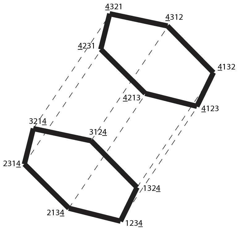
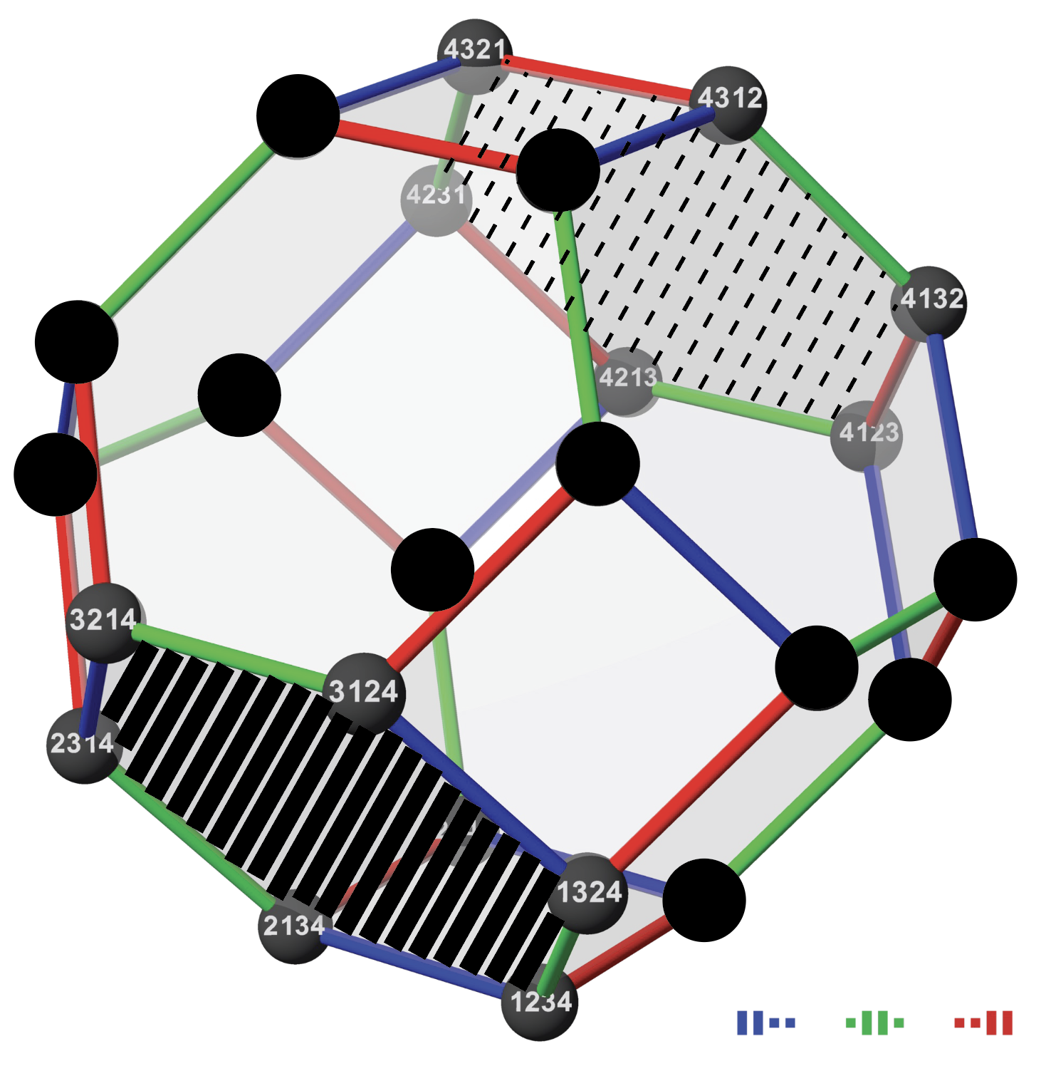
Figure 10: Illustration of the hexagon pair and its position on the 3rd order permutahedron

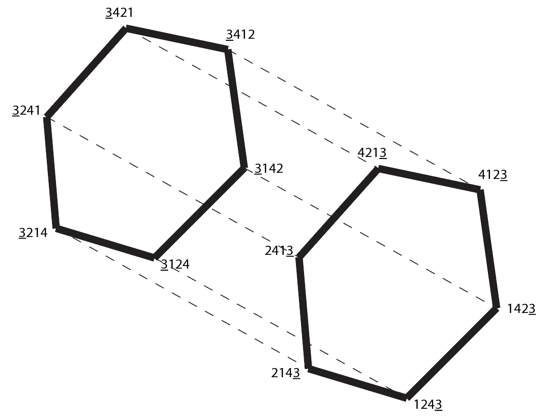
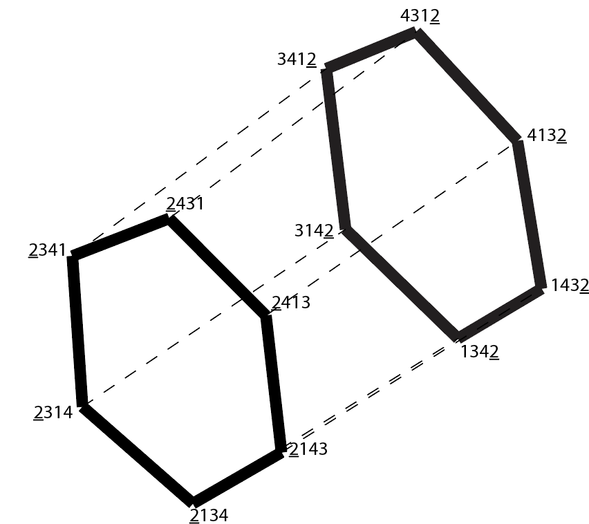
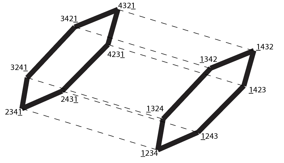
Figure 11: Illustration of the four hexagon pairs that generate the 3rd order permutahedron

A similar construction may be carried out for higher $\cal N$ permutahedra. For example, the permutahedra of order 5, the omnitruncated 5-cell, depicted in Fig. 12. This permutahedra is composed of 10 truncated octahedra, and 20 hexagonal prisms. If we were to carry out the analogous construction as for the $\cal N$=4 permutahedra, we would find that the truncated octahedra being put together would make the hexagonal prisms similarly emergent as the square faces were in the $\cal N$=4 case. This is strongly suggestive that our approach of creating higher degree supermultiplets out of lower degree supermultiplets is mathematically robust. Creating higher order supermultiplets out of lower order supermultiplets can be reduced to a problem of identifying vertices on a permutahedron of higher degree.

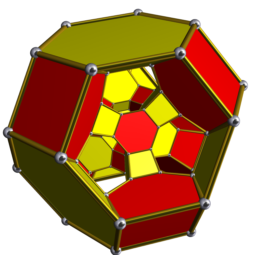
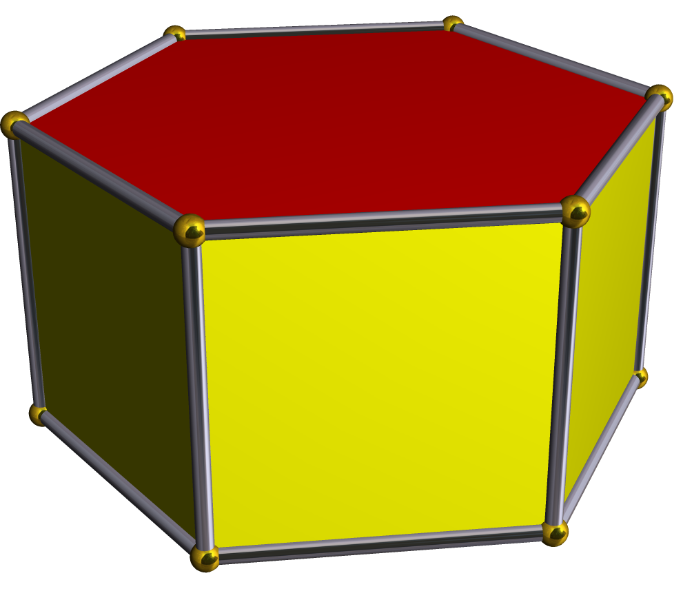
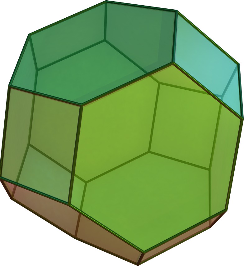
Figure 12: The omnitruncated 5-cell, constructed from truncated octahedra and hexagonal prisms

It’s notable that the types of 2-faces remain the same even as $\cal N$ scales. This isn’t true for any of the other types of faces we examined (up to 5-faces).

Types of 2-faces
$\cal{N}$	{4}	{6}
3	0	1
4	6	8
5	90	60
6	1080	480
7	12600	4200
8	151200	40320

Types of 3-faces
$\cal{N}$	{8}	{12}	{24}
4	0	0	1
5	0	20	10
6	90	360	90
7	2520	5040	840
8	50400	67200	8400

Types of 4-faces
$\cal{N}$	{16}	{24}	{36}	{48}	{120}
5	0	0	0	0	1
6	0	0	20	30	12
7	0	630	420	630	126
8	2520	20160	6720	10080	1344

Types of 5-faces
$\cal{N}$	{72}	{96}	{144}	{240}	{720}
6	0	0	0	0	1
7	0	0	70	42	14
8	1680	1260	1680	1008	168

Types of 6-faces
$\cal{N}$	{72}	{96}	{144}	{240}
7	0	0	0	1
8	70	112	56	16

6 Conclusions and Summary

In this work, we have begun the exploration of the permutahedron associated with the omnitruncated 7-simplex. With regard to supersymmetry, this is the appropriate setting for models where eight independent supercharges occur.

In Sec. 1, we reviewed past works and brought a new perspective to them. We began our presentation by reviewing some “traditional” color problems of mathematics such as the four color map problem and the Graph Vertex Coloring Problem. The latter can be considered in the case where the polytope is the truncated octahedron. This polytope occurs in the structure of the permutahedron associated with the permutation group of order four, $\{{\mathbb{S}}{}_{4}\}$. We also noted in Fig. 3 that Clifford Algebra matrices are associated with the color-coded permutation matrices. While we did not mention it in Sec. 1.1, that pattern is also a solution to the Graph Coloring Vertex Problem!

An examination of that image shows that no edge is connected to two vertices associated with the same color. This is true of the square faces, and it is also true for the hexagonal faces! So adinkras, which have adjacency matrices that form Clifford Algebras, in the cases under study can be associated with solutions of the ‘traditional’ Graph Vertex Coloring Problem. Should this hold in general, the emergence of SUSY via graph theory, would be intimately connected with the “traditional” Graph Vertex Coloring Problem. This is one of the most suggestive, and perhaps important, realization presented in the current work!

In Sec. 2, the focus was on how previously uncovered adinkras and associated Clifford Algebras in the case of four colors, can be as a starting to construct the similar adinkras and associated Clifford Algebras in the case of eight colors. We demonstrated a set of constructive rules that accomplish this goal.

In Sec. 3, the challenge of uncovering operators that play the role of raising operators in compact Lie Algebras (or alternating as “hopping operator” in systems of lattices in physics problems) for the space of adinkras was considered. Although the Jordan-Chevelley Decomposition of the generators in Lie algebras appear not to apply, in any obvious fashion, due to the appearance of permutation matrices, a concept that induces a weighted ordering can be obtained from another viewpoint. As noted in equations (3.2) and (3.3), there is a natural notion of the weight of permutation matrices that is induced by a map from the action of the permutation matrices on their carrier spaces into the real numbers. This notion of ordering is actually implicit in the results that follow from Bruhat ordering. Using these concepts, we constructed elementary left hopping and right hopping operators which have the effect of generating translation on the space of the permutahedron. These were given for both the cases of four-color and eight-color systems.

This same section also formally introduced the concept of the “magic number.” In the first chapter, a verbal description of it was given and as well the symbol ${\cal G}{}_{(3)}$ was introduced for this quantity. In equations (3.25) and (3.26) two formal mathematical definitions have been presented to precisely define the values of ${\cal G}{}_{(3)}$. For the cases of $\{{\mathbb{S}}{}_{4}\}$, $\{{\mathbb{S}}{}_{8}\}$, and $\{{\mathbb{S}}{}_{16}\}$, our studies indicate the results shown in Table. LABEL:tab06

Table 5: $S_{4}$ left-coset

${\cal G}{}_{(3)}$-Value	Permutation Group
12	${~{}~{}~{}~{}~{}~{}~{}~{}~{}~{}~{}}\{{\mathbb{S}}{}_{4}\}$
112	${~{}~{}~{}~{}~{}~{}~{}~{}~{}~{}~{}}\{{\mathbb{S}}{}_{8}\}$
960	${~{}~{}~{}~{}~{}~{}~{}~{}~{}~{}~{}}\{{\mathbb{S}}{}_{16}\}$

and we conjecture the formula in equation (3.28) will hold for the special cases of $\{{\mathbb{S}}{}_{2^{r}}\}$.

In Sec. 4 we report on a new phenomenon. For the case of $\{{\mathbb{S}}{}_{4}\}$ the left hoppers and the right hoppers are one and the same when considered as unordered sets. This is due to the fact that the quartets that appear are cosets of $\{{\mathbb{S}}{}_{4}\}$ with respect to the Klein Group and the latter is a normal subgroup in forming these cosets. In the case of $\{{\mathbb{S}}{}_{8}\}$ we are no longer dealing with a normal subgroup. But remarkably enough when one looks at sets instead of individual elements, there are one-hundred and sixty-eight subsets that act as if they are normal groups. We have given the name ‘ab-normal’ to these sets. In further investigations, we can do more analysis on how many ab-normal cosets appear in more high-order dimensions.

Finally, in Sec. 5 we investigated the $k$-face analysis of higher-order permutahedron. We constructed a method to build 4-order permutahedron from 2D hexagon pairs. The $k$-face analysis yields the polytopic way to construct higher-degree supermultiplets out of lower-degree supermultiplets. By using the computer simulation, we obtain the partial $k$-face spectrum up to $\mathcal{N}=8$ and $k=5$. In further investigations, we can do more analysis on how many numbers of $k$-face type exists on particular $\mathcal{N}$-order permutahedron.

Let us end by making a comment about a new possible restriction that is revealed by the current work. We can refer to this as the ‘restriction of decomposability.’

In the case of the four color case, there were found to be six subsets of the permutation group $\{{\mathbb{S}}{}_{4}\}$, embedded within the Coxeter Group, that led to 1D, $N$ = 4 supermultiplets, i.e. provide the basis for Clfford Algebras. Thus, if one begins with these six subsets as a starting point to construct 1D, $N$ = 8 off-shell supermultiplets in pairs, then the experience of the work in  [?] informs us that each member of the pairs must be chosen to be distinct. So there must be 6 $\times$ 5 = 30 such pairings as the basis to construct 1D, $N$ = 8 off-shell supermultiplets that are decomposable! It is notable that the number 30 has also appeared in one of our previous investigations  [?]. Whether these occurrences are simply the result of accidents is a topic for future study. This observation has the potential to imposed drastic reductions in the space of acceptable ${{\boldsymbol{{\rm L}}}}{}_{{}_{{\rm I}}}$-${{\boldsymbol{{\rm R}}}}{}_{{}_{{\rm I}}}$ collections.

“Behind it all is surely an idea so simple, so beautiful,     that when we grasp it - in a decade, a century, or a    millennium - we will all say to each other, how could it have been otherwise? How could we have been so stupid?”
 
    -   John Archibald Wheeler

Acknowledgements

We wish to acknowledge conversation with Dr. D. E. A. Gates for useful comments on this work. The research of S. J. G., A. C.  and Z. Z. was supported during a portion of the time it was carried out by the endowment of the Ford Foundation Professorship of Physics at Brown University. All also gratefully acknowledge the support of the Brown Theoretical Physics Center. In addition, the research of S. J. G. is supported by the Clark Leadership Chair in Science endowment at the University of Maryland - College Park.

7 Appendix

7.1 Eight color ab-normal cosets

Table 6: Eight color ab-normal cosets list

No.	Element1	Element2	Element3	Element4	Element5	Element6	Element7	Element8	Type
1	12345678	21436587	34127856	43218765	56781234	65872143	78563412	87654321	O/$\rm VM_{3}VM_{3}$
2	12346587	21435678	34128765	43217856	56782143	65871234	78564321	87653412
3	12347856	21438765	34125678	43216587	56783412	65874321	78561234	87652143
4	12348765	21437856	34126587	43215678	56784321	65873412	78562143	87651234
5	12435687	21346578	34217865	43128756	56871243	65782134	78653421	87564312	$\rm VM_{2}VM_{2}$
6	12436578	21345687	34218756	43127865	56872134	65781243	78654312	87563421
7	12437865	21348756	34215687	43126578	56873421	65784312	78651243	87562134
8	12438756	21347865	34216578	43125687	56874312	65783421	78652134	87561243
9	12563478	21654387	34781256	43872165	56127834	65218743	78345612	87436521
10	12564387	21653478	34782165	43871256	56128743	65217834	78346521	87435612
11	12567834	21658743	34785612	43876521	56123478	65214387	78341256	87432165
12	12568743	21657834	34786521	43875612	56124387	65213478	78342165	87431256
13	12653487	21564378	34871265	43782156	56217843	65128734	78435621	87346512
14	12654378	21563487	34872156	43781265	56218734	65127843	78436512	87345621
15	12657843	21568734	34875621	43786512	56213487	65124378	78431265	87342156
16	12658734	21567843	34876512	43785621	56214378	65123487	78432156	87341265
17	12783456	21874365	34561278	43652187	56347812	65438721	78125634	87216543
18	12784365	21873456	34562187	43651278	56348721	65437812	78126543	87215634
19	12785634	21876543	34567812	43658721	56341278	65432187	78123456	87214365
20	12786543	21875634	34568721	43657812	56342187	65431278	78124365	87213456
21	12873465	21784356	34651287	43562178	56437821	65348712	78215643	87126534
22	12874356	21783465	34652178	43561287	56438712	65347821	78216534	87125643
23	12875643	21786534	34657821	43568712	56431287	65342178	78213465	87124356
24	12876534	21785643	34658712	43567821	56432178	65341287	78214356	87123465
25	13245768	24136857	31427586	42318675	57681324	68572413	75863142	86754231	$\rm VMVM$
26	13246857	24135768	31428675	42317586	57682413	68571324	75864231	86753142
27	13247586	24138675	31425768	42316857	57683142	68574231	75861324	86752413
28	13248675	24137586	31426857	42315768	57684231	68573142	75862413	86751324
29	13425786	24316875	31247568	42138657	57861342	68752431	75683124	86574213	$\rm TMTM$
30	13426875	24315786	31248657	42137568	57862431	68751342	75684213	86573124
31	13427568	24318657	31245786	42136875	57863124	68754213	75681342	86572431
32	13428657	24317568	31246875	42135786	57864213	68753124	75682431	86571342
33	13572468	24681357	31754286	42863175	57136824	68245713	75318642	86427531
34	13574286	24683175	31752468	42861357	57138642	68247531	75316824	86425713
35	13576824	24685713	31758642	42867531	57132468	68241357	75314286	86423175
36	13578642	24687531	31756824	42865713	57134286	68243175	75312468	86421357
37	13682457	24571368	31864275	42753186	57246813	68135724	75428631	86317542
38	13684275	24573186	31862457	42751368	57248631	68137542	75426813	86315724
39	13685724	24576813	31867542	42758631	57241368	68132457	75423186	86314275
40	13687542	24578631	31865724	42756813	57243186	68134275	75421368	86312457
41	13752486	24861375	31574268	42683157	57316842	68425731	75138624	86247513
42	13754268	24863157	31572486	42681375	57318624	68427513	75136842	86245731
43	13756842	24865731	31578624	42687513	57312486	68421375	75134268	86243157
44	13758624	24867513	31576842	42685731	57314268	68423157	75132486	86241375
45	13862475	24751386	31684257	42573168	57426831	68315742	75248613	86137524
46	13864257	24753168	31682475	42571386	57428613	68317524	75246831	86135742
47	13865742	24756831	31687524	42578613	57421386	68312475	75243168	86134257
48	13867524	24758613	31685742	42576831	57423168	68314257	75241386	86132475
49	14235867	23146758	32417685	41328576	58671423	67582314	76853241	85764132	$\rm CMCM$
50	14236758	23145867	32418576	41327685	58672314	67581423	76854132	85763241
51	14237685	23148576	32415867	41326758	58673241	67584132	76851423	85762314
52	14238576	23147685	32416758	41325867	58674132	67583241	76852314	85761423
53	14325876	23416785	32147658	41238567	58761432	67852341	76583214	85674123	$\rm VM_{1}VM_{1}$
54	14326785	23415876	32148567	41237658	58762341	67851432	76584123	85673214
55	14327658	23418567	32145876	41236785	58763214	67854123	76581432	85672341
56	14328567	23417658	32146785	41235876	58764123	67853214	76582341	85671432
57	14582367	23671458	32764185	41853276	58146723	67235814	76328541	85417632
58	14583276	23674185	32761458	41852367	58147632	67238541	76325814	85416723
59	14586723	23675814	32768541	41857632	58142367	67231458	76324185	85413276
60	14587632	23678541	32765814	41856723	58143276	67234185	76321458	85412367
61	14672358	23581467	32854176	41763285	58236714	67145823	76418532	85327641
62	14673285	23584176	32851467	41762358	58237641	67148532	76415823	85326714
63	14675823	23586714	32857641	41768532	58231467	67142358	76413285	85324176
64	14678532	23587641	32856714	41765823	58234176	67143285	76412358	85321467
65	14762385	23851476	32584167	41673258	58326741	67415832	76148523	85237614
66	14763258	23854167	32581476	41672385	58327614	67418523	76145832	85236741
67	14765832	23856741	32587614	41678523	58321476	67412385	76143258	85234167
68	14768523	23857614	32586741	41675832	58324167	67413258	76142385	85231476
69	14852376	23761485	32674158	41583267	58416732	67325841	76238514	85147623
70	14853267	23764158	32671485	41582376	58417623	67328514	76235841	85146732
71	14856732	23765841	32678514	41587623	58412376	67321485	76234158	85143267
72	14857623	23768514	32675841	41586732	58413267	67324158	76231485	85142376
73	15263748	26154837	37481526	48372615	51627384	62518473	73845162	84736251
74	15264837	26153748	37482615	48371526	51628473	62517384	73846251	84735162
75	15267384	26158473	37485162	48376251	51623748	62514837	73841526	84732615
76	15268473	26157384	37486251	48375162	51624837	62513748	73842615	84731526
77	15372648	26481537	37154826	48263715	51736284	62845173	73518462	84627351
78	15374826	26483715	37152648	48261537	51738462	62847351	73516284	84625173
79	15376284	26485173	37158462	48267351	51732648	62841537	73514826	84623715
80	15378462	26487351	37156284	48265173	51734826	62843715	73512648	84621537
81	15482637	26371548	37264815	48153726	51846273	62735184	73628451	84517362
82	15483726	26374815	37261548	48152637	51847362	62738451	73625184	84516273
83	15486273	26375184	37268451	48157362	51842637	62731548	73624815	84513726
84	15487362	26378451	37265184	48156273	51843726	62734815	73621548	84512637
85	15623784	26514873	37841562	48732651	51267348	62158437	73485126	84376215
86	15624873	26513784	37842651	48731562	51268437	62157348	73486215	84375126
87	15627348	26518437	37845126	48736215	51263784	62154873	73481562	84372651
88	15628437	26517348	37846215	48735126	51264873	62153784	73482651	84371562
89	15732684	26841573	37514862	48623751	51376248	62485137	73158426	84267315
90	15734862	26843751	37512684	48621573	51378426	62487315	73156248	84265137
91	15736248	26845137	37518426	48627315	51372684	62481573	73154862	84263751
92	15738426	26847315	37516248	48625137	51374862	62483751	73152684	84261573
93	15842673	26731584	37624851	48513762	51486237	62375148	73268415	84157326
94	15843762	26734851	37621584	48512673	51487326	62378415	73265148	84156237
95	15846237	26735148	37628415	48517326	51482673	62371584	73264851	84153762
96	15847326	26738415	37625148	48516237	51483762	62374851	73261584	84152673
97	16253847	25164738	38471625	47382516	52617483	61528374	74835261	83746152
98	16254738	25163847	38472516	47381625	52618374	61527483	74836152	83745261
99	16257483	25168374	38475261	47386152	52613847	61524738	74831625	83742516
100	16258374	25167483	38476152	47385261	52614738	61523847	74832516	83741625
101	16382547	25471638	38164725	47253816	52746183	61835274	74528361	83617452
102	16384725	25473816	38162547	47251638	52748361	61837452	74526183	83615274
103	16385274	25476183	38167452	47258361	52741638	61832547	74523816	83614725
104	16387452	25478361	38165274	47256183	52743816	61834725	74521638	83612547
105	16472538	25381647	38254716	47163825	52836174	61745283	74618352	83527461
106	16473825	25384716	38251647	47162538	52837461	61748352	74615283	83526174
107	16475283	25386174	38257461	47168352	52831647	61742538	74613825	83524716
108	16478352	25387461	38256174	47165283	52834716	61743825	74612538	83521647
109	16523874	25614783	38741652	47832561	52167438	61258347	74385216	83476125
110	16524783	25613874	38742561	47831652	52168347	61257438	74386125	83475216
111	16527438	25618347	38745216	47836125	52163874	61254783	74381652	83472561
112	16528347	25617438	38746125	47835216	52164783	61253874	74382561	83471652
113	16742583	25831674	38524761	47613852	52386147	61475238	74168325	83257416
114	16743852	25834761	38521674	47612583	52387416	61478325	74165238	83256147
115	16745238	25836147	38527416	47618325	52381674	61472583	74163852	83254761
116	16748325	25837416	38526147	47615238	52384761	61473852	74162583	83251674
117	16832574	25741683	38614752	47523861	52476138	61385247	74258316	83167425
118	16834752	25743861	38612574	47521683	52478316	61387425	74256138	83165247
119	16835247	25746138	38617425	47528316	52471683	61382574	74253861	83164752
120	16837425	25748316	38615247	47526138	52473861	61384752	74251683	83162574
121	17283546	28174635	35461728	46352817	53647182	64538271	71825364	82716453
122	17284635	28173546	35462817	46351728	53648271	64537182	71826453	82715364
123	17285364	28176453	35467182	46358271	53641728	64532817	71823546	82714635
124	17286453	28175364	35468271	46357182	53642817	64531728	71824635	82713546
125	17352846	28461735	35174628	46283517	53716482	64825371	71538264	82647153
126	17354628	28463517	35172846	46281735	53718264	64827153	71536482	82645371
127	17356482	28465371	35178264	46287153	53712846	64821735	71534628	82643517
128	17358264	28467153	35176482	46285371	53714628	64823517	71532846	82641735
129	17462835	28351746	35284617	46173528	53826471	64715382	71648253	82537164
130	17463528	28354617	35281746	46172835	53827164	64718253	71645382	82536471
131	17465382	28356471	35287164	46178253	53821746	64712835	71643528	82534617
132	17468253	28357164	35286471	46175382	53824617	64713528	71642835	82531746
133	17532864	28641753	35714682	46823571	53176428	64285317	71358246	82467135
134	17534682	28643571	35712864	46821753	53178246	64287135	71356428	82465317
135	17536428	28645317	35718246	46827135	53172864	64281753	71354682	82463571
136	17538246	28647135	35716428	46825317	53174682	64283571	71352864	82461753
137	17642853	28531764	35824671	46713582	53286417	64175328	71468235	82357146
138	17643582	28534671	35821764	46712853	53287146	64178235	71465328	82356417
139	17645328	28536417	35827146	46718235	53281764	64172853	71463582	82354671
140	17648235	28537146	35826417	46715328	53284671	64173582	71462853	82351764
141	17823564	28714653	35641782	46532871	53467128	64358217	71285346	82176435
142	17824653	28713564	35642871	46531782	53468217	64357128	71286435	82175346
143	17825346	28716435	35647128	46538217	53461782	64352871	71283564	82174653
144	17826435	28715346	35648217	46537128	53462871	64351782	71284653	82173564
145	18273645	27184536	36451827	45362718	54637281	63548172	72815463	81726354
146	18274536	27183645	36452718	45361827	54638172	63547281	72816354	81725463
147	18275463	27186354	36457281	45368172	54631827	63542718	72813645	81724536
148	18276354	27185463	36458172	45367281	54632718	63541827	72814536	81723645
149	18362745	27451836	36184527	45273618	54726381	63815472	72548163	81637254
150	18364527	27453618	36182745	45271836	54728163	63817254	72546381	81635472
151	18365472	27456381	36187254	45278163	54721836	63812745	72543618	81634527
152	18367254	27458163	36185472	45276381	54723618	63814527	72541836	81632745
153	18452736	27361845	36274518	45183627	54816372	63725481	72638154	81547263
154	18453627	27364518	36271845	45182736	54817263	63728154	72635481	81546372
155	18456372	27365481	36278154	45187263	54812736	63721845	72634518	81543627
156	18457263	27368154	36275481	45186372	54813627	63724518	72631845	81542736
157	18542763	27631854	36724581	45813672	54186327	63275418	72368145	81457236
158	18543672	27634581	36721854	45812763	54187236	63278145	72365418	81456327
159	18546327	27635418	36728145	45817236	54182763	63271854	72364581	81453672
160	18547236	27638145	36725418	45816327	54183672	63274581	72361854	81452763
161	18632754	27541863	36814572	45723681	54276318	63185427	72458136	81367245
162	18634572	27543681	36812754	45721863	54278136	63187245	72456318	81365427
163	18635427	27546318	36817245	45728136	54271863	63182754	72453681	81364572
164	18637245	27548136	36815427	45726318	54273681	63184572	72451863	81362754
165	18723654	27814563	36541872	45632781	54367218	63458127	72185436	81276345
166	18724563	27813654	36542781	45631872	54368127	63457218	72186345	81275436
167	18725436	27816345	36547218	45638127	54361872	63452781	72183654	81274563
168	18726345	27815436	36548127	45637218	54362781	63451872	72184563	81273654

Here column ‘type’ means the type of the supermultiplet. For example $\rm VM_{3}VM_{3}$ means, the 8-string has $\rm VM_{3}$+$\rm VM_{3}$ structure. To be specific, if we have element 2143, which is an element of $\rm VM_{3}$, then $\rm VM_{3}VM_{3}$ should contains 21436587, where 6587 also has 2143 order with $1\rightarrow 5,\;2\rightarrow 6,\;3\rightarrow 7,\;4\rightarrow 8$ mapping.

References

- [1] S. J. Gates, Jr., and L. Rana, “A Theory of Spinning Particles for Large N-extended Supersymmetry (I),” Phys. Lett. B352 (1995) 50; DOI: 10.1016/0370-2693(95)00474-Y, arXiv [hep-th:9504025].
- [2] S. J. Gates Jr., and L. Rana, “A Theory of Spinning Particles for Large N-extended Supersymmetry (II),” ibid. Phys. Lett. B369 (1996) 262; DOI: 10.1016/0370-2693(95)01542-6, arXiv [hep-th:9510151].
- [3] M. Faux, and S. J. Gates, Jr., “Adinkras: A Graphical technology for supersymmetric representation theory,” Phys. Rev. D 71 (2005) 065002; DOI: 10.1103/PhysRevD.71.065002, arXiv [hep-th:0408004].
- [4] I. Chappell, II, S. J. Gates, Jr., and T. Hübsch, “Adinkra (In)Equivalence From Coxeter Group Representations: A Case Study,” Int. J. Mod. Phys. A29 (2014) 06, 1450029; DOI: 10.1142/S0217751X14500298, arXiv [hep-th: 1210.0478].
- [5] A. J. Cianciara, S. J. Gates, Jr., Y. Hu, R. Kirk, “The 300 “Correlators" Suggests 4D, = 1 SUSY Is a Solution to a Set of Sudoku Puzzles," e-Print: arXiv [hep-th: 2012.13308].
- [6] D. D. Bristow, J. H. Caporaletti, A. J. Cianciara, S. J. Gates, D. Levine, and G. Yerger, “A Note On Exemplary Off-Shell Constructions Of 4D, N = 2 Supersymmetry Representations,” J. High Energ. Phys. 2022, 104 (2022); DOI: 10.1007/JHEP04(2022)104, arXiv [hep-th: 2012.14015].
- [7] N. Arkani-Hamed, TC. Huang, and YT. Huang, “The EFT-hedron,” J. High Energ. Phys. 2021, 259 (2021); DOI: 10.1007/JHEP05(2021)259.
- [8] R. Kaplan, J. Klobusicky, S. Pandey, D. H. Gracias, and G. Menon, “Building polyhedra by self-assembly: theory and experiment,” Artif Life. 2014 Fall; 20(4):409-39; DOI: 10.1162/ARTL_a_00144. Epub 2014 Aug 22. PMID: 25148546.
- [9] F. Crick and J. Watson, Structure of Small Viruses. Nature 177, 473Ð475 (1956). doi:10.1038/177473a0
- [10] D. MacKenzie, Mechanizing Proof: Computing, Risk, and Trust (MIT Press, 2004) p103
- [11] G. Chartrand and Li. Lesniak, Graphs & Digraphs (CRC Press, 2005) p.221
- [12] Wilson (2014); Appel & Haken (1989); Thomas (1998, pp. 852–853)
- [13] I. Chappell, S. J. Gates, Jr., and T. Hübsch, “Adinkra (in)equivalence from Coxeter group representations: A case study,” Int. J. Mod. Phys. A 29 (2014) 06, 1450029, DOI: 10.1142/S0217751X14500298, 1210.0478 [hep-th].
- [14] M. Calkins, D. E. A. Gates, S. J. Gates, Jr., and W. M. Golding, “Think Different: Applying the Old Macintosh Mantra to the Computability of the SUSY Auxiliary Field Problem,” JHEP 04 (2015) 056, DOI: 10.1007/JHEP04(2015)056, 1502.04164 [hep-th].
- [15] S. J. Gates, Jr., F. Guyton, S. Harmalkar, D. Kessler, and V. Korotkikh, “Adinkras from ordered quartets of BC4 Coxeter group elements and regarding 1,358,954,496 matrix elements of the Gadget,” JHEP 06 (2017) 006, DOI: 10.1007/JHEP06(2017)006, 1701.00304 [hep-th].
- [16] S. J. Gates, Jr., K. Iga, L. Kang, V. Korotkikh, and K. Stiffler, “ Generating all 36,864 Four-Color Adinkras via Signed Permutations and Organizing into - and -Equivalence Classes,” Symmetry 11 (2019) 1, 120, DOI:10.3390/sym11010120, 1712.07826 [hep-th].
- [17] S. J. Gates, Jr., L. Kang, D. Kessler, and V. Korotkikh, “Adinkras from ordered quartets of BC4 Coxeter group elements and regarding another Gadget’s 1,358,954,496 matrix elements,” Int. J. Mod. Phys. A 33 (2018) 12, 1850066, DOI: 10.1142/S0217751X18500665, 1802.02890 [hep-th]
- [18] Björner, Anders (1984), "Orderings of Coxeter groups", in Greene, Curtis (ed.), Combinatorics and algebra (Boulder, Colo., 1983), Contemp. Math., vol. 34, Providence, R.I.: American Mathematical Society, ISBN 978-0-8218-5029-9, MR 0777701
- [19] S. Skiena, “The Algorithm Design Manual", Springer (2008), 2nd ed., 544-548 pp
- [20] Grünbaum, Branko; Szilassi, Lajos (2009), “Geometric Realizations of Special Toroidal Complexes", Contributions to Discrete Mathematics, 4 (1): 21–39, doi:10.11575/cdm.v4i1.61986, ISSN 1715-0868
- [21] Brooks, R. L. “On Coloring the Nodes of a Network." Proc. Cambridge Philos. Soc. 37, 194-197, 1941.
- [22] Steinberg, Richard; Younger, D. H. (1989), “Grötzsch’s Theorem for the projective plane", Ars Combinatoria, 28: 15–31 pp.
- [23] D. Z. Freedman, P. van Nieuwenhuizen, and S. Ferrara, “Progress Toward a Theory of Supergravity,” Phys. Rev. D13 (1976) 3214; DOI: 10.1103/PhysRevD.13.3214.
- [24] S. Deser, and B. Zumino, “Consistent Supergravity,” Phys. Lett. B 62 (1976) 335; DOI: 10.1016/0370-2693(76)90089-7.
- [25] S. J. Gates, Jr., and K. Stiffler, “Adinkra Color Confinement In Exemplary Off-Shell Constructions Of 4D, N = 2 Supersymmetry Representations,” J. High Energ. Phys. 2014, 51 (2014); DOI: 10.1007/JHEP07(2014)051, arXiv [hep-th: 1405.0048].
- [26] S. J. Gates, Jr., T. Hübsch, and K. Stiffler, “Adinkras and SUSY Holography: Some Explicit Examples,” Int. J. Mod. Phys. A 29 (2014) 07, 1450041, DOI: 10.1142/S0217751X14500419, arXiv [hep-th: 1208.5999].
- [27] S. J. Gates, Jr., T. Hübsch, and K. Stiffler, “On Clifford-Algebraic ÒHoloraumy,Ó Dimensional Extension, and SUSY Holography,” Int. J. Mod. Phys. A 30 (2015) 09, 1550042, DOI: 10.1142/S0217751X15500426, arXiv [hep-th: 1409.4445].
- [28] S. J. Gates, Jr., T. Grover , M. D. Miller-Dickson, B. A. Mondal, A. Oskoui, S. Regmi, E. Ross, and R. Shetty, “A Lorentz Covariant Holoraumy-Induced “GadgetÓ From Minimal Off-Shell 4D, N = 1 Supermultiplets,” J. High Energ. Phys. 11 (2015) 113, DOI: 10.1007/JHEP11(2015)113, arXiv [hep-th: 1508.07546].
- [29] S. J. Gates, Jr., F. Guyton, S. Harmalkar, D. S. Kessler, V. Korotkikh, and V. A. Meszaros, “Adinkras From Ordered Quartets of BC4 Coxeter Group Elements and Regarding 1,358,954,496 Matrix Elements of the Gadget,” J. High Energ. Phys. 11 (2017) 006, DOI: 10.1007/JHEP06(2017)006, arXiv: [hep-th: 1701.00304].
- [30] W. Caldwell, A. N. Diaz, I. Friend, S. J. Gates, Jr., S. Harmalkar, T. Lambert-Brown6a, D. Lay, K. Martirosova, V. A. Meszaros, M. Omokanwaye, S. Rudman, D. Shin, and A. Vershov, “On the Four Dimensional Holoraumy of the 4D, N = 1 Complex Linear Supermultiplet,” Int. J. Mod. Phys. A 33 (2018) 12, 1850072, DOI: 10.1142/S0217751X18500720, arXiv [hep-th: 1702.05453].
- [31] S. J. Gates, Jr., L. Kang, D. S. Kessler, and V. Korotkikh, “Adinkras From Ordered Quartets of BC4 Coxeter Group Elements and Regarding Another GadgetÕs 1,358,954,496 matrix elements,” Int. J. Mod. Phys. A 33 (2018) 12, 1850066, DOI: 10.1007/JHEP06(2017)006, arXiv [hep-th: 1802.02890]
- [32] S. J. Gates, Jr., and S.-N. H. Mak, “Examples of 4D, N = 2 Holoraumy,” Int. J. Mod. Phys. A 34 (2019) 17, 1950081, DOI: 10.1142/S0217751X19500817, arXiv [hep-th: 1808.07946].
- [33] S. J. Gates, T. Hübsch, K. Iga and S. Mendez-Diez, “N=4 and N=8 SUSY Quantum Mechanics and Klein’s Vierergruppe,” arXiv [hep-th: 1608.07864].
- [34] LY. Chiang, YT. Huang, W. Li, et al., “Into the EFThedron and UV constraints from IR consistency,” J. High Energ. Phys. 2022, 63 (2022); DOI: 10.1007/JHEP03(2022)063.
- [35] M. Faux, and S. J. Gates Jr., “Adinkras: A Graphical technology for supersymmetric representation theory,” Phys. Rev. D71 (2005) 065002; DOI: 10.1103/PhysRevD.71.065002, arXiv [hep-th:0408004].
- [36] P. Schoute, “Analytic treatment of the polytopes regularly derived from the regular polytopes,” Verhandelingen der Koninklijke Akademie van Wetenschappen Te Amsterdam, 11 (3): 87 pp.
- [37] G. Ziegler, “Lectures on Polytopes," Springer-Verlag, Graduate Texts in Mathematics 152 (1995).
- [38] R. Thomas, “Chapter 9. The Permutahedron", Lectures in Geometric Combinatorics, Student Mathematical Library: IAS/Park City Mathematical Subseries, 33, American Mathematical Society, (2006), p. 85, ISBN 978-0-8218-4140-2.
- [39] J. Santmyer, “For all possible distances look to the permutohedron," Mathematics Magazine, 80 (2) (2007), 120, DOI: 10.1080/0025570X.2007.11953465.
- [40] A. Björner, “Orderings of Coxeter groups. Combinatorics and algebra,” (Boulder, Colo., 1983), 175, Contemp. Math. 34, Amer. Math. Soc. ae, Providence, RI, 1984, 05A99 (06F15 14M15 20H15 52A25).
- [41] S. J. Gates, Jr., T. Hübsch and K. Stiffler, “Adinkras and SUSY Holography: Some Explicit Examples,” Int. J. Mod. Phys. A 29, no.07, 1450041 (2014), DOI: 10.1142/S0217751X14500419, arXiv [hep-th: 1208.5999].
- [42] S. J. Gates, K. Stiffler, Y. Hu, “Adinkra Height Yielding Matrix Numbers: Eigenvalue Equivalence Classes for Minimal Four-Color Adinkras,” Int. J. Mod. Phys. A34 (2019) 1950085, e-Print: arXiv [hep-th: 1904.01738].
- [43] S. J. Gates, K. Stiffler, Y. Hu, “Properties of HYMNs in Examples of Four-Color, Five-Color, and Six-Color Adinkras,” Brown Univ. preprint & Univ. of Iowa preprint, Oct 2020, e-Print: arXiv [hep-th :2010.14659].
- [44] L. Billera, and S. Aravamuthan, “The combinatorics of permutation polytopes,” DIMACS Series in Discrete Mathematics and Theoretical Computer Science. (1996) 24.
- [45] S. Bellucci, S. J. Gates Jr., and E. Orazi, “A Journey through garden algebras,” DOI: 10.1007/3-540-33314-2_1, arXiv [hep-th: 0602259].
- [46] M. Gonzales, M. Rojas, and F. Toppan, “One-Dimensional -Models with N = 5, 6, 7, 8 off-shell supersymmetries,” International Journal of Modern Physics A 24 23 4317 (2009); DOI: 10.1142/S0217751X09044516.
- [47] A. Clark, “Elements of Abstract Algebra”, Dover (1984), 2nd ed., 63 pp., Theorem 84