Signatures of Cooper pair dynamics and quantum-critical superconductivity in tunable carrier bands

Abstract

Different superconducting pairing mechanisms are markedly distinct in the underlying Cooper pair kinematics. Pairing interactions mediated by quantum-critical soft modes are dominated by highly collinear processes, falling into two classes: forward scattering and backscattering. In contrast, phonon mechanisms have a generic non-collinear character. We show that the type of kinematics can be identified by examining the evolution of superconductivity when tuning the Fermi surface geometry. We illustrate our approach using recently measured phase diagrams of various graphene systems. Our analysis unambiguously connects the emergence of superconductivity at “ghost crossings” of Fermi surfaces in distinct valleys to the pair kinematics of a backscattering type. Together with the observed non-monotonic behavior of superconductivity near its onset (sharp rise followed by a drop), it provides strong support for a particular quantum-critical superconductivity scenario. These findings conclusively settle the long-standing debate on the origin of superconductivity in this system and demonstrate the essential role of quantum-critical modes in superconducting pairing. Moreover, our work highlights the potential of tuning bands via ghost crossings as a promising means of boosting superconductivity.

Superconducting phases occurring in various strongly interacting systems [1, 2, 3, 4, 5, 6] are often interpreted by theoretical frameworks that involve quantum-critical pairing [7, 8, 9, 10, 11, 12, 13, 14, 15, 16, 17, 18]. Yet, delineating these experimentally from the more conventional scenarios has not always been easy. Superconductivity (SC) observed in moiré and non-moiré graphene at the onset of electronic orders, where soft spin and valley collective modes can mediate pairing[15, 17, 14, 18, 16, 19], is an appealing setting for understanding the telltale signatures of different pairing mechanisms. Pairing with nonzero angular momentum can often be identified from the dependence on the applied magnetic field. In this vein, are there easily identifiable signatures of superconductivity driven by quantum-critical soft modes?

Tuning the band parameters in correlated electron systems through the quantum-critical point (QCP) in order to gain insight into the nature of superconductivity has been a subject of wide interest. In most cases, modifying the band structure beyond subtle perturbations is extremely difficult to achieve experimentally. Nevertheless, the dependence on an applied strain has been used to reveal the impact of the van Hove points on the superconductivity in Sr₂RuO₄[20, 21, 22, 23, 24], and the competition between nematic order and superconductivity in iron-based superconductors[25, 26, 27]. In the $\kappa$-phase organic superconductors[28] and heavy fermion systems such as CeCoIn₅[29] and UPt₃[30, 31], the role of interaction and correlations is probed by pressure dependence of the superconductivity. These findings have triggered considerable theoretical interest [32, 33, 34, 35, 36, 37].

Unlike previously studied systems, in graphene-based superconductors the Fermi surfaces are widely tunable[1, 2, 3, 4, 5]. This tunability, as we will see, opens new avenues for probing the nature of pairing through linking it to the Cooper pair scattering kinematics. The latter are known to be highly collinear for superconductivity (SC) assisted by incipient electronic orders and driven by soft quantum-critical modes[14, 17, 18]. Depending on the mechanism type it falls into two main classes: collinear backscattering and forward scattering. The method we introduce below can differentiate between kinematic types by identifying unique features in the evolution of superconducting phases upon adjusting the Fermi surface geometry.

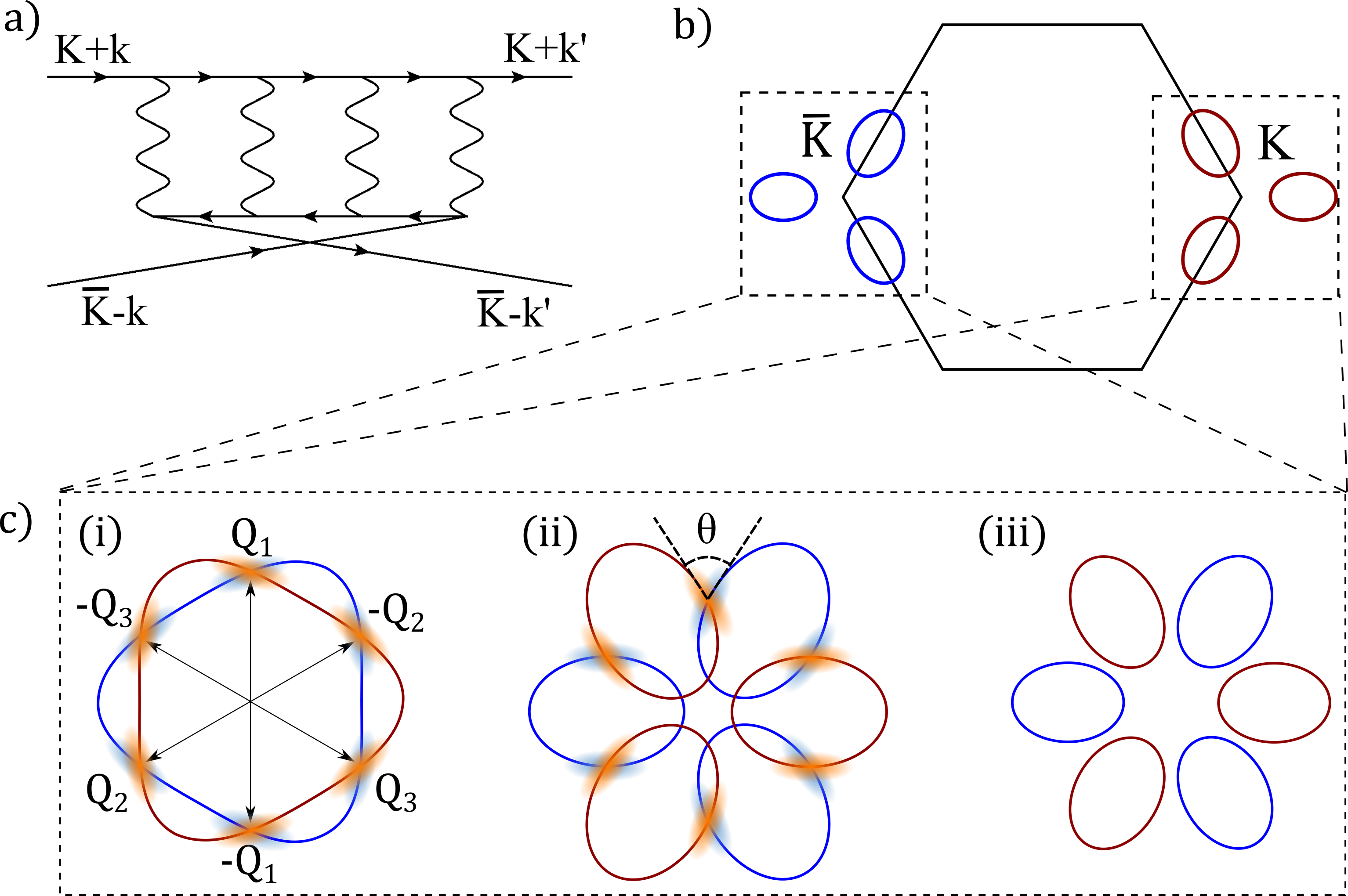
Figure 1: a) A diagrammatic representation of the pairing interaction mediated by isospin mode, a soft mode associated with the intervalley phase coherence (IVC). Identifying valleys ${\boldsymbol{K}}$ and $\bar{{\boldsymbol{K}}}$ with spin up and down maps this interaction to the paramagnon pairing mechanism mediated by ferromagnetic spin fluctuations[7, 8, 9, 10]. At an isospin quantum criticality, this interaction peaks at $\omega+\omega^{\prime}=0$ and ${\boldsymbol{k}}+{\boldsymbol{k}}^{\prime}=0$ (see (1)), resulting in a backscattering-type Cooper pair dynamics. b) Fermi sea pockets located near valleys ${\boldsymbol{K}}$ and $\bar{{\boldsymbol{K}}}$ in BBG bandstructure, which host fermions forming ${\boldsymbol{K}}$-$\bar{{\boldsymbol{K}}}$ Cooper pairs. c) Because of backscattering, pairing develops near “ghost” crossings of Fermi surfaces $\pm Q_{i}$ ($i=1,2,3$) found by superimposing the pockets in valleys ${\boldsymbol{K}}$ (red contours) and $\bar{{\boldsymbol{K}}}$ (blue contours) by a ${\boldsymbol{K}}\to\bar{{\boldsymbol{K}}}$ translation. A single Fermi sea gives non-removable crossings (i), whereas multi-pocket Fermi seas give removable crossings (ii)-(iii), where $\theta$ denotes the angle at the crossing. Transitions between the intersecting and nonintersecting Fermi surfaces (ii) and (iii) induced by tuning the bandstructure terminate the superconducting phases.

Here, through a detailed quantitative comparison to experimental data obtained by tuning SC in several graphene systems, we demonstrate the occurrence of the collinear backscattering kinematics. Specifically, we find direct evidence linking the onset of superconductivity and the abrupt appearance of “ghost valley crossings” between Fermi surfaces in different valleys. This is distinct from conventional ways to stimulate superconductivity by tuning the Fermi level through van Hove points. Identification of an abrupt onset of SC with such crossings limits the possible soft modes that can serve as pairing glue, excluding many of the previously considered scenarios and pinpointing SC driven by the isospin inter-valley-coherent (IVC) mode pictured in Fig.1 and discussed below as the most likely mechanism. Further evidence for this scenario is provided by a significant enhancement of superconducting $T_{\rm c}$ and a characteristic nonmonotonic behavior at SC onset near ghost valley crossing (see (3) and accompanying discussion), which is in good agreement with experimental observations (see Fig.3).

A salient feature of graphene superconductivity that will be important for our analysis is that the two electrons forming a Cooper pair are located in valleys $K$ and $\bar{K}$ which are related by time reversal symmetry. Accordingly, Cooper pair kinematics involves valley-conserving scattering of pair states $({{\boldsymbol{K}}}+{{\boldsymbol{k}}},\bar{{\boldsymbol{K}}}-{{\boldsymbol{k}}})\to({{\boldsymbol{K}}}+{\boldsymbol{k}}^{\prime},\bar{{\boldsymbol{K}}}-{\boldsymbol{k}}^{\prime})$ with ${\boldsymbol{k}},{\boldsymbol{k}}^{\prime}\ll K$. Because of this property, the only type of pairing mechanism that can generate collinear backscattering kinematics with ${\boldsymbol{k}}^{\prime}\approx-{\boldsymbol{k}}$ is the pairing mediated by isospin fluctuations that are softened and activated at quantum criticality [18, 17, 14, 16, 19]. Here, isospin refers to spin and valley. This isospin mode arises from the fluctuations of valley order $\langle\psi_{{\boldsymbol{K}}}^{\dagger}\psi_{\bar{{\boldsymbol{K}}}}\rangle$, the quantity describing the inter-valley coherence (IVC)[38]. To clarify the backscattering nature of the IVC pairing mechanism, we write down the pairing interaction shown diagrammatically in Fig.1. This is directly analogous to the paramagnon pairing mechanism near a ferromagnetic quantum critical point [7, 8, 9, 10]. Standard analysis [see [17, 14, 18] and [39], Sec.B] yields

$$\Gamma_{\omega{\boldsymbol{k}},\omega^{\prime}{\boldsymbol{k}}^{\prime}}=\frac{U}{\kappa|\omega+\omega^{\prime}|+l_{0}^{2}({\boldsymbol{k}}+{\boldsymbol{k}}^{\prime})^{2}+\delta^{2}},$$ (1)

where $U$, $\kappa$, $l_{0}$ are model-specific parameters and $\delta$ denotes the distance to the QCP [39]. Crucially, the two electrons in a Cooper pair are predominantly scattered from the initial momenta of $({\boldsymbol{K}}+{\boldsymbol{k}},\bar{{\boldsymbol{K}}}-{\boldsymbol{k}})$ to the final momenta of $({\boldsymbol{K}}+{\boldsymbol{k}}^{\prime},\bar{{\boldsymbol{K}}}-{\boldsymbol{k}}^{\prime})$ where ${\boldsymbol{k}}^{\prime}\approx-{\boldsymbol{k}}$, namely, backscattering dominates. Indeed, the soft mode describing the IVC instability, which mediates pairing, is the particle-hole ladder shown in Fig.1 for which the momentum transfer is $({\boldsymbol{K}}+{\boldsymbol{k}})-(\bar{{\boldsymbol{K}}}-{\boldsymbol{k}}^{\prime})$. Expanding about the ordering vector $2{\boldsymbol{K}}$ yields a singularity at small $({\boldsymbol{k}}+{\boldsymbol{k}}^{\prime})^{2}$ in (1). This behavior is distinct from the QCP scenarios where pairing mainly benefits from forward-scattering processes, wherein electrons are scattered by a small angle on the Fermi surface, as, e.g., the pairing mediated by nematic fluctuations in iron-based superconductors[40, 41, 42] or pairing through interaction renormalized by valley-polarization fluctuations in graphene bilayer[15]. In these cases the pairing interaction can be modeled by an expression similar to that in (1) with frequencies and momenta entering as $\omega-\omega^{\prime}$ and ${\boldsymbol{k}}-{\boldsymbol{k}}^{\prime}$. In this case the interaction peaks at ${\boldsymbol{k}}^{\prime}\approx{\boldsymbol{k}}$ and $\omega^{\prime}\approx\omega$. Therefore, establishing the backscattering pair kinematics strongly supports the IVC pairing mechanism. Since the Fermi surface ghost crossing signature arises generally in the presence of multiple Fermi pockets and tunable bands, this method can be tested in many superconducting systems such as those found in transition metal dichalcogenides and graphene multilayers[43, 3, 4, 44, 45, 46, 5].

Parenthetically, other scenarios may be considered, such as pairing mediated by antiferromagnetic (AFM) fluctuations, where electrons are predominantly scattered between different parts of the Fermi surface by a large AFM ordering momentum. This mechanism is actively studied in iron pnictides[12, 13], yet it does not appear relevant for graphene.

Figure 2: a) Phase diagram of BBG measured at a finite in-plane magnetic field $B_{\parallel}=0.165$T, adapted from Ref.[4]. The SC phase occurs along the phase boundary between the partially isospin-polarized phase (PIP₂) and an isospin-unpolarized phase (Sym₁₂). b) A zoom-in of the region near SC onset in a). Red and black curves mark the phase boundaries. The solid yellow line, obtained from the free-particle bands in phase Sym₁₂, marks the transition at which the “ghost” ${\boldsymbol{K}}-\bar{{\boldsymbol{K}}}$ Fermi surface crossings abruptly disappear (see insets in the top row). The dashed yellow line, drawn in the region where the free-particle description does not apply, is a guide to the eye. The measured emergence point of SC coincides with the appearance of the Fermi-surface crossings. The inset on the left, adapted from Ref.[4], shows the Fermi surfaces for four isospins in PIP₂ phase.

We will demonstrate the fundamental idea using the setting of Bernal bilayer graphene (BBG) biased by a transverse electric field, a strongly interacting system with a tunable band hosting a superconducting phase[4]. A key experimental finding that points to QCP physics is that the SC phase is a sliver that tracks the phase boundary between a partially-isospin-polarized phase and an unpolarized phase, labeled PIP₂ and Sym₁₂ in Fig.2 following Ref.[4]. The two QCP scenario types introduced above, involving forward scattering and backscattering, are both viable candidates for this system. The former involves valley-polarization order due to Stoner valley imbalance instability in BBG[15], whereas the latter involves IVC order. The IVC scenario has been considered in RTG [17] and it is straightforward to generalize to BBG as will be shown below. Experiments also indicate a peculiar $B$ dependence of SC which persists in a high in-plane magnetic field $B_{\parallel}$ and is activated only above a threshold $B_{\parallel}$. Yet these observations cannot directly distinguish the two QCP scenarios.

However, there is one observation that so far has escaped attention: The SC sliver only exists on a segment of the PIP₂-Sym₁₂ phase boundary – it emerges abruptly upon increasing carrier density along this boundary. The same behavior is found recently in the SC₁ phase of BBG/WSe₂ but not in RTG. As we shall show, this behavior favors a pairing mechanism that involves backscattering, as opposed to the Stoner instability type proposed earlier which involves forward scattering[15].

Next, we consider the backscattering mechanism for superconductivity and its relation to ghost crossings. As we will see, the pairing gap predominantly opens near the crossings of Fermi surfaces in valleys ${\boldsymbol{K}}$ and $\bar{{\boldsymbol{K}}}$ superimposed by a ${\boldsymbol{K}}\to\bar{{\boldsymbol{K}}}$ translation. These points, below referred to as “ghost” crossings, are illustrated in Fig.1 c), where they are labeled $\pm Q_{i}$ ($i=1,2,3$). This result directly follows from the back-scattering nature of the pairing interaction (1), which requires that both momenta ${\boldsymbol{k}}$ and $-{\boldsymbol{k}}$ are found near the Fermi surface in the same valley.

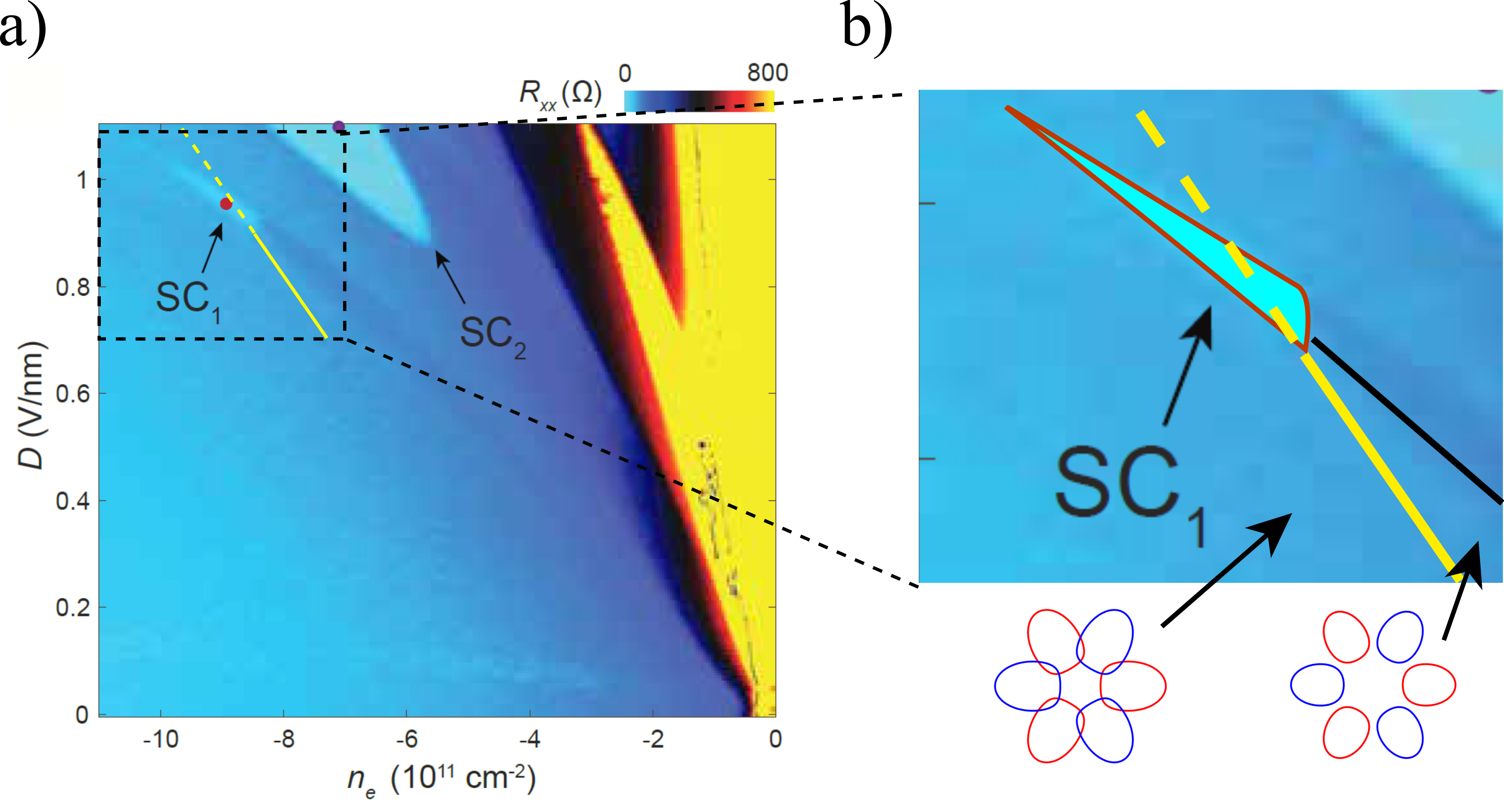
Figure 3: a) Phase diagram of WSe₂-supported BBG, adapted from Ref.[47]. Here, distinct from BBG, the part below the red and black phase boundaries is the “vanilla” phase where no symmetry is broken. The phase above the black phase boundary and SC phase is an ordered phase conjectured in Ref.[47] to be a nematic phase. b) The agreement between theoretically predicted onset of ${\boldsymbol{K}}$-$\bar{{\boldsymbol{K}}}$ Fermi surface crossings (solid yellow line) and the measured superconductivity emergence point for WSe₂-supported BBG. The dashed yellow line, as in Fig.2, is a guide to the eye. The insets in b) illustrate the overlapping and non-overlapping Fermi surfaces. The red and blue curves represent Fermi surfaces in minority isospin species ${\boldsymbol{K}}\downarrow$ and $\bar{{\boldsymbol{K}}}\uparrow$, respectively.

Crucially, these crossings can be switched on and off by varying transverse electric field, an experimental knob tuning the BBG band structure. We anticipate that this change in the bandstructure, illustrated schematically in Fig.1 c) (ii) and c) (iii), leads to an abrupt emergence of SC phase, a notable feature observed in BBG (see Fig.2) and WSe₂-supported BBG[47] (see Fig.3). This leads to a conjecture that the superconductivity in both systems is dominated by a backscattering pairing mechanism. Below we present microscopic analysis for IVC QCP that allows us to verify this conjecture quantitatively by a direct band structure calculation. Though for the WSe₂-supported BBG the IVC phase is not believed to be stabilized[47, 48, 49], we assume that it may be a competing phase so that IVC fluctuations co-exist with nematic fluctuations, with the IVC pairing channel enhanced by nesting at the “ghost” Fermi surface crossing (see below). Our approach reproduces the measured SC emergence points with high accuracy providing strong evidence for pair backscattering. Further, since this behavior cannot be explained by other existing scenarios, such as [15, 50, 51, 52, 53, 54, 55], the IVC pairing scenario stands out as the most probable occurrence in a realistic system.

It is also interesting to mention that in the rhombohedral trilayer graphene where the Fermi sea is an annulus with both its inner and outer Fermi surfaces looking like the one in Fig.1 c) (i)[43, 3]. In this case the ghost crossings remain robust under variation of the electric field and, therefore, we do not expect abrupt emergence or termination of SC phase similar to that seen in BBG. This conclusion is in agreement with the observed phase diagrams [3].

Next, we present the essential points of the microscopic analysis. Due to the observation that pairing gap predominantly opens at $\pm Q_{i}$’s shown in Fig.1, it is convenient to describe pairing in terms of the electron dispersion within the patches around $\pm Q_{i}$’s, treating $\pm Q_{i}$ as a patch index. Namely, we define a gap function near $\pm Q_{i}$ as $\Delta_{{\boldsymbol{K}}\bar{{\boldsymbol{K}}};\pm Q_{i}}({\boldsymbol{k}})$, where ${\boldsymbol{k}}$ is measured from $Q_{i}$, and $k^{\prime}$ is measured from $-Q_{i}$. Here, ${\boldsymbol{k}},{\boldsymbol{k}}^{\prime}\ll k_{F}$. Accordingly, we model the electron energy near $\pm Q_{i}$ as:

$$\epsilon_{\pm i,{\boldsymbol{k}}}=v_{F}{\boldsymbol{n}}_{\pm i}\cdot{\boldsymbol{k}}+|{\boldsymbol{n}}_{\pm i}\times{\boldsymbol{k}}|^{2}/2m_{\perp}$$ (2)

where ${\boldsymbol{n}}_{\pm i}$ are the unit vectors normal to the Fermi surface at $\pm Q_{i}$. Applying this model to describe pairing and keeping only the scattering processes in which an electron is scattered from a patch near $Q_{i}$ to a patch near $-Q_{i}$, which is the most singular contribution, we find

$$\Delta_{{\boldsymbol{K}}\bar{{\boldsymbol{K}}};Q_{i}}({\boldsymbol{k}},\omega)=-\sum_{{\boldsymbol{k}}^{\prime}\omega^{\prime}}\frac{\Gamma_{\omega+\omega^{\prime},{\boldsymbol{k}}+{\boldsymbol{k}}^{\prime}}\Delta_{{\boldsymbol{K}}\bar{{\boldsymbol{K}}};-Q_{i}}({\boldsymbol{k}}^{\prime},\omega^{\prime})}{\omega^{\prime 2}+\epsilon^{2}_{-i,{\boldsymbol{k}}^{\prime}}},$$

The analysis of this equation is detailed in [39]. Below we describe the main predictions.

Since $\Gamma_{\omega+\omega^{\prime},{\boldsymbol{k}}+{\boldsymbol{k}}^{\prime}}$ is positive, the gap equation predicts a sign-changing solution $\Delta_{{\boldsymbol{K}}\bar{{\boldsymbol{K}}};Q_{i}}=-\Delta_{{\boldsymbol{K}}\bar{{\boldsymbol{K}}};-Q_{i}}$(see Sec.D in Ref.[39]). This yields two degenerate pairing channels that respect the symmetry group (see Sec.C in Ref.[39]). These are the p-wave $p_{x}\pm ip_{y}$ channels identical to the ones identified for RTG [17] and moiré graphene [19]. A linear superposition of these two channels gives rise to a $p$-wave channel which breaks the rotational symmetry, which has a $T_{\rm c}$ degenerate with that of $p_{x}\pm ip_{y}$ channels. In a recent experiment[47] in WSe₂-supported BBG samples the SC phases are found to emerge on top of, or next to, a nematic phase where three-fold rotation symmetry is spontaneously broken. This suggests that the $p$-wave superconductivity wins in these systems.

An interesting behavior of SC that is unique to the three-pocket Fermi sea is an increase in $T_{\rm c}$ near the termination of SC phase. Indeed, upon the appearance of ghost crossings the Fermi pockets in two valleys become nearly tangential at the crossing point. In this case, an approximate nesting at the ${{\boldsymbol{K}}}$-$\bar{{\boldsymbol{K}}}$ pocket crossings by a vector $2{\boldsymbol{K}}$ allows pairing to occur on a larger Fermi surface segment near the crossing points, which leads to an enhancement in superconducting $T_{\rm c}$. This behavior is manifest in the expression for $T_{\rm c}$ derived in [39], Sec.E:

$$T_{\rm c}=2\omega_{0}e^{-\frac{1}{\lambda}},\quad\lambda=\frac{U}{8v_{F}l_{0}\delta\sin(\theta/2)},\quad\omega_{0}=\frac{\delta v_{F}}{l_{0}}.$$ (3)

with $\theta$ the angle between the ${{\boldsymbol{K}}}$ and $\bar{{\boldsymbol{K}}}$ Fermi surfaces at the crossing points (see Fig.1 c)). The increase in $T_{\rm c}$ occurs because $\theta$ vanishes when the Fermi surfaces become tangential. We expect the divergence of $\lambda$ at $\theta\to 0$ to be cut off by the dispersion curvature described by the quantity $m_{\perp}$ in (2)); this effect is not manifest in (3) as it is subleading for finite $\theta$. However, $m_{\perp}$ will limit the phase volume in ${\boldsymbol{k}}$-space where pairing can occur when $\theta\rightarrow 0$, thereby, cutting off the divergence of $\lambda$ and $T_{\rm c}$. The enhancement in $T_{\rm c}$ near the termination point probably explains why IVC fluctuations dominate the pairing despite possible presence of other fluctuations, e.g. due to nematic order conjectured in Ref.[47].

Unfortunately, the existing data are insufficient to map out this interesting behavior, though it is somewhat consistent with the superconducting phase in Fig.3 widening near the termination point. Verifying the predicted nonmonotonic behavior in $T_{\rm c}$ near the termination point is an interesting direction for future experiments.

Next, we use a realistic bandstructure to obtain a condition for the ghost Fermi surface crossings to exist and demonstrate an agreement with the observed onset of superconductivity. We first present the analysis for WSe₂-supported BBG. In Ref.[47] two superconductivity phases were found. Here, we focus on the SC₁ phase, which emerges from an isospin-unpolarized parent state. The phase SC₂ emerges from a parent state with a pocket polarization[47] that needs an analysis that accounts for the interaction effects, which we leave to future work.

We predict the onset of valley-crossings by numerically calculating the single-particle band dispersion in the isospin-unpolarized phase. We model the single-particle in WSe₂-supported BBG using the Hamiltonian

$$H=H_{\rm BBG}+H_{\rm SOI}.$$ (4)

The first term $H_{\rm{BBG}}$ is the four-band tight-binding model given in the basis $\left\{c_{A,1}^{\eta,s},c_{B,1}^{\eta,s},c_{A,2}^{\eta,s},c_{B,2}^{\eta,s}\right\}$ (with A and B the sublattice indices, 1 and 2 the layer indices, $\eta=\pm 1$ a valley label and $s$ the spin index) [56, 57] and [39] Sec.A:

$$H_{\rm{\rm BBG}}=\left(\begin{matrix}u/2&v\pi^{\dagger}&-v_{4}\pi^{\dagger}&v_{3}\pi\\ v\pi&u/2+\Delta^{\prime}&t_{1}&-v_{4}\pi^{\dagger}\\ -v_{4}\pi&t_{1}&-u/2+\Delta^{\prime}&v\pi^{\dagger}\\ v_{3}\pi^{\dagger}&-v_{4}\pi&v\pi&-u/2\end{matrix}\right)$$ (5)

where $\pi=\hbar\left(\eta k_{x}+ik_{y}\right)$, $k_{x}$ and $k_{y}$ are the $x$ and $y$ components of momentum measured from ${{\boldsymbol{K}}}$ or $\bar{{\boldsymbol{K}}}$. The quantity $u$ is the interlayer bias, $t_{1}$ is the interlayer hopping parameter, $v$, $v_{3}$, $v_{4}$ are associated with microscopic hopping amplitudes of the values given in [57]. The second term $H_{\rm{SOI}}$, (4), represents an Ising spin-orbital interaction (SOI) induced by the proximate WSe₂ layer, which takes the valley Ising form[46]:

$$H_{\rm{\rm SOI}}=\lambda_{\rm I}\eta\sigma_{z}$$ (6)

where $\eta=\pm 1$ for valley ${{\boldsymbol{K}}}$ and $\bar{{\boldsymbol{K}}}$, $\sigma_{z}$ is the Pauli matrix for spin in the out-of-plane direction.

To determine how the onset of Fermi surface crossings compares with measured SC phases, two parameters in model (4) must be obtained by careful analysis of existing data. One is the interlayer bias $u$, which is proportional to the transverse electric field $D$, yet the ratio between $u$ and $D$ in general is not exactly known (see discussion below). Another is the spin-orbit coupling $\lambda_{\rm I}$.

We determine these two quantities using the quantum oscillations measured in Ref.[47]. This measurement accurately gives the carrier densities where two distinct transitions of Fermi surface topology occur in the minority isospin species ${{\boldsymbol{K}}}\downarrow$ and $\bar{{\boldsymbol{K}}}\uparrow$. One is the transition from a single Fermi sea to an annular Fermi sea occurs at $n=9.9\times 10^{11}\rm{cm}^{-2}$. The other is the transition from the annular Fermi sea to a three-pocket Fermi sea occurs at $n=9.7\times 10^{11}\rm{cm}^{-2}$. Using these two data points as constraints, we are able to determine the numerical values of the two unknown parameters:

$$\frac{u}{\rm{meV}}=\frac{(0.047\pm 0.001)eD}{\rm{mV/nm}},\quad\lambda_{\rm I}=(7\pm 1)\rm{meV}.$$

Using these values, we study the evolution of Fermi seas within the symmetry-unbroken “vanilla” phase. We focus on the Fermi seas of the minority isospin species as the majority isospin species feature a single Fermi sea that does not experience any qualitative change in this regime. In the regime where SC₁ phase occurs, the majority species feature valley crossings of the ${\boldsymbol{K}}$ and $\bar{{\boldsymbol{K}}}$ Fermi seas with an order-one angle $\theta\sim O(1)$ at the crossing and, consequently, no enhancement in superconductivity due to small $\theta$ values similar to the one demonstrated by the minority species. We therefore focus on minority species, deferring the analysis of majority species till later. We determine the transition from overlapping to non-overlapping Fermi seas in minority species, finding a transition marked by the yellow lines in Fig.3. The solid yellow line lies inside the symmetry-unbroken “vanilla” phase where a single-particle band calculation can be trusted. The dashed yellow line drawn across the ordered phase where a single-particle band calculation is invalid merely provides a guide to the eye. Notably, the yellow line crossing with the phase boundary agrees well with the SC phase onset. This provides strong evidence for the pairing governed by a back-scattering mechanism, such as the IVC QCP scenario.

We note that the value of $\lambda_{\rm I}$ extracted and used above is a few times greater than the value $\lambda^{(0)}_{\rm I}=1.6$ meV inferred from measurements in a strong out-of-plane $B$ field [47]. We believe that this discrepancy is reasonable. Indeed, the value of $\lambda_{\rm I}$ that should be plugged in our simulation is not the bare SOI strength, but rather the effective interaction renormalized by strong interactions in a flat-bottom BBG band. The vertex corrections that govern this renormalization are expected to be large since the system is in the regime close to all kinds of spin and valley Stoner instabilities. In contrast, $\lambda^{(0)}_{I}$ measured in a large $B$ field[47] is largely insensitive to this physics, which explains the above disparity in $\lambda_{I}$ values.

Next, we turn to the BBG/hBN case[4]. We continue to use the four-band model given in (5). Here, however, unlike the case of WSe₂-supported BBG, the relation between the interlayer bias parameter $u$ and the experimental displacement field $D$ is not accurately known. For BBG/hBN quantum oscillation measurements[4] do not provide sufficient information to extract the ratio between interlayer bias $u$ and displacement field $D$. However they do give useful upper and lower bounds for $u/D$.

Namely, quantum oscillation measurements [4] reveal that: 1) the isospin-unpolarized Sym₄ phase below the isospin-polarized PIP₂ phase (shown in Fig. 2 b) has a single Fermi surface per isospin; 2) the isospin-unpolarized Sym₁₂ phase above PIP₂ features three distinct pockets per isospin. We find that in order to reproduce these two observations, the value $u/D$ should fall in the range: $0.057<\frac{u}{eD\cdot\rm{nm}}<0.072$. Accordingly, as a best guess, we pick a value in the middle of this window, $\frac{u}{eD\cdot\rm{nm}}=0.065$. With this value, we derive the transition line between overlapping and non-overlapping Fermi seas, indicated as the yellow line in Fig.2, which closely matches the emergence point of the SC phase.

It is worth noting that several experiments have attempted to measure the $u/D$ ratio for BBG, yielding vastly different values that do not fall within the range inferred from our fermiology analysis. Namely, Refs.[58] and [5] find $\frac{u}{eD\cdot\rm{nm}}=0.1$ and $0.033$, respectively. Due to significant variations in values, likely due to electrostatic differences in devices, we refrained from using them directly. Instead, we selected $u/D$ as described above to predict fermiology that best matches the measurements.

To restate the main result of our analysis, in both BBG and in BBG/WSe₂ the lines that mark the emergence of ghost Fermi surface crossings match perfectly the points of the onset of superconductivity. As discussed above, the emergence of valley crossings strongly impacts the pair scattering kinematics, favoring backscattering. To the contrary, it has little impact on the density of states at the Fermi level or the e-e interaction strength. Therefore the observed behavior is difficult to understand within a conventional BCS superconductivity framework but is naturally explained by the IVC superconductivity mechanism.

This conclusion is further supported by the nonmonotonic behavior of superconductivity near the onset (a rise followed by a drop) observed in BBG/WSe₂. This observation is explained by the enhancement of pairing at small angles $\theta$ between Fermi surfaces at the ghost crossing discussed above. It is interesting to compare the nonmonotonic behavior of superconductivity in BBG/WSe₂ with the monotonic behavior observed at superconductivity onset in BBG/hBN samples. We believe that this difference can be attributed to the constraints imposed by isospin orders and Fermiology. Specifically, the SC phase in BBG/hBN must lie outside the PIP₂ phase which is not necessarily compatible with the SC order, and below the boundary where valley crossings occur (yellow line in Fig. 2). These constraints limit the SC phase to a narrow wedge in the phase diagram (Fig. 2), preventing the enhancement of the SC phase at the onset of valley crossings. In comparison, in the BBG/WSe₂ these constraints are lifted. Since the “vanilla” phase lies below the phase boundary, the onset of valley crossings (solid yellow line in Fig. 3) extends downwards and therefore does not constrain the SC phase.

Lastly, we believe that the IVC pairing revealed by our analysis is generally applicable to other observed SC phases, such as the SC₂ phase in BBG/WSe₂. Here a conclusive analysis would require more knowledge of the isospin phase diagram, which is currently being investigated by several groups [48, 49]. Nonetheless, the SC₂ phase, which is a wedge embedded between different isospin orders, shows an abrupt onset which is likely related to a ghost valley crossing (see Fig. 3).

In conclusion, the sudden appearance of SC phases coincides with the appearance of the ${{\boldsymbol{K}}}$-$\bar{{\boldsymbol{K}}}$ ghost Fermi surface crossings in both BBG and WSe₂-supported BBG. This behavior suggests that quantum-critical fluctuations drive the pairing in both systems, favoring a backscattering-type pairing interaction due to the IVC order as the glue for superconductivity over other candidates like valley-polarization order [15]. Overall, it is not compatible with conventional phonon mechanisms[50, 51], nor with the conventional Kohn-Luttinger mechanisms[53, 54], pointing to a mechanism that involves a soft quantum-critical mode as a pairing glue. Last but not least, it highlights tuning bands through ghost crossings as an attractive pathway to enhance superconductivity.

We thank A. F. Young and S. Nadj-Perge for sharing unpublished data, and A. V. Chubukov and J. G. Analytis for fruitful discussions. This work was supported by the Science and Technology Center for Integrated Quantum Materials, National Science Foundation Grant No. DMR1231319, and Army Research Office Grant No. W911NF-18-1-0116. P. L. acknowledges the support by DOE office of Basic Sciences Grant No. DE-FG02-03ER46076.

Appendix A Model

In this section we provide details on the model used in the main text. Our single-particle Hamiltonian is identical to that in Ref.[56] whereas the interaction model is same as that in Ref.[15].

The electron single-particle Hamiltonian for BBG is a $4\times 4$ matrix expressed in the basis of $\left\{c_{A,1}^{\eta,s},c_{B,1}^{\eta,s},c_{A,2}^{\eta,s},c_{B,2}^{\eta,s}\right\}$ (A and B are sublattice indices, 1 and 2 are the layer indices, $\eta=\pm 1$ labels valley ${{\boldsymbol{K}}}$ and $\bar{{\boldsymbol{K}}}$, and $s$ is the spin index) [56]:

$$H_{\rm BBG}=\left(\begin{matrix}u/2&v\pi^{\dagger}&-v_{4}\pi^{\dagger}&v_{3}\pi\\ v\pi&u/2+\Delta^{\prime}&t_{1}&-v_{4}\pi^{\dagger}\\ -v_{4}\pi&t_{1}&-u/2+\Delta^{\prime}&v\pi^{\dagger}\\ v_{3}\pi^{\dagger}&-v_{4}\pi&v\pi&-u/2\end{matrix}\right)$$ (7)

where $\pi=\hbar\left(\eta k_{x}+ik_{y}\right)$, $k_{x}$ and $k_{y}$ are the $x$ and $y$ components of momentum measured from ${{\boldsymbol{K}}}$ or $\bar{{\boldsymbol{K}}}$. This Hamiltonian gives a trigonally-warped conduction band. In the isospin-polarized phase on which the SC emerges, quantum oscillations measurement shows that the Fermi sea in each isospin consists of three pockets, as shown in panels (ii) and (iii) of Fig.1 c) in main text.

The electron-electron interaction in BBG is modeled as an intervalley local interaction

$$H_{int}^{(0)}=\frac{1}{2}U\sum_{l,\alpha,q,\tau,s}:\rho^{(0)}_{q,\alpha,l,\tau,s}\rho^{(0)}_{-q,\alpha^{\prime},l^{\prime},\tau^{\prime},s^{\prime}}:$$ (8)

where $\rho^{(0)}_{q,\alpha,l,\eta,s}=\sum_{{\boldsymbol{k}}}c^{\dagger}_{{\boldsymbol{k}}+{\boldsymbol{q}},\alpha,l,\eta,s}c_{{\boldsymbol{k}},\alpha,l,\eta^{\prime},s^{\prime}}$. In the analysis below we project $H_{int}^{(0)}$ onto the conduction band which is the only band relevant for SC. In the regime of $D$ much larger than all other elements in Eq.(7), the projected interaction Hamiltonian is approximately given by

$$H_{int}=\frac{1}{2}U\sum_{q,\tau\tau^{\prime}ss^{\prime}}:\rho_{q,\eta,s}\rho_{-q,\eta^{\prime},s^{\prime}}:,\quad$$ (9)

Here the quantities $\rho_{q,\eta,s}$ are projected density operators defined as $\rho_{q,\tau,s}=\sum_{{\boldsymbol{k}}}\psi^{\dagger}_{{\boldsymbol{k}}+{\boldsymbol{q}},\tau,s}\psi_{{\boldsymbol{k}},\tau,s}$, where $\psi_{{\boldsymbol{k}},\tau,s}$ is an electron operator projected onto the conduction band.

Appendix B The scattering vertex function near IVC instability

In this section, we consider the Cooper pair scattering vertex function mediated by the soft mode describing IVC order fluctuations in the normal state. This quantity is overall similar to that considered in Ref.[17, 19]. However, unlike in Ref.[19] which directly starts from a spin-valley-fermion model, here we derive it from microscopic model Eq.(5) and Eq.(9) explicitly. Our derivation below does not account for the intervalley exchange interaction considered in Ref.[17]. As we will see, the frequency dependence of the Cooper pair scattering vertex function slightly differs from that considered in Ref.[19, 17].

We start by defining the IVC order parameter as follows[59]

$$O_{\rm IVC}=\sum_{s,{\boldsymbol{k}}}\langle\psi^{\dagger}_{{\boldsymbol{k}},\eta,s}\tau_{x,\eta\eta^{\prime}}\psi_{{\boldsymbol{k}},\eta^{\prime},s}\rangle$$ (10)

here $\tau_{x}$ is the Pauli matrix in $x$ direction. Near the onset of this order, the most divergent contribution to vertex function is dominated by the ladder diagram shown in main text Fig.1 a), in which a Cooper pair at momenta ${{\boldsymbol{K}}}+{\boldsymbol{k}}$ and $\bar{{\boldsymbol{K}}}-{\boldsymbol{k}}$ is scattered to a pair at ${{\boldsymbol{K}}}+{\boldsymbol{k}}^{\prime}$ and $\bar{{\boldsymbol{K}}}-{\boldsymbol{k}}^{\prime}$. The scattering vertex given by this diagram is clearly a function of the total frequency $\omega+\omega^{\prime}$ and the total momentum ${\boldsymbol{k}}+{\boldsymbol{k}}^{\prime}$ and takes the following form:

$$\Gamma_{\omega+\omega^{\prime},{\boldsymbol{k}}+{\boldsymbol{k}}^{\prime}}=\frac{U}{1+U\Pi_{{{\boldsymbol{K}}}\bar{{\boldsymbol{K}}}}(\omega+\omega^{\prime},{\boldsymbol{k}}+{\boldsymbol{k}}^{\prime})},$$ (11)

$$\Pi_{{{\boldsymbol{K}}}\bar{{\boldsymbol{K}}}}(\nu,{\boldsymbol{q}})=\sum_{\omega,{\boldsymbol{p}}}G_{K}(\omega+\nu,{\boldsymbol{k}}+{\boldsymbol{q}})G_{\bar{{\boldsymbol{K}}}}(\omega,{\boldsymbol{k}})$$ (12)

This interaction diverges for $\omega+\omega^{\prime}=0,{\boldsymbol{k}}+{\boldsymbol{k}}^{\prime}=0$ because the Stoner criterion in IVC channel is given by[16]

$$1+U\Pi_{{{\boldsymbol{K}}}\bar{{\boldsymbol{K}}}}(0,0)\rightarrow 0$$ (13)

Distinct from the valley-polarization susceptibility which contains a frequency-dependent term singular in momentum $\frac{|\nu|}{|q|}$ due to Landau damping, the intervalley particle-hole susceptibility does not contain such a term. This is because the inter-valley zero-frequency momentum-${{\boldsymbol{K}}}-{\bar{{\boldsymbol{K}}}}$ particle-hole excitations have a measure-zero phase space. Namely, in our case, the $q=0$ inter-valley particle-hole gap closes only at six points: ${\boldsymbol{k}}=\pm{\boldsymbol{Q}}_{i}$, ($i=1,2,3$). This is distinct from usual particle-hole excitations in Fermi liquid where the $q=0$ particle-hole excitation is gapless for any ${\boldsymbol{k}}$ on the Fermi surface.

To see this explicitly, we calculate the frequency and momentum dependence inter-valley particle-hole susceptibility below and find

$$\Pi_{{{\boldsymbol{K}}}\bar{{\boldsymbol{K}}}}(i\nu,q)=\Pi_{{{\boldsymbol{K}}}\bar{{\boldsymbol{K}}}}(0,0)+\frac{3|\nu|}{4\pi v_{F}^{2}\sin\theta}+\alpha q^{2}.$$ (14)

Here $\alpha$ is a parameter depending on band dispersion details. $\theta$ is the angle between the fermi surface in valley ${{\boldsymbol{K}}}$ and that in valley $\bar{{\boldsymbol{K}}}$ at the valley-crossing points. In the analysis below, we take $\sin\theta\sim O(1)$ unless specified otherwise.

To see this explicitly, below we pause and derive the frequency and momentum dependence of IVC susceptibility Eq.(14). As we will see, the susceptibility does not contain a Landau damping term $|\nu|/|q|$ in the denominator. This is quite different from the textbook spin-susceptibility (e.g., see Ref.[60]) or the valley-polarization susceptibility discussed in Ref.[15] where Landau damping term shows up.

$$\Pi_{{{\boldsymbol{K}}}\bar{{\boldsymbol{K}}}}(i\nu,q) =\sum_{\omega,p}G_{{\boldsymbol{K}}}(\omega+\nu,{\boldsymbol{k}}+{\boldsymbol{q}})G_{\bar{{\boldsymbol{K}}}}(\omega,{\boldsymbol{k}})$$ (15)

$$=\sum_{{\boldsymbol{k}},\omega}\frac{f_{{\boldsymbol{k}}+}-f_{{\boldsymbol{k}}-}}{\epsilon_{{\boldsymbol{k}}+}-\epsilon_{{\boldsymbol{k}}-}-i\nu},$$ (16)

where ${\boldsymbol{k}}_{\pm}={\boldsymbol{k}}\pm\frac{{\boldsymbol{q}}}{2}\pm{{\boldsymbol{K}}}$. As a reminder, $\bar{{\boldsymbol{K}}}=-{{\boldsymbol{K}}}$.

$$\Pi_{{{\boldsymbol{K}}}\bar{{\boldsymbol{K}}}}(i\nu,0) =\sum_{{\boldsymbol{k}}}\frac{\left(f_{{{\boldsymbol{K}}}+{\boldsymbol{k}}}-f_{\bar{{\boldsymbol{K}}}+{\boldsymbol{k}}}\right)\left(\epsilon_{{{\boldsymbol{K}}}+{\boldsymbol{k}}}-\epsilon_{\bar{{\boldsymbol{K}}}+{\boldsymbol{k}}}+i\nu\right)}{(\epsilon_{{{\boldsymbol{K}}}+{\boldsymbol{k}}}-\epsilon_{\bar{{\boldsymbol{K}}}+k})^{2}+\nu^{2}}$$ (17)

$$=6\sum_{k}\frac{\left(f_{{{\boldsymbol{K}}}+{\boldsymbol{Q}}+{\boldsymbol{k}}}-f_{\bar{{\boldsymbol{K}}}+{\boldsymbol{Q}}+{\boldsymbol{k}}}\right)\left(\Delta{\boldsymbol{v}}\cdot{\boldsymbol{k}}+i\nu\right)}{\left(\Delta{\boldsymbol{v}}\cdot{\boldsymbol{k}}\right)^{2}+\nu^{2}},\quad\Delta{\boldsymbol{v}}={\boldsymbol{v}}_{{{\boldsymbol{K}}}+{\boldsymbol{Q}}}-{\boldsymbol{v}}_{\bar{{\boldsymbol{K}}}+{\boldsymbol{Q}}}$$ (18)

$$=-6\int_{-k_{F}}^{k_{F}}\frac{dk_{x}}{2\pi}\frac{2k_{x}\sin\theta}{2\pi}\frac{2v_{F}k_{x}\sin\theta}{\left(2v_{F}k_{x}\sin\theta\right)^{2}+\nu^{2}}.$$ (19)

Here $\theta$ is the angle between the fermi surface in valley ${{\boldsymbol{K}}}$ and that in valley $\bar{{\boldsymbol{K}}}$ at the valley-crossing points. To evaluate this integral properly, we calculate the difference between the dynamical polarization function $\Pi_{{{\boldsymbol{K}}}\bar{{\boldsymbol{K}}}}(i\nu,0)$ and the static polarization function $\Pi_{{{\boldsymbol{K}}}\bar{{\boldsymbol{K}}}}(0,0)$:

$$\Pi_{{{\boldsymbol{K}}}\bar{{\boldsymbol{K}}}}(i\nu,0)-\Pi_{{{\boldsymbol{K}}}\bar{{\boldsymbol{K}}}}(0,0)=6\int_{-k_{F}}^{k_{F}}\frac{dk_{x}}{(2\pi)^{2}v_{F}}\frac{\nu^{2}}{\left(2v_{F}k_{x}\sin\theta\right)^{2}+\nu^{2}}=\frac{3|\nu|}{4\pi v_{F}^{2}\sin\theta}.$$ (20)

This result is the leading order frequency dependence in $\Pi_{{{\boldsymbol{K}}}\bar{{\boldsymbol{K}}}}(i\nu,0)$.

Next, we determine the form of leading order momentum dependence from symmetry. We know from $C_{3}$ rotation symmetry that the momentum-dependent part of intervalley particle-hole susceptibility $\Pi_{{{\boldsymbol{K}}}\bar{{\boldsymbol{K}}}}(0,{\boldsymbol{q}})$ has to be a function of $q^{2}$. Therefore, for small $q$ ($q\ll k_{F}$),

$$\Pi_{{{\boldsymbol{K}}}\bar{{\boldsymbol{K}}}}(0,{\boldsymbol{q}})=\Pi_{{{\boldsymbol{K}}}\bar{{\boldsymbol{K}}}}(0,0)+\alpha q^{2}.$$ (21)

Here $\alpha$ is a parameter depending on band dispersion details. Then, accounting for both frequency dependence Eq.(20) and momentum dependence Eq.(21), we arrive at the expression of intervalley susceptibility $\Pi_{{{\boldsymbol{K}}}\bar{{\boldsymbol{K}}}}(i\nu,q)$ given in Eq.(14).

With the results of IVC susceptibility Eq.(14) derived above, we proceed to derive the pairing interaction. Plugging Eq.(14) and Eq.(13) into Eq.(11) we find the pairing interaction $\Gamma_{kk^{\prime}}$ that takes the following form given in main text Eq.(1)

$$\Gamma_{\omega{\boldsymbol{k}},\omega^{\prime}{\boldsymbol{k}}^{\prime}}=\frac{U}{\kappa|\omega+\omega^{\prime}|+l_{0}^{2}({\boldsymbol{k}}+{\boldsymbol{k}}^{\prime})^{2}+\delta^{2}},$$ (22)

with the parameter $\kappa=\frac{3U}{4\pi v_{F}^{2}\sin\theta}$ and the lengthscale $\l_{0}$ is defined as $l_{0}=U\alpha$. For simplicity, here we take $l_{0}=1/k_{F}$ since it is the only lengthscale in this problem. The quantity $\delta$ describes the “distance” from the IVC quantum criticality, it is defined as $\delta=\sqrt{1+U\Pi_{{{\boldsymbol{K}}}\bar{{\boldsymbol{K}}}}(0,0)}$. Eq.(13) indicates that $\delta\rightarrow 0$ near the IVC instability.

This scattering amplitude has a positive sign, which is naively pair-breaking. However, unlike the VP-mediated interaction which is divergent at a small angle scattering ${\boldsymbol{k}}^{\prime}={\boldsymbol{k}}$, the strength of this interaction is maximized for backward scattering $k^{\prime}=-k$ since $\delta\rightarrow 0$. This indicates an attractive pairing interaction in the non-s-wave channel.

This scenario resembles the spin-fluctuation-mediated near a ferromagnetic quantum critical point[10, 61], where spin fluctuation generates a repulsive backward scattering, leading to an effective pairing interaction (attraction) in the $p$-wave channel. However, there is some difference in our case, since enhanced backward scattering here is intravalley scattering ${{\boldsymbol{K}}}+{\boldsymbol{p}}\rightarrow{{\boldsymbol{K}}}-{\boldsymbol{p}}$, rather than ${\boldsymbol{p}}\rightarrow-{\boldsymbol{p}}$ in usual metals. Since ${{\boldsymbol{K}}}+{\boldsymbol{p}}$ is not associated with ${{\boldsymbol{K}}}-{\boldsymbol{p}}$ by symmetry operation (see discussion below), they cannot, in general, simultaneously get close to the Fermi surface. This suggests that such ${{\boldsymbol{K}}}+{\boldsymbol{p}}\rightarrow{{\boldsymbol{K}}}-{\boldsymbol{p}}$ scattering does not always contribute to pairing, except for some special momentum $p$. Below, we will discuss this in detail.

Appendix C Symmetry analysis of the superconducting gap function

In this section, we describe the symmetry of the pairing gap function $\Delta_{{\boldsymbol{K}}\bar{{\boldsymbol{K}}}}$. This symmetry analysis, which is essentially the same as that in Ref.[17], is required for the classification of different pairing channels and for identifying the leading pairing channel.

To start, we describe the superconductivity in BBG using the following BCS Hamiltonian:

$$H_{BCS}=\left(\begin{matrix}\epsilon_{{{\boldsymbol{K}}}+{\boldsymbol{k}}}&\Delta_{{{\boldsymbol{K}}}\bar{{\boldsymbol{K}}}}\\ \overline{\Delta}_{{{\boldsymbol{K}}}\bar{{\boldsymbol{K}}}}&-\epsilon_{\bar{{\boldsymbol{K}}}-{\boldsymbol{k}}}\end{matrix}\right)$$ (23)

where $\Delta_{{{\boldsymbol{K}}}\bar{{\boldsymbol{K}}}}$ represents the anomalous pairing vertex. Here we have suppressed the physical spin indices $\uparrow$/$\downarrow$ since we are focusing on the parallel spin pairing, i.e. either $\uparrow\uparrow$ pair or $\downarrow\downarrow$ pair (see main text). This Hamiltonian yields the following linearized self-consistency equation:

$$\Delta_{{{\boldsymbol{K}}}\bar{{\boldsymbol{K}}}}({\boldsymbol{k}},\omega)=-\sum_{{\boldsymbol{k}}^{\prime}\omega^{\prime}}\frac{\Gamma_{\omega+\omega^{\prime},{\boldsymbol{k}}+{\boldsymbol{k}}^{\prime}}\Delta_{{{\boldsymbol{K}}}\bar{{\boldsymbol{K}}}}({\boldsymbol{k}}^{\prime},\omega^{\prime})}{\omega^{\prime 2}+\epsilon^{2}_{{{\boldsymbol{K}}}+{\boldsymbol{k}}^{\prime}}}$$ (24)

where we have accounted for the frequency and momentum dependence of the pairing vertex $\Delta_{{{\boldsymbol{K}}}\bar{{\boldsymbol{K}}}}$ since $\Gamma$ has a strong frequency and momentum dependence. Below we look for the leading pairing channel through symmetry analysis.

To this end, we proceed as follows: we first identify the symmetries in biased Bernal bilayer graphene. Based on that, we can write down all symmetry-allowed pairing channels $\Delta_{{{\boldsymbol{K}}}\bar{{\boldsymbol{K}}}}({\boldsymbol{k}})$. Then identify channels that maximally benefit from the singularity of $\Gamma_{{{\boldsymbol{K}}}\bar{{\boldsymbol{K}}}}$. Finally, we work out the BCS pairing self-consistency equation in these (degenerate) channels and discuss the higher-order effects which select one channel from them.

The biased bilayer graphene has the following symmetries: a rotation $C_{3}$ around an axis perpendicular to the graphene plane, a mirror reflection $\mathcal{M}_{y}$ (a mirror lying in the $yz$-plane) that maps ${{\boldsymbol{K}}}$ to $\bar{{\boldsymbol{K}}}$. In addition, there is the time-reversal symmetry in the absence of the applied $B$ field. In the presence of $B_{\parallel}$ which couples only to spin, there is an orbital time-reversal symmetry left, which is denoted by $\mathcal{T}$. We note parenthetically that the inversion symmetry and the twofold rotation that swaps AB sites are both broken by the transverse field $D$.

To understand the symmetry of $\Delta_{{{\boldsymbol{K}}}\bar{{\boldsymbol{K}}}}$, we need to understand the symmetry of the Hamiltonian in one valley. The $C_{3}$ operator, which maps $\psi_{{{\boldsymbol{K}}}+{\boldsymbol{k}}}\rightarrow\psi_{{{\boldsymbol{K}}}+C_{3}{\boldsymbol{k}}}$ is preserved in each valley whereas the mirror symmetry $\mathcal{M}_{y}$ and time reversal $\mathcal{T}$ are both individually broken in each valley. However, the Hamiltonian is invariant under a combination of these two symmetry operators $\mathcal{M}_{y}\mathcal{T}$. In sum, the symmetry group is given by:

$$G=\left\{1,C_{3},C_{3}^{2},\mathcal{M}_{y}\mathcal{T},C_{3}\mathcal{M}_{y}\mathcal{T}C_{3}^{-1},C_{3}^{-1}\mathcal{M}_{y}\mathcal{T}C_{3}\right\}$$ (25)

Therefore, the gap function $\Delta_{{{\boldsymbol{K}}}\bar{{\boldsymbol{K}}}}({\boldsymbol{k}})$ that respects the symmetry should obtain an overall phase under $C_{3}$ and $\mathcal{M}_{x}\mathcal{T}$, so we can write:

$$\Delta_{{{\boldsymbol{K}}}\bar{{\boldsymbol{K}}}}(C_{3}k)=e^{i\phi_{1}}\Delta_{{{\boldsymbol{K}}}\bar{{\boldsymbol{K}}}}({\boldsymbol{k}}),\quad\phi_{1}=0,\pm\frac{2\pi}{3},$$ (26)

$$\Delta_{{{\boldsymbol{K}}}\bar{{\boldsymbol{K}}}}(\mathcal{M}_{y}\mathcal{T}{\boldsymbol{k}})=e^{i\phi_{2}}\Delta_{{{\boldsymbol{K}}}\bar{{\boldsymbol{K}}}}({\boldsymbol{k}}),\quad\phi_{2}=\pm\pi.$$ (27)

We find that there are six possibilities in total: $\phi_{1}$ can take three values, whereas $\phi_{2}$ can take two values.

Appendix D The leading pairing channel

In this section, we argue that $p$-wave spin-triplet channel is the leading one in BBG based on symmetry classification. A similar result is obtained in Ref.[17] through numerical calculation.

Which pairing channel is the strongest? To answer this question, we need to find the channels that maximally benefit from the singularity of pairing interaction $\Gamma_{{\boldsymbol{k}}{\boldsymbol{k}}^{\prime}}$. Given that the singularity of $\Gamma_{{\boldsymbol{k}}{\boldsymbol{k}}^{\prime}}$ occurs at ${\boldsymbol{k}}=-{\boldsymbol{k}}$, and that the SC gap function $\Delta_{{{\boldsymbol{K}}}\bar{{\boldsymbol{K}}}}({\boldsymbol{k}})$ is nonzero only for ${\boldsymbol{k}}$ near the Fermi surface, the strongest pairing channel is dominated by $\Delta_{{{\boldsymbol{K}}}\bar{{\boldsymbol{K}}}}$ at the momentum ${\boldsymbol{Q}}$ such that ${\boldsymbol{Q}}$ and $-{\boldsymbol{Q}}$ are both on the Fermi surface. To satisfy this, one way is to find a ${\boldsymbol{Q}}$ on the Fermi surface so that it is related to $-{\boldsymbol{Q}}$ through point group symmetry operation. Clearly, $C_{3}$ cannot relate ${\boldsymbol{Q}}$ and $-{\boldsymbol{Q}}$, but $\mathcal{M}_{y}\mathcal{T}$, $C_{3}\mathcal{M}_{y}\mathcal{T}C_{3}^{-1}$ and $C_{3}^{-1}\mathcal{M}_{y}\mathcal{T}C_{3}$ can achieve this goal. As a result, we find six points $\pm Q_{i}$ ($i=1,2,3$) that satisfy this requirement, in which three ${\boldsymbol{Q}}_{i}$’s are related by $C_{3}$ rotation. Alternatively, we can determine such ${\boldsymbol{Q}}$’s geometrically by Fig.1c) in the main text, where ${\boldsymbol{Q}}$’s are given by the six intersections of superimposed Fermi surfaces in valley ${{\boldsymbol{K}}}$ and $\bar{{\boldsymbol{K}}}$.

It is convenient to describe the structure of the pairing function $\Delta_{{{\boldsymbol{K}}}\bar{{\boldsymbol{K}}}}$ using a valley-crossing-point model, where we define a gap function in each valley-crossing points $\pm{\boldsymbol{Q}}_{i}$ as $\Delta_{{{\boldsymbol{K}}}\bar{{\boldsymbol{K}}};\pm{\boldsymbol{Q}}_{i}}({\boldsymbol{k}})$. The electron energy near valley-crossing point ${\boldsymbol{Q}}_{i}$ is modeled as:

$$\epsilon_{\pm i,{\boldsymbol{k}}}=v_{F}{\boldsymbol{n}}_{\pm i}\cdot{\boldsymbol{k}}+\frac{|{\boldsymbol{n}}_{\pm i}\times{\boldsymbol{k}}|^{2}}{2m_{\perp}}$$ (28)

where ${\boldsymbol{n}}_{i}$ is the unit normal vector of Fermi surface at $Q_{i}$. In this model, we define a gap function in each valley-crossing point $\pm{\boldsymbol{Q}}_{i}$ as $\Delta_{{{\boldsymbol{K}}}\bar{{\boldsymbol{K}}};\pm Q_{i}}({\boldsymbol{k}})$. According to the symmetry constraint given in Eq.(26), they satisfy

$$\Delta_{{{\boldsymbol{K}}}\bar{{\boldsymbol{K}}};{\boldsymbol{Q}}_{i}}({\boldsymbol{k}})=e^{i\phi(g)}\Delta_{{{\boldsymbol{K}}}\bar{{\boldsymbol{K}}};g{\boldsymbol{Q}}_{i}}(gk)),\quad g\in G$$ (29)

where

$$\phi(C_{3})=1,e^{\pm i\frac{2\pi}{3}},\quad\phi(\mathcal{M}_{y}\mathcal{T})=\pm 1,$$ (30)

Using this model, we study the pairing problem. The self-consistency relation of pairing in this model can be written as

$$\Delta_{{{\boldsymbol{K}}}\bar{{\boldsymbol{K}}};{\boldsymbol{Q}}_{i}}({\boldsymbol{k}},\omega)=-\sum_{{\boldsymbol{k}}^{\prime}\omega^{\prime}j,\pm}\frac{\Gamma_{\omega+\omega^{\prime},{\boldsymbol{Q}}_{i}+{\boldsymbol{k}}\pm{\boldsymbol{Q}}_{j}+{\boldsymbol{k}}^{\prime}}\Delta_{{{\boldsymbol{K}}}\bar{{\boldsymbol{K}}};\pm{\boldsymbol{Q}}_{j}}({\boldsymbol{k}}^{\prime},\omega^{\prime})}{\omega^{\prime 2}+\epsilon^{2}_{\pm j,{\boldsymbol{k}}^{\prime}}},$$ (31)

Here $i,j=1,2,3$. As a reminder, according to Eq.(22), $\Gamma_{\omega,{\boldsymbol{k}}}$ diverges at $\omega=0,{\boldsymbol{k}}=0$. Therefore, below we neglect the $j\neq i$ term, deferring the discussion of these subleading interactions to later. Then Eq.(31) is simplified as follows:

$$\Delta_{{{\boldsymbol{K}}}\bar{{\boldsymbol{K}}};{\boldsymbol{Q}}_{i}}({\boldsymbol{k}},\omega)=-\sum_{{\boldsymbol{k}}^{\prime}\omega^{\prime}}\frac{\Gamma_{\omega+\omega^{\prime},{\boldsymbol{k}}+{\boldsymbol{k}}^{\prime}}\Delta_{{{\boldsymbol{K}}}\bar{{\boldsymbol{K}}};-{\boldsymbol{Q}}_{i}}({\boldsymbol{k}}^{\prime},\omega^{\prime})}{\omega^{\prime 2}+\epsilon^{2}_{-i,{\boldsymbol{k}}^{\prime}}},$$ (32)

Since the different valley-crossing points with $i=1$, $2$, and $3$ are decoupled under this approximation, in the analysis below, we only need to focus on one pair of valley-crossing points $\pm{\boldsymbol{Q}}_{i}$. For conciseness of the notation, below we refer to these two valley-crossing points as $\pm{\boldsymbol{Q}}$, and suppress the index $i$.

Next, since the interaction $\Gamma_{\omega,{\boldsymbol{k}}}$ is positive-valued, pairing can only be generated in channels where the SC gaps in a pair of valley-crossing points related by $\mathcal{M}_{y}$ (i.e. in valley-crossing points ${\boldsymbol{Q}}_{i}$ and $-{\boldsymbol{Q}}_{i}$) are of opposite signs:

$$\Delta_{{{\boldsymbol{K}}}\bar{{\boldsymbol{K}}};{\boldsymbol{Q}}}(0,\omega)\Delta_{{{\boldsymbol{K}}}\bar{{\boldsymbol{K}}};-{\boldsymbol{Q}}}(0,-\omega)<0$$ (33)

where the minus sign converts a repulsion to a pure attraction.

In the analysis below, we only focus on the even-in-frequency pairing channels, i.e. the channels satisfying

$$\Delta_{{{\boldsymbol{K}}}\bar{{\boldsymbol{K}}};{\boldsymbol{Q}}}({\boldsymbol{k}},\omega)=\Delta_{{{\boldsymbol{K}}}\bar{{\boldsymbol{K}}};{\boldsymbol{Q}}}({\boldsymbol{k}},-\omega).$$ (34)

This is justified because the odd-in-frequency channels are usually weaker since the gap functions in these channels are constrained by the odd-frequency requirement $\Delta({\boldsymbol{k}},0)=0$.

Comparing with the symmetries of all possible channels described in Eq.(29), we find that the requirements Eq.(33) and Eq.(34) can be simultaneously achieved in channels with $\phi(\mathcal{M}_{y}\mathcal{T})=-1$ (see Eq.(29)), i.e.

$$\Delta_{{{\boldsymbol{K}}}\bar{{\boldsymbol{K}}};{\boldsymbol{Q}}}({\boldsymbol{k}},\omega)=-\Delta_{{{\boldsymbol{K}}}\bar{{\boldsymbol{K}}};-{\boldsymbol{Q}}}(\mathcal{M}_{y}\mathcal{T}{\boldsymbol{k}},\omega).$$ (35)

We call such channels “$p$-wave” channels.

Appendix E Solving $\Delta_{{{\boldsymbol{K}}}\bar{{\boldsymbol{K}}}}({\boldsymbol{k}},\omega)$ and $T_{\rm c}$ in valley-crossing points model

In this section, we analyze the self-consistency equation Eq.(32) and solve the momentum and frequency dependence of gap function $\Delta_{{{\boldsymbol{K}}}\bar{{\boldsymbol{K}}};{\boldsymbol{Q}}}({\boldsymbol{k}},\omega)$ for $p$-wave pairing channel. In literature such as Ref.[17] this problem is analyzed numerically. Here we present an analytical solution that is obtained under approximations.

Plugging Eq.(22) and Eq.(35) into Eq.(32) we get:

$$\Delta_{{{\boldsymbol{K}}}\bar{{\boldsymbol{K}}};{\boldsymbol{Q}}}({\boldsymbol{k}},\omega)=\sum_{{\boldsymbol{k}}^{\prime}\omega^{\prime}}\frac{\Delta_{{{\boldsymbol{K}}}\bar{{\boldsymbol{K}}};{\boldsymbol{Q}}}({\boldsymbol{k}}^{\prime},\omega^{\prime})}{\omega^{\prime 2}+\epsilon^{2}_{-i,{\boldsymbol{k}}^{\prime}}}\frac{U}{\kappa|\omega+\omega^{\prime}|+l_{0}^{2}(\mathcal{M}_{y}\mathcal{T}{\boldsymbol{k}}+{\boldsymbol{k}}^{\prime})^{2}+\delta^{2}},$$ (36)

We identify two momentum scales $k_{\omega}$ and $k_{\delta}$, where $k_{\omega}$ is set by the $\frac{1}{\omega^{2}+\epsilon^{2}_{{\boldsymbol{k}}^{\prime}}}$ factor, and $k_{\delta}$ is given by the interaction:

$$k_{\omega}=\frac{\omega}{v_{F}},\quad k_{\delta}=\frac{\delta}{l_{0}}.$$ (37)

Let $k_{\perp}$ be the momentum component perpendicular to Fermi velocity at ${{\boldsymbol{K}}}+{\boldsymbol{Q}}$, and $k_{\parallel}$ be the momentum component along Fermi velocity at ${{\boldsymbol{K}}}+{\boldsymbol{Q}}$, then $\Delta_{{\boldsymbol{K}}\bar{{\boldsymbol{K}}}}({\boldsymbol{k}})$ is nonzero only for ${\boldsymbol{k}}$ inside the following range:

$$|k_{\perp}|\lesssim k_{\delta},\quad|k_{\parallel}|\lesssim\min\left(k_{\omega},k_{\delta}\right)$$ (38)

This defines a characteristic frequency $\omega_{0}=\delta v_{F}/l_{0}$. For $\omega>\omega_{0}$, the summation of $k_{\parallel}$ in Eq.(36) is cut off at $k_{\delta}$. For $\omega<\omega_{0}$, this summation is cut off at $k_{\omega}$.

To solve the self-consistency equation Eq.(36) analytically, below we first show that, in this equation, the contribution from the regime of $\omega>\omega_{0}$ can be safely neglected. To see this, we analyze the contribution to the right-hand side (RHS) of Eq.(36). In that, the integral over $k_{\parallel}$ is cut off at $k_{\delta}$ (see Eq.(38)). Therefore, for an $\omega^{\prime}$ in this regime, one finds $\omega^{\prime}\gg\epsilon_{-i,{\boldsymbol{k}}^{\prime}}$. As a result, the high-frequency contribution to RHS of Eq.(36) can be written as

$${\rm RHS}=\sum_{{\boldsymbol{k}}^{\prime}_{\perp},\omega^{\prime}>\omega_{0}}\frac{U\Delta_{{{\boldsymbol{K}}}\bar{{\boldsymbol{K}}};{\boldsymbol{Q}}}({\boldsymbol{k}}^{\prime},\omega^{\prime})}{\omega^{\prime 2}\left[\kappa|\omega+\omega^{\prime}|+l_{0}^{2}(\mathcal{M}_{y}\mathcal{T}{\boldsymbol{k}}+{\boldsymbol{k}}^{\prime})^{2}+\delta^{2}\right]}$$ (39)

This integral over $\omega$ will not give a log divergence, therefore, the $\Delta(\omega)$ above $\omega_{0}$ only generates an $O(\frac{\Delta}{\omega_{0}})$ correction to the value of $\Delta$ obtained in low-frequency regime $\omega<\omega_{0}$. So long as we focus on the regime of $\Delta\ll\omega_{0}$, this contribution can be safely neglected.

Therefore, below we only need to solve the self-consistency equation (36) in the low-frequency regime $\omega<\omega_{0}$. In this regime, we have $k_{\omega}<k_{\delta}$. Therefore, we can integrate out ${\boldsymbol{k}}^{\prime}_{\parallel}$ in the factor $\frac{1}{\omega^{\prime 2}+\epsilon_{-i,{\boldsymbol{k}}^{\prime}}^{2}}$, and get the following linearized gap equation:

$$\Delta_{{{\boldsymbol{K}}}\bar{{\boldsymbol{K}}};{\boldsymbol{Q}}}({\boldsymbol{k}},\omega)=\sum_{k^{\prime}_{\perp},\omega^{\prime}<\omega_{0}}\frac{\Delta_{{{\boldsymbol{K}}}\bar{{\boldsymbol{K}}};{\boldsymbol{Q}}}({\boldsymbol{k}}^{\prime},\omega^{\prime})}{2v_{F}|\omega^{\prime}|}\frac{U}{\kappa|\omega+\omega^{\prime}|+l_{0}^{2}(k_{\perp}^{2}+{k^{\prime}}_{\perp}^{2}-2k_{\perp}k_{\perp}^{\prime}\cos\theta)+\delta^{2}},$$ (40)

Below we solve the self-consistency equation Eq.(40). For simplicity, we neglect the $\kappa|\omega+\omega^{\prime}|$ term in the denominator. This approximation will be justified at the end of the discussion. To proceed analytically, we replace the rest of the long denominator with the following separable form:

$$\sqrt{\left(2(1-\cos\theta)l_{0}^{2}{k}_{\perp}^{2}+\delta^{2}\right)\left(2(1-\cos\theta)l_{0}^{2}{k^{\prime}}_{\perp}^{2}+\delta^{2}\right)}$$ (41)

This substitution enables separating the momentum and frequency dependence in the gap function $\Delta_{{{\boldsymbol{K}}}\bar{{\boldsymbol{K}}}}({\boldsymbol{k}},\omega)$ as following

$$\Delta_{{{\boldsymbol{K}}}\bar{{\boldsymbol{K}}};{\boldsymbol{Q}}}({\boldsymbol{k}},\omega)=\frac{\phi(\omega)}{\sqrt{4l_{0}^{2}{k^{\prime}}_{\perp}^{2}\sin^{2}\frac{\theta}{2}+\delta^{2}}},$$ (42)

Here $\phi(\omega)$ is the frequency-dependent part of $\Delta_{{{\boldsymbol{K}}}\bar{{\boldsymbol{K}}};Q}({\boldsymbol{k}},\omega)$, which is governed by the following self-consistency relation:

$$\phi(\omega)=\sum_{\omega^{\prime}<\omega_{0}}\frac{\phi(\omega^{\prime})}{2v_{F}|\omega^{\prime}|}\sum_{k^{\prime}_{\perp}}\frac{U}{4l_{0}^{2}{k^{\prime}}_{\perp}^{2}\sin^{2}\frac{\theta}{2}+\delta^{2}}.$$ (43)

Carrying out the summation over ${k^{\prime}}_{\perp}^{2}$ on right hand side, we find

$$\phi(\omega)=\sum_{\omega^{\prime}<\omega_{0}}\frac{\phi(\omega^{\prime})}{2v_{F}|\omega^{\prime}|}\frac{U}{4l_{0}\delta\sin\frac{\theta}{2}}.$$ (44)

This gives a critical temperature of

$$T_{\rm c}=2\omega_{0}e^{-\frac{1}{\lambda}},\quad\lambda=\frac{U}{8v_{F}l_{0}\delta\sin\frac{\theta}{2}}.$$ (45)

As a reminder $\omega_{0}=\delta v_{F}/l_{0}$. We find a maximal SC critical temperature of $T_{\rm c,max}=\frac{U}{2l_{0}^{2}}$, which is achieved when $\delta=\frac{U}{4v_{F}l_{0}}$. Using the Stoner criterion $U\nu_{0}=1$ where $\nu_{0}$ is the density of states, we find the maximal $T_{\rm c}$ is comparable to Fermi energy, which is much larger than the $T_{\rm c}$ predicted by the valley-polarization (VP) fluctuations [15]. Therefore, it is reasonable to consider this channel as the leading pairing channel. We note that the $T_{\rm c}$ predicted here is obtained when only the effects of IVC fluctuations are accounted for.

Below we check the validity of our analysis. As a reminder, in the analysis above we ignored the $\kappa|\omega+\omega^{\prime}|$ in Eq.(40). Is this approximation valid? It is valid when the frequency in Eq.(40) is below a threshold $\omega_{*}$, which is defined as $\omega_{*}=\delta^{2}/\kappa\sim 4v_{F}^{2}\delta^{2}/U$. However, in Eq.(40) the frequency $\omega^{\prime}$ is summed up to $\omega_{0}$. Therefore, this approximation is acceptable only when $\omega_{0}\lesssim\omega_{*}$, for that we need $\delta\gtrsim U/4v_{F}l_{0}$, which happens to be the optimal value of $\delta$ where $T_{\rm c}$ is maximized. For $\delta<U/4v_{F}l_{0}$, we expect the $T_{\rm c}$ to be further suppressed as compared to the prediction of Eq.(45). We can estimate the $T_{\rm c}$ in this small $\delta$-regime by replacing the bandwidth $\omega_{0}$ in Eq.(45) with a lower threshold frequency $\omega_{*}$.

References

- Cao et al. [2018a] Y. Cao, V. Fatemi, S. Fang, K. Watanabe, T. Taniguchi, E. Kaxiras, and P. Jarillo-Herrero, Unconventional superconductivity in magic-angle graphene superlattices, Nature 556, 43–50 (2018a).
- Cao et al. [2018b] Y. Cao, V. Fatemi, A. Demir, S. Fang, S. L. Tomarken, J. Y. Luo, J. D. Sanchez-Yamagishi, K. Watanabe, T. Taniguchi, E. Kaxiras, and et al., Correlated insulator behaviour at half-filling in magic-angle graphene superlattices, Nature 556, 80–84 (2018b).
- Zhou et al. [2021a] H. Zhou, T. Xie, T. Taniguchi, K. Watanabe, and A. F. Young, Superconductivity in rhombohedral trilayer graphene, Nature 598, 434 (2021a).
- Zhou et al. [2022] H. Zhou, L. Holleis, Y. Saito, L. Cohen, W. Huynh, C. L. Patterson, F. Yang, T. Taniguchi, K. Watanabe, and A. F. Young, Isospin magnetism and spin-polarized superconductivity in bernal bilayer graphene, Science 375, 774 (2022).
- Zhang et al. [2022a] Y. Zhang, R. Polski, C. Lewandowski, A. Thomson, Y. Peng, Y. Choi, H. Kim, K. Watanabe, T. Taniguchi, J. Alicea, F. von Oppen, G. Refael, and S. Nadj-Perge, Promotion of superconductivity in magic-angle graphene multilayers, Science 377, 1538 (2022a).
- Kamihara et al. [2008] Y. Kamihara, T. Watanabe, M. Hirano, and H. Hosono, Iron-based layered superconductor La[O1-xFx]FeAs () with K, Journal of the American Chemical Society 130, 3296 (2008).
- Berk and Schrieffer [1966] N. F. Berk and J. R. Schrieffer, Effect of ferromagnetic spin correlations on superconductivity, Physical Review Letters 17, 433 (1966).
- Doniach and Engelsberg [1966] S. Doniach and S. Engelsberg, Low-temperature properties of nearly ferromagnetic fermi liquids, Physical Review Letters 17, 750 (1966).
- Layzer and Fay [1971] A. Layzer and D. Fay, Spin-fluctuation exchange mechanism for p-wave pairing in liquid 3he, Int. J. Magn 1, 135 (1971).
- Fay and Appel [1980] D. Fay and J. Appel, Coexistence of -state superconductivity and itinerant ferromagnetism, Phys. Rev. B 22, 3173 (1980).
- Fernandes et al. [2014] R. Fernandes, A. Chubukov, and J. Schmalian, What drives nematic order in iron-based superconductors?, Nature physics 10, 97 (2014).
- Mazin et al. [2008] I. I. Mazin, D. J. Singh, M. D. Johannes, and M. H. Du, Unconventional superconductivity with a sign reversal in the order parameter of LaFeAsO1-xFx, Phys. Rev. Lett. 101, 057003 (2008).
- Mazin and Schmalian [2009] I. Mazin and J. Schmalian, Pairing symmetry and pairing state in ferropnictides: Theoretical overview, Physica C: Superconductivity 469, 614 (2009), superconductivity in Iron-Pnictides.
- Lu et al. [2022] D.-C. Lu, T. Wang, S. Chatterjee, and Y.-Z. You, Correlated metals and unconventional superconductivity in rhombohedral trilayer graphene: a renormalization group analysis, Physical Review B 106, 155115 (2022).
- Dong et al. [2022] Z. Dong, A. V. Chubukov, and L. Levitov, Spin-triplet superconductivity at the onset of isospin order in biased bilayer graphene, arXiv preprint arXiv:2205.13353 (2022).
- Dong and Levitov [2021] Z. Dong and L. Levitov, Superconductivity in the vicinity of an isospin-polarized state in a cubic dirac band, arXiv preprint arXiv:2109.01133 (2021).
- Chatterjee et al. [2022] S. Chatterjee, T. Wang, E. Berg, and M. P. Zaletel, Inter-valley coherent order and isospin fluctuation mediated superconductivity in rhombohedral trilayer graphene, Nature Communications 13, 6013 (2022).
- You and Vishwanath [2022] Y.-Z. You and A. Vishwanath, Kohn-luttinger superconductivity and intervalley coherence in rhombohedral trilayer graphene, Physical Review B 105, 134524 (2022).
- Wang et al. [2021] Y. Wang, J. Kang, and R. M. Fernandes, Topological and nematic superconductivity mediated by ferro-su (4) fluctuations in twisted bilayer graphene, Physical Review B 103, 024506 (2021).
- Hicks et al. [2014] C. W. Hicks, D. O. Brodsky, E. A. Yelland, A. S. Gibbs, J. A. Bruin, M. E. Barber, S. D. Edkins, K. Nishimura, S. Yonezawa, Y. Maeno, and A. P. Mackenzie, Strong increase of Tc of Sr2RuO4 under both tensile and compressive strain, Science 344, 283 (2014).
- Steppke et al. [2017] A. Steppke, L. Zhao, M. E. Barber, T. Scaffidi, F. Jerzembeck, H. Rosner, A. S. Gibbs, Y. Maeno, S. H. Simon, A. P. Mackenzie, and C. W. Hicks, Strong peak in Tc of Sr2RuO4 under uniaxial pressure, Science 355, eaaf9398 (2017).
- Barber et al. [2018] M. E. Barber, A. S. Gibbs, Y. Maeno, A. P. Mackenzie, and C. W. Hicks, Resistivity in the vicinity of a van hove singularity: Sr2RuO4 under uniaxial pressure, Physical review letters 120, 076602 (2018).
- Nomura and Yamada [2002] T. Nomura and K. Yamada, Roles of electron correlations in the spin-triplet superconductivity of Sr2RuO4, Journal of the Physical Society of Japan 71, 1993 (2002).
- Bergemann et al. [2003] C. Bergemann, A. Mackenzie, S. Julian, D. Forsythe, and E. Ohmichi, Quasi-two-dimensional fermi liquid properties of the unconventional superconductor Sr2RuO4, advances in Physics 52, 639 (2003).
- Chu et al. [2010] J.-H. Chu, J. G. Analytis, K. De Greve, P. L. McMahon, Z. Islam, Y. Yamamoto, and I. R. Fisher, In-plane resistivity anisotropy in an underdoped iron arsenide superconductor, Science 329, 824 (2010).
- Chu et al. [2012] J.-H. Chu, H.-H. Kuo, J. G. Analytis, and I. R. Fisher, Divergent nematic susceptibility in an iron arsenide superconductor, Science 337, 710 (2012).
- Kuo et al. [2016] H.-H. Kuo, J.-H. Chu, J. C. Palmstrom, S. A. Kivelson, and I. R. Fisher, Ubiquitous signatures of nematic quantum criticality in optimally doped fe-based superconductors, Science 352, 958 (2016).
- Elsinger et al. [2000] H. Elsinger, J. Wosnitza, S. Wanka, J. Hagel, D. Schweitzer, and W. Strunz, -(BEDT- TTF)2Cu[N(CN)2]Br: A fully gapped strong-coupling superconductor, Physical Review Letters 84, 6098 (2000).
- Sidorov et al. [2002] V. Sidorov, M. Nicklas, P. Pagliuso, J. Sarrao, Y. Bang, A. Balatsky, and J. Thompson, Superconductivity and quantum criticality in CeCoIn5, Physical Review Letters 89, 157004 (2002).
- Hayden et al. [1992] S. Hayden, L. Taillefer, C. Vettier, and J. Flouquet, Antiferromagnetic order in UPt3 under pressure: Evidence for a direct coupling to superconductivity, Physical Review B 46, 8675 (1992).
- Sauls [1994] J. Sauls, The order parameter for the superconducting phases of UPt3, Advances in Physics 43, 113 (1994).
- Paul and Garst [2017] I. Paul and M. Garst, Lattice effects on nematic quantum criticality in metals, Physical Review Letters 118, 227601 (2017).
- Fernandes et al. [2010] R. M. Fernandes, L. H. VanBebber, S. Bhattacharya, P. Chandra, V. Keppens, D. Mandrus, M. A. McGuire, B. C. Sales, A. S. Sefat, and J. Schmalian, Effects of nematic fluctuations on the elastic properties of iron arsenide superconductors, Physical Review Letters 105, 157003 (2010).
- McKenzie [1998] R. H. McKenzie, A strongly correlated electron model for the layered organic superconductors kappa-(bedt-ttf) 2x, arXiv preprint cond-mat/9802198 (1998).
- Monthoux and Lonzarich [1999] P. Monthoux and G. Lonzarich, p-wave and d-wave superconductivity in quasi-two-dimensional metals, Physical Review B 59, 14598 (1999).
- Monthoux and Lonzarich [2001] P. Monthoux and G. Lonzarich, Magnetically mediated superconductivity in quasi-two and three dimensions, Physical Review B 63, 054529 (2001).
- Joynt and Taillefer [2002] R. Joynt and L. Taillefer, The superconducting phases of UPt3, Reviews of Modern Physics 74, 235 (2002).
- Po et al. [2018] H. C. Po, L. Zou, A. Vishwanath, and T. Senthil, Origin of mott insulating behavior and superconductivity in twisted bilayer graphene, Physical Review X 8, 031089 (2018).
- [39] Supplemental material [url will be inserted by publisher].
- Klein et al. [2020] A. Klein, A. V. Chubukov, Y. Schattner, and E. Berg, Normal state properties of quantum critical metals at finite temperature, Physical Review X 10, 031053 (2020).
- Oganesyan et al. [2001] V. Oganesyan, S. A. Kivelson, and E. Fradkin, Quantum theory of a nematic fermi fluid, Physical Review B 64, 195109 (2001).
- Lederer et al. [2015] S. Lederer, Y. Schattner, E. Berg, and S. A. Kivelson, Enhancement of superconductivity near a nematic quantum critical point, Physical review letters 114, 097001 (2015).
- Zhou et al. [2021b] H. Zhou, T. Xie, A. Ghazaryan, T. Holder, J. R. Ehrets, E. M. Spanton, T. Taniguchi, K. Watanabe, E. Berg, M. Serbyn, and A. F. Young, Half-and quarter-metals in rhombohedral trilayer graphene, Nature 598, 429 (2021b).
- de la Barrera et al. [2022] S. C. de la Barrera, S. Aronson, Z. Zheng, K. Watanabe, T. Taniguchi, Q. Ma, P. Jarillo-Herrero, and R. Ashoori, Cascade of isospin phase transitions in bernal-stacked bilayer graphene at zero magnetic field, Nature Physics 18, 771 (2022).
- Seiler et al. [2021] A. M. Seiler, F. R. Geisenhof, F. Winterer, K. Watanabe, T. Taniguchi, T. Xu, F. Zhang, and R. T. Weitz, Quantum cascade of new correlated phases in trigonally warped bilayer graphene, arXiv preprint arXiv:2111.06413 (2021).
- Zhang et al. [2022b] Y. Zhang, R. Polski, A. Thomson, É. Lantagne-Hurtubise, C. Lewandowski, H. Zhou, K. Watanabe, T. Taniguchi, J. Alicea, and S. Nadj-Perge, Spin-orbit enhanced superconductivity in bernal bilayer graphene, arXiv preprint arXiv:2205.05087 (2022b).
- Holleis et al. [2023] L. Holleis, C. L. Patterson, Y. Zhang, H. M. Yoo, H. Zhou, T. Taniguchi, K. Watanabe, S. Nadj-Perge, and A. F. Young, Ising superconductivity and nematicity in bernal bilayer graphene with strong spin orbit coupling, arXiv preprint arXiv:2303.00742 (2023).
- Xie and Sarma [2023] M. Xie and S. D. Sarma, Flavor symmetry breaking in spin-orbit coupled bilayer graphene, arXiv preprint arXiv:2302.12284 (2023).
- Wang et al. [2023] T. Wang, M. Vila, M. P. Zaletel, and S. Chatterjee, Electrical control of magnetism in spin-orbit coupled graphene multilayers, arXiv preprint arXiv:2303.04855 (2023).
- Chou et al. [2021] Y.-Z. Chou, F. Wu, J. D. Sau, and S. D. Sarma, Acoustic-phonon-mediated superconductivity in rhombohedral trilayer graphene, Physical Review Letters 127, 187001 (2021).
- Chou et al. [2022] Y.-Z. Chou, F. Wu, J. D. Sau, and S. D. Sarma, Acoustic-phonon-mediated superconductivity in bernal bilayer graphene, Physical Review B 105, L100503 (2022).
- Ghazaryan et al. [2021] A. Ghazaryan, T. Holder, M. Serbyn, and E. Berg, Unconventional superconductivity in systems with annular fermi surfaces: Application to rhombohedral trilayer graphene, Physical review letters 127, 247001 (2021).
- Cea et al. [2022] T. Cea, P. A. Pantaleón, V. T. Phong, and F. Guinea, Superconductivity from repulsive interactions in rhombohedral trilayer graphene: A kohn-luttinger-like mechanism, Physical Review B 105, 075432 (2022).
- Cea [2023] T. Cea, Superconductivity induced by the intervalley coulomb scattering in a few layers of graphene, Physical Review B 107, L041111 (2023).
- Jimeno-Pozo et al. [2022] A. Jimeno-Pozo, H. Sainz-Cruz, T. Cea, P. A. Pantaleón, and F. Guinea, Superconductivity from electronic interactions and spin-orbit enhancement in bilayer and trilayer graphene, arXiv preprint arXiv:2210.02915 (2022).
- McCann and Koshino [2013] E. McCann and M. Koshino, The electronic properties of bilayer graphene, Reports on Progress in physics 76, 056503 (2013).
- Jung and MacDonald [2014] J. Jung and A. H. MacDonald, Accurate tight-binding models for the bands of bilayer graphene, Physical Review B 89, 035405 (2014).
- Zhang et al. [2009] Y. Zhang, T.-T. Tang, C. Girit, Z. Hao, M. C. Martin, A. Zettl, M. F. Crommie, Y. R. Shen, and F. Wang, Direct observation of a widely tunable bandgap in bilayer graphene, Nature 459, 820 (2009).
- Dong et al. [2021] Z. Dong, M. Davydova, M. Ogunnaike, and L. Levitov, Isospin ferromagnetism and momentum polarization in bilayer graphene, arXiv preprint arXiv:2110.15254 (2021).
- Coleman [2015] P. Coleman, Introduction to Many-Body Physics (Cambridge University Press, 2015).
- Wang et al. [2001] Z. Wang, W. Mao, and K. Bedell, Superconductivity near itinerant ferromagnetic quantum criticality, Phys. Rev. Lett. 87, 257001 (2001).