Generalization and Estimation Error Bounds for Model-based Neural Networks

Abstract

Model-based neural networks provide unparalleled performance for various tasks, such as sparse coding and compressed sensing problems. Due to the strong connection with the sensing model, these networks are interpretable and inherit prior structure of the problem. In practice, model-based neural networks exhibit higher generalization capability compared to ReLU neural networks. However, this phenomenon was not addressed theoretically. Here, we leverage complexity measures including the global and local Rademacher complexities, in order to provide upper bounds on the generalization and estimation errors of model-based networks. We show that the generalization abilities of model-based networks for sparse recovery outperform those of regular ReLU networks, and derive practical design rules that allow to construct model-based networks with guaranteed high generalization. We demonstrate through a series of experiments that our theoretical insights shed light on a few behaviours experienced in practice, including the fact that ISTA and ADMM networks exhibit higher generalization abilities (especially for small number of training samples), compared to ReLU networks.

1 Introduction

Model-based neural networks provide unprecedented performance gains for solving sparse coding problems, such as the learned iterative shrinkage and thresholding algorithm (ISTA) (Gregor & LeCun, 2010) and learned alternating direction method of multipliers (ADMM) (Boyd et al., 2011). In practice, these approaches outperform feed-forward neural networks with ReLU nonlinearities.

These neural networks are usually obtained from algorithm unrolling (or unfolding) techniques, which were first proposed by Gregor and LeCun (Gregor & LeCun, 2010), to connect iterative algorithms to neural network architectures. The trained networks can potentially shed light on the problem being solved. For ISTA networks, each layer represents an iteration of a gradient-descent procedure. As a result, the output of each layer is a valid reconstruction of the target vector, and we expect the reconstructions to improve with the network’s depth. These networks capture original problem structure, which translates in practice to a lower number of required training data (Monga et al., 2021). Moreover, the generalization abilities of model-based networks tend to improve over regular feed-forward neural networks (Behboodi et al., 2020; Schnoor et al., 2021).

Understanding the generalization of deep learning algorithms has become an important open question. The generalization error of machine learning models measures the ability of a class of estimators to generalize from training to unseen samples, and avoid overfitting the training (Jakubovitz et al., 2019). Surprisingly, various deep neural networks exhibit high generalization abilities, even for increasing networks’ complexities (Neyshabur et al., 2015b; Belkin et al., 2019). Classical machine learning measures such as the Vapnik-Chervonenkis (VC) dimension (Vapnik & Chervonenkis, 1991) and Rademacher complexity (RC) (Bartlett & Mendelson, 2002), predict an increasing generalization error (GE) with the increase of the models’ complexity, and fail to explain the improved generalization observed in experiments. More advanced measures consider the training process and result in tighter bounds on the estimation error (EE), were proposed to investigate this gap, such as the local Rademacher complexity (LRC) (Bartlett et al., 2005). To date, the EE of model based networks using these complexity measures has not been investigated to the best of our knowledge.

1.1 Our Contributions

In this work, we leverage existing complexity measures such as the RC and LRC, in order to bound the generalization and estimation errors of learned ISTA and learned ADMM networks.

• We provide new bounds on the GE of ISTA and ADMM networks, showing that the GE of model-based networks is lower than that of the common ReLU networks. The derivation of the theoretical guarantees combines existing proof techniques for computing the generalization error of multilayer networks with new methodology for bounding the RC of the soft-thresholding operator, that allows a better understanding of the generalization ability of model based networks.

• The obtained bounds translate to practical design rules for model-based networks which guarantee high generalization. In particular, we show that a nonincreasing GE as a function of the network’s depth is achievable, by limiting the weights’ norm in the network. This improves over existing bounds, which exhibit a logarithmic increase of the GE with depth (Schnoor et al., 2021). The GE bounds of the model-based networks suggest that under similar restrictions, learned ISTA networks generalize better than learned ADMM networks.

• We also exploit the LRC machinery to derive bounds on the EE of feed-forward networks, such as ReLU, ISTA, and ADMM networks. The EE bounds depend on the data distribution and training loss. We show that the model-based networks achieve lower EE bounds compared to ReLU networks.

• We focus on the differences between ISTA and ReLU networks, in term of performance and generalization. This is done through a series of experiments for sparse vector recovery problems. The experiments indicate that the generalization abilities of ISTA networks are controlled by the soft-threshold value. For a proper choice of parameters, ISTA achieves lower EE along with more accurate recovery. The dependency of the EE as a function of $\lambda$ and the number of training samples can be explained by the derived EE bounds.

1.2 Related Work

Understanding the GE and EE of general deep learning algorithms is an active area of research. A few approaches were proposed, which include considering networks of weights matrices with bounded norms (including spectral and $L_{2,1}$ norms) (Bartlett et al., 2017; Sokolić et al., 2017), and analyzing the effect of multiple regularizations employed in deep learning, such as weight decay, early stopping, or drop-outs, on the generalization abilities (Neyshabur et al., 2015a; Gao & Zhou, 2016; Amjad et al., 2021). Additional works consider global properties of the networks, such as a bound on the product of all Frobenius norms of the weight matrices in the network (Golowich et al., 2018). However, these available bounds do not capture the GE behaviour as a function of network depth, where an increase in depth typically results in improved generalization. This also applies to the bounds on the GE of ReLU networks, detailed in Section 2.3.

Recently, a few works focused on bounding the GE specifically for deep iterative recovery algorithms (Behboodi et al., 2020; Schnoor et al., 2021). They focus on a broad class of unfolded networks for sparse recovery, and provide bounds which scale logarithmically with the number of layers (Schnoor et al., 2021). However, these bounds still do not capture the behaviours experienced in practice.

Much work has also focused on incorporating the networks’ training process into the bounds. The LRC framework due to Bartlett, Bousquet, and Mendelson (Bartlett et al., 2005) assumes that the training process results in a smaller class of estimation functions, such that the distance between the estimator in the class and the empirical risk minimizer (ERM) is bounded. An additional related framework is the effective dimensionality due to Zhang (Zhang, 2002). These frameworks result in different bounds, which relate the EE to the distance between the estimators. These local complexity measures were not applied to model-based neural networks.

Throughout the paper we use boldface lowercase and uppercase letters to denote vectors and matrices respectively. The $L_{1}$ and $L_{2}$ norms of a vector $\bm{x}$ are written as $\left\|{\bm{x}}\right\|_{1}$ and $\left\|{\bm{x}}\right\|_{2}$ respectively, and the $L_{\infty}$ (which corresponds to the maximal $L_{1}$ norm over the matrix’s rows) and spectral norms of a matrix $\bm{X}$, are denoted by $\left\|{\bm{X}}\right\|_{\infty}$ and $\left\|{\bm{X}}\right\|_{\sigma}$ respectively. We denote the transpose operation by $(\cdot)^{T}$. For any function $f$ and class of functions ${\mathcal{H}}$, we define ${f}\circ{{\mathcal{H}}}=\left\{x\mapsto f\circ h(x):h\in{\mathcal{H}}\right\}.$

2 Preliminaries

2.1 Network architecture

We focus on model-based networks for sparse vector recovery, applicable to the linear inverse problem

$$\bm{y}=\bm{A}\bm{x}+\bm{e}$$ (1)

where $\bm{y}\in{\mathbb{R}}^{n_{y}}$ is the observation vector with $n_{y}$ entries, $\bm{x}\in{\mathbb{R}}^{n_{x}}$ is the target vector with $n_{x}$ entries, with $n_{x}>n_{y}$, $\bm{A}\in{\mathbb{R}}^{n_{y}\times n_{x}}$ is the linear operator, and $\bm{e}\in{\mathbb{R}}^{n_{y}}$ is additive noise. The target vectors are sparse with sparsity rate $\rho$, such that at most $\lfloor\rho n_{x}\rfloor$ entries are nonzero. The inverse problem consists of recovering the target vector $\bm{x}$, from the observation vector $\bm{y}$.

Given that the target vector is assumed to be sparse, recovering $\bm{x}$ from $\bm{y}$ in (1) can be formulated as an optimization problem, such as least absolute shrinkage and selection operator (LASSO) (Tibshirani & Ryan, 2013), that can be solved with well-known iterative methods including ISTA and ADMM. To address more complex problems, such as an unknown linear mapping $\bm{A}$, and to avoid having to fine tune parameters, these algorithms can be mapped into model-based neural networks using unfolding or unrolling techniques (Gregor & LeCun, 2010; Boyd et al., 2011; Monga et al., 2021; Yang et al., 2018). The network’s architecture imitates the original iterative method’s functionality and enables to learn the models’ parameters with respect to a set of training examples.

We consider neural networks with $L$ layers (referred to as the network’s depth), which corresponds to the number of iterations in the original iterative algorithm. The layer outputs of an unfolded ISTA network $\bm{h}_{I}^{l},\ l\in[1,L]$, are defined by the following recurrence relation, shown in Fig. 1:

$$\bm{h}_{I}^{l}={\mathcal{S}}_{\lambda}\left(\bm{W}^{l}\bm{h}_{I}^{l-1}+\bm{b}\right),\ \ \ \bm{h}_{I}^{0}={\mathcal{S}}_{\lambda}(\bm{b})$$ (2)

where $\bm{W}^{l}\in{\mathbb{R}}^{n_{x}\times n_{x}},\ l\in[1,L]$ are the weights matrices corresponding to each of the layers, with bounded norms $||\bm{W}^{l}||_{\infty}\leq B_{l}$. We further assume that the $L_{2}$ norm of $\bm{W}^{1}$ is bounded by $B_{1}$. The vector $\bm{b}=\bm{A}^{T}\bm{y}$ is a constant bias term that depends on the observation $\bm{y}$, where we assume that the initial values are bounded, such that $||\bm{h}_{I}^{0}||_{1}\leq B_{0}$. In addition, ${\mathcal{S}}_{\lambda}(\cdot)$ is the elementwise soft-thresholding operator

$${\mathcal{S}}_{\lambda}(\bm{h})=\text{sign}(\bm{h})\max(|\bm{h}|-\lambda,\bm{0})$$ (3)

where the functions $\text{sign}(\cdot)$ and $\max(\cdot)$ are applied elementwise, and $\bm{0}$ is a vector of zeros. As ${\mathcal{S}}_{\lambda}(\cdot)$ is an elementwise function it preserves the input’s dimension, and can be applied on scalar or vector inputs. The network’s prediction is given by the last layer in the network $\bm{\hat{x}}=\bm{h}_{I}^{L}(\bm{y})$. We note that the estimators are functions mapping $\bm{y}$ to $\hat{\bm{x}}$, $\bm{h}_{I}^{L}:\mathbb{R}^{n_{y}}\xrightarrow[]{}\mathbb{R}^{n_{x}}$, characterized by the weights, i.e. $\bm{h}_{I}^{L}=\bm{h}_{I}^{L}(\{\bm{W}^{l}\}_{l=1}^{L})$. The class of functions representing the output at depth $L$ in an ISTA network, is ${\bm{\mathcal{H}}}_{I}^{L}=\{\bm{h}_{I}^{L}(\{\bm{W}^{l}\}_{l=1}^{L}):||\bm{W}^{l}||_{\infty}\leq B_{l}\ l\in[1,L],\ ||\bm{W}^{1}||_{2}\leq B_{1}\}$.

Similarly, the $l$th layer of unfolded ADMM is defined by the following recurrence relation

$$\bm{h}_{A}^{l} =\bm{W}^{l}\left(\bm{z}^{l-1}+\bm{u}^{l-1}\right)+\bm{b}$$ (4)

$$\bm{z}^{l} ={\mathcal{S}}_{\lambda}\left(\bm{h}_{A}^{l}-\bm{u}^{l-1}\right), \bm{z}^{0}=\bm{0}$$

$$\bm{u}^{l} =\bm{u}^{l-1}-\gamma\left(\bm{h}_{A}^{l}-\bm{z}^{l}\right), \bm{u}^{0}=\bm{0}$$

where $\bm{0}$ is a vector of zeros, $\bm{b}=\bm{A}^{T}\bm{y}$ is a constant bias term, and $\gamma>0$ is the step size derived by the original ADMM algorithm, as shown in Fig. 1. The estimators satisfy $\bm{h}_{A}^{L}:\mathbb{R}^{n_{y}}\xrightarrow[]{}\mathbb{R}^{n_{x}}$, and the class of functions representing the output at depth $L$ in an ADMM network, is ${\bm{\mathcal{H}}}_{A}^{L}=\{\bm{h}_{A}^{L}(\{\bm{W}^{l}\}_{l=1}^{L}):||\bm{W}^{l}||_{\infty}\leq B_{l}\ l\in[1,L],\ ||\bm{W}^{1}||_{2}\leq B_{1}\}$, where we impose the same assumptions on the weights matrices as ISTA networks.

For a depth-$L$ ISTA or ADMM network, the learnable parameters are the weight matrices $\{\bm{W}^{l}\}_{l=1}^{L}$. The weights are learnt by minimizing a loss function ${\mathcal{L}}$ on a set of $m$ training examples $S=\left\{\left(\bm{x}_{i},\bm{y}_{i}\right)\right\}_{i=1}^{m}$, drawn from an unknown distribution ${\mathcal{D}}$, consistent with the model in (1). We consider the case where the per-example loss function is obtained by averaging over the example per-coordinate losses:

$${\mathcal{L}}\left(\bm{h}(\bm{y}),\bm{x}\right)=\frac{1}{n_{x}}\sum_{j=1}^{n_{x}}\ell\left(\bm{h}_{j}(\bm{y}),\bm{x}_{j}\right)$$ (5)

where $h_{j}(\bm{y})$ and $\bm{x}_{j}$ denote the $j$th coordinate of the estimated and true targets, and $\ell:\mathbb{R}\times\mathbb{R}\xrightarrow[]{}\mathbb{R_{+}}$ is $1$-Lipschitz in its first argument. This requirement is satisfied in many practical settings, for example with the $p$-power of $L_{p}$ norms, and is also required in a related work (Xu et al., 2016). The loss of an estimator $\bm{h}\in{\bm{\mathcal{H}}}$ which measures the difference between the true value $\bm{x}$ and the estimation $\bm{h}(\bm{y})$, is denoted for convenience by ${\mathcal{L}}(\bm{h})={\mathcal{L}}\left(\bm{h}(\bm{y}),\bm{x}\right)$.

There exists additional forms of learned ISTA and ADMM networks, which include learning an additional set of weight matrices affecting the bias terms (Monga et al., 2021). Also, the optimal value of $\lambda$ generally depends on the target vector sparsity level. Note however that for learned networks, the value of $\lambda$ at each layer can also be learned. However, here we focus on a more basic architecture with fixed $\lambda$ in order to draw theoretical conclusions.

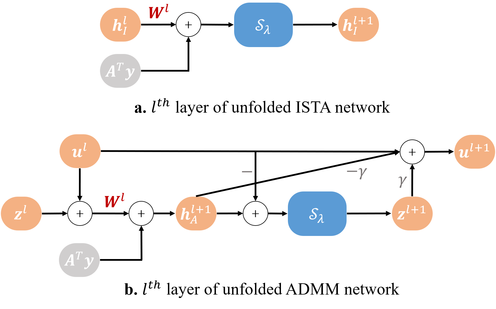
Figure 1: A single layer in the unfolded networks. a. Unfolded ISTA. b. Unfolded ADMM. The learnable parameters are the weight matrices (marked in red).

2.2 Generalization and Estimation Errors

In this work, we focus on upper bounding the GE and EE of the model-based neural networks of Fig. 1. The GE of a class of estimation functions $\bm{h}\in{\bm{\mathcal{H}}}$, such that $\bm{h}:\mathbb{R}^{n_{y}}\xrightarrow[]{}\mathbb{R}^{n_{x}}$, is defined as

$${\mathcal{G}}({\bm{\mathcal{H}}})={\mathbb{E}}_{S}\sup_{\bm{h}\in{\bm{\mathcal{H}}}}L_{{\mathcal{D}}}(\bm{h})-L_{S}(\bm{h})$$ (6)

where $L_{{\mathcal{D}}}(\bm{h})={\mathbb{E}}_{{\mathcal{D}}}{\mathcal{L}}(\bm{h})$ is the expected loss with respect to the data distribution ${\mathcal{D}}$ (the joint probability distribution of the targets and observations), $L_{S}(\bm{h})=\frac{1}{m}\sum_{i=1}^{m}{\mathcal{L}}(\bm{h}(\bm{y}_{i}),\bm{x}_{i})$ is the average empirical loss with respect to the training set $\mathcal{S}$, and ${\mathbb{E}}_{S}$ is the expectation over the training datasets. The GE is a global property of the class of estimators, which captures how the class of estimators ${\bm{\mathcal{H}}}$ is suited to the learning problem. Large GE implies that there are hypotheses in ${\bm{\mathcal{H}}}$ for which $L_{D}$ deviates much from $L_{S}$, on average over $S$. However, the GE in (6) does not capture how the learning algorithm chooses the estimator $\bm{h}\in{\bm{\mathcal{H}}}$.

In order to capture the effect of the learning algorithm, we consider local properties of the class of estimators, and focus on bounding the estimation error (EE)

$${\mathcal{E}}({\bm{\mathcal{H}}})=L_{{\mathcal{D}}}\left(\bm{\hat{h}}\right)-\inf_{\bm{h}\in{\bm{\mathcal{H}}}}L_{{\mathcal{D}}}\left(\bm{h}\right)$$ (7)

where $\bm{\hat{h}}$ is the ERM satisfying $L_{S}(\bm{\hat{h}})=\inf_{\bm{h}\in{\bm{\mathcal{H}}}}L_{{\mathcal{S}}}(\bm{h})$. We note that the ERM approximates the learned estimator $\bm{h}_{\textit{learned}}$, which is obtained by training the network on a set of training examples $S$, using algorithms such as SGD. However, the estimator $\bm{h}_{\textit{learned}}$ depends on the optimization algorithm, and can differ from the ERM. The difference between the empirical loss associated with $\bm{\hat{h}}$ and the empirical loss associated with $\bm{h}_{\textit{learned}}$ is usually referred to as the optimization error.

Common deep neural network architectures have large GE compared to the low EE achieved in practice. This still holds, when the networks are not trained with explicit regularization, such as weight decay, early stopping, or drop-outs (Srivastava et al., 2014; Neyshabur et al., 2015b). This empirical phenomena is experienced across various architectures and hyper-parameter choices (Liang et al., 2019; Novak et al., 2018; Lee et al., 2018; Neyshabur et al., 2018).

2.3 Rademacher Complexity based Bounds

The RC is a standard tool which captures the ability of a class of functions to approximate noise, where a lower complexity indicates a reduced generalization error. Formally, the empirical RC of a class of scalar estimators ${\mathcal{H}}$, such that $h:\mathbb{R}^{n_{y}}\xrightarrow[]{}\mathbb{R}$ for $h\in{\mathcal{H}}$, over $m$ samples is

$$\mathfrak{R}_{m}\left({{\mathcal{H}}}\right)={\mathbb{E}}_{\{\epsilon_{i}\}_{i=1}^{m}}\sup_{h\in{\mathcal{H}}}\frac{1}{m}\sum_{i=1}^{m}\epsilon_{i}h(\bm{y}_{i})$$ (8)

where $\{\epsilon_{i}\}_{i=1}^{m}$ are independent Rademacher random variables for which $Pr\left(\epsilon_{i}=1\right)=Pr\left(\epsilon_{i}=-1\right)=1/2$, the samples $\{\bm{y}_{i}\}_{i=1}^{m}$ are obtained by the model in (1) from $m$ i.i.d. target vectors $\{\bm{x}_{i}\}_{i=1}^{m}$ drawn from an unknown distribution. Taking the expectation of the RC of ${{\mathcal{L}}}\circ{{\bm{\mathcal{H}}}}$ with respect to the set of examples $S$ presented in Section 2.1, leads to a bound on the GE

$${\mathcal{G}}({\bm{\mathcal{H}}})\leq 2{\mathbb{E}}_{S}\mathfrak{R}_{m}\left({{{\mathcal{L}}}\circ{{\bm{\mathcal{H}}}}}\right)$$ (9)

where ${\mathcal{L}}$ is defined in Section 2.1 and ${{\mathcal{L}}}\circ{{\bm{\mathcal{H}}}}=\left\{(\bm{x},\bm{y})\mapsto{\mathcal{L}}(h(\bm{y}),\bm{x}):h\in{\bm{\mathcal{H}}}\right\}$ (Shalev-Shwartz & Ben-David, 2014). We observe that the class of functions ${{\mathcal{L}}}\circ{{\bm{\mathcal{H}}}}$ consists of scalar functions, such that $f:\mathbb{R}^{n_{x}}\times\mathbb{R}^{n_{x}}\xrightarrow[]{}\mathbb{R}$ for $f\in{{\mathcal{L}}}\circ{{\bm{\mathcal{H}}}}$. Therefore, in order to bound the GE of the class of functions defined by ISTA and ADMM networks, we can first bound their RC.

Throughout the paper, we compare the model-based architectures with a feed forward network with ReLU activations, given by $\textit{ReLU}(\bm{h})=\max\left(\bm{h},\bm{0}\right)$. In this section, we review existing bounds for the generalization error of these networks. The layers of a ReLU network $\bm{h}_{R}^{l},\ \forall l\in[1,L]$, are defined by the following recurrence relation $\bm{h}_{R}^{l}=\textit{ReLU}\left(\bm{W}^{l}\bm{h}_{R}^{l-1}+\bm{b}\right)$, and $\bm{h}_{R}^{0}=\textit{ReLU}(\bm{b}),$ where $\bm{W}^{l},\ \forall l\in[1,L]$ are the weight matrices which satisfy the same conditions as the weight matrices of ISTA and ADMM networks. The class of functions representing the output at depth $L$ in a ReLU network, is ${\bm{\mathcal{H}}}_{R}^{L}=\{\bm{h}_{R}^{L}(\{\bm{W}^{l}\}_{l=1}^{L}):||\bm{W}^{l}||_{\infty}\leq B_{l}\ l\in[1,L],\ ||\bm{W}^{1}||_{2}\leq B_{1}\}$. This architecture leads to the following bound on the GE.

Theorem 1 (Generalization error bound for ReLU networks (Gao & Zhou, 2016)).

Consider the class of feed forward networks of depth-$L$ with ReLU activations, ${\bm{\mathcal{H}}}_{R}^{L}$, as described in Section 2.3, and $m$ i.i.d. training samples. Given a $1$-Lipschitz loss function, its GE satisfies ${\mathcal{G}}{\left({\bm{\mathcal{H}}}_{R}^{L}\right)}\leq 2G^{l}_{R}$, where $G^{l}_{R}=\frac{B_{0}\prod_{l=1}^{L}B_{l}}{\sqrt{m}}$.

Proof.

Follows from applying the bound of the RC of ReLU neural networks from (Gao & Zhou, 2016) and combining it with (9). ∎

The bound in Theorem 1 is satisfied for any feed forward network with $1$-Lipschitz nonlinear activations (including ReLU), and can be generalized for networks with activations with different Lipshcitz constants. We show in Theorem 2, that the bound presented in Theorem 1 cannot be substantially improved for ReLU networks with the RC framework.

Theorem 2 (Lower Rademacher complexity bound for ReLU networks (Bartlett et al., 2017)).

Consider the class of feed forward networks of depth-$L$ with ReLU activations, where the weight matrices have bounded spectral norm $||\bm{W}^{l}||_{\sigma}\leq B^{\prime}_{l},\ l\in[1,L]$. The dimension of the output layer is $1$, and the dimension of each non-output layer is at least $2$. Given $m$ i.i.d. training samples, there exists a $c$ such that $\mathfrak{R}_{m}\left({{\mathcal{H}}^{\prime,L}_{R}}\right)\geq cB_{0}\prod_{l=1}^{L}B^{\prime}_{l}$, where ${\mathcal{H}}_{R}^{\prime,L}=\{h_{R}^{L}(\{\bm{W}^{l}\}_{l=1}^{L}):||\bm{W}^{l}||_{\sigma}\leq B^{\prime}_{l}\ \,l\in[1,L]\}$.

This result shows that using the RC framework the GE of ReLU networks behaves as the product of the weight matrices’ norms $\prod_{l=1}^{L}B_{l}$, as captured in Theorem 1. Theorem 2, implies that the dependence on the weight matrices’ norms, cannot be substantially improved with the RC framework for ReLU networks.

3 Generalization Error Bounds: Global Properties

In this section, we derive theoretical bounds on the GE of learned ISTA and ADMM networks. From these bounds we deduce design rules to construct ISTA and ADMM networks with a GE which does not increase exponentially with the number of layers. We start by presenting theoretical guarantees on the RC of any class of functions, after applying the soft-thresholding operation.

Soft-thresholding is a basic block that appears in multiple iterative algorithms, and therefore is used as the nonlinear activation in many model-based networks. It results from the proximal gradient of the $L_{1}$ norm (Palomar & Eldar, 2010). We therefore start by presenting the following lemma which expresses how the RC of a class of functions is affected by applying soft-thresholding to each function in the class. The proof is provided in the supplementary material.

Lemma 1 (Rademacher complexity of soft-thresholding).

Given any class of scalar functions ${\mathcal{H}}$ where $h:\mathbb{R}^{n}\xrightarrow[]{}\mathbb{R},\ h\in{\mathcal{H}}$ for any integer $n\geq 1$, and $m$ i.i.d. training samples,

$$\mathfrak{R}_{m}\left({{S_{\lambda}}\circ{{\mathcal{H}}}}\right)\leq\mathfrak{R}_{m}\left({{\mathcal{H}}}\right)-\frac{\lambda T}{m},$$ (10)

where $T=\sum_{i=1}^{m}T_{i}$ and $T_{j}={\mathbb{E}}_{\{\epsilon_{i}\}_{i=2}^{m}}\left(\mathbbm{1}_{h^{\star}(\bm{y}_{j})>\lambda\land h^{\prime\star}(\bm{y}_{j})<-\lambda}\right)$ such that $h^{*},\,h^{\prime*}=\operatorname*{arg\,max}_{h,h^{\prime}\in{\mathcal{H}}}\left(h(\bm{y}_{1})-h^{\prime}(\bm{y}_{1})-2\lambda\mathbbm{1}_{h(\bm{y}_{1})>\lambda\land h^{\prime}(\bm{y}_{1})<-\lambda}+\sum_{i=2}^{m}\epsilon_{i}({\mathcal{S}}_{\lambda}(h(\bm{y}_{i}))+{\mathcal{S}}_{\lambda}(h^{\prime}(\bm{y}_{i})))\right).$

The quantity $T$ is a non-negative value obtained during the proof, which depends on the networks’ number of layers, underlying data distribution ${\mathcal{D}}$ and soft-threshold value $\lambda$. As seen from (10), the value of $T$ dictates the reduction in RC due to soft-thresholding, where a reduction in the RC can also be expected. The value of $T$ increases as $\lambda$ decreases. In the case that $\lambda T$ increases with $\lambda$, higher values of $\lambda$ further reduce the RC of the class of functions ${\mathcal{H}}$, due to the soft-thresholding.

We now focus on the class of functions representing the output of a neuron at depth $L$ in an ISTA network, ${\bm{\mathcal{H}}}_{I}^{L}$. In the following theorem, we bound its GE using the RC framework and Lemma 1. The proof is provided in the supplementary material.

Theorem 3 (Generalization error bound for ISTA networks).

Consider the class of learned ISTA networks of depth $L$ as described in (2), and $m$ i.i.d. training samples. Then there exist $T^{(l)}$ for $\ l\in[1,L]$ in the range $T^{(l)}\in\left[0,\min\left\{\frac{mB_{l}G_{I}^{l-1}}{\lambda},m\right\}\right]$ such that ${\mathcal{G}}{\left({\bm{\mathcal{H}}}_{I}^{L}\right)}\leq 2{\mathbb{E}}_{S}G_{I}^{L}$, where

$$G_{I}^{l}=\left(\frac{B_{0}\prod_{l^{\prime}=1}^{l}B_{l^{\prime}}}{\sqrt{m}}-\frac{\lambda}{m}\sum_{l^{\prime}=1}^{l-1}T^{(l^{\prime})}\prod_{j=l^{\prime}+1}^{l}B_{j}-\frac{\lambda T^{(l)}}{m}\right).$$ (11)

Next, we show that for a specific distribution, the expected value of $T^{(l)}$ is greater than $0$. Under an additional bound on the expectation value of the estimators (specified in the supplementary material)

$$\mathbb{E}_{S}\left(T^{(l)}\right) \geq\max\left\{m\left(1-2e^{-(cB_{l}b^{(l)}-\lambda)}\right),0\right\}$$ (12)

where $b^{(l+1)}=B_{l}b^{(l)}-\lambda$, $b^{(1)}=B_{0}$, and $c\in(0,1]$. Increasing $\lambda$ or decreasing $B$, will decrease the bound in (12), since crossing the threshold is less probable. Depending on $\lambda$ and $\{B_{l}\}_{l=1}^{L}$ (specifically that $\lambda\leq cB_{l}b^{(l)}+\ln 2$), the bound in (12) is positive, and enforces a non-zero reduction in the GE. Along with Theorem 3, this shows the expected reduction in GE of ISTA networks compared to ReLU netowrks. The reduction is controlled by the value of the soft threshold.

To obtain a more compact relation, we can choose the maximal matrices’ norm $B=\max_{l\in[1,L]}B_{l}$, and denote $T=\min_{l\in[1,L]}T^{(l)}\in[0,m]$ which leads to ${\mathcal{G}}{\left({\bm{\mathcal{H}}}_{I}^{L}\right)}\leq 2\left(\frac{B_{0}B^{L}}{\sqrt{m}}-\frac{\lambda{\mathbb{E}}_{S}(T)}{m}\frac{B^{L}-1}{B-1}\right).$

Comparing this bound with the GE bound for ReLU networks presented in Theorem 1, shows the expected reduction due to the soft thresholding activation. This result also implies practical rules for designing low generalization error ISTA networks. We note that the network’s parameters such as the soft-threshold value $\lambda$ and number of samples $m$, are predefined by the model being solved (for example, in ISTA, the value of $\lambda$ is chosen according to the singular values of $\bm{A}$).

We derive an implicit design rule from (3), for a nonincreasing GE, as detailed in Section A.2. This is done by restricting the matrices’ norm to satisfy $B\leq 1+\frac{\lambda{\mathbb{E}}_{S}(T)}{\sqrt{m}B_{0}}$. Moreover, these results can be extended to convolutional neural networks. As convolution operations can be expressed via multiplication with a convolution matrix, the presented results are also satisfied in that case.

Similarly, we bound the GE of the class of functions representing the output at depth $L$ in an ADMM network, ${\mathcal{H}}_{A}^{L}$. The proof and discussion are provided in the supplementary material.

Theorem 4 (Generalization error bound for ADMM networks).

Consider the class of learned ADMM networks of depth $L$ as described in (4), and $m$ i.i.d. training samples. Then there exist $T^{(l)}$ for $l\in[1,L-1]$ in the interval $T^{(l)}\in\left[0,\min\left\{\frac{m\tilde{B}_{l}G_{A}^{l-1}}{\tilde{\lambda}},m\right\}\right]$ where $G_{A}^{l}=\frac{B_{0}\prod_{l^{\prime}=1}^{l-1}\tilde{B_{l^{\prime}}}}{\sqrt{m}}-\frac{\tilde{\lambda}}{m}\sum_{l^{\prime}=1}^{l-2}T^{(l^{\prime})}\prod_{j=l^{\prime}+1}^{l-1}\tilde{B}_{j}-\frac{\tilde{\lambda}T^{(l-1)}}{m}$, and $\tilde{\lambda}=(1+\gamma)\lambda$, $\tilde{B}_{l}=(1+2\gamma)(B_{l}+2),\ l\in[1,L]$, such that ${\mathcal{G}}\left({\bm{\mathcal{H}}}_{A}^{L}\right)\leq 2\tilde{B}_{L}{\mathbb{E}}_{S}G_{A}^{L-1}.$

We compare the GE bounds for ISTA and ADMM networks, to the bound on the GE of ReLU networks presented in Theorem 1. We observe that both model-based networks achieve a reduction in the GE, which depends on the soft-threshold, the underlying data distribution, and the bound on the norm of the weight matrices. Following the bound, we observe that the soft-thresholding nonlinearity is most valuable in the case of small number of training samples. The soft-thresholding nonlinearity is the key that enables reducing the GE of the ISTA and ADMM networks compared to ReLU networks. Next, we focus on bounding the EE of feed-forward networks based on the LRC framework.

4 Estimation Error Bounds: Local Properties

To investigate the model-based networks’ EE, we use the LRC framework (Bartlett et al., 2005). Instead of considering the entire class of functions ${\bm{\mathcal{H}}}$, the LRC considers only estimators which are close to the optimal estimator ${\bm{\mathcal{H}}}_{r}=\left\{\bm{h}\in{\bm{\mathcal{H}}}:{\mathbb{E}}_{{\mathcal{D}}}\left\|{\bm{h}(\bm{y})-\bm{h}^{*}(\bm{y})}\right\|^{2}_{2}\leq r\right\}$, where $\bm{h}^{*}$ is such that $L_{D}(\bm{h}^{*})=\inf_{\bm{h}\in{\bm{\mathcal{H}}}}L_{{\mathcal{D}}}(\bm{h})$. It is interesting to note that the class of estimators ${\bm{\mathcal{H}}}_{r}$ only restricts the distance between the estimators themselves, and not between their corresponding losses. Following the LRC framework, we consider target vectors ranging in $[-1,1]^{n_{x}}$. Therefore, we adapt the networks’ estimations by clipping them to lie in the interval $[-1,1]^{n_{x}}$. In our case we consider the restricted classes of functions representing the output of a neuron at depth $L$ in ISTA, ADMM, and ReLU networks. Moreover, we denote by $\bm{W}^{l}$ and $\bm{W}^{l,*},\ l\in[1,L]$ the weight matrices corresponding to $\bm{h}\in{\bm{\mathcal{H}}}_{r}$ and $\bm{h}^{*}$, respectively. Based on these restricted class of functions, we present the following assumption and theorem (the proof is provided in the supplementary material).

Assumption 1.

There exists a constant $C\geq 1$ such that for every probability distribution ${\mathcal{D}}$, and estimator $\bm{h}\in{\bm{\mathcal{H}}}$, ${\mathbb{E}}_{{\mathcal{D}}}\sum_{j=1}^{n_{x}}(\bm{h}_{j}-\bm{h}^{*}_{j})^{2}\leq C{\mathbb{E}}_{{\mathcal{D}}}\sum_{j=1}^{n_{x}}\left(\ell(\bm{h}_{j})-\ell(\bm{h}^{*}_{j})\right)$, where $\bm{h}_{j}$ and $\bm{h}^{*}_{j}$ denote the $j$th coordinate of the estimators.

As pointed out in (Bartlett & Mendelson, 2002), this condition usually follows from a uniform convexity condition on the loss function $\ell$. For instance, if $\left|h(\bm{y})-\bm{x}\right|\leq 1$ for any $h\in{\mathcal{H}},\bm{y}\in{\mathbb{R}}^{n_{y}}$ and $\bm{x}\in{\mathbb{R}}^{n_{x}}$, then the condition is satisfied with $C=1$ (Yousefi et al., 2018).

Theorem 5 (Estimation error bound of ISTA, ADMM, and ReLU networks).

Consider the class of functions represented by depth-$L$ ISTA networks ${\bm{\mathcal{H}}}_{I}^{L}$ as detailed in Section 2.1, $m$ i.i.d training samples, and a per-coordinate loss satisfying Assumption 1 with a constant $C$. Let $||\bm{W}^{l}-\bm{W}^{l,*}||_{\infty}\leq\alpha\sqrt{r}$ for some $\alpha>0$. Moreover, $B\geq\max\{\alpha\sqrt{r},1\}$. Then there exists $T$ in the interval $T\in\left[0,\min\left\{\frac{\sqrt{m}B_{0}B^{L-1}2^{L}}{\lambda\eta},m\right\}\right]$, where $\eta=\frac{LB^{L-1}(B-1)-B^{L}+1}{(B-1)^{2}}$, such that for any $s>0$ with probability at least $1-e^{-s}$,

$${\mathcal{E}}{\left({\bm{\mathcal{H}}}_{I}^{L}\right)}\leq 41r^{*}+\frac{17C^{2}+48C}{mn_{x}}s$$ (13)

where $r^{*}=C^{2}\alpha^{2}\left(\frac{B_{0}B^{L-1}2^{L}}{\sqrt{m}}-\frac{\lambda T}{m}\eta\right)^{2}$. The bound is also satisfied for the class of functions represented by depth-$L$ ADMM networks ${\bm{\mathcal{H}}}_{A}^{L}$, with $r^{*}=C^{2}\alpha^{2}\left(\frac{B_{0}\tilde{B}^{L-2}2^{L-1}}{\sqrt{m}}-\frac{\tilde{\lambda}T}{m}\tilde{\eta}\right)^{2}$, where $\tilde{\lambda}=(1+\gamma)\lambda$, $\tilde{B}=(1+2\gamma)(B+2)$, and $\tilde{\eta}=\frac{(L-1)\tilde{B}^{L-2}(\tilde{B}-1)-\tilde{B}^{L-1}+1}{(\tilde{B}-1)^{2}}$, and for the class of functions represented by depth-$L$ ReLU networks ${\bm{\mathcal{H}}}_{R}^{L}$, with $r^{*}=C^{2}\alpha^{2}\,\left(\frac{B_{0}B^{L-1}2^{L}}{\sqrt{m}}\right)^{2}$.

From Theorem 5, we observe that the EE decreases by a factor of ${\mathcal{O}}\left(1/m\right)$, instead of a factor of ${\mathcal{O}}\left(1/\sqrt{m}\right)$ obtained for the GE. This result complies with previous local bounds which yield faster convergence rates compared to global bounds (Blanchard et al., 2007; Bartlett et al., 2005). Also, the value of $\alpha$ relates the maximal distance between estimators in ${\mathcal{H}}_{r}$ denoted by $r$, to the distance between their corresponding weight matrices $||\bm{W}^{l}-\bm{W}^{l,*}||_{\infty}\leq\alpha\sqrt{r},\ l\in[1,L]$. Tighter bounds on the distance between the weight matrices allow us to choose a smaller value for $\alpha$, resulting in smaller values $r^{*}$ which improve the EE bounds. The value of $\alpha$ could depend on the network’s nonlinearity, underlying data distribution ${\mathcal{D}}$, and number of layers.

Note that the bounds of the model-based architectures depend on the soft-thresholding through the value of $\lambda{\mathbb{E}}_{S}(T)$. As $\lambda{\mathbb{E}}_{S}(T)$ increases, the bound on the EE decreases, which emphasizes the nonlinearity’s role in the network’s generalization abilities. Due to the soft-thresholding, ISTA and ADMM networks result in lower EE bounds compared to the bound for ReLU networks. It is interesting to note, that as the number of training samples $m$ increases, the difference between the bounds on the model-based and ReLU networks is less significant. In the EE bounds of model-based networks, the parameter $B_{0}$ relates the bound to the sparsity level $\rho$, of the target vectors. Lower values of $\rho$ result in lower EE bounds, as demonstrated in the supplementary.

5 Numerical Experiments

In this section, we present a series of experiments that concentrate on how a particular model-based network (ISTA network) compares to a ReLU network, and showcase the merits of model-based networks. We focus on networks with $10$ layers (similar to previous works (Gregor & LeCun, 2010)), to represent realistic model-based network architectures. The networks are trained on a simulated dataset to solve the problem in (1), with target vectors uniformly distributed in $[-1,1]$. The linear mapping $\bm{A}$ is constructed from the real part of discrete Fourier transform (DFT) matrix rows (Ong et al., 2019), where the rows are randomly chosen. The sparsity rate is $\rho=0.15$, and the noise’s standard deviation is $0.1$. To train the networks we used the SGD optimizer with the $L_{1}$ loss over all neurons of the last layer. The target and noise vectors are generated as element wise independently from a uniform distribution ranging in $[-1,1]$ . All results are reproducible through (Authors, 2022) which provides the complete code to execute the experiments presented in this section.

We concentrate on comparing the networks’ EE, since in practice, the networks are trained with a finite number of examples. In order to empirically approximate the EE of a class of networks ${\mathcal{H}}$, we use an empirical approximation of $h^{*}$ (which satisfy ${\mathcal{L}}_{{\mathcal{D}}}(h^{*})=\inf_{h\in{\mathcal{H}}}{\mathcal{L}}_{{\mathcal{D}}}(h)$) and the ERM $\hat{h}$, denoted by $h^{*}_{emp}$ and $\hat{h}_{emp}$ respectively. The estimator $h^{*}_{emp}$ results from the trained network with $10^{4}$ samples, and the ERM is approximated by a network trained using SGD with $m$ training samples (where $m\leq 10^{4}$). The empirical EE is given by their difference ${\mathcal{L}}_{{\mathcal{D}}}(\hat{h}_{emp})-{\mathcal{L}}_{{\mathcal{D}}}(h^{*}_{emp})$.

In Fig. 2, we compare between the ISTA and ReLU networks, in terms of EE and $L_{1}$ loss, for networks trained with different number of samples (between $10$ and $10^{4}$ samples). We observe that for small number of training samples, the ISTA network substantially reduces the EE compared to the ReLU network. This can be understood from Theorem 5, which results in lower EE bounds on the ISTA networks compared to ReLU networks, due to the term $\lambda{\mathbb{E}}_{S}(T)$. However, for large number of samples the EE of both networks decreases to zero, which is also expected from Theorem 5. This highlights that the contribution of the soft-thresholding nonlinearity to the generalization abilities of the network is more significant for small number of training samples. Throughout the paper, we considered networks with constant bias terms. In this section, we also consider learned bias terms, as detailed in the supplementary material. In Fig. 2, we present the experimental results for networks with constant and learned biases. The experiments indicate that the choice of constant or learned bias is less significant to the EE or the accuracy, compared to the choice of nonlinearity, emphasizing the relevance of the theoretical guarantees. The cases of learned and constant biases have different optimal estimators, as the networks with learned biases have more learned parameters. As a result, it is plausible a network with more learnable parameters (the learnable bias) exhibits a lower estimation error since the corresponding optimal estimator also exhibits a lower estimation error.

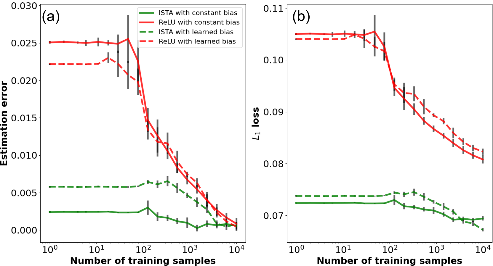
Figure 2: Comparing the EE of ISTA and ReLU networks with $10$ layers. a. The EE of the networks as a function of the training samples. b. The $L_{1}$ of the networks as a function of the training samples. The ISTA network achieves lower EE compared to the ReLU network, along with lower losses.

To analyze the effect of the soft-thresholding value on the generalization abilities of the ISTA network, we show in Fig. 3, the empirical EE for multiple values of $\lambda$. The experimental results demonstrate that for small number of samples, increasing $\lambda$ reduces the EE. As expected from the EE bounds, for a large number of training samples, this dependency on the nonlinearity vanishes, and the EE is similar for all values of $\lambda$. In Fig. 3b, we show the $L_{1}$ loss of the ISTA networks for different values of $\lambda$. We observe that low estimation error does not necessarily lead to low loss value. For $m\lesssim 100$, increasing $\lambda$ reduced the EE. These results suggest that given ISTA networks with different values of $\lambda$ such that all networks achieve similar accuracy, the networks with higher values of $\lambda$ provide lower EE. These results are also valid for additional networks’ depths. In Section B, we compare the EE for networks with different number of layers, and show that they exhibit a similar behaviour.

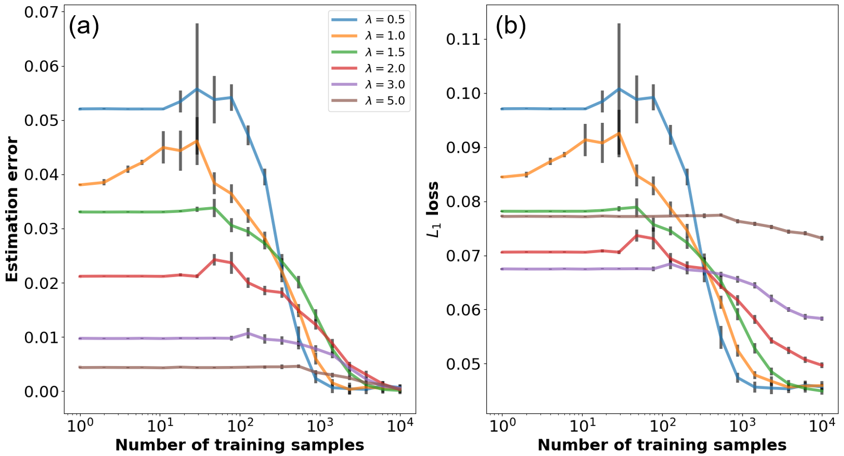
Figure 3: Estimation error and loss of ISTA networks with $10$ layers, as a function of the soft-threshold’s value $\lambda$. The experiments indicate that the estimation error decreases as $\lambda$ increases, which demonstrates a way to control the networks’ generalization abilities through $\lambda$.

6 Conclusion

We derived new GE and EE bounds for ISTA and ADMM networks, based on the RC and LRC frameworks. Under suitable conditions, the model-based networks’ GE is nonincreasing with depth, resulting in a substantial improvement compared to the GE bound of ReLU networks. The EE bounds explain EE behaviours experienced in practice, such as ISTA networks demonstrating higher estimation abilities, compared to ReLU networks, especially for small number of training samples. Through a series of experiments, we show that the generalization abilities of ISTA networks are controlled by the soft-threshold value, and achieve lower EE along with a more accurate recovery compared to ReLU networks which increase the GE and EE with the networks’ depths.

It is interesting to consider how the theoretical insights can be harnessed to enforce neural networks with high generalization abilities. One approach is to introduce an additional regularizer during the training process that is rooted in the LRC, penalizing networks with high EE (Yang et al., 2019).

Appendix A Supplementary Material

In this supplementary material we provide the proofs of the presented lemmas and theorems.

A.1 Rademacher complexity of the soft-thresholding operator

In this section, we prove Lemma 1 which examines how the RC is affected by the soft-thresholding operator.

Lemma 1 (Rademacher complexity of soft-thresholding):
Given any class of scalar functions ${\mathcal{H}}$ where $h:\mathbb{R}^{n}\xrightarrow[]{}\mathbb{R},\ h\in{\mathcal{H}}$ for any integer $n\geq 1$, there exists a value $T$ in the interval

$$T\in\left(0,\min\left\{\frac{m\mathfrak{R}_{m}\left({{\mathcal{H}}}\right)}{\lambda},m\right\}\right]$$ (14)

such that

$$\mathfrak{R}_{m}\left({{S_{\lambda}}\circ{{\mathcal{H}}}}\right)\leq\mathfrak{R}_{m}\left({{\mathcal{H}}}\right)-\frac{\lambda T}{m}.$$ (15)

Proof.

We start by denoting

$$R=m\mathfrak{R}_{m}\left({{S_{\lambda}}\circ{{\mathcal{H}}}}\right)={\mathbb{E}}_{\{\epsilon_{i}\}_{i=1}^{m}}\sup_{h\in{\mathcal{H}}}\sum_{i=1}^{m}\epsilon_{i}{\mathcal{S}}_{\lambda}(h(\bm{y}_{i}))$$ (16)

and we explicitly compute the expectation on $\epsilon_{1}$:

$$R={\mathbb{E}}_{\{\epsilon_{i}\}_{i=1}^{m}} \sup_{h\in{\mathcal{H}}}\sum_{i=1}^{m}\epsilon_{i}{\mathcal{S}}_{\lambda}(h(\bm{y}_{i}))$$ (17)

$$={\mathbb{E}}_{\{\epsilon_{i}\}_{i=1}^{m}} \sup_{h\in{\mathcal{H}}}\epsilon_{1}{\mathcal{S}}_{\lambda}(h(\bm{y}_{1}))+\sum_{i=2}^{m}\epsilon_{i}{\mathcal{S}}_{\lambda}(h(\bm{y}_{i}))$$

$$={\mathbb{E}}_{\{\epsilon_{i}\}_{i=2}^{m}} \left[\frac{1}{2}\sup_{h\in{\mathcal{H}}}\left({\mathcal{S}}_{\lambda}(h(\bm{y}_{1}))+\sum_{i=2}^{m}\epsilon_{i}{\mathcal{S}}_{\lambda}(h(\bm{y}_{i}))\right)+\frac{1}{2}\sup_{h^{\prime}\in{\mathcal{H}}}\left(-{\mathcal{S}}_{\lambda}(h^{\prime}(\bm{y}_{1}))+\sum_{i=2}^{m}\epsilon_{i}{\mathcal{S}}_{\lambda}(h^{\prime}(\bm{y}_{i}))\right)\right]$$

$$=\frac{1}{2}{\mathbb{E}}_{\{\epsilon_{i}\}_{i=2}^{m}} \sup_{h\in{\mathcal{H}}}\left({\mathcal{S}}_{\lambda}(h(\bm{y}_{1}))+\sum_{i=2}^{m}\epsilon_{i}{\mathcal{S}}_{\lambda}(h(\bm{y}_{i}))\right)+\sup_{h^{\prime}\in{\mathcal{H}}}\left(-{\mathcal{S}}_{\lambda}(h^{\prime}(\bm{y}_{1}))+\sum_{i=2}^{m}\epsilon_{i}{\mathcal{S}}_{\lambda}(h^{\prime}(\bm{y}_{i}))\right)$$

$$=\frac{1}{2}{\mathbb{E}}_{\{\epsilon_{i}\}_{i=2}^{m}} \sup_{h,h^{\prime}\in{\mathcal{H}}}\left({\mathcal{S}}_{\lambda}(h(\bm{y}_{1}))-{\mathcal{S}}_{\lambda}(h^{\prime}(\bm{y}_{1}))+\sum_{i=2}^{m}\epsilon_{i}({\mathcal{S}}_{\lambda}(h(\bm{y}_{i}))+{\mathcal{S}}_{\lambda}(h^{\prime}(\bm{y}_{i})))\right).$$

To simplify the notations, we denote

$$s_{\bm{\epsilon}}({h},{h^{\prime}}) =\sum_{i=2}^{m}\epsilon_{i}({\mathcal{S}}_{\lambda}(h(\bm{y}_{i}))+{\mathcal{S}}_{\lambda}(h^{\prime}(\bm{y}_{i})))$$ (18)

and observe that $s_{\bm{\epsilon}}({h},{h^{\prime}})=s_{\bm{\epsilon}}({h^{\prime}},{h})$.

Next, we show that the soft-thresholding on the estimations of the first sample, reduces the RC, and results in

$$R\leq\frac{1}{2}{\mathbb{E}}_{\{\epsilon_{i}\}_{i=2}^{m}} \sup_{h,h^{\prime}\in{\mathcal{H}}}\left(h(\bm{y}_{1})-h^{\prime}(\bm{y}_{1})-2\lambda\mathbbm{1}_{h(\bm{y}_{1})>\lambda\land h^{\prime}(\bm{y}_{1})<-\lambda}+s_{\bm{\epsilon}}({h},{h^{\prime}})\right).$$ (19)

The soft-thresholding function is piecewise linear with three pieces, and can be written as

$${\mathcal{S}}_{\lambda}(x)=\begin{cases}x+\lambda,&x<-\lambda\\ 0,&x\in[-\lambda,\lambda]\\ x-\lambda,&x>\lambda\end{cases}.$$ (20)

We focus on the terms $h(\bm{y}_{1})$ and $h^{\prime}(\bm{y}_{1})$, in the different regions determined by (20). To capture these regions, we define the following classes of functions

$${\mathcal{H}}^{-1} =\left\{h\in{\mathcal{H}}:h(\bm{y}_{1})<-\lambda\right\}$$ (21)

$${\mathcal{H}}^{0} =\left\{h\in{\mathcal{H}}:h(\bm{y}_{1})\in[-\lambda,\lambda]\right\}$$

$${\mathcal{H}}^{1} =\left\{h\in{\mathcal{H}}:h(\bm{y}_{1})>\lambda\right\}.$$

We can then write

$$r=\max_{\alpha,\beta\in\{-1,0,1\}}r_{\alpha,\beta}$$ (22)

where

$$r_{\alpha,\beta}=\sup_{h\in{\mathcal{H}}^{\alpha},h^{\prime}\in{\mathcal{H}}^{\beta}}\left({\mathcal{S}}_{\lambda}(h(\bm{y}_{1}))-{\mathcal{S}}_{\lambda}(h^{\prime}(\bm{y}_{1}))+s_{\bm{\epsilon}}({h},{h^{\prime}})\right).$$ (23)

We now divide into cases for the different values of $\alpha$ and $\beta$:

1. For $\alpha,\beta=1$ or $\alpha,\beta=-1$, we obtain that ${\mathcal{S}}_{\lambda}(h(\bm{y}_{1}))-{\mathcal{S}}_{\lambda}(h^{\prime}(\bm{y}_{1}))=h(\bm{y}_{1})-h^{\prime}(\bm{y}_{1})$. As a result,

   $$r_{1,1}=\sup_{h\in{\mathcal{H}}^{1},h^{\prime}\in{\mathcal{H}}^{1}}\left(h(\bm{y}_{1})-h^{\prime}(\bm{y}_{1})+s_{\bm{\epsilon}}({h},{h^{\prime}})\right)$$ (24)

   and

   $$r_{-1,-1}=\sup_{h\in{\mathcal{H}}^{-1},h^{\prime}\in{\mathcal{H}}^{-1}}\left(h(\bm{y}_{1})-h^{\prime}(\bm{y}_{1})+s_{\bm{\epsilon}}({h},{h^{\prime}})\right).$$ (25)

2. For $\alpha=1$ and $\beta=0$, we obtain that ${\mathcal{S}}_{\lambda}(h(\bm{y}_{1}))-{\mathcal{S}}_{\lambda}(h^{\prime}(\bm{y}_{1}))=h(\bm{y}_{1})-\lambda$. In this case, $h^{\prime}(\bm{y}_{1})\leq\lambda$, which results in

   $$r_{1,0} =\sup_{h\in{\mathcal{H}}^{1},h^{\prime}\in{\mathcal{H}}^{0}}\left(h(\bm{y}_{1})-\lambda+s_{\bm{\epsilon}}({h},{h^{\prime}})\right)$$ (26)

   $$\leq\sup_{h\in{\mathcal{H}}^{1},h^{\prime}\in{\mathcal{H}}^{0}}\left(h(\bm{y}_{1})-h^{\prime}(\bm{y}_{1})+s_{\bm{\epsilon}}({h},{h^{\prime}})\right).$$

3. For $\alpha=0$ and $\beta=-1$, we obtain that ${\mathcal{S}}_{\lambda}(h(\bm{y}_{1}))-{\mathcal{S}}_{\lambda}(h^{\prime}(\bm{y}_{1}))=-h^{\prime}(\bm{y}_{1})-\lambda$. In this case, $h(\bm{y}_{1})\geq-\lambda$, which results in

   $$r_{0,-1} =\sup_{h\in{\mathcal{H}}^{0},h^{\prime}\in{\mathcal{H}}^{-1}}\left(-h^{\prime}(\bm{y}_{1})-\lambda+s_{\bm{\epsilon}}({h},{h^{\prime}})\right)$$ (27)

   $$\leq\sup_{h\in{\mathcal{H}}^{0},h^{\prime}\in{\mathcal{H}}^{-1}}\left(h(\bm{y}_{1})-h^{\prime}(\bm{y}_{1})+s_{\bm{\epsilon}}({h},{h^{\prime}})\right).$$

4. For $\alpha=1$ and $\beta=-1$, we obtain that ${\mathcal{S}}_{\lambda}(h(\bm{y}_{1}))-{\mathcal{S}}_{\lambda}(h^{\prime}(\bm{y}_{1}))=h(\bm{y}_{1})-h^{\prime}(\bm{y}_{1})-2\lambda$, which results in

   $$r_{1,-1} =\sup_{h\in{\mathcal{H}}^{1},h^{\prime}\in{\mathcal{H}}^{-1}}\left(h(\bm{y}_{1})-h^{\prime}(\bm{y}_{1})-2\lambda+s_{\bm{\epsilon}}({h},{h^{\prime}})\right).$$ (28)

   In this case, we obtain a reduction by $2\lambda$ in the complexity.

5. For $\alpha,\beta=0$, we obtain that ${\mathcal{S}}_{\lambda}(h(\bm{y}_{1}))-{\mathcal{S}}_{\lambda}(h^{\prime}(\bm{y}_{1}))=0$, which leads to

   $$r_{0,0}=\sup_{h\in{\mathcal{H}}^{0},h^{\prime}\in{\mathcal{H}}^{0}}s_{\bm{\epsilon}}({h},{h^{\prime}}).$$ (29)

   We bound this term to obtain a similar expression to the previous cases. Any pair of estimators $h,h^{\prime}\in{\mathcal{H}}^{0}$ satisfies that $h(\bm{y}_{1})\geq h^{\prime}(\bm{y}_{1})$ or $h(\bm{y}_{1})\leq h^{\prime}(\bm{y}_{1})$. Using the fact that $s_{\bm{\epsilon}}({h},{h^{\prime}})=s_{\bm{\epsilon}}({h^{\prime}},{h})$, there exists a pair $h,h^{\prime}\in{\mathcal{H}}^{0}$ satisfying $h(\bm{y}_{1})-h^{\prime}(\bm{y}_{1})+s_{\bm{\epsilon}}({h},{h^{\prime}})\geq s_{\bm{\epsilon}}({h},{h^{\prime}})$ (otherwise, interchanging between the estimators satisfies this requirement since $h^{\prime}(\bm{y}_{1})-h(\bm{y}_{1})+s_{\bm{\epsilon}}({h},{h^{\prime}})\geq s_{\bm{\epsilon}}({h},{h^{\prime}})=s_{\bm{\epsilon}}({h^{\prime}},{h})$, where the estimators satisfy $h^{\prime},h\in{\mathcal{H}}^{0}$). This means that the term $r_{0,0}$ is bounded by

   $$r_{0,0}\leq\sup_{h\in{\mathcal{H}}^{0},h^{\prime}\in{\mathcal{H}}^{0}}\left(h(\bm{y}_{1})-h^{\prime}(\bm{y}_{1})+s_{\bm{\epsilon}}({h},{h^{\prime}})\right).$$ (30)

We will now show that the additional cases that were not presented above, are dominated by other cases (i.e. upper bounded), and therefore will not be considered in (22):

1. For $\alpha=-1$ and $\beta=1$, we obtain that ${\mathcal{S}}_{\lambda}(h(\bm{y}_{1}))-{\mathcal{S}}_{\lambda}(h^{\prime}(\bm{y}_{1}))=h(\bm{y}_{1})-h^{\prime}(\bm{y}_{1})+2\lambda$, which results in:

   $$r_{-1,1} =\sup_{h\in{\mathcal{H}}^{-1},h^{\prime}\in{\mathcal{H}}^{1}}\left(h(\bm{y}_{1})-h^{\prime}(\bm{y}_{1})+2\lambda+s_{\bm{\epsilon}}({h},{h^{\prime}})\right).$$ (31)

   We now show that $r_{-1,1}\leq r_{1,-1}$, and therefore the case of $\alpha=-1$ and $\beta=1$ is upper bounded by the case of $\alpha=1$ and $\beta=-1$. For any pair of estimators in $h\in{\mathcal{H}}^{-1}$ and $h^{\prime}\in{\mathcal{H}}^{1}$, there exists a pair of estimators in $h\in{\mathcal{H}}^{1}$ and $h^{\prime}\in{\mathcal{H}}^{-1}$, which achieve a higher value (showing that $r_{-1,1}\leq r_{1,-1}$). Since we consider the case where $\alpha=-1$ and $\beta=1$, there exist $\delta(h),\delta^{\prime}(h^{\prime})>0$ such that $h(\bm{y}_{1})=-\delta(h)-\lambda$ and $h^{\prime}(\bm{y}_{1})=\delta^{\prime}(h^{\prime})+\lambda$, resulting in:

   $$r_{-1,1}=\sup_{h\in{\mathcal{H}}^{-1},h^{\prime}\in{\mathcal{H}}^{1}}c_{-1,1}(h,h^{\prime})$$ (32)

   where

   $$c_{-1,1}(h,h^{\prime}) =-\delta(h)-\delta^{\prime}(h^{\prime})+s_{\bm{\epsilon}}({h},{h^{\prime}}).$$ (33)

   Similarly, for the case of $\alpha=1$ and $\beta=-1$, we can write

   $$r_{1,-1}=\sup_{h\in{\mathcal{H}}^{1},h^{\prime}\in{\mathcal{H}}^{-1}}c_{1,-1}(h,h^{\prime})$$ (34)

   such that

   $$c_{1,-1}(h,h^{\prime}) =\lambda+\delta(h)+\lambda+\delta^{\prime}(h^{\prime})-2\lambda+s_{\bm{\epsilon}}({h},{h^{\prime}})$$ (35)

   $$=\delta(h)+\delta^{\prime}(h^{\prime})+s_{\bm{\epsilon}}({h},{h^{\prime}}).$$

   Since $s_{\bm{\epsilon}}({h^{\prime}},{h})=s_{\bm{\epsilon}}({h},{h^{\prime}})$, for any estimators $h_{-1}=-\delta_{-1}(h_{-1})-\lambda\in{\mathcal{H}}^{-1}$ and $h_{1}=\delta_{1}(h_{1})+\lambda\in{\mathcal{H}}^{1}$

   $$c_{1,-1}(h_{1},h_{-1}) =\delta_{1}(h_{1})+\delta_{2}(h_{-1})+s_{\bm{\epsilon}}({h_{1}},{h_{-1}})$$ (36)

   $$\geq-\delta_{1}(h_{1})-\delta_{2}(h_{-1})+s_{\bm{\epsilon}}({h_{-1}},{h_{1}})$$

   $$=c_{-1,1}(h_{-1},h_{1})$$

   implying that

   $$r_{-1,1}=\sup_{h\in{\mathcal{H}}^{-1},h^{\prime}\in{\mathcal{H}}^{1}}c_{-1,1}(h,h^{\prime})\leq\sup_{h^{\prime}\in{\mathcal{H}}^{1},h\in{\mathcal{H}}^{-1}}c_{1,-1}(h^{\prime},h)=r_{1,-1}.$$ (37)

2. For $\alpha=-1$ and $\beta=0$, we obtain that ${\mathcal{S}}_{\lambda}(h(\bm{y}_{1}))-{\mathcal{S}}_{\lambda}(h^{\prime}(\bm{y}_{1}))=h(\bm{y}_{1})+\lambda$, which results in:

   $$r_{-1,0}=\sup_{h\in{\mathcal{H}}^{-1},h^{\prime}\in{\mathcal{H}}^{1}}c_{-1,0}(h,h^{\prime})$$ (38)

   where

   $$c_{-1,0}(h,h^{\prime}) =h(\bm{y}_{1})+\lambda+s_{\bm{\epsilon}}({h},{h^{\prime}}).$$ (39)

   We will show that $r_{-1,0}\leq r_{0,-1}$, and therefore the case of $\alpha=-1$ and $\beta=0$ is dominated (upper bounded) by the case of $\alpha=0$ and $\beta=-1$. Since we consider the case where $\alpha=-1$ and $\beta=0$, there exist $\delta(h)>0$ such that $h(\bm{y}_{1})=-\delta(h)-\lambda$, resulting in:

   $$c_{-1,0}(h,h^{\prime}) =-\delta(h)+s_{\bm{\epsilon}}({h},{h^{\prime}}).$$ (40)

   Similarly, for $\alpha=0$ and $\beta=-1$, we can write

   $$r_{0,-1}=\sup_{h\in{\mathcal{H}}^{0},h^{\prime}\in{\mathcal{H}}^{-1}}c_{0,-1}(h,h^{\prime})$$ (41)

   where

   $$c_{0,-1}(h,h^{\prime}) =\lambda+\delta(h)-\lambda+s_{\bm{\epsilon}}({h^{\prime}},{h})$$ (42)

   $$=\delta(h)+s_{\bm{\epsilon}}({h},{h^{\prime}}).$$

   Again, we consider any estimators $h_{-1}\in H^{-1}$ and $h_{0}\in{\mathcal{H}}^{0}$

   $$c_{0,-1}(h_{0},h_{-1}) =\delta_{-1}(h_{-1})+s_{\bm{\epsilon}}({h_{0}},{h_{-1}})$$ (43)

   $$\geq-\delta_{-1}(h_{-1})+s_{\bm{\epsilon}}({h_{-1}},{h_{0}})$$

   $$=c_{-1,0}(h_{-1},h_{0}).$$

   This implies that for any pair of estimators in ${\mathcal{H}}^{-1}$ and ${\mathcal{H}}^{0}$, there exists a pair of estimators in ${\mathcal{H}}^{0}$ and ${\mathcal{H}}^{-1}$, which achieve a higher value, proving that

   $$r_{-1,0}=\sup_{h\in{\mathcal{H}}^{-1},h^{\prime}\in{\mathcal{H}}^{0}}c_{-1,0}(h,h^{\prime})\leq\sup_{h^{\prime}\in{\mathcal{H}}^{0},h\in{\mathcal{H}}^{-1}}c_{0,-1}(h^{\prime},h)=r_{0,-1}.$$ (44)

   Following the same chain of thought, one can prove that $r_{0,1}\leq r_{1,0}$, which makes the case of $\alpha=0$ and $\beta=1$ dominated by that of $\alpha=1$ and $\beta=0$.

Taking into account the dominant cases, we can re-write (22) as

$$r =\max_{\alpha,\beta\in\{-1,0,1\}}r_{\alpha,\beta} =\max_{(\alpha,\beta)\in\mathcal{I}}r_{\alpha,\beta}$$ (45)

where

$$\mathcal{I}=\left\{\begin{pmatrix}1,1\end{pmatrix},\begin{pmatrix}1,0\end{pmatrix},\begin{pmatrix}1,-1\end{pmatrix},\begin{pmatrix}0,0\end{pmatrix},\begin{pmatrix}0,-1\end{pmatrix}\right\}$$ (46)

is the set of dominant cases. We observe, that all the dominant cases, $\begin{pmatrix}\alpha,\beta\end{pmatrix}\in\mathcal{I}$, are bounded by

$$r_{\alpha,\beta}\leq\sup_{h\in{\mathcal{H}}^{\alpha},h^{\prime}\in{\mathcal{H}}^{\beta}}\left(h(\bm{y}_{1})-h^{\prime}(\bm{y}_{1})-2\lambda\mathbbm{1}_{h(\bm{y}_{1})>\lambda\land h^{\prime}(\bm{y}_{1})<-\lambda}+s_{\bm{\epsilon}}({h},{h^{\prime}})\right)$$ (47)

where the indicator takes into account the reduction in complexity obtained for the case of $\alpha=1$ and $\beta=-1$. Since ${\mathcal{H}}^{\alpha}\subseteq{\mathcal{H}},\alpha\in\{-1,0,1\}$, the above is bounded by

$$r_{\alpha,\beta}\leq\sup_{h\in{\mathcal{H}},h^{\prime}\in{\mathcal{H}}}\left(h(\bm{y}_{1})-h^{\prime}(\bm{y}_{1})-2\lambda\mathbbm{1}_{h(\bm{y}_{1})>\lambda\land h^{\prime}(\bm{y}_{1})<-\lambda}+s_{\bm{\epsilon}}({h},{h^{\prime}})\right)$$ (48)

which leads to

$$r=\max_{(\alpha,\beta)\in\mathcal{I}}r_{\alpha,\beta}\leq\sup_{h\in{\mathcal{H}},h^{\prime}\in{\mathcal{H}}}\left(h(\bm{y}_{1})-h^{\prime}(\bm{y}_{1})-2\lambda\mathbbm{1}_{h(\bm{y}_{1})>\lambda\land h^{\prime}(\bm{y}_{1})<-\lambda}+s_{\bm{\epsilon}}({h},{h^{\prime}})\right)$$ (49)

proving the bound in (19).

Next, we aim to separate the indicator in (19) from the rest of the expression. Let us denote by $h^{\star}$ and $h^{\prime\star}$ the estimators that achieve the supremum in (19), which depend on the value of the Rademacher random variables $\epsilon_{i},\ i\in[2,m]$. Then,

$$R \leq\frac{1}{2}{\mathbb{E}}_{\{\epsilon_{i}\}_{i=2}^{m}}\left(h^{\star}(\bm{y}_{1})-h^{\prime\star}(\bm{y}_{1})-2\lambda\mathbbm{1}_{h^{\star}(\bm{y}_{1})>\lambda\land h^{\prime\star}(\bm{y}_{1})<-\lambda}+s_{\bm{\epsilon}}({h^{\star}},{h^{\prime\star}})\right)$$ (50)

$$=\frac{1}{2}{\mathbb{E}}_{\{\epsilon_{i}\}_{i=2}^{m}}\left(h^{\star}(\bm{y}_{1})-h^{\prime\star}(\bm{y}_{1})+s_{\bm{\epsilon}}({h^{\star}},{h^{\prime\star}})\right)-\lambda{\mathbb{E}}_{\{\epsilon_{i}\}_{i=2}^{m}}\mathbbm{1}_{h^{\star}(\bm{y}_{1})>\lambda\land h^{\prime\star}(\bm{y}_{1})<-\lambda}$$

$$=\frac{1}{2}{\mathbb{E}}_{\{\epsilon_{i}\}_{i=2}^{m}}\left(h^{\star}(\bm{y}_{1})-h^{\prime\star}(\bm{y}_{1})+s_{\bm{\epsilon}}({h^{\star}},{h^{\prime\star}})\right)-\lambda T_{1}$$

where we denoted $T_{1}={\mathbb{E}}_{\{\epsilon_{i}\}_{i=2}^{m}}\mathbbm{1}_{h^{\star}(\bm{y}_{1})>\lambda\land h^{\prime\star}(\bm{y}_{1})<-\lambda}\in[0,1]$. The RC is a nonnegative quantity, which translates to restrictions on the value of $T_{1}$. Note, that the supremum over the first term in (50), increases its value, leading to

$$R \leq\frac{1}{2}{\mathbb{E}}_{\{\epsilon_{i}\}_{i=2}^{m}}\sup_{h,h^{\prime}\in{\mathcal{H}}}\left(h(\bm{y}_{1})-h^{\prime}(\bm{y}_{1})+s_{\bm{\epsilon}}({h},{h^{\prime}})\right)-\lambda T_{1}.$$ (51)

Following the same chain of reasoning, we introduce a Rademacher random variable into (51) and express the above as

$$R \leq{\mathbb{E}}_{\{\epsilon_{i}\}_{i=1}^{m}}\sup_{h\in{\mathcal{H}}}\left(\epsilon_{1}h(\bm{y}_{1})+\sum_{i=2}^{m}\epsilon_{i}{\mathcal{S}}_{\lambda}(h(\bm{y}_{i}))\right)-\lambda T_{1}.$$ (52)

Applying the same chain of thoughts on each sample, results in similar reduction in the RC by quantities $T_{i}\in[0,1],\ i\in[2,m]$, which are obtained by repeating the process in (52) for all $m$ samples, similarly to (50). Repeating the process for all $i\in[2,m]$, leads to

$$R \leq{\mathbb{E}}_{\{\epsilon_{i}\}_{i=1}^{m}}\sup_{h\in{\mathcal{H}}}\sum_{i=1}^{m}\epsilon_{i}h(\bm{y}_{i})-\lambda T$$ (53)

where $T=\sum_{i=1}^{m}T_{i}\ \in[0,m]$. Substituting the definition of the RC in (8), results in

$$\mathfrak{R}_{m}\left({{S_{\lambda}}\circ{{\mathcal{H}}}}\right)=\frac{R}{m} \leq\mathfrak{R}_{m}\left({{\mathcal{H}}}\right)-\frac{\lambda T}{m}.$$ (54)

The RC is nonnegative, leading to

$$T\leq\min\left\{\frac{m\mathfrak{R}_{m}\left({{\mathcal{H}}}\right)}{\lambda},m\right\},$$ (55)

which completes the proof. ∎

A.2 Generalization error bounds

In this section we bound the GE of ISTA and ADMM networks. We start by presenting a few useful lemmas, starting by Talagrand’s contraction lemma.

Lemma 2 (Talagrand’s contraction lemma (Ledoux & Talagrand, 1991)).

Let $\phi$ be a $G$-Lipschitz function. Then

$${\mathbb{E}}_{\{\epsilon_{i}\}_{i=1}^{m}}\sup_{h\in{\mathcal{H}}}\frac{1}{m}\sum_{i=1}^{m}\epsilon_{i}\phi\left(h(\bm{y}_{i})\right)\leq G{\mathbb{E}}_{\{\epsilon_{i}\}_{i=1}^{m}}\sup_{h\in{\mathcal{H}}}\frac{1}{m}\sum_{i=1}^{m}\epsilon_{i}h(\bm{y}_{i}).$$ (56)

Lemma 3.

For any class of functions ${\mathcal{H}}$, define $\textit{absconv}({\mathcal{H}})=\{\sum\alpha_{i}h_{i}:h_{i}\in{\mathcal{H}},\sum|\alpha_{i}|=1\}$. Then (Bartlett & Mendelson, 2002),

$$\mathfrak{R}_{m}\left({{\mathcal{H}}}\right)=\mathfrak{R}_{m}\left({\textit{absconv}({\mathcal{H}})}\right).$$ (57)

Lemma 4.

Consider a class of functions ${\mathcal{H}}$ such that $h:\mathbb{R}^{n_{x}}\xrightarrow[]{}\mathbb{R},\ h\in{\mathcal{H}}$. Denote by $\bm{h}(\bm{y})$ the vector of estimators such that any entry results from an estimator in the same class of functions $\bm{h}_{j}\in{\mathcal{H}},\ j\in[1,n_{x}]$. If $\bm{w}\in\mathbb{R}^{n_{x}}$ such that $\left\|{\bm{w}}\right\|_{1}<B$, then

$${\mathbb{E}}_{\{\bm{\epsilon}_{i}\}_{i=1}^{m}}\sup_{\bm{w},\bm{h}}\frac{1}{m}\sum_{i=1}^{m}\epsilon_{i}\bm{w}^{T}\bm{h}(\bm{y}_{i}) \leq B{\mathbb{E}}_{\{\epsilon_{i}\}_{i=1}^{m}}\sup_{h\in{\mathcal{H}}}\frac{1}{m}\sum_{i=1}^{m}\epsilon_{i}h(\bm{y}_{i}).$$ (58)

Proof.

Computing the LHS explicitly

$${\mathbb{E}}_{\{\epsilon_{i}\}_{i=1}^{m}}\sup_{\left\|{\bm{w}}\right\|_{1}\leq B,\bm{h}}\frac{1}{m}\sum_{i=1}^{m}\epsilon_{i}\bm{w}^{T}\bm{h}(\bm{y}_{i})$$ (59)

$$={\mathbb{E}}_{\{\epsilon_{i}\}_{i=1}^{m}}\sup_{\left\|{\bm{w}}\right\|_{1}\leq B,\bm{h}}\left\|{\bm{w}}\right\|_{1}\frac{1}{m}\sum_{i=1}^{m}\epsilon_{i}\frac{\bm{w}^{T}}{\left\|{\bm{w}}\right\|_{1}}\bm{h}(\bm{y}_{i})$$

$$\leq B{\mathbb{E}}_{\{\epsilon_{i}\}_{i=1}^{m}}\sup_{\left\|{\bm{w}}\right\|_{1}\leq B,\bm{h}}\frac{1}{m}\sum_{i=1}^{m}\epsilon_{i}\frac{\bm{w}^{T}}{\left\|{\bm{w}}\right\|_{1}}\bm{h}(\bm{y}_{i})$$

$$=B{\mathbb{E}}_{\{\epsilon_{i}\}_{i=1}^{m}}\sup_{\left\|{\bm{\tilde{w}}}\right\|_{1}=1,\bm{h}}\frac{1}{m}\sum_{i=1}^{m}\epsilon_{i}\bm{\tilde{w}}^{T}\bm{h}(\bm{y}_{i})$$

where $\bm{\tilde{w}}=\bm{w}/\left\|{\bm{w}}\right\|_{1}$. Since $\left\|{\bm{\tilde{w}}}\right\|_{1}=1$, applying Lemma 3 results in

$${\mathbb{E}}_{\{\epsilon_{i}\}_{i=1}^{m}}\sup_{\left\|{\bm{\tilde{w}}}\right\|_{1}=1,\bm{h}}\frac{1}{m}\sum_{i=1}^{m}\epsilon_{i}\bm{\tilde{w}}^{T}\bm{h}(\bm{y}_{i}) ={\mathbb{E}}_{\{\epsilon_{i}\}_{i=1}^{m}}\sup_{\left\|{\bm{\tilde{w}}}\right\|_{1}=1,\bm{h}}\frac{1}{m}\sum_{i=1}^{m}\epsilon_{i}\sum_{j=1}^{n_{x}}\bm{\tilde{w}}_{j}\bm{h}_{j}(\bm{y}_{i})$$ (60)

$$={\mathbb{E}}_{\{\epsilon_{i}\}_{i=1}^{m}}\sup_{h\in\textit{absconv}({\mathcal{H}})}\frac{1}{m}\sum_{i=1}^{m}\epsilon_{i}h(\bm{y}_{i})$$

$$={\mathbb{E}}_{\{\epsilon_{i}\}_{i=1}^{m}}\sup_{h\in{\mathcal{H}}}\frac{1}{m}\sum_{i=1}^{m}\epsilon_{i}h(\bm{y}_{i}),$$

where the last equality results from Lemma 3. Combining (LABEL:eq:B_helper1) and (60), completes the proof. ∎

Theorem 3 (Generalization error bound for ISTA networks):
Consider the class of learned ISTA networks of depth $L$ as described in (2), and $m$ i.i.d. samples. Then there exist $T^{(l)}$ for $\ l\in[1,L]$ in the range

$$T^{(l)}\in\left[0,\min\left\{\frac{mB_{l}G_{I}^{l-1}}{\lambda},m\right\}\right]$$ (61)

where

$$G_{I}^{l}=\frac{B_{0}\prod_{l^{\prime}=1}^{l}B_{l^{\prime}}}{\sqrt{m}}-\frac{\lambda}{m}\sum_{l^{\prime}=1}^{l-1}T^{(l^{\prime})}\prod_{j=l^{\prime}+1}^{l}B_{j}-\frac{\lambda T^{(l)}}{m},$$ (62)

satisfying

$${\mathcal{G}}{\left({\bm{\mathcal{H}}}_{I}^{L}\right)}\leq 2{\mathbb{E}}_{S}G_{I}^{L}.$$ (63)

Proof.

To bound the GE of ${\bm{\mathcal{H}}}_{I}^{L}$, we rely on the relation with the RC of ${\bm{\mathcal{H}}}_{I}^{L}$, described in (9). Using the assumption that the loss function ${\mathcal{L}}$ can be written as an average of the per-coordinate losses, leads to

$$\mathfrak{R}_{m}\left({{{\mathcal{L}}}\circ{{\bm{\mathcal{H}}}_{I}^{L}}}\right) ={\mathbb{E}}_{\{\epsilon_{i}\}_{i=1}^{m}}\sup_{\bm{h}^{L}\in{\bm{\mathcal{H}}}_{I}^{L}}\frac{1}{m}\sum_{i=1}^{m}\epsilon_{i}{\mathcal{L}}\left(\bm{h}^{L}(\bm{y}_{i}),\bm{x}_{i}\right)$$ (64)

$$={\mathbb{E}}_{\{\epsilon_{i}\}_{i=1}^{m}}\sup_{\bm{h}^{L}\in{\bm{\mathcal{H}}}_{I}^{L}}\frac{1}{m}\sum_{i=1}^{m}\epsilon_{i}\frac{1}{n_{x}}\sum_{j=1}^{n_{x}}\ell\left(\bm{h}_{j}^{L}(\bm{y}_{i}),\bm{x}_{i,j}\right)$$

where $\bm{x}_{i,j}$ denotes the $j$th coordinate of the $i$th sample. We relax the above supremum, by taking the supremum on each coordinate separately

$$\mathfrak{R}_{m}\left({{{\mathcal{L}}}\circ{{\bm{\mathcal{H}}}_{I}^{L}}}\right) \leq{\mathbb{E}}_{\{\epsilon_{i}\}_{i=1}^{m}}\sup_{\bm{h}_{j}^{L}\in{\mathcal{H}}_{I}^{L},j\in[1,n_{x}]}\frac{1}{m}\sum_{i=1}^{m}\epsilon_{i}\frac{1}{n_{x}}\sum_{j=1}^{n_{x}}\ell\left(\bm{h}_{j}^{L}(\bm{y}_{i}),\bm{x}_{i,j}\right)$$ (65)

where ${\mathcal{H}}_{I}^{L}$ is the class of scalar function that represents a single neuron at the output layer. We observe that each neuron in the output layer is given by the same class of functions ${\mathcal{H}}_{I}^{L}$. Since the supremum applies on a separable function, (65) reads

$$\mathfrak{R}_{m}\left({{{\mathcal{L}}}\circ{{\bm{\mathcal{H}}}_{I}^{L}}}\right) \leq\frac{1}{n_{x}}\sum_{j=1}^{n_{x}}{\mathbb{E}}_{\{\epsilon_{i}\}_{i=1}^{m}}\sup_{\bm{h}_{j}^{L}\in{\mathcal{H}}_{I}^{L}}\frac{1}{m}\sum_{i=1}^{m}\epsilon_{i}\ell\left(\bm{h}_{j}^{L}(\bm{y}_{i}),\bm{x}_{i,j}\right).$$ (66)

Applying a $1$-Lipschitz loss (with respect to its first entry) on the network’s prediction, satisfies the same bound, as detailed in (Gao & Zhou, 2016) (the proof relies on Lemma 56). As a result

$$\mathfrak{R}_{m}\left({{{\mathcal{L}}}\circ{{\bm{\mathcal{H}}}_{I}^{L}}}\right) \leq\frac{1}{n_{x}}\sum_{j=1}^{n_{x}}{\mathbb{E}}_{\{\epsilon_{i}\}_{i=1}^{m}}\sup_{\bm{h}_{j}^{L}\in{\mathcal{H}}_{I}^{L}}\frac{1}{m}\sum_{i=1}^{m}\epsilon_{i}\bm{h}_{j}^{L}(\bm{y}_{i}).$$ (67)

We observe that the supremum in (67) is repeated for each coordinate, although the function is taken over the same class of scalar functions ${\mathcal{H}}_{I}^{L}$. The bound in (67) can be replaced with

$$\mathfrak{R}_{m}\left({{{\mathcal{L}}}\circ{{\bm{\mathcal{H}}}_{I}^{L}}}\right) \leq{\mathbb{E}}_{\{\epsilon_{i}\}_{i=1}^{m}}\sup_{h^{L}\in{\mathcal{H}}_{I}^{L}}\frac{1}{m}\sum_{i=1}^{m}\epsilon_{i}h^{L}(\bm{y}_{i}).$$ (68)

For the rest of the proof, we focus on bounding the RC of a single neuron in the ISTA network, denoted by

$$R_{I}^{L} :={\mathbb{E}}_{\{\epsilon_{i}\}_{i=1}^{m}}\sup_{h^{L}\in{\mathcal{H}}_{I}^{L}}\frac{1}{m}\sum_{i=1}^{m}\epsilon_{i}h^{L}(\bm{y}_{i}).$$ (69)

Consider the change of the RC between classes of functions representing networks with a consecutive number of layers. The RC of ${\mathcal{H}}_{I}^{l+1}$ is

$$R_{I}^{l+1}=\mathfrak{R}_{m}\left({{\mathcal{H}}_{I}^{l+1}}\right)={\mathbb{E}}_{\{\epsilon_{i}\}_{i=1}^{m}}\sup_{\bm{w}^{l+1},\bm{h}^{l}}\frac{1}{m}\sum_{i=1}^{m}\epsilon_{i}{\mathcal{S}}_{\lambda}\left(\bm{w}^{l+1,T}\bm{h}^{l}(\bm{y}_{i})+b\right)$$ (70)

where $\bm{w}^{l+1}$ is a row in the weights matrix of the corresponding layer (such that $\left\|{\bm{w}^{l+1}}\right\|_{1}\leq B_{l+1}$), and $\bm{h}^{l}$ is a vector of estimators such that any entry results from an estimator in the class of functions ${\mathcal{H}}_{I}^{l}$, which results from previous layer in the network. In addition, $b$ corresponds to a single entry of the bias term $\bm{b}$.

Applying the bound on the RC due to the soft-thresholding from Lemma 1 leads to

$$R_{I}^{l+1} \leq{\mathbb{E}}_{\{\epsilon_{i}\}_{i=1}^{m}}\sup_{\bm{w}^{l+1},\bm{h}^{l}}\frac{1}{m}\sum_{i=1}^{m}\epsilon_{i}\left(\bm{w}^{l+1}\bm{h}^{l}(\bm{y}_{i})+b\right)-\frac{\lambda T^{(l+1)}}{m}$$ (71)

$$={\mathbb{E}}_{\{\epsilon_{i}\}_{i=1}^{m}}\sup_{\bm{w}^{l+1},\bm{h}^{l}}\frac{1}{m}\sum_{i=1}^{m}\epsilon_{i}\bm{w}^{l+1}\bm{h}^{l}(\bm{y}_{i})-\frac{\lambda T^{(l+1)}}{m}$$

where $T^{(l+1)}$ results from Lemma 1 and corresponds to the $l$th layer in the network. The last equality follows from the symmetry of the Rademacher random variables which cancels the dependence on $b$, since it is a constant scalar. We observe that the assumption of a constant bias is used in (71). Since it is the only place where we used this assumption, obtaining the result in (71) without the restriction of a constant bias, will allow to relax this assumption.

Applying Lemma 4 implies

$$R_{I}^{l+1} \leq B_{l+1}{\mathbb{E}}_{\{\epsilon_{i}\}_{i=1}^{m}}\sup_{h^{l}}\frac{1}{m}\sum_{i=1}^{m}\epsilon_{i}h^{l}(\bm{y}_{i})-\frac{\lambda T^{(l+1)}}{m}.$$ (72)

Substituting into the RC definition from (8), leads to a recurrence relation on the RC of consecutive layers in the network

$$R_{I}^{l+1}\leq B_{l+1}R_{I}^{l}-\frac{\lambda T^{(l+1)}}{m}.$$ (73)

Moreover, the first layer of the network is obtained by applying a linear mapping, followed by the soft-thresholding operator. The bound on the RC of linear predictors, ${\mathcal{H}}_{L}=\left\{\bm{x}\mapsto\bm{w}\bm{x}:\,\left\|{\bm{w}}\right\|_{2}\leq B_{1}\right\}$, is given by

$$R_{{\mathcal{H}}_{L}}\leq\frac{B_{1}B_{0}}{\sqrt{m}}$$ (74)

where $B_{0}$ bounds the network’s initialization as detailed in Section 2.1 (Shalev-Shwartz & Ben-David, 2014). Therefore, the RC of the first layer is obtained by applying the bound in (74), followed by Lemma 1

$$R_{I}^{1}\leq\frac{B_{0}B_{1}}{\sqrt{m}}-\frac{\lambda T^{(1)}}{m}.$$ (75)

Applying the recurrence relation $L$ times results in

$$R_{I}^{L}\leq G_{I}^{L}=\frac{B_{0}\prod_{l=1}^{L}B_{l}}{\sqrt{m}}-\frac{\lambda}{m}\sum_{l=1}^{L-1}T^{(l)}\prod_{j=l+1}^{L}B_{j}-\frac{\lambda T^{(L)}}{m}$$ (76)

where $G_{I}^{L}$ is obtained by the same recurrence relation as in (73). To ensure that the bound on the RC is nonnegative, we restrict the value of $T^{(l+1)}$ to

$$T^{(l+1)}\in\left[0,\min\left\{\frac{mB_{l+1}G_{I}^{l}}{\lambda},m\right\}\right].$$ (77)

Following (9), the GE is bounded by

$${\mathcal{G}}{\left({\bm{\mathcal{H}}}_{I}^{L}\right)}\leq 2{\mathbb{E}}_{S}\mathfrak{R}_{m}\left({{{\mathcal{L}}}\circ{{\bm{\mathcal{H}}}_{I}^{L}}}\right)\leq 2{\mathbb{E}}_{S}R_{I}^{L}\leq 2{\mathbb{E}}_{S}G_{I}^{L},$$ (78)

which completes the proof. ∎

Next, we show that for a specific distribution, the expected value of $T$ is greater than $0$, demonstrating that for specific network parameters, ISTA and ADMM networks achieve a significant reduction in the GE. In the following proposition, the quantities $T^{(l)}$, $B_{l}$, and $\bm{w}^{\prime l}$, for $l\in[1,L]$, follow from Theorem 3.

Proposition 1.

Consider the distribution of $T^{(l)}$ where $\bm{b}_{i}$ is a vector of random variables, ranging in $[-B_{0},B_{0}]$. We assume there exists a constant $c\in[0,1]$ such that for the underlying data distribution ${\mathcal{D}}$, $\mathbb{E}_{{\mathcal{D}}}(e^{-\bm{w}^{l,\star,T}\bm{b}_{1}})\leq e^{-cB_{l}b^{(l)}}$ and $\mathbb{E}_{{\mathcal{D}}}(e^{\bm{w}^{\prime l,\star,T}\bm{b}_{1}})\leq e^{-cB_{l}b^{(l)}}$, where $b^{(l+1)}=B_{l}b^{(l)}-\lambda$, $b^{(1)}=B_{0}$. In addition, the weights $\bm{w}^{l,\star}$ and $\bm{w}^{\prime l,\star}$ are obtained by the optimal estimators from Lemma 1. Then the expected value of $T^{(l)}$ is lower bounded by

$$\mathbb{E}_{S}\left(T^{(l)}\right) \geq\max\left\{m\left(1-2e^{-(cB_{l}b^{(l)}-\lambda)}\right),0\right\}.$$ (79)

Proof.

From the definition in (50), the expected value of $T^{(1)}_{1}$ is:

$$\mathbb{E}_{{\mathcal{D}}}\left(T^{(1)}_{1}\right) =\mathbb{E}_{{\mathcal{D}}}\left({\mathbb{E}}_{\{\epsilon_{i}\}_{i=2}^{m}}\mathbbm{1}_{h^{1,\star}(\bm{y}_{1})>\lambda\land h^{\prime 1,\star}(\bm{y}_{1})<-\lambda}\right)$$ (80)

$$=\mathbb{E}_{\{\epsilon_{i}\}_{i=2}^{m}}\left({\mathbb{E}}_{{\mathcal{D}}}\mathbbm{1}_{h^{1,\star}(\bm{y}_{1})>\lambda\land h^{\prime 1,\star}(\bm{y}_{1})<-\lambda}\right)$$

$$=\mathbb{E}_{\{\epsilon_{i}\}_{i=2}^{m}}\left(\mathbb{P}_{{\mathcal{D}}}\left(h^{1,\star}(\bm{y}_{1})>\lambda\land h^{\prime 1,\star}(\bm{y}_{1})<-\lambda\right)\right)$$

$$=\mathbb{E}_{\{\epsilon_{i}\}_{i=2}^{m}}\left(1-\mathbb{P}_{{\mathcal{D}}}\left(h^{1,\star}(\bm{y}_{1})\leq\lambda\lor h^{\prime 1,\star}(\bm{y}_{1})\geq-\lambda\right)\right)$$

$$\geq\mathbb{E}_{\{\epsilon_{i}\}_{i=2}^{m}}\left(1-\mathbb{P}_{{\mathcal{D}}}\left(h^{1,\star}(\bm{y}_{1})\leq\lambda\right)-\mathbb{P}_{{\mathcal{D}}}\left(h^{\prime 1,\star}(\bm{y}_{1})\geq-\lambda\right)\right)$$

where we replaced the expected value of the indicator function, by the probability of the event, and applied the union bound. We substitute the outcome of the first layer by $h^{1,\star}(\bm{y}_{1})=\bm{w}^{1,\star,T}\bm{b}_{1}$ and $h^{\prime 1,\star}(\bm{y}_{1})=\bm{w}^{\prime 1,\star,T}\bm{b}_{1}$, where $\bm{b}_{1}$ is the bias term defined in Section 2.1.

Following the assumption, there exists a constant $c\in[0,1]$ such that $\mathbb{E}_{{\mathcal{D}}}(e^{-\bm{w}^{1,\star,T}\bm{b}_{1}})\leq e^{-cBB_{0}}$. This assumption captures the relation between the optimal weights $\bm{w}^{1,\star}$ and the inputs $\bm{b}_{1}$. Since the entries of $\bm{w}^{1,\star}$ and $\bm{b}_{1}$ are smaller than $B_{0}$ and $B$ in absolute value, the constant $c$ captures how the product of both vectors is close to their maximal value.

Applying Chernoff bound leads to

$$\mathbb{P}_{{\mathcal{D}}}\left(h^{1,\star}(\bm{y}_{1})\leq\lambda\right) \leq\frac{\mathbb{E}_{{\mathcal{D}}}\left(e^{-h^{1,\star}(\bm{y}_{1})}\right)}{e^{-\lambda}} =\frac{\mathbb{E}_{{\mathcal{D}}}\left(e^{-\bm{w}^{1,\star,T}\bm{b}_{1}}\right)}{e^{-\lambda}} \leq\frac{\mathbb{E}_{{\mathcal{D}}}\left(e^{-cBB_{0}}\right)}{e^{-\lambda}} =e^{\lambda-cBB_{0}}.$$ (81)

Similarly, we assume that $\mathbb{E}_{{\mathcal{D}}}(e^{\bm{w}^{1,\star,T}\bm{b}_{1}})\leq e^{-cBB_{0}}$, and obtain

$$\mathbb{P}_{{\mathcal{D}}}\left(h^{\prime 1,\star}(\bm{y}_{1})\geq-\lambda\right) \leq\frac{\mathbb{E}_{{\mathcal{D}}}\left(e^{h^{\prime 1,\star}(\bm{y}_{1})}\right)}{e^{-\lambda}} =\frac{\mathbb{E}_{{\mathcal{D}}}\left(e^{\bm{w}^{\prime 1,\star,T}\bm{b}_{1}}\right)}{e^{-\lambda}} \leq\frac{\mathbb{E}_{{\mathcal{D}}}\left(e^{-cBB_{0}}\right)}{e^{-\lambda}} =e^{\lambda-cBB_{0}}.$$ (82)

As a result,

$$\mathbb{E}_{{\mathcal{D}}}\left(T^{(1)}_{1}\right) \geq\mathbb{E}_{\{\epsilon_{i}\}_{i=2}^{m}}\left(1-2e^{-(cBB_{0}-\lambda)}\right) =1-2e^{-(cBB_{0}-\lambda)}.$$ (83)

Repeating this process for all samples, leads to the overall reduction obtained by the first layer

$$\mathbb{E}_{S}\left(T^{(1)}\right) \geq m\left(1-2e^{-(\lambda-cBB_{0})}\right).$$ (84)

We do not consider the case of $\lambda>cBB_{0}$, since many of the entries will be zeroed by the soft thresholding operation. For example, when $c=1$, only the zero estimator can be achieved, which is not relevant for learning. To obtain a meaningful bound which is greater than $0$, we assume that $\lambda<cBB_{0}+\ln(2)$.

Next, we consider the distribution of $T^{(l)}$ for a general layer $l\in[1,L]$. Now, the entries of the estimator $\bm{h}^{l,\star}$ range in $[-b^{(l)},b^{(l)}]$, where

$$b^{(l+1)}=Bb^{(l)}-\lambda$$ (85)

and $b^{(1)}=B_{0}$. Again, we assume that there exists a constant $c\geq 0$ such that $\mathbb{E}_{{\mathcal{D}}}(e^{-\bm{w}^{1,\star,T}\bm{b}_{1}})\leq e^{-cBb^{(l)}}$. Following the above derivation and noticing that the bound is non-negative, the expected value of $T^{(l)}$ is bounded by

$$\mathbb{E}_{S}\left(T^{(l)}\right) \geq\max\left\{m\left(1-2e^{-(cBb^{(l)}-\lambda)}\right),0\right\},$$ (86)

completing the proof. ∎

To obtain a meaningful bound which is greater than $0$, we assume that $\lambda<cBb^{(l)}+\ln(2)$, which translates to $\lambda\leq\frac{cB^{l+1}B_{0}+\ln(2)}{1+lcB}$. The result in (86), behaves as expected with respect to the network’s parameters $n_{x},\lambda,B$, and $B_{0}$. Increasing the value of the soft threshold or decreasing $B$, will decrease the bound in (86), since crossing the threshold is less probable.

Taking the limit of (76) for $B_{l}\xrightarrow[]{}1,l\in[1,L]$, the bound reduces to

$${\mathcal{G}}{\left({\bm{\mathcal{H}}}_{I}^{L}\right)}\leq 2\left(\frac{B_{0}}{\sqrt{m}}-\frac{\lambda}{m}\sum_{l=1}^{L}{\mathbb{E}}_{S}(T^{(l)})\right)$$ (87)

showing that the GE decreases with the number of layers. This is in contrast to ReLU networks, where the GE increases exponentially with the network’s depth, as shown in Section 2.3. This bound also improves over previously available bounds for ISTA networks, where the increase is logarithmic with the number of layers (Behboodi et al., 2020; Schnoor et al., 2021).

To obtain a more compact relation, we can choose the maximal matrices’ norm $B=\max_{l\in[1,L]}B_{l}$, and denote $T=\min_{l\in[1,L]}T^{(l)}\in[0,m]$. The recurrence relation in (73) then reads

$$G_{I}^{l+1}=BG_{I}^{l}-\frac{\lambda{\mathbb{E}}_{S}(T)}{m}.$$ (88)

This means that

$$G_{I}^{L}=\frac{B_{0}B^{L}}{\sqrt{m}}-\frac{\lambda{\mathbb{E}}_{S}(T)}{m}\frac{B^{L}-1}{B-1},$$ (89)

which results in a simpler bound

$${\mathcal{G}}{\left({\bm{\mathcal{H}}}_{I}^{L}\right)}\leq 2G_{I}^{L}=2\left(\frac{B_{0}B^{L}}{\sqrt{m}}-\frac{\lambda{\mathbb{E}}_{S}(T)}{m}\frac{B^{L}-1}{B-1}\right).$$ (90)

To verify under what condition a nonincreasing GE is obtained, we substract between the bounds of the GE of networks with consecutive number of layers

$$G_{I}^{l}-G_{I}^{l-1} =\frac{B_{0}B^{l-1}}{\sqrt{m}}(B-1)-\frac{\lambda{\mathbb{E}}_{S}(T)}{m}\frac{B^{l-1}}{B-1}(B-1)$$ (91)

$$=\frac{B^{l-1}}{\sqrt{m}}\left(B_{0}(B-1)-\frac{\lambda{\mathbb{E}}_{S}(T)}{m}\right).$$

As a result, a nonincreasing GE is achievable by restricting the matrices’ norm to satisfy

$$B\leq 1+\frac{\lambda{\mathbb{E}}_{S}(T)}{\sqrt{m}B_{0}}.$$ (92)

We observe that the value of $T$ is also dependent on $B$ (as is seen from (50)), and therefore the design rule results in an implicit function. This result indicates how large an intermediate result of the network can be increased, as a function of $\lambda{\mathbb{E}}_{S}(T)$, without increasing the GE. Moreover, for all combinations of $\lambda,G$ and $m$, there exists a value of $B$ such that $B>1$.

Theorem 4 (Generalization error bound of ADMM networks):
Consider the class of learned ADMM networks of depth $L$ as described in (4), and $m$ i.i.d. samples. Then there exist $T^{(l)}$ for $l\in[1,L-1]$ in the interval

$$T^{(l)}\in\left[0,\min\left\{\frac{m\tilde{B}_{l}G_{A}^{l-1}}{\tilde{\lambda}},m\right\}\right].$$ (93)

where

$$G_{A}^{l}=\frac{B_{0}\prod_{l^{\prime}=1}^{l-1}\tilde{B_{l^{\prime}}}}{\sqrt{m}}-\frac{\tilde{\lambda}}{m}\sum_{l^{\prime}=1}^{l-2}T^{(l^{\prime})}\prod_{j=l^{\prime}+1}^{l-1}\tilde{B}_{j}-\frac{\tilde{\lambda}T^{(l-1)}}{m}.$$ (94)

where $\tilde{\lambda}=(1+\gamma)\lambda$ and $\tilde{B}_{l}=(1+2\gamma)(B_{l}+2),\ l\in[1,L]$, satisfying

$${\mathcal{G}}\left({\mathcal{H}}_{A}^{L}\right)\leq 2\tilde{B}_{L}{\mathbb{E}}_{S}G_{A}^{L-1}.$$ (95)

Proof.

The ADMM recurrence relation in (4) can be re-written as

$$\bm{z}^{l} ={\mathcal{S}}_{\lambda}\left(\bm{b}+\bm{W}^{L}\bm{z}^{l-1}+(\bm{W}^{L}-\bm{I})\bm{u}^{l-1}\right)$$ (96)

$$\bm{u}^{l} =\left(\bm{I}-\gamma\bm{W}^{L}\right)\bm{u}^{l-1}-\gamma\bm{W}^{L}\bm{z}^{l-1}+\gamma\bm{z}^{l}.$$

Following the same logic from the proof of Theorem 3, we focus on a single neuron in the layers. We denote $R_{z}^{l}={\mathbb{E}}_{\{\epsilon_{i}\}_{i=1}^{m}}\sup_{z^{l}}\frac{1}{m}\sum_{i=1}^{m}\epsilon_{i}z^{l-1}$ and $R_{u}^{l}={\mathbb{E}}_{\{\epsilon_{i}\}_{i=1}^{m}}\sup_{u^{l}}\frac{1}{m}\sum_{i=1}^{m}\epsilon_{i}u^{l}$, the RC of a single entry in the $\bm{z}^{l}$ and $\bm{u}^{l}$, respectively. Then

$$R_{z}^{l} ={\mathbb{E}}_{\{\epsilon_{i}\}_{i=1}^{m}}\sup_{\bm{w}^{l},\bm{z}^{l-1},\bm{u}^{l-1}}\frac{1}{m}\sum_{i=1}^{m}\epsilon_{i}{\mathcal{S}}_{\lambda}\left(\bm{w}^{l}\bm{z}^{l-1}+(\bm{w}^{l}-\bm{I})\bm{u}^{l-1}+\bm{b}\right).$$ (97)

From Lemma 1, the soft-thresholding leads to

$$R_{z}^{l} \leq{\mathbb{E}}_{\{\epsilon_{i}\}_{i=1}^{m}}\sup_{\bm{w}^{l},\bm{z}^{l-1},\bm{u}^{l-1}}\frac{1}{m}\sum_{i=1}^{m}\epsilon_{i}\left(\bm{w}^{l}\bm{z}^{l-1}+(\bm{w}^{l}-\bm{I})\bm{u}^{l-1}\right)-\frac{\lambda T^{(l)}}{m}.$$ (98)

By splitting the supremum and applying Lemma 4, the above reads

$$R_{z}^{l} \leq B_{l}{\mathbb{E}}_{\{\epsilon_{i}\}_{i=1}^{m}}\sup_{z^{l-1}}\frac{1}{m}\sum_{i=1}^{m}\epsilon_{i}z^{l-1}+(1+B_{l}){\mathbb{E}}_{\{\epsilon_{i}\}_{i=1}^{m}}\sup_{u^{l-1}}\frac{1}{m}\sum_{i=1}^{m}\epsilon_{i}u^{l-1}-\frac{\lambda T^{(l)}}{m}$$ (99)

$$\leq B_{l}R_{z}^{l-1}+(1+B_{l})R_{u}^{l-1}-\frac{\lambda T^{(l)}}{m}.$$

Similarly for $R_{u}^{l}$ we get,

$$R_{u}^{l} \leq(1+\gamma B_{l})R_{u}^{l-1}+\gamma B_{l}R_{z}^{l-1}+\gamma R_{z}^{l}$$ (100)

$$\leq\left(1+\gamma(2B_{l}+1)\right)R_{u}^{l-1}+2\gamma B_{l}R_{z}^{l-1}-\frac{\gamma\lambda T^{(l)}}{m}.$$

Applying Lemma 1, and using the fact that the RC of a sum can be bounded by the sum of the individual RCs (Bartlett & Mendelson, 2002), results in

$$R_{z}^{l} \leq B_{l}R_{z}^{l-1}+(1+B_{l})R_{u}^{l-1}-\frac{\lambda T^{(l)}}{m}$$ (101)

$$R_{u}^{l} \leq(1+\gamma B_{l})R_{u}^{l-1}+\gamma B_{l}R_{z}^{l-1}+\gamma R_{z}^{l}$$

$$\leq\left(1+\gamma(2B_{l}+1)\right)R_{u}^{l-1}+2\gamma B_{l}R_{z}^{l-1}-\frac{\gamma\lambda T^{(l)}}{m}.$$

As a result,

$$R_{z}^{l}+R_{u}^{l} \leq B_{l}R_{z}^{l-1}+(1+B_{l})R_{u}^{l-1}-\frac{\lambda T^{(l)}}{m}+\left(1+\gamma(2B_{l}+1)\right)R_{u}^{l-1}+2\gamma B_{l}R_{z}^{l-1}-\frac{\gamma\lambda T^{(l)}}{m}$$ (102)

$$=\left(1+2\gamma\right)B_{l}R_{z}^{l-1}+\left(\left(1+2\gamma\right)B_{l}+2+\gamma\right)R_{u}^{l-1}-\frac{(1+\gamma)\lambda T^{(l)}}{m}$$

$$\leq\left(1+2\gamma\right)B_{l}R_{z}^{l-1}+\left(1+2\gamma\right)(B_{l}+2)R_{u}^{l-1}-\frac{(1+\gamma)\lambda T^{(l)}}{m}$$

$$\leq\left(1+2\gamma\right)(B_{l}+2)\left(R_{z}^{l-1}+R_{u}^{l-1}\right)-\frac{(1+\gamma)\lambda T^{(l)}}{m}.$$

We obtain a recurrence relation on the sum of RCs $R_{z}^{l}+R_{u}^{l}$. Repeating the proof of Theorem 3 for ISTA networks, and replacing $\lambda$ by $\tilde{\lambda}=(1+\gamma)\lambda$ and $\tilde{B}_{l}=(1+2\gamma)(B_{l}+2),\ \forall l\in[1,L]$, respectively, leads to

$$R_{z}^{L-1}+R_{u}^{L-1}\leq G_{A}^{L-1}=\frac{B_{0}\prod_{l=1}^{L-1}\tilde{B}_{l}}{\sqrt{m}}-\frac{\tilde{\lambda}}{m}\sum_{l=1}^{L-2}T^{(l)}\prod_{j=l+1}^{L-1}\tilde{B}_{j}-\frac{\tilde{\lambda}T^{(L-1)}}{m}.$$ (103)

The value of $T^{(l)}$ are in the interval

$$T^{(l)}\in\left[0,\min\left\{\frac{m\tilde{B}_{l}G_{A}^{l-1}}{\tilde{\lambda}},m\right\}\right].$$ (104)

Moreover, from the ADMM recurrence relation in (4), the following holds

$$R_{A}^{l}\leq\tilde{B}_{l}\left(R_{z}^{l-1}+R_{u}^{l-1}\right)$$ (105)

where $R_{A}^{l}:=\mathfrak{R}_{m}\left({{\mathcal{H}}_{A}^{l}}\right)$ is the RC of ${\mathcal{H}}_{A}^{l}$, leading to

$$R_{A}^{L}\leq\tilde{B}_{L}\left(\frac{B_{0}\prod_{l=1}^{L-1}\tilde{B}_{l}}{\sqrt{m}}-\frac{\tilde{\lambda}}{m}\sum_{l=1}^{L-2}T^{(l)}\prod_{j=l+1}^{L-1}\tilde{B}_{j}-\frac{\tilde{\lambda}T^{(L-1)}}{m}\right).$$ (106)

Similarly to the proof of Theorem 3, the bound on the GE is obtained by applying a $1$-Lipschitz loss on the network’s prediction, which concludes the proof. ∎

Similarly to Theorem 3, Theorem 4 results in design rules for ADMM networks with low GE. We observe that the RC bound of the ADMM network is obtained from the bound of the ISTA network, by replacing $\lambda$ and $B_{l}$ with $\tilde{\lambda}$ and $\tilde{B}_{l},\ l\in[1,L]$. The relation between $B_{l}$ and $\tilde{B}_{l}$ sheds light on the relation between the GE of learned ISTA and ADMM. Since $\tilde{B}_{l}>B_{l}$, the GE bound on ISTA networks is potentially lower compared to ADMM networks with the same weight’s norm $B_{l}$, indicating that ISTA networks have better generalization abilities compared to ADMM networks. Depending on the behaviour of $T$, as the number of training samples $m$ increases, the difference between the bounds on the model-based and ReLU networks (presented in Theorem 1) might be less significant. In this case, the soft-thresholding nonlinearity is most valuable in the case of small number of training samples.

Similarly to the GE bound of ISTA networks, we define $\tilde{B}=\max_{l\in[1,L]}\tilde{B}_{l}$ and extract a more compact bound on the GE of ADMM networks

$${\mathcal{G}}\left({\mathcal{H}}_{A}^{L}\right)\leq 2\tilde{B}\left(\frac{B_{0}\tilde{B}^{L-1}}{\sqrt{m}}-\frac{\tilde{\lambda}{\mathbb{E}}_{S}(T)}{m}\frac{\tilde{B}^{L-1}-1}{\tilde{B}-1}\right).$$ (107)

A.3 Estimation error bounds

Here we prove the EE bounds for ISTA, ADMM, and ReLU networks provided in Theorem 5, derived with the LRC machinery, presented in the following theorem.

Definition 1.

A function $\psi:[0,\infty)\to[0,\infty)$ is sub-root if it is nonnegative, nondecreasing, and if $r\mapsto\psi(r)/\sqrt{r}\,$ is nonincreasing for $r>0$.

Theorem 6.

(Local Rademacher complexity bound on the estimation error for vector estimators (Yousefi et al., 2018)) Let ${\bm{\mathcal{H}}}$ be a class of functions where each coordinate ranges in $[-1,1]$ and let ${\mathcal{L}}$ be a loss function satisfying:

• There exists an estimator $\bm{h}^{*}\in{\bm{\mathcal{H}}}$ satisfying ${\mathbb{E}}_{{\mathcal{D}}}{\mathcal{L}}\left(\bm{h}^{*}\right)=\inf_{\bm{h}\in{\bm{\mathcal{H}}}}{\mathbb{E}}_{{\mathcal{D}}}{\mathcal{L}}(\bm{h})$.

• The loss ${\mathcal{L}}$ is an averaged of $1$-Lipschitz per-coordinate losses $\ell$

  $${\mathcal{L}}(\bm{h})=\frac{1}{n_{x}}\sum_{j=1}^{n_{x}}\ell(\bm{h}_{j}).$$ (108)

• There exists a constant $C\geq 1$ such that for every probability distribution ${\mathcal{D}}$, and estimator $\bm{h}\in{\bm{\mathcal{H}}}$, such that

  $${\mathbb{E}}_{{\mathcal{D}}}\sum_{j=1}^{n_{x}}(\bm{h}_{j}-\bm{h}^{*}_{j})^{2}\leq C{\mathbb{E}}_{{\mathcal{D}}}\sum_{j=1}^{n_{x}}\left(\ell(\bm{h}_{j})-\ell(\bm{h}^{*}_{j})\right).$$ (109)

Let $\psi$ be a sub-root function with fixed point $r^{*}$ such that $\psi(r)\geq\mathfrak{R}_{m}^{\textit{vec}}({\bm{\mathcal{H}}}_{r}),\forall r\geq r^{*}$ where

$$\mathfrak{R}_{m}^{\textit{vec}}({\bm{\mathcal{H}}}_{r}) :={\mathbb{E}}_{\{\epsilon_{i,j}\}_{i=1,j=1}^{m,n_{x}}}\sup_{\bm{h}\in{\bm{\mathcal{H}}}_{r}}\frac{1}{m}\sum_{i=1}^{m}\frac{1}{n_{x}}\sum_{j=1}^{n_{x}}\epsilon_{i,j}\bm{h}_{j}(\bm{y}_{i})$$ (110)

where ${\bm{\mathcal{H}}}_{r}$ is defined in (4).

Then for any $s>0$, any $K>1$, and any $r\geq\psi(r)$ with probability at least $1-e^{-s}$

$${\mathcal{E}}({\bm{\mathcal{H}}})\leq 40Kr^{*}+\frac{16C^{2}K+48C}{mn_{x}}s.$$ (111)

In the case of proper learning (such that the target vector belongs to the class of estimators ${\mathcal{H}}$, implying that $\inf_{h\in{\mathcal{H}}}L_{{\mathcal{D}}}(h)=0$), the requirements on the loss are satisfied for losses given by the $L_{p}$ norm ($p\geq 1$), as discussed in (Mendelson, 2002). The value of $C$ in Theorem 6, depends on the $L_{p}$ norm being used as a loss.

We derive the following theorem on the EE of ISTA, ADMM, and ReLU networks.

Theorem 5 (Estimation error bound of ISTA, ADMM, and ReLU networks): Consider the class of functions represented by depth-$L$ ISTA networks ${\bm{\mathcal{H}}}_{I}^{L}$ as detailed in Section 2.1, $m$ training samples, and a loss satisfying Assumption 1 with a constant $C$. If $||\bm{W}^{l}-\bm{W}^{l,*}||_{\infty}\leq\alpha\sqrt{r}$ for some $\alpha>0$. Moreover, $B\geq\max\{\alpha\sqrt{r},1\}$. Then there exists $T$ in the interval

$$T\in\left[0,\min\left\{\frac{\sqrt{m}B_{0}B^{L-1}2^{L}}{\lambda\eta},m\right\}\right]$$ (112)

where $\eta=\frac{LB^{L-1}(B-1)-B^{L}+1}{(B-1)^{2}}$, such that for any $s>0$ with probability at least $1-e^{-s}$

$${\mathcal{E}}{\left({\bm{\mathcal{H}}}_{I}^{L}\right)}\leq 41r^{*}+\frac{17C^{2}+48C}{mn_{x}}s$$ (113)

where

$$r^{*} =C^{2}\alpha^{2}\left(\frac{B_{0}B^{L-1}2^{L}}{\sqrt{m}}-\frac{\lambda T}{m}\eta\right)^{2}.$$ (114)

For the class of functions represented by depth-$L$ ADMM networks ${\bm{\mathcal{H}}}_{A}^{L}$, the bound is satisfied with

$$r^{*} =C^{2}\alpha^{2}\left(\frac{B_{0}\tilde{B}^{L-2}2^{L-1}}{\sqrt{m}}-\frac{\tilde{\lambda}T}{m}\tilde{\eta}\right)^{2}$$ (115)

where $\tilde{\lambda}=(1+\gamma)\lambda$, $\tilde{B}=(1+2\gamma)(B+2)$, and $\tilde{\eta}=\frac{(L-1)\tilde{B}^{L-2}(\tilde{B}-1)-\tilde{B}^{L-1}+1}{(\tilde{B}-1)^{2}}$. The bound is also satisfied for the class of functions represented by depth-$L$ ReLU networks ${\bm{\mathcal{H}}}_{R}^{L}$, with

$$r^{*} =C^{2}\alpha^{2}\,\left(\frac{B_{0}B^{L-1}2^{L}}{\sqrt{m}}\right)^{2}.$$ (116)

Proof.

To derive the upper bound on the EE, we will use the LRC framework developed in (Bartlett et al., 2005), and rely on Theorem 6 derived in (Yousefi et al., 2018), assuming that the loss function satisfies Assumption 1.

We define ${\mathcal{H}}_{I,r}^{l,j}$ to be the class of scalar functions that represent the $j$th neuron (coordinate) at the $l$th output layer

$${\mathcal{H}}_{I,r}^{l,j}=\left\{\bm{h}_{j}:\bm{h}\in{\bm{\mathcal{H}}}_{I,r}^{l}\right\}.$$ (117)

In order to apply the above theorem, one needs to bound the RC of the class of functions ${\mathcal{H}}_{I,r}^{l,j}$, defined in (117). The weight matrices of $\bm{h}^{*}$ and $\bm{h}\in{\bm{\mathcal{H}}}_{I,r}^{l}$ are denoted by $\{\bm{W}^{l,*}\}_{l=1}^{L}$ and $\{\bm{W}^{l}\}_{l=1}^{L}$, respectively. The weights differences is defined as $\bm{\Delta W}^{l}=\bm{W}^{l}-\bm{W}^{l,*}$, satisfying $||\bm{\Delta W}^{l}||_{\infty}\leq\alpha\sqrt{r}:=\Delta B$. We can now bound the RC of ${\mathcal{H}}_{I,r}^{l,j}$:

$$\mathfrak{R}_{m}\left({{\mathcal{H}}_{I,r}^{l,j}}\right) ={\mathbb{E}}_{\{\epsilon_{i}\}_{i=1}^{m}}\sup_{h^{l}}\frac{1}{m}\sum_{i=1}^{m}\epsilon_{i}h^{l}(\bm{y}_{i})$$ (118)

$$={\mathbb{E}}_{\{\epsilon_{i}\}_{i=1}^{m}}\sup_{\bm{W}^{l},h^{l-1}}\frac{1}{m}\sum_{i=1}^{m}\epsilon_{i}{\mathcal{S}}_{\lambda}\left(\bm{W}^{l}\bm{h}^{l-1}(\bm{y}_{i})+\bm{b}\right).$$

Applying Lemma 1 results in

$$\mathfrak{R}_{m}\left({{\mathcal{H}}_{I,r}^{l,j}}\right) \leq{\mathbb{E}}_{\{\epsilon_{i}\}_{i=1}^{m}}\sup_{\bm{W}^{l},h^{l-1}}\frac{1}{m}\sum_{i=1}^{m}\epsilon_{i}\bm{W}^{l}\bm{h}^{l-1}(\bm{y}_{i})-\frac{\lambda T^{(l)}}{m}$$ (119)

$$={\mathbb{E}}_{\{\epsilon_{i}\}_{i=1}^{m}}\sup_{\bm{\Delta W}^{l},h^{l-1}}\frac{1}{m}\sum_{i=1}^{m}\epsilon_{i}\left(\bm{W}^{l,*}+\bm{\Delta W}^{l}\right)\bm{h}^{l-1}(\bm{y}_{i})-\frac{\lambda T^{(l)}}{m}$$

$$\leq\left(B+\Delta B\right)\mathfrak{R}_{m}\left({{\mathcal{H}}_{r}^{l-1}}\right)-\frac{\lambda T^{(l)}}{m}$$

where the last inequality holds, by applying Lemma 4 and taking into account that $||\bm{W}^{l,*}+\bm{\Delta W}^{l}||_{\infty}\leq||\bm{W}^{l,*}||_{\infty}+||\bm{\Delta W}^{l}||_{\infty}\leq B+\Delta B$. Accumulating the contributions from all $L$ layers, we obtain

$$\mathfrak{R}_{m}\left({{\mathcal{H}}_{I,r}^{L,j}}\right) \leq\frac{B_{0}\left(\left(B+\Delta B\right)^{L}-B^{L}\right)}{\sqrt{m}}-\frac{\lambda T}{m}\frac{(B+\Delta B)^{L}-1}{(B+\Delta B)-1},$$ (120)

where $T=\min_{l\in[1,L]}T^{(l)}$. In addition, the subtraction of the factor $B^{L}$ results from the following term $\bm{W}^{L,*}\bm{W}^{L-1,*}\bm{W}^{L-2,*}\ldots\bm{W}^{1,*}\bm{x}_{i}$, which does not contribute to the complexity, since these are fixed matrices.

Next, we bound the expression in (120) with a term linearly dependent on $\Delta B$. Applying Newton’s binomial formula, reads

$$\mathfrak{R}_{m}\left({{\mathcal{H}}_{I,r}^{L,j}}\right) \leq\frac{B_{0}\left(\sum_{k=0}^{L}{L\choose k}B^{k}\Delta B^{L-k}-B^{L}\right)}{\sqrt{m}}-\frac{\lambda T}{m}\frac{(B+\Delta B)^{L}-1}{(B+\Delta B)-1}$$ (121)

$$=\frac{B_{0}\Delta B\left(\sum_{k=0}^{L-1}{L\choose k}B^{k}\Delta B^{L-k-1}\right)}{\sqrt{m}}-\frac{\lambda T}{m}\frac{(B+\Delta B)^{L}-1}{(B+\Delta B)-1}.$$

Assuming that $\Delta B<B$ the above is bounded by

$$\mathfrak{R}_{m}\left({{\mathcal{H}}_{I,r}^{L,j}}\right) \leq\frac{B_{0}\Delta B\left(\sum_{k=0}^{L-1}{L\choose k}B^{L-1}\right)}{\sqrt{m}}-\frac{\lambda T}{m}\frac{(B+\Delta B)^{L}-1}{(B+\Delta B)-1}.$$ (122)

Using the known relation $\sum_{k=0}^{L}{L\choose k}=2^{L}$, leads to

$$\mathfrak{R}_{m}\left({{\mathcal{H}}_{I,r}^{L,j}}\right) \leq\frac{B_{0}\Delta BB^{L-1}2^{L}}{\sqrt{m}}-\frac{\lambda T}{m}\sum_{l=0}^{L-1}(B+\Delta B)^{l}$$ (123)

$$\leq\frac{B_{0}\Delta BB^{L-1}2^{L}}{\sqrt{m}}-\frac{\lambda T}{m}\sum_{l=1}^{L-1}(B+\Delta B)^{l}$$

$$\leq\frac{B_{0}\Delta BB^{L-1}2^{L}}{\sqrt{m}}-\frac{\lambda T}{m}\sum_{l=1}^{L-1}\sum_{k=0}^{l}{l\choose k}\Delta B^{k}B^{l-k}$$

where we used Newton’s binomial formula. Neglecting all terms with $k\neq 1$, reduces the above to

$$\mathfrak{R}_{m}\left({{\mathcal{H}}_{I,r}^{L,j}}\right) \leq\Delta B\left(\frac{B_{0}B^{L-1}2^{L}}{\sqrt{m}}-\frac{\lambda T}{m}\sum_{l=1}^{L-1}{l\choose 1}B^{l-1}\right)$$ (124)

$$=\Delta B\left(\frac{B_{0}B^{L-1}2^{L}}{\sqrt{m}}-\frac{\lambda T}{m}\frac{LB^{L-1}(B-1)-B^{L}+1}{(B-1)^{2}}\right).$$

Substituting $\Delta B=\alpha\sqrt{r}$, we have

$$\mathfrak{R}_{m}\left({{\mathcal{H}}_{I,r}^{L,j}}\right) \leq\alpha\sqrt{r}\left(\frac{B_{0}B^{L-1}2^{L}}{\sqrt{m}}-\frac{\lambda T}{m}\frac{LB^{L-1}(B-1)-B^{L}+1}{(B-1)^{2}}\right).$$ (125)

Since the RC is nonnegative, the value of $T$ is restricted to the interval

$$T\in\left[0,\min\left\{\frac{\sqrt{m}B_{0}B^{L-1}2^{L}}{\lambda\eta},m\right\}\right]$$ (126)

where $\eta=\frac{LB^{L-1}(B-1)-B^{L}+1}{(B-1)^{2}}$.

To simplify our notation, let us denote

$$\beta:=\left(\frac{B_{0}B^{L-1}2^{L}}{\sqrt{m}}-\frac{\lambda T}{m}\eta\right).$$ (127)

Then, for $j\in[1,n_{x}]$

$$\mathfrak{R}_{m}\left({{\mathcal{H}}_{I,r}^{L,j}}\right) \leq\alpha\sqrt{r}\beta.$$ (128)

To apply Theorem 6, we observe that from Jensen’s inequality $\mathfrak{R}_{m}^{\textit{vec}}({\bm{\mathcal{H}}}_{r})$ satisfies

$$\mathfrak{R}_{m}^{\textit{vec}}({\bm{\mathcal{H}}}_{r}) ={\mathbb{E}}_{\{\epsilon_{i,j}\}_{i=1,j=1}^{m,n_{x}}}\sup_{\bm{h}\in{\bm{\mathcal{H}}}_{I,r}^{L}}\frac{1}{m}\sum_{i=1}^{m}\frac{1}{n_{x}}\sum_{j=1}^{n_{x}}\epsilon_{i,j}\bm{h}_{j}(\bm{y}_{i})$$ (129)

$$\leq\frac{1}{n_{x}}\sum_{j=1}^{n_{x}}{\mathbb{E}}_{\{\epsilon_{i,j}\}_{i=1,j=1}^{m,n_{x}}}\sup_{\bm{h}\in{\bm{\mathcal{H}}}_{I,r}^{L}}\frac{1}{m}\sum_{i=1}^{m}\epsilon_{i,j}\bm{h}_{j}(\bm{y}_{i})$$

$$=\frac{1}{n_{x}}\sum_{j=1}^{n_{x}}\mathfrak{R}_{m}\left({{\mathcal{H}}_{I,r}^{L,j}}\right)$$

$$\leq\frac{1}{n_{x}}\sum_{j=1}^{n_{x}}\alpha\sqrt{r}\beta$$

$$=\alpha\sqrt{r}\beta.$$

This leads to the following sub-root function

$$\psi(r) :=C\alpha\sqrt{r}\beta\geq C\mathfrak{R}_{m}^{\textit{vec}}({\bm{\mathcal{H}}}_{r}).$$ (130)

Since $C,\,\beta>0$ we get that $\psi$ is a nonnegative and nondecreasing function over $r\geq 0$. In addition $\psi(r)/\sqrt{r}=C\alpha\beta$ which is a constant function and in particular is nonincreasing, implying that the conditions for Theorem 6 are satisfied.

The fixed-point of the function, such that $r^{*}=\psi(r^{*})$, can be computed explicitly from

$$r^{*} =C\alpha\sqrt{r^{*}}\left(\frac{B_{0}B^{L-1}2^{L}}{\sqrt{m}}-\frac{\lambda T}{m}\eta\right),$$ (131)

which reads

$$r^{*} =C^{2}\alpha^{2}\left(\frac{B_{0}B^{L-1}2^{L}}{\sqrt{m}}-\frac{\lambda T}{m}\eta\right)^{2}.$$ (132)

By applying Theorem 6, we conclude that for any $r\geq r^{*}$, $K>1$, and $s>0$, with probability at least $1-e^{-s}$

$${\mathcal{E}}({\bm{\mathcal{H}}}_{I}^{L})\leq 40Kr^{*}+\frac{16KC^{2}+48C}{mn_{x}}s.$$ (133)

Moreover, we choose $K=41/40>1$, leading to

$${\mathcal{E}}({\bm{\mathcal{H}}}_{I}^{L}) \leq 41r^{*}+\frac{\frac{16*41}{40}C^{2}+48C}{mn_{x}}s$$ (134)

$$\leq 41r^{*}+\frac{17C^{2}+48C}{mn_{x}}s.$$

Following the observation on the RC of ADMM networks, the RC bounds on ISTA networks are satisfied for ADMM networks by replacing $\lambda$, $B$ by $\tilde{\lambda}$, $\tilde{B}$, respectively, as defined in Theorem 4.

Applying the same proof methodology as Theorem 5, results in the following sub-root function

$$\psi_{A}(r) :=C\alpha\sqrt{r}\,\left(\frac{B_{0}\tilde{B}^{L-2}2^{L-1}}{\sqrt{m}}-\frac{\tilde{\lambda}T}{m}\frac{(L-1)\tilde{B}^{L-2}(\tilde{B}-1)-\tilde{B}^{L-1}+1}{(\tilde{B}-1)^{2}}\right),$$ (135)

leading to the fixed-point

$$r^{*} =C^{2}\alpha^{2}\left(\frac{B_{0}\tilde{B}^{L-2}2^{L-1}}{\sqrt{m}}-\frac{\tilde{\lambda}T}{m}\frac{(L-1)\tilde{B}^{L-2}(\tilde{B}-1)-\tilde{B}^{L-1}+1}{(\tilde{B}-1)^{2}}\right)^{2}.$$ (136)

Applying Theorem 6 proves the bound.

Finally, the same proof methodology applies for ReLU networks, with the sub-root function given by

$$\psi_{R}(r) =C\alpha\sqrt{r}\,\frac{B_{0}B^{L-1}2^{L}}{\sqrt{m}}$$ (137)

leading to the fixed-point

$$r^{*} =C^{2}\alpha^{2}\,\left(\frac{B_{0}B^{L-1}2^{L}}{\sqrt{m}}\right)^{2}.$$ (138)

Applying Theorem 6 concludes the proof. ∎

In contrast to the GE bounds, the role of the weight’s norm $B$ is less dominant in the EE bounds presented in Theorem 5. Therefore, it is not clear from the EE bounds which model-based networks exhibit better generalization.

The parameter $B_{0}$ relates the bound to the sparsity level of the target vectors

$$B_{0}=\left\|{\bm{b}}\right\|_{1}=\left\|{\bm{A}^{T}\bm{y}}\right\|_{1}=\left\|{\bm{A}^{T}\bm{A}\bm{x}+\bm{A}^{T}\bm{e}}\right\|_{1}\leq\left\|{\bm{A}^{T}\bm{A}\bm{x}}\right\|_{1}+\left\|{\bm{A}^{T}\bm{e}}\right\|_{1}.$$ (139)

The target vector $\bm{x}$ is sparse with sparsity rate of $\rho$, meaning that $\left\|{\bm{x}}\right\|_{1}\leq\rho n_{x}$, so that

$$B_{0}\leq\left\|{\bm{A}^{T}\bm{A}}\right\|_{1}\rho n_{x}+\left\|{\bm{A}^{T}\bm{e}}\right\|_{1}.$$ (140)

Therefore, as the target vector is more sparse, $\rho$ decreases, which decreases $r^{*}$, and implies a lower bound on the EE.

Appendix B Additional simulation results

In this section, we provide additional results for the EE of ISTA and ReLU networks with varying number of layers. We show that the EE and performance of the networks behave similarly to the depth-10 networks presented in Section 5.

In our work, we considered only one set of learned weight matrices. However, a second set of weight matrices can also be learned, as understood from the following relation between consecutive layers

$$\bm{h}_{I}^{l}={\mathcal{S}}_{\lambda}\left(\bm{W}_{1}^{l}\bm{h}_{I}^{l-1}+\bm{W}_{2}^{l}\bm{y}\right),\ \ \ \bm{h}_{I}^{0}={\mathcal{S}}_{\lambda}(\bm{y}).$$

The provided comparisons show that the soft thresholding nonlinearity affects the EE of ISTA networks more significantly, compared to learned bias terms, obtained with the set of additional learned matrices. This observation emphasizes that the performed analysis on the ISTA network with constant biases, could be applicable to additional variations of the ISTA networks.

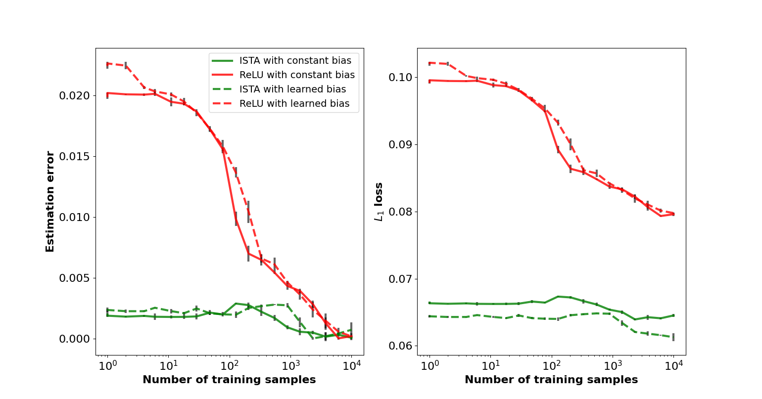
Figure 4: Comparing the EE of ISTA and ReLU networks with $2$ layers.

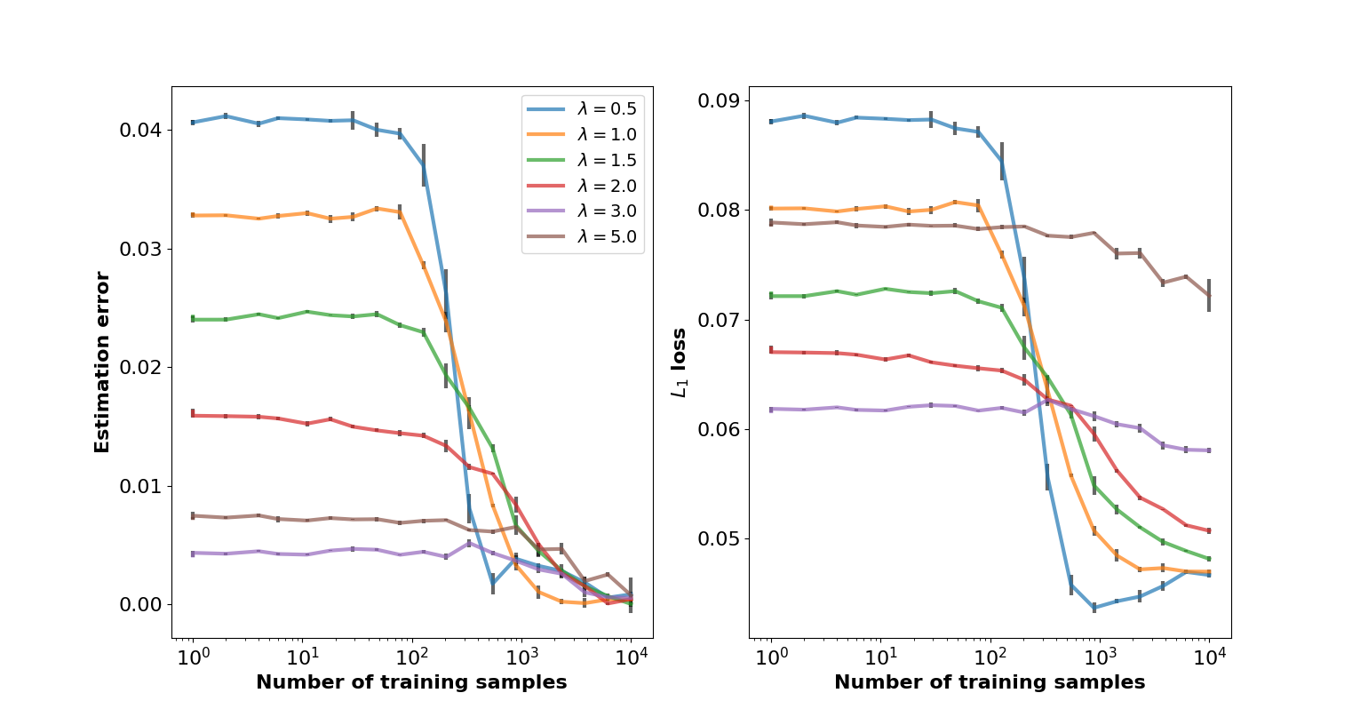
Figure 5: Estimation error and loss of ISTA networks with $2$ layers, as a function of the soft-threshold’s value $\lambda$.

Figure 6: Comparing the EE of ISTA and ReLU networks with $4$ layers.

Figure 7: Estimation error and loss of ISTA networks with $4$ layers, as a function of the soft-threshold’s value $\lambda$.

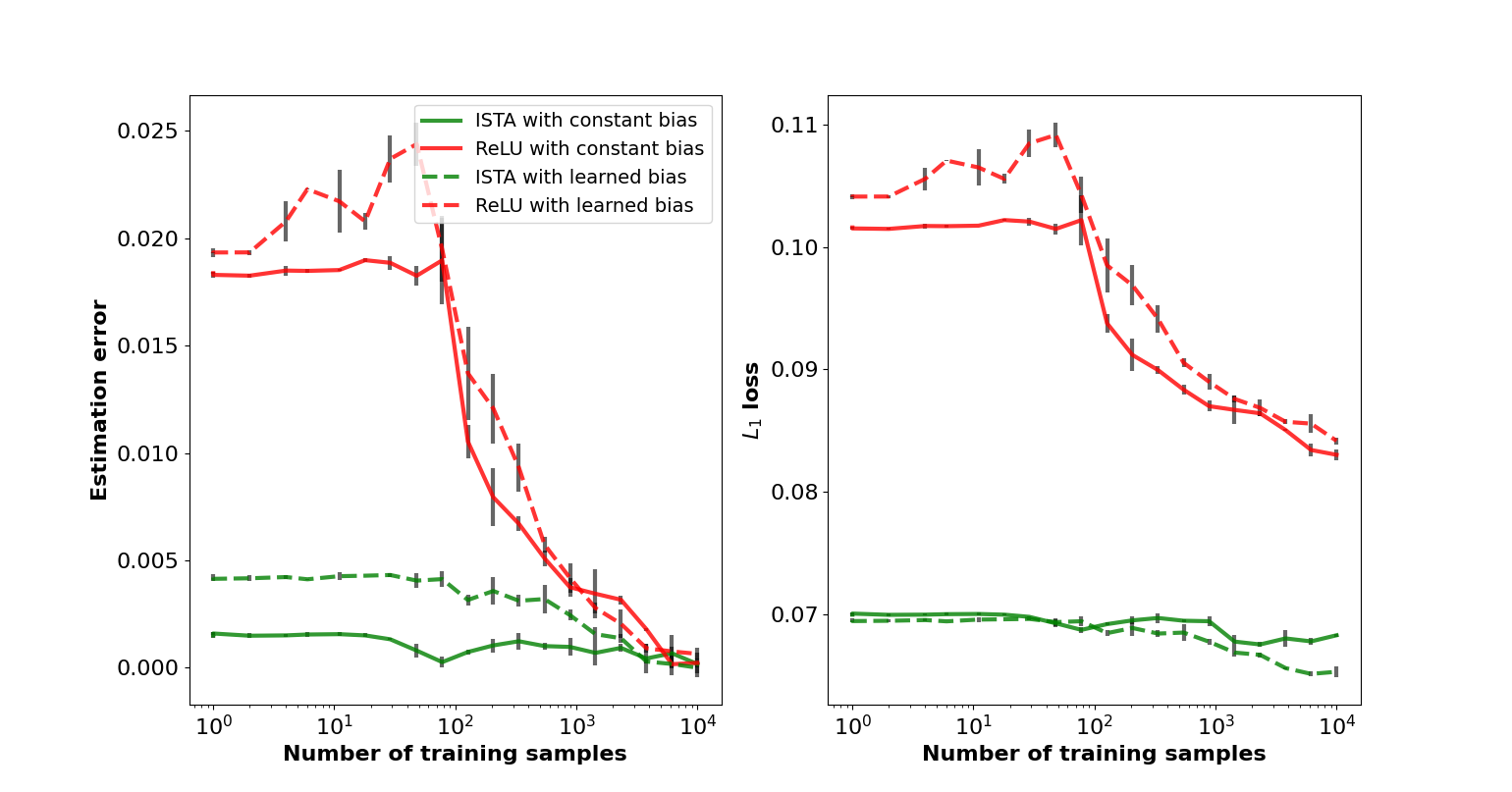
Figure 8: Comparing the EE of ISTA and ReLU networks with $6$ layers.

Figure 9: Estimation error and loss of ISTA networks with $6$ layers, as a function of the soft-threshold’s value $\lambda$.

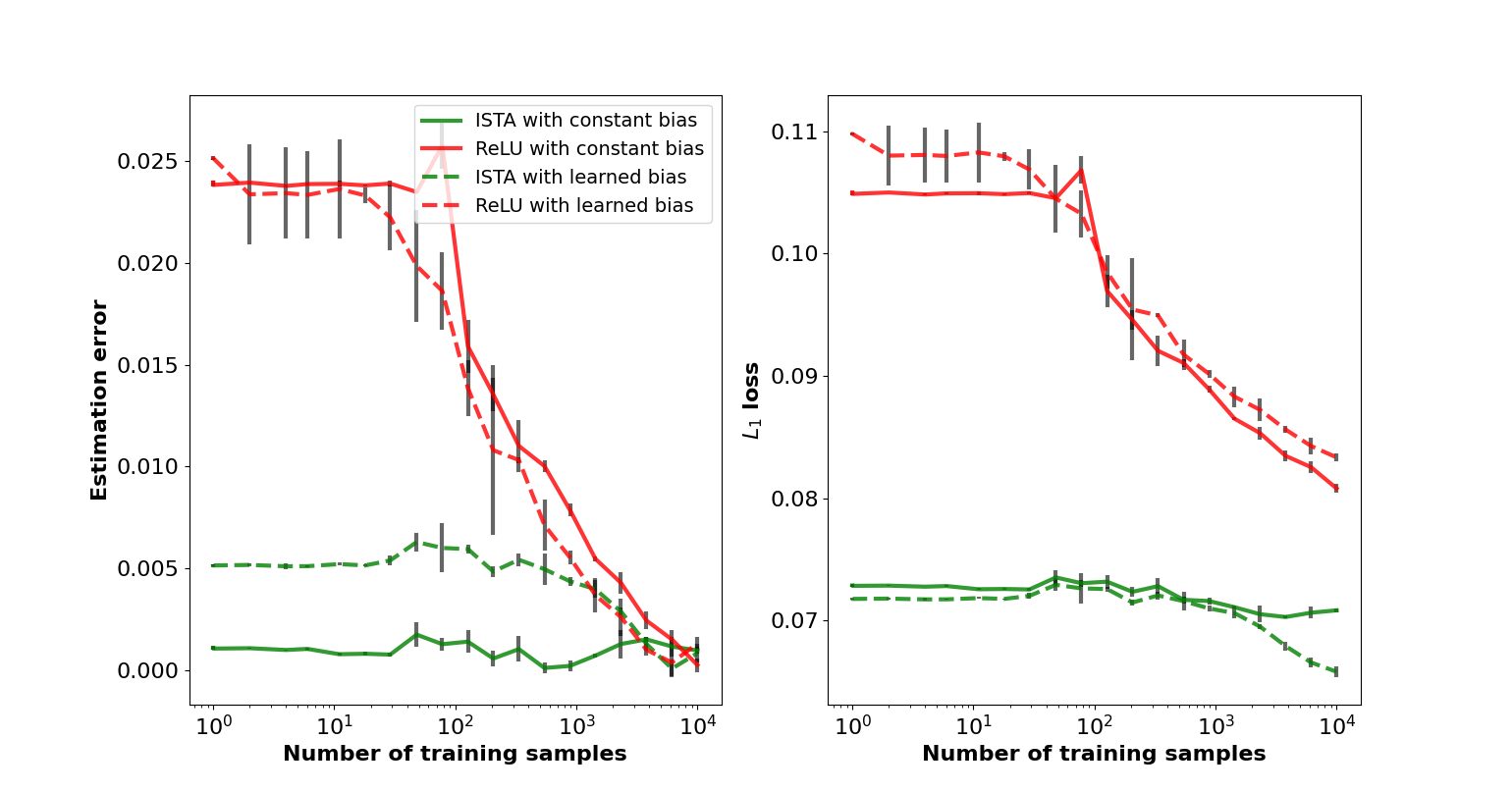
Figure 10: Comparing the EE of ISTA and ReLU networks with $8$ layers.

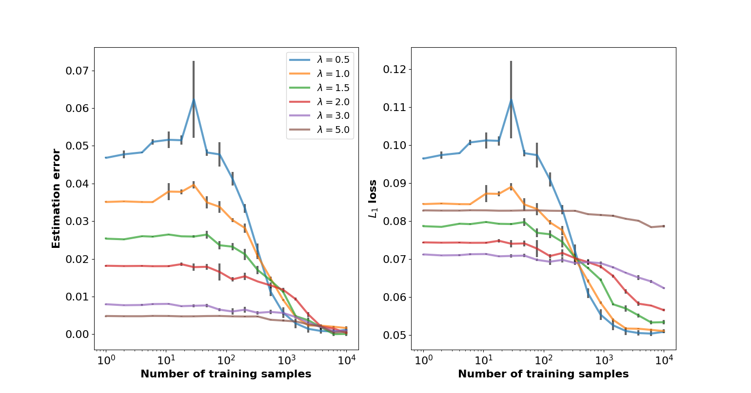
Figure 11: Estimation error and loss of ISTA networks with $8$ layers, as a function of the soft-threshold’s value $\lambda$.

References

- Amjad et al. (2021) J. Amjad, Z. Lyu, and M.R. Rodrigues. Deep learning model-aware regulatization with applications to inverse problems. IEEE Transactions on Signal Processing, 69:6371–6385, 2021.
- Authors (2022) Anonymous Authors. Model-based neural networks for sparse vector recovery. https://github.com/NeurIPS2022-Model-based-NN/Model_based_Network_Sparse_vector_recovery, 2022.
- Bartlett & Mendelson (2002) P.L. Bartlett and S. Mendelson. Rademacher and gaussian complexities: Risk bounds and structural results. Journal of Machine Learning Research, 3(3):463–482, 2002.
- Bartlett et al. (2005) P.L. Bartlett, O. Bousquet, and S. Mendelson. Local rademacher complexities. The Annals of Statistics, 33(4):1497–1537, 2005.
- Bartlett et al. (2017) P.L. Bartlett, D.J. Foster, and M.J. Telgarsky. Spectrally-normalized margin bounds for neural networks. Advances in neural information processing systems, 30, 2017.
- Behboodi et al. (2020) A. Behboodi, H. Rauhut, and E. Schnoor. Compressive sensing and neural networks from a statistical learning perspective. arXiv preprint arXiv:2010.15658, 2020.
- Belkin et al. (2019) M Belkin, D. Hsu, S. Ma, and S. Mandal. Reconciling modern machine-learning practice and the classical bias–variance trade-off. Proceedings of the National Academy of Sciences, 116(32):15849–15854, 2019.
- Blanchard et al. (2007) G. Blanchard, O. Bousquet, and L. Zwald. Statistical properties of kernel principal component analysis. Machine Learning, 66(2):259–294, 2007.
- Boyd et al. (2011) S. Boyd, N. Parikh, E. Chu, B. Peleato, and J. Eckstein. Distributed optimization and statistical learning via the alternating direction method of multipliers. Found. Trends Mach. Learn., 3(1):1–122, 2011.
- Gao & Zhou (2016) W. Gao and Z.H. Zhou. Dropout rademacher complexity of deep neural networks. Science China Information Sciences, 59(7):1–12, 2016.
- Golowich et al. (2018) N. Golowich, A. Rakhlin, and O. Shamir. Size-independent sample complexity of neural networks. Conference on Learning Theory, pp. 297–299, 2018.
- Gregor & LeCun (2010) K. Gregor and Y. LeCun. Learning fast approximations of sparse coding. Int. Conf. Machine Learning, pp. 399–406, 2010.
- Jakubovitz et al. (2019) D. Jakubovitz, R. Giryes, and M.R. Rodrigues. Generalization error in deep learning. Compressed sensing and its applications, pp. 153–193, 2019.
- Ledoux & Talagrand (1991) M. Ledoux and M. Talagrand. Probability in Banach Spaces: isoperimetry and processes. Springer Science Business Media, 1991.
- Lee et al. (2018) J. Lee, J. Sohl-dickstein, R. Pennington, J. Novak, S. Schoenholz, and Y. Bahri. Deep neural networks as gaussian processes. International Conference on Learning Representations, 2018.
- Liang et al. (2019) T. Liang, T. Poggio, A. Rakhlin, and J. Stokes. Fisher-rao metric, geometry, and complexity of neural networks. The 22nd international conference on artificial intelligence and statistics, pp. 888–896, 2019.
- Mendelson (2002) S. Mendelson. Improving the sample complexity using global data. IEEE transactions on Information Theory, 48(7):1977–1991, 2002.
- Monga et al. (2021) V. Monga, Y. Li, and Y.C. Eldar. Algorithm unrolling: Interpretable, efficient deep learning for signal and image processing. IEEE Signal Processing Magazine, 38(2):18–44, 2021.
- Neyshabur et al. (2015a) B. Neyshabur, R. Tomioka, and N. Srebro. Norm-based capacity control in neural networks. Conference on Learning Theory, pp. 1376–1401, 2015a.
- Neyshabur et al. (2015b) B. Neyshabur, R. Tomioka, and N. Srebro. In search of the real inductive bias: On the role of implicit regularization in deep learning. International Conference on Learning Representations workshop track, 2015b.
- Neyshabur et al. (2018) B. Neyshabur, Z. Li, S. Bhojanapalli, Y. LeCun, and N. Srebro. Towards understanding the role of over-parametrization in generalization of neural networks. arXiv preprint arXiv:1805.12076, 2018.
- Novak et al. (2018) R. Novak, Y. Bahri, D.A. Abolafia, J. Pennington, and J. Sohl-Dickstein. Sensitivity and generalization in neural networks: an empirical study. International Conference on Learning Representations, 2018.
- Ong et al. (2019) F. Ong, R. Heckel, and K. Ramchandran. A fast and robust paradigm for fourier compressed sensing based on coded sampling. International Conference on Acoustics, Speech and Signal Processing (ICASSP), pp. 5117–5121, 2019.
- Palomar & Eldar (2010) D.P. Palomar and Y.C Eldar. Convex optimization in signal processing and communications. Cambridge university press, 2010.
- Schnoor et al. (2021) E. Schnoor, A. Behboodi, and H. Rauhut. Generalization error bounds for iterative recovery algorithms unfolded as neural networks. arXiv preprint arXiv:2112.04364, 2021.
- Shalev-Shwartz & Ben-David (2014) Shai Shalev-Shwartz and Shai Ben-David. Understanding Machine Learning: From Theory to Algorithms. Cambridge University Press, USA, 2014. ISBN 1107057132.
- Sokolić et al. (2017) J. Sokolić, R. Giryes, G. Sapiro, and M.R. Rodrigues. Robust large margin deep neural networks. IEEE Transactions on Signal Processing, 65(16):4265–4280, 2017.
- Srivastava et al. (2014) N. Srivastava, G.E. Hinton, A. Krizhevsky, I. Sutskever, and R. Salakhutdinov. Dropout: a simple way to prevent neural networks from overfitting. Journal of machine learning research, 15(1):1929–2958, 2014.
- Tibshirani & Ryan (2013) Tibshirani and J. Ryan. The lasso problem and uniqueness. Electronic Journal of Statistics, 7(1):1465–1490, 2013.
- Vapnik & Chervonenkis (1991) V.N. Vapnik and A. Chervonenkis. The necessary and sufficient conditions for consistency in the empirical risk minimization method. Pattern Recognition and Image Analysis, 1(3):260284, 1991.
- Xu et al. (2016) C. Xu, T. Liu, D. Tao, and C. Xu. Local rademacher complexity for multi-label learning. IEEE Transactions on Image Processing, 25(3):1495–1507, 2016.
- Yang et al. (2018) Y. Yang, J. Sun, H. Li, and Z. Xu. Admm-csnet: A deep learning approach for image compressive sensing. IEEE transactions on pattern analysis and machine intelligence, 42(3):521–538, 2018.
- Yang et al. (2019) Y. Yang, J. Yu, X. Li, J. Huan, and T.S. Huang. An empirical study on regularization of deep neural networks by local rademacher complexity. arXiv preprint arXiv:1902.00873, 2019.
- Yousefi et al. (2018) N. Yousefi, Y. Lei, M. Kloft, M. Mollaghasemi, and G.C. Anagnostopoulos. Local rademacher complexity-based learning guarantees for multi-task learning. The Journal of Machine Learning Research, 19(1):1385–1431, 2018.
- Zhang (2002) T. Zhang. Effective dimension and generalization of kernel learning. Advances in Neural Information Processing Systems, 15, 2002.