K-means Clustering Based Feature Consistency Alignment
for Label-free Model Evaluation

Abstract

The label-free model evaluation aims to predict the model performance on various test sets without relying on ground truths. The main challenge of this task is the absence of labels in the test data, unlike in classical supervised model evaluation. This paper presents our solutions for the 1st DataCV Challenge of the Visual Dataset Understanding workshop at CVPR 2023. Firstly, we propose a novel method called K-means Clustering Based Feature Consistency Alignment (KCFCA), which is tailored to handle the distribution shifts of various datasets. KCFCA utilizes the K-means algorithm to cluster labeled training sets and unlabeled test sets, and then aligns the cluster centers with feature consistency. Secondly, we develop a dynamic regression model to capture the relationship between the shifts in distribution and model accuracy. Thirdly, we design an algorithm to discover the outlier model factors, eliminate the outlier models, and combine the strengths of multiple autoeval models. On the DataCV Challenge leaderboard, our approach secured 2nd place with an RMSE of 6.8526. Our method significantly improved over the best baseline method by 36% (6.8526 vs. 10.7378). Furthermore, our method achieves a relatively more robust and optimal single model performance on the validation dataset.

1 Introduction

Label-free model evaluation task, also known as AutoEval [9], requires models to evaluate the performance of datasets autonomously without explicit labels or categories. The models must identify inherent patterns and structures within the data without relying on pre-defined labels. Unlike supervised model evaluation [7, 30, 32, 13, 23, 33], AutoEval does not require a vast amount of labeled data, as shown in Figure 1, saving time and expensive costs. Furthermore, it can reveal potential data patterns and relationships that may not be discovered by supervised evaluation. However, this task is challenging due to the lack of explicit labels. Additionally, a test set comprises numerous images, and each image has varied and rich visual content [7]. In the 1st DataCV Challenge of the Visual Dataset Understanding workshop held at CVPR 2023 [1], participants are required to design a model that can estimate the accuracy of a given model on test sets without ground truths.

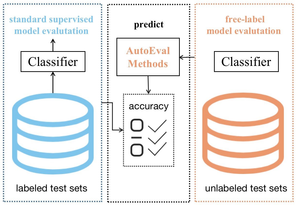
Figure 1: The illustration of label-free model evaluation. Given a classifier trained on the training set, we can obtain its performance by evaluating it on labeled test data set, as shown in (left). However, in label-free model evaluation scenarios, we encounter unlabeled test data sets, and cannot use common metrics to evaluate our classifiers (right).

In our daily lives, AutoEval mirrors real-world scenarios more closely. Evaluating the performance of an online model on out-of-time or out-of-distribution datasets typically requires data annotation, which can be prohibitively expensive and time-consuming. For instance, various risk data are often encountered in financial risk control scenarios. In order to detect various risky transactions, it is essential to evaluate the model’s performance in real-time. Hence, determining how to evaluate the model’s performance with unlabeled test datasets is crucial.

Recently, several studies have demonstrated promising performance in this task [16, 9, 8, 5, 26, 22, 14]. Calibration generated on the unseen distribution (target domain) yields consistent estimates and further helps infer the model’s performance [26, 14]. However, methods that require calibration in the target domain frequently produce poor estimates because deep learning models trained and calibrated on seen data (source domain) may not be calibrated in the previously unseen target domain. Some proposed methods [9, 8, 16] introduce additional labeled data from several target domains to learn a regression function of a distributional distance, which then predicts model performance. This method assumes that a strong correlation exists between the invisible test set and the visible train/val set in the fundamental distance measurement. The challenge baselines follow this paradigm, making it crucial to identify an appropriate linear correlation between the seen train sets and the unseen test sets and design an appropriate regression model. We address this challenge from three aspects: (1) designing excellent autoeval methods; (2) selecting the appropriate regressor; and (3) constructing the best integration strategy for multiple autoeval models.

To address the challenges stated above, we suggest three corresponding solutions. Firstly, we propose a novel model, K-means Clustering Based Feature Consistency Alignment (KCFCA), capable of representing the distribution shifts in various datasets. KCFCA utilizes the k-means clustering algorithm [17] to cluster the seen training set and unseen test set into clusters with a known number of categories. If the task at hand is N-classified, the centers of training samples and test samples that are clustered into N clusters should show close-to-distribution consistency. The distribution shifts between the two clustered centers can be used to fit a model regression. Secondly, experimental evidence has proved that different regression models will have a significant impact on the final result [9]. Therefore, we create a dynamic regression model that takes advantage of different regression models to fit the relationship between the shifts and the model accuracy. Thirdly, we design an outlier model factor discovery algorithm to eliminate outlier models and integrate the advantages of multiple autoeval models. In the course of this, we discover an interesting phenomenon: autoeval models based on various pre-trained models exhibit remarkable performance gaps. Lastly, our experiments validate the effectiveness of our solutions, and our model achieves second place on the DataCV Challenge leaderboard with an RMSE of 6.8526.

To summarize, this paper’s main contributions are as follows:

• We propose a novel method, K-means Clustering Based Feature Consistency Alignment (KCFCA), which can represent the distribution shifts in various datasets.

• We construct a dynamic regression model that fits the relationship between the distribution shifts and model accuracy.

• We design an outlier model factor discovery algorithm to eliminate outlier models and integrate the advantages of multiple autoeval models.

2 Related Work

Our work intersects with multiple related lines of research that have seen significant progress in recent years. Therefore, in this section, we provide a summary of the most closely related works.

2.1 Label-free Model Evaluation

Label-free model evaluation aims to predict the accuracy of an unseen test set when the ground truth is not accessible [16, 9, 8, 5, 26, 22, 14, 44]. This area has recently garnered widespread attention in the research community. Deng et al. [9] constructed a meta-dataset by transforming original images into various forms, adopted feature statistics to capture the distribution of a sample dataset, and trained a regression model to predict model performance. The difference of confidence was proposed [16] to yield successful estimates of a classifier’s performance across different shifts and model architectures. Such models rely on additional labeled data from several target domains to learn a linear regression function. The Average Thresholded Confidence (ATC) [14] method trained a threshold on the model’s confidence to predict accuracy as the fraction of unlabeled examples for which model confidence exceeds the threshold.

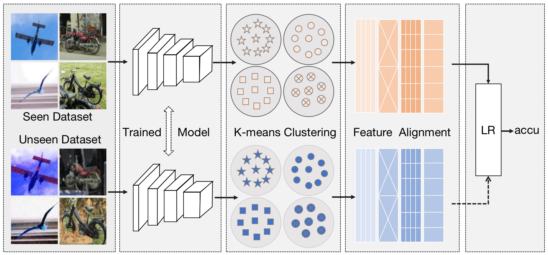
Figure 2: The illustration of Clustering Based Feature Consistency Alignment (KCFCA). KCFCA performs feature extraction by a pre-trained model, feature clustering with the K-means algorithm, feature alignment of the clustered features, and finally regression of feature shift using a regression model.

2.2 Out-Of-Distribution Detection

Out-of-distribution (OOD) detection is a critical task in machine learning that aims to identify examples outside the realm of the training distribution [36, 24, 21, 15, 28, 10, 39, 44, 31]. Model confidence outputs are commonly used as indicators to identify out-of-distribution samples [21, 15]. Liang et al. [28] proposed using temperature scaling and input perturbations to enhance OOD detection with model confidence. Devries and Taylor [10] introduced a method to learn confidence estimates for neural networks to produce intuitive and interpretable outputs. Sun et al. [41] designed ReAct - a straightforward and effective technique to reduce model overconfidence on OOD data, motivated by novel analysis on the internal activations of neural networks. Ren et al. [39] explored deep generative model-based approaches for OOD detection and observed that the likelihood score is heavily influenced by population-level background statistics. Learning the prediction uncertainty on OOD data remains a fundamental challenge in this task [36, 24].

2.3 Model Generalization Prediction

Predicting the generalization capabilities of models [2, 6, 25, 35, 43, 40, 4, 3] on unseen data has been a topic of interest in research for a long time. Complexity measurements on trained models and training sets have been explored as a means of predicting the generalization gap [2, 6, 25, 35]. Yang et al. [43] provided a simple explanation of this by measuring the bias and variance of neural networks to redefine how models generalize. Schiff et al. [40] used perturbation response (PR) curves to evaluate the accuracy change of a given network as a function of varying levels of training sample perturbation. Our work focuses on the cluster difference concerning the prediction of unseen test sets.

2.4 K-means Clustering

The k-means clustering algorithm is a popular unsupervised machine learning algorithm that serves to partition a given dataset into k clusters [17, 29, 37, 27, 34, 18]. In this algorithm, each data point is assigned to the cluster whose centroid is closest to it. The algorithm iteratively updates cluster centroids until convergence, which is achieved when the assignment of data points to clusters no longer changes. The basic principle of the k-means algorithm is to minimize the sum of squared distances between each data point and its assigned cluster centroid. The algorithm randomly initializes k centroids and then assigns each data point to the nearest centroid. In the next step, the centroids are updated by computing the mean of all the data points assigned to each cluster. This process is repeated until convergence. K-means is recognized as being both simple and efficient for partitioning datasets into k clusters. It has several advantages, such as computational efficiency and scalability.

3 Methods

3.1 Problem Formulation

We define this task by the source meta dataset $\mathcal{D}^{m}(\mathcal{D}_{train},\mathcal{D}_{val})$ (i.e. seen training dataset), which consists of the labeled training data $\mathcal{D}_{train}$ and validation data $\mathcal{D}_{val}$. Following the challenge and approach in [9], the source sample datasets $\mathcal{D}^{s}=\{\mathcal{D}_{i}(S_{xi},S_{yi})\}^{n}_{i=1}$ are transformed from the original $\mathcal{D}^{m}$, where $S_{xi}$ is the i-th training sample dataset, $S_{yi}$ are its corresponding labels, $n$ is the total number of the sample datasets, and $\mathcal{D}_{i}$ is the i-th sample dataset. In addition, the target unlabeled test set is denoted as $\mathcal{D}_{t}$, and does not contain any ground truths. We assume that the model $\mathcal{M}(\theta_{m})$ is pretrained on $\mathcal{D}^{m}$, where $\theta_{m}$ refers to the learned parameters that are fixed. If we have access to the label of $\mathcal{D}_{t}$, we can easily obtain the accuracy using $acc=\mathcal{M}(\mathcal{D}_{t}|\theta_{m})$. However, in the absence of labeled ground truth, the objective of this task is to predict the accuracy of the unlabeled test set under the a priori conditions of $\mathcal{D}^{m}$ and $\mathcal{M}(\theta_{m})$, which is expressed as Equation (1).

$$acc=f_{\theta}(\theta_{\omega},\mathcal{D}_{t}|(\mathcal{D}^{m},\mathcal{M}(\theta_{m})))$$ (1)

where $f_{\theta}(\cdot)$ represents the regression model that needs to be learned and $\theta_{\omega}$ are the parameters of this model.

Our work comprises three core components - K-means Clustering Based Feature Consistency Alignment (KCFCA), a novel AutoEval model that learns feature shifts between seen training data and unseen test data; Dynamic Regression Model (DRM), which strives to best fit the relationship between these shifts and model performance; and Outlier Model Factor Discovery (OMFD), which eliminates outlier autoeval models and integrates the advantages of multiple autoeval models. KCFCA will be discussed in Section 3.2, DRM in Section 3.3, and OMFD in Section 3.4.

3.2 K-means Clustering Based Feature Consistency Alignment

If we assume the meta task is a $\mathcal{N}$ classification task, then $\mathcal{M}(\theta_{m},X_{i})\in\{1,2,\cdots,\mathcal{N}\}$, where $X_{i}$ is i-th input image. By using the k-means clustering algorithm to cluster sample features, we can theoretically divide them into $\mathcal{N}$ clusters with the best silhouette coefficient [17]. Additionally, we propose K-means Clustering-based Feature Consistency Alignment, abbreviated as KCFCA and shown in Figure 2. We first review and summarize the K-means:

1. Initialize: Choose the number of clusters as K and select K random points (centroids) from the dataset as the initial centroids.

2. Assign: Assign each data point to the nearest centroid based on the euclidean distance between the data point and the centroids.

3. Update: Recalculate the centroids of each cluster by taking the mean of all the data points in that cluster.

4. Iterate: Repeat steps 2 and 3 until convergence, which occurs when the centroids no longer change or a maximum number of iterations is reached.

5. Output: The algorithm outputs the K clusters and K cluster centers, where each cluster contains a set of data points that are similar to each other and dissimilar to data points in other clusters.

As previously discussed, a dataset for a $\mathcal{N}$ classification task can be clustered into the most suitable $\mathcal{N}$ clusters. Given the sample datasets {$\mathcal{D}_{i}$, $\mathcal{D}_{train}$, $\mathcal{D}_{val}$}, and pretrained model $\mathcal{M}(\theta_{m})$, we construct dataset pairs as $\mathcal{D}_{sam}=\{\mathcal{D}_{sam_{i}}(\mathcal{D}_{i},\mathcal{D}_{val})\}^{n}_{i=1}$ that can calculate the accuracy $acc_{i}$. For each pair $\mathcal{D}_{sam_{i}}=(\mathcal{D}_{i},\mathcal{D}_{val})$, we first feed the $\mathcal{D}_{i}$ and $\mathcal{D}_{val}$ into the pretrained model $\mathcal{M}(\theta_{m})$ to extract the feature map $\mathcal{F}_{i}$ and $\mathcal{F}_{val}$. The feature $\mathcal{F}_{i}$ and $\mathcal{F}_{val}$ are then clustered into $\mathcal{N}$ clusters by K-means, with the cluster centers $\{\mathcal{F}_{ci}\}^{\mathcal{N}}_{ci=1}$ and $\{\mathcal{F}_{cval}\}^{\mathcal{N}}_{cval=1}$. Ideally, the distribution of each dataset pair should exhibit feature consistency. However, due to the uncertainty of unseen test data, distribution shifts often occur. Thus, we model the feature distance using frechet distance to fit these distribution shifts by [12, 9]. This distance is denoted as $D_{i}=D(\mathcal{F}_{ci},\mathcal{F}_{cval})$. Finally, a regression model $f_{\theta}(\cdot)$ is designed to regress the relations between $D_{i}$ and $acc_{i}$. KCFCA can be formulated as:

$$acc=f_{\theta}(\theta_{\omega},D(\mathcal{K}(\mathcal{M}(\theta_{m},\mathcal{D}_{val})),\mathcal{K}(\mathcal{M}(\theta_{m},\mathcal{D}_{i})))$$ (2)

where $\mathcal{K}(\cdot)$ is the k-means clustering algorithm.

The training and testing process of the model can be outlined as follows.

• Training: the regression model $f_{\theta}(\cdot)$ is adopted to learn the relation of $\{D_{i},acc_{i}\}$.

• Testing: calculate the feature distance between $\mathcal{D}_{val}$ and $\mathcal{D}_{t}$, put it into the regression model $f_{\theta}(\cdot)$, and obtain the dataset accuracy.

Specifically, the KCFCA algorithm can be represented as the following Algorithm 1.

Algorithm 1 K-means Clustering Based Feature Consistency Alignment

1:The sample datasets {$\mathcal{D}_{i}$, $\mathcal{D}_{train}$, $\mathcal{D}_{val}$}, and pretrained model $\mathcal{M}(\theta_{m})$

2:The accuracy of the unlabeled test set $\mathcal{D}_{t}$.

3:Training:

4:for number of source sample datasets training: do

5:     a. Feature extraction

6:         $\mathcal{F}_{i}=\mathcal{M}(\theta_{m},\mathcal{D}_{i}),\mathcal{F}_{val}=\mathcal{M}(\theta_{m},\mathcal{D}_{val})$

7:     b. K-means clustering

8:         $\{\mathcal{F}_{ci}\}^{\mathcal{N}}_{ci=1}=\mathcal{K}(\mathcal{F}_{i}),\{\mathcal{F}_{cval}\}^{\mathcal{N}}_{cval=1}=\mathcal{K}(\mathcal{F}_{val})$

9:     c. Feature distance

10:         $D_{i}=D(\mathcal{F}_{ci},\mathcal{F}_{cval})$

11:     d. Learn regression model

12:     $acc=f_{\theta}(\theta_{\omega},D(\mathcal{K}(\mathcal{M}(\theta_{m},\mathcal{D}_{val})),\mathcal{K}(\mathcal{M}(\theta_{m},\mathcal{D}_{i})))$

13:end for

14:

15:Testing:

16:Calculate the accuracy of $\mathcal{D}_{test}$:

17:$acc=f_{\theta}(\theta_{\omega},D(\mathcal{K}(\mathcal{M}(\theta_{m},\mathcal{D}_{val})),\mathcal{K}(\mathcal{M}(\theta_{m},\mathcal{D}_{t})))$

18:END

3.3 Dynamic Regression Model

In Section 1 and in our experiments of Section 4.2.2, we observed that different regression models have distinct advantages when using the same feature input. This highlights the importance of designing a suitable regression model. To address this issue, we propose a Dynamic Regression Model, named DRM, that incorporates the advantages of multiple regression models. DRM comprises several base regressors $f_{\theta_{b}}=\{f_{\theta_{bi}}\}_{i=1}^{m}$ and a meta-regressor $f_{\theta_{m}}$, where $m$ is the number of base regression models. As shown in Figure 3, the base regression models decouple to learn several sets of differentiated feature relations, while the meta-regression model dynamically fuses them to obtain a superior regression model. In other words, the meta-regressor learns base regression permutations of importance among the models. This procedure can be expressed as the following two equations:

$$f_{\theta_{m}}=\{\omega_{1},\omega_{2},\cdots,\omega_{m}\}$$ (3)

$$f_{\theta}=\omega_{1}\cdot f_{\theta_{b1}}+\omega_{2}\cdot f_{\theta_{b2}}+\cdots+\omega_{m}\cdot f_{\theta_{bm}}$$ (4)

where $\omega_{i}$ corresponds to the weight of the i-th base regressor.

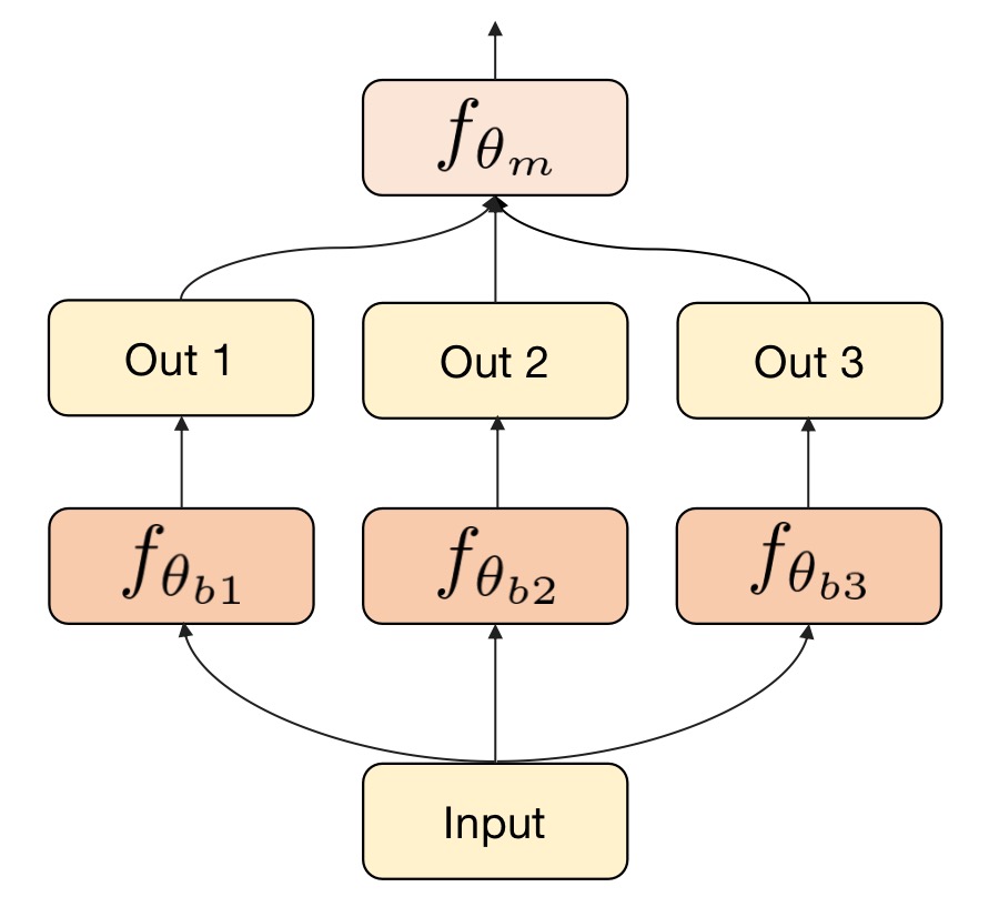
Figure 3: The illustration of proposed DRM. $f_{\theta_{bm}}$ means the base regression models, and $f_{\theta_{m}}$ is the meta regression model.

For the base regression models, the following algorithms can be utilized in the specific implementation: 1) Linear Regression. It works by finding the line of best fit that describes the relationship between the input variables (also known as features) and the output variable (also known as the target variable); 2) K-Nearest Neighbors Regressor. It works by finding the k closest data points to a given input data point in the feature space and then taking the average (or median) of the output variable of those k data points; 3) Support Vector Regression. It uses support vector machines (SVMs) to find the hyperplane that best separates the data into different classes. 4) Random Forest Regressor. It is an ensemble-based algorithm that builds multiple decision trees on random subsets of the data and input variables, and then averages the predictions of each tree to make the final prediction. As for the meta-regression model, we can easily adopt a fully connected network or vote regression.

3.4 Outlier Model Factor Discovery

As shown in Section 4.2.3, we observed that different autoeval algorithms have varying performance across distinct unlabeled test sets. In this challenge, combining different autoeval algorithms can improve the final prediction performance significantly. However, we found that simply fusing the results of all the algorithms cannot achieve optimal outcomes because outlier models may appear on different datasets or pre-trained models. Hence, we propose an Outlier Model Factor Discovery (OMFD) method to eliminate autoeval algorithms with lower performance stability.

Intuitively, most models predict that the consistency of results is more likely to be the correct result. Conversely, there is a possibility of the results being wrong. We denote the various performances of autoeval algorithms as $\mathcal{A}=\{\mathcal{A}_{i}\}_{i=1}^{m}$, where $\mathcal{A}_{i}$ is the i-th autoeval model. We define a threshold $\tau$ for the anomaly factor that measures whether the model is an anomalous outlier. The flow of OMFD can be illustrated as:

	Dataset A (RMSE $\downarrow$)				Dataset B (RMSE $\downarrow$)
Method	CIFAR-10.1	CIFAR-10.1-C	CIFAR-10-F	Overall	CIFAR-10.1	CIFAR-10.1-C	CIFAR-10-F	Overall
ConfScore [21]	2.190	9.743	2.676	6.985	1.584	9.897	2.63	7.074
Entropy [16]	2.424	10.300	2.913	7.402	1.849	10.537	2.949	7.561
Rotation [8]	7.285	6.386	7.763	7.129	–	–	–	–
ATC [14]	11.428	5.964	8.960	7.766	10.129	7.131	7.044	7.178
FID [9]	7.517	5.145	4.662	4.985	11.28	5.683	8.265	7.258
KCFCA (ours)	9.979	8.828	3.905	6.766	13.223	6.71	6.562	6.876

Table 1: The validation dataset results are based on the same pre-trained model. The colored cells are sub-optimal and optimal performance. “Dataset A” indicates the training dataset is provided by the challenge; “Dataset B” denotes the training dataset is regenerated using the same transformed strategy as the challenge and [9]. Note that we just generate such a training dataset in this part to validate the robustness of various autoeval methods, and we just use the training dataset provided by the challenge to summit in the challenge leaderboard.

1. Initialize: Visualize the performance of the autoeval model and manually select the appropriate centroid.

2. Calculate: Calculate the distance between the other autoeval models and this center.

3. Mark: If the maximum distance is greater than threshold $\tau$, the corresponding model is marked as an outlier.

4. Iterate: Repeat steps 1, 2 and 3 until convergence, which occurs when the maximum distance is no longer greater than the threshold $\tau$.

5. Output: Autoeval models marked as outliers.

We blend all the autoeval models except outlier models to achieve the best model performance. Note that the threshold $\tau$ can be debugged based on the validation set or set empirically.

4 Experiments

In all of our experiments, we follow the same dataset and settings as the DataCV Challenge [1].

4.1 Experimental Settings

4.1.1 Datasets

• Training dataset: The training dataset consists of 1,000 transformed datasets from the original CIFAR-10 test set, using the transformation strategy proposed by Deng et al. [9].

• Validation dataset: The validation set was composed of CIFAR-10.1 [38, 42], CIFAR-10.1-C [20] (add corruptions to CIFAR-10.1 dataset), and CIFAR-10-F (real-world images collected from Flicker.)

• Test dataset: The test set comprises 100 datasets provided by the challenge [1].

	ResNet-56 (RMSE $\downarrow$)						RepVGG-A0 (RMSE $\downarrow$)
Method	LR	KNN	SVR	MLP	RFR	DRM	LR	KNN	SVR	MLP	RFR	DRM
ConfScore [22]	6.985	7.708	7.559	12.028	7.765	7.503	8.721	8.998	9.647	16.603	9.098	8.841
Entropy [16]	7.401	7.510	8.033	18.284	7.695	7.546	9.093	9.398	9.647	9.647	9.566	9.277
Rotation [8]	7.129	7.723	7.502	13.207	8.209	7.603	13.391	11.144	10.130	18.651	11.303	11.172
ATC [14]	7.765	6.700	5.500	13.202	7.237	6.578	8.132	6.951	5.806	18.501	7.495	6.561
FID [9]	4.985	5.825	5.196	19.508	5.330	5.273	5.965	4.801	4.583	19.400	5.330	4.703

Table 2: Experimental results of different regression models on the same “Overall” validate datasets. “LR” is LinearRegression, “KNN” is the KNeighborsRegressor, “MLP” is the MLPRegressor, “RFR” is the RandomForestRegressor, and “DRM” is our dynamic regression model.

4.1.2 Pretrained classifier models

In our experiments, we follow this challenge and evaluate the classifiers ResNet-56 [19] and RepVGG-A0 [11]. Both implementations can be accessed in the public repository at the website. To benefit from the models and load their pre-trained weights, use the code provided on the website.

4.1.3 Evaluation metrics

The evaluation metric used in our experiments is the root-mean-square error (RMSE), which can be formulated as:

$$RMSE=\sqrt{\frac{\sum_{t=1}^{T}\left(\widehat{y}_{t}-y_{t}\right)^{2}}{T}}$$ (5)

4.2 Experiments and Findings

To verify the effectiveness of our proposed KCFCA, DRM, and OMFD, we conducted detailed experiments on the same validation datasets.

4.2.1 Experiments on various autoeval methods

In our study, we conduct comprehensive experiments on various autoeval methods, including ConfScore [21], Entropy [16], Rotation [8], ATC [14], FID [9], and our proposed KCFCA. All of the experiments are conducted based on the pre-trained ResNet56 provided by the challenge. Moreover, to validate the robustness of the various models, we perform experiments on 1,000 transformed datasets (denoted as “Dataset A”) provided by the challenge and an additional 1,000 transformed datasets (denoted as “Dataset B”) generated using the same transformation strategy as the challenge and [9]. Note that we only use the training dataset provided by the challenge to submit the challenge results.

Methods	Classifier	RMSE $\downarrow$	Classifier	RMSE $\downarrow$
ConfScore [22]	ResNet-56	6.985	RepVGG-A0	8.722
Entropy [16]	ResNet-56	7.402	RepVGG-A0	9.093
Rotation [8]	ResNet-56	7.129	RepVGG-A0	13.391
ATC [14]	ResNet-56	7.766	RepVGG-A0	8.132
FID [9]	ResNet-56	4.985	RepVGG-A0	5.966
AVG	ResNet-56	3.596	RepVGG-A0	4.244
OMFD (ours)	ResNet-56	2.873	RepVGG-A0	3.870

Table 3: The validation set results on mltiple autoeval methods. “Entries” indicates the number of submissions; $\downarrow$ means the smaller the value, the better.

The Table 1 provides us with some interesting conclusions. First, no single method can permanently lead on different validation sets, such as CIFAR-10.1, CIFAR-10.1-C, and CIFAR-10-F. This suggests that the unlabeled data have different domain shifts for diverse feature distributions. Second, overall, our proposed method KCFCA yields relatively robust results, including optimal performance on “Dataset B” and second-best performance on “Dataset A”.

4.2.2 Experiments on various regression methods

Our intuition tells us that choosing a variety of regressors will lead to different performance impacts. To investigate this, we perform an exhaustive experimental comparison of two pre-trained ResNet-56 and RepVGG-A0 models, using LinearRegression (LR), KNeighborsRegressor (KNN), SVR, MLPRegressor (MLP), RandomForestRegressor (RFR), our proposed Dynamic Regression Model (DRM) as regression models on ConfScore [21], Entropy [16], Rotation [8], ATC [14], and FID [9]. LR, KNN, SVR, MLP, and RFR are provided by Scikit-learn.

As shown in Table 2, it is rare to find a regression model that guarantees to outperform under all methods. However, it is evident that MLP has the least satisfactory outcome. It is encouraging to find that our proposed DRM can achieve relatively stable and excellent performance across different methods. For the final challenge submission, we experimentally use the LR regressor on ResNet-56 and the DRM regressor on RepVGG-A0.

4.2.3 Experiments on mltiple autoeval methods

To investigate the impact of different model fusion methods on the final challenge results, we conducted a series of experiments. The methods include ConfScore [21], Entropy [16], Rotation [8], ATC [14], FID [9], the average of all methods (AVG), and our proposed Outlier Model Factor Discovery (OMFD). We present all the results in Table 3.

The table indicates that averaging the results of all methods leads to decent results, surpassing any single method, with an average score of 3.870. However, leveraging our OMFD method to eliminate anomalous outlier methods leads to surprising optimal results of 2.873, a 34.7% improvement over the average score. Thus, our findings suggest that the inclusion of anomalous outlier methods is detrimental to the fusion process and adversely affects the final model output.

Teams	Classifier models	RMSE $\downarrow$
dlyldxwl	ResNet-56 & RepVGG-A0	6.3746
Yanglegeyang (ours)	ResNet-56 & RepVGG-A0	6.8526
SunshineBBB	ResNet-56 & RepVGG-A0	6.9438
Shiny	ResNet-56 & RepVGG-A0	8.6626
b136522541	ResNet-56 & RepVGG-A0	9.6994
xingjian	ResNet-56 & RepVGG-A0	10.7378

Table 4: The test set results on the DataCV Challenge leaderboard. “Entries” indicates the number of submissions; $\downarrow$ means the smaller the value, the better.

4.3 Results on DataCV Challenge

In the challenge, there are two models ResNet-56 and RepVGG- A0 is to be evaluated on the unlabeled test set in total by RMSE. The results of the challenge are shown in Table 4.

For our final challenge submission, we combined the K-means Clustering Based Feature Consistency Alignment (KCFCA), Dynamic Regression Model (DRM), and Outlier Model Factor Discovery (OMFD) methods. Our team secured second place in the challenge, as shown in the table. Additionally, our proposed approach outperformed the optimal model results [9] provided in the challenge, achieving a 36% improvement with a RMSE score of 6.8526 compared to 10.7378.

5 Conclusion

This paper highlights the various strategies we adopted in the challenge. Specifically, we propose the K-means Clustering Based Feature Consistency Alignment method to represent distribution shifts in different datasets, Dynamic Regression Model to analyze the relationship between shifts and model performance, and Outlier Model Factor Discovery to remove anomalous outlier autoeval models. Our approach secured second place in the challenge ranking. Furthermore, our KCFCA method achieved the most robust and optimal single model performance on the validation dataset.

References

- [1] The 1st datacv challenge @ cvpr 2023. In https://sites.google.com/view/vdu-cvpr23/competition.
- [2] Sanjeev Arora, Rong Ge, Behnam Neyshabur, and Yi Zhang. Stronger generalization bounds for deep nets via a compression approach. In International Conference on Machine Learning, pages 254–263. PMLR, 2018.
- [3] Jinghui Chen, Dongruo Zhou, Yiqi Tang, Ziyan Yang, Yuan Cao, and Quanquan Gu. Closing the generalization gap of adaptive gradient methods in training deep neural networks. arXiv preprint arXiv:1806.06763, 2018.
- [4] Lin Chen, Yifei Min, Mingrui Zhang, and Amin Karbasi. More data can expand the generalization gap between adversarially robust and standard models. In International Conference on Machine Learning, pages 1670–1680. PMLR, 2020.
- [5] Mayee Chen, Karan Goel, Nimit S Sohoni, Fait Poms, Kayvon Fatahalian, and Christopher Ré. Mandoline: Model evaluation under distribution shift. In International Conference on Machine Learning, pages 1617–1629. PMLR, 2021.
- [6] Ciprian A Corneanu, Sergio Escalera, and Aleix M Martinez. Computing the testing error without a testing set. In Proceedings of the IEEE/CVF Conference on Computer Vision and Pattern Recognition, pages 2677–2685, 2020.
- [7] Jia Deng, Wei Dong, Richard Socher, Li-Jia Li, Kai Li, and Li Fei-Fei. Imagenet: A large-scale hierarchical image database. In 2009 IEEE conference on computer vision and pattern recognition, pages 248–255. Ieee, 2009.
- [8] Weijian Deng, Stephen Gould, and Liang Zheng. What does rotation prediction tell us about classifier accuracy under varying testing environments? In International Conference on Machine Learning, pages 2579–2589. PMLR, 2021.
- [9] Weijian Deng and Liang Zheng. Are labels always necessary for classifier accuracy evaluation? In Proceedings of the IEEE/CVF Conference on Computer Vision and Pattern Recognition, pages 15069–15078, 2021.
- [10] Terrance DeVries and Graham W Taylor. Learning confidence for out-of-distribution detection in neural networks. arXiv preprint arXiv:1802.04865, 2018.
- [11] Xiaohan Ding, Xiangyu Zhang, Ningning Ma, Jungong Han, Guiguang Ding, and Jian Sun. Repvgg: Making vgg-style convnets great again. In Proceedings of the IEEE/CVF conference on computer vision and pattern recognition, pages 13733–13742, 2021.
- [12] DC Dowson and BV666017 Landau. The fréchet distance between multivariate normal distributions. Journal of multivariate analysis, 12(3):450–455, 1982.
- [13] M. Everingham, L. Van Gool, C. K. I. Williams, J. Winn, and A. Zisserman. The PASCAL Visual Object Classes Challenge 2012 (VOC2012) Results. http://www.pascal-network.org/challenges/VOC/voc2012/workshop/index.html.
- [14] Saurabh Garg, Sivaraman Balakrishnan, Zachary Chase Lipton, Behnam Neyshabur, and Hanie Sedghi. Leveraging unlabeled data to predict out-of-distribution performance. In International Conference on Learning Representations.
- [15] Yonatan Geifman and Ran El-Yaniv. Selective classification for deep neural networks. Advances in neural information processing systems, 30, 2017.
- [16] Devin Guillory, Vaishaal Shankar, Sayna Ebrahimi, Trevor Darrell, and Ludwig Schmidt. Predicting with confidence on unseen distributions. In Proceedings of the IEEE/CVF International Conference on Computer Vision, pages 1134–1144, 2021.
- [17] John A Hartigan and Manchek A Wong. Algorithm as 136: A k-means clustering algorithm. Journal of the royal statistical society. series c (applied statistics), 28(1):100–108, 1979.
- [18] John A Hartigan, Manchek A Wong, et al. A k-means clustering algorithm. Applied statistics, 28(1):100–108, 1979.
- [19] Kaiming He, Xiangyu Zhang, Shaoqing Ren, and Jian Sun. Deep residual learning for image recognition. In Proceedings of the IEEE conference on computer vision and pattern recognition, pages 770–778, 2016.
- [20] Dan Hendrycks and Thomas Dietterich. Benchmarking neural network robustness to common corruptions and perturbations. Proceedings of the International Conference on Learning Representations, 2019.
- [21] Dan Hendrycks and Kevin Gimpel. A baseline for detecting misclassified and out-of-distribution examples in neural networks. In International Conference on Learning Representations.
- [22] Dan Hendrycks and Kevin Gimpel. A baseline for detecting misclassified and out-of-distribution examples in neural networks. arXiv preprint arXiv:1610.02136, 2016.
- [23] Gao Huang, Zhuang Liu, and Kilian Q. Weinberger. Densely connected convolutional networks. CoRR, abs/1608.06993, 2016.
- [24] Xu Ji, Razvan Pascanu, R Devon Hjelm, Andrea Vedaldi, Balaji Lakshminarayanan, and Yoshua Bengio. Predicting unreliable predictions by shattering a neural network. 2021.
- [25] Yiding Jiang, Dilip Krishnan, Hossein Mobahi, and Samy Bengio. Predicting the generalization gap in deep networks with margin distributions. arXiv preprint arXiv:1810.00113, 2018.
- [26] Yiding Jiang, Vaishnavh Nagarajan, Christina Baek, and J Zico Kolter. Assessing generalization of sgd via disagreement. arXiv preprint arXiv:2106.13799, 2021.
- [27] Trupti M Kodinariya, Prashant R Makwana, et al. Review on determining number of cluster in k-means clustering. International Journal, 1(6):90–95, 2013.
- [28] Shiyu Liang, Yixuan Li, and Rayadurgam Srikant. Enhancing the reliability of out-of-distribution image detection in neural networks. arXiv preprint arXiv:1706.02690, 2017.
- [29] Aristidis Likas, Nikos Vlassis, and Jakob J Verbeek. The global k-means clustering algorithm. Pattern recognition, 36(2):451–461, 2003.
- [30] Tsung-Yi Lin, Michael Maire, Serge Belongie, James Hays, Pietro Perona, Deva Ramanan, Piotr Dollár, and C Lawrence Zitnick. Microsoft coco: Common objects in context. In Computer Vision–ECCV 2014: 13th European Conference, Zurich, Switzerland, September 6-12, 2014, Proceedings, Part V 13, pages 740–755. Springer, 2014.
- [31] Weitang Liu, Xiaoyun Wang, John Owens, and Yixuan Li. Energy-based out-of-distribution detection. Advances in neural information processing systems, 33:21464–21475, 2020.
- [32] Shuyu Miao, Shanshan Du, Rui Feng, Yuejie Zhang, Huayu Li, Tianbi Liu, Lin Zheng, and Weiguo Fan. Balanced single-shot object detection using cross-context attention-guided network. Pattern Recognition, 122:108258, 2022.
- [33] Shuyu Miao, Shuaicheng Li, Lin Zheng, Wei Yu, Jingjing Liu, Mingming Gong, and Rui Feng. Disentangled feature network for fine-grained recognition. In Neural Information Processing: 28th International Conference, ICONIP 2021, Sanur, Bali, Indonesia, December 8–12, 2021, Proceedings, Part II 28, pages 439–450. Springer, 2021.
- [34] Shi Na, Liu Xumin, and Guan Yong. Research on k-means clustering algorithm: An improved k-means clustering algorithm. In 2010 Third International Symposium on intelligent information technology and security informatics, pages 63–67. Ieee, 2010.
- [35] Behnam Neyshabur, Srinadh Bhojanapalli, David McAllester, and Nati Srebro. Exploring generalization in deep learning. Advances in neural information processing systems, 30, 2017.
- [36] Yaniv Ovadia, Emily Fertig, Jie Ren, Zachary Nado, David Sculley, Sebastian Nowozin, Joshua Dillon, Balaji Lakshminarayanan, and Jasper Snoek. Can you trust your model’s uncertainty? evaluating predictive uncertainty under dataset shift. Advances in neural information processing systems, 32, 2019.
- [37] Duc Truong Pham, Stefan S Dimov, and Chi D Nguyen. Selection of k in k-means clustering. Proceedings of the Institution of Mechanical Engineers, Part C: Journal of Mechanical Engineering Science, 219(1):103–119, 2005.
- [38] Benjamin Recht, Rebecca Roelofs, Ludwig Schmidt, and Vaishaal Shankar. Do cifar-10 classifiers generalize to cifar-10? 2018. https://arxiv.org/abs/1806.00451.
- [39] Jie Ren, Peter J Liu, Emily Fertig, Jasper Snoek, Ryan Poplin, Mark Depristo, Joshua Dillon, and Balaji Lakshminarayanan. Likelihood ratios for out-of-distribution detection. Advances in neural information processing systems, 32, 2019.
- [40] Yair Schiff, Brian Quanz, Payel Das, and Pin-Yu Chen. Predicting deep neural network generalization with perturbation response curves. Advances in Neural Information Processing Systems, 34:21176–21188, 2021.
- [41] Yiyou Sun, Chuan Guo, and Yixuan Li. React: Out-of-distribution detection with rectified activations. In M. Ranzato, A. Beygelzimer, Y. Dauphin, P.S. Liang, and J. Wortman Vaughan, editors, Advances in Neural Information Processing Systems, volume 34, pages 144–157. Curran Associates, Inc., 2021.
- [42] Antonio Torralba, Rob Fergus, and William T. Freeman. 80 million tiny images: A large data set for nonparametric object and scene recognition. IEEE Transactions on Pattern Analysis and Machine Intelligence, 30(11):1958–1970, 2008.
- [43] Zitong Yang, Yaodong Yu, Chong You, Jacob Steinhardt, and Yi Ma. Rethinking bias-variance trade-off for generalization of neural networks. In Hal Daumé III and Aarti Singh, editors, Proceedings of the 37th International Conference on Machine Learning, volume 119 of Proceedings of Machine Learning Research, pages 10767–10777. PMLR, 13–18 Jul 2020.
- [44] Yaodong Yu, Zitong Yang, Alexander Wei, Yi Ma, and Jacob Steinhardt. Predicting out-of-distribution error with the projection norm. In International Conference on Machine Learning, pages 25721–25746. PMLR, 2022.