The magnetic field and multiple planets of the young dwarf AU Mic

Abstract

In this paper we present an analysis of near-infrared spectropolarimetric and velocimetric data of the young M dwarf AU Mic, collected with SPIRou at the Canada-France-Hawaii telescope from 2019 to 2022, mostly within the SPIRou Legacy Survey. With these data, we study the large- and small-scale magnetic field of AU Mic, detected through the unpolarized and circularly-polarized Zeeman signatures of spectral lines. We find that both are modulated with the stellar rotation period (4.86 d), and evolve on a timescale of months under differential rotation and intrinsic variability. The small-scale field, estimated from the broadening of spectral lines, reaches $2.61\pm 0.05$ kG. The large-scale field, inferred with Zeeman-Doppler imaging from Least-Squares Deconvolved profiles of circularly-polarized and unpolarized spectral lines, is mostly poloidal and axisymmetric, with an average intensity of $550\pm 30$ G. We also find that surface differential rotation, as derived from the large-scale field, is $\simeq$30% weaker than that of the Sun. We detect the radial velocity (RV) signatures of transiting planets b and c, although dwarfed by activity, and put an upper limit on that of candidate planet d, putatively causing the transit-timing variations of b and c. We also report the detection of the RV signature of a new candidate planet (e) orbiting further out with a period of $33.39\pm 0.10$ d, i.e., near the 4:1 resonance with b. The RV signature of e is detected at 6.5$\sigma$ while those of b and c show up at $\simeq$4$\sigma$, yielding masses of $10.2^{+3.9}_{-2.7}$ and $14.2^{+4.8}_{-3.5}$ ${\rm M}_{\oplus}$ for b and c, and a minimum mass of $35.2^{+6.7}_{-5.4}$ ${\rm M}_{\oplus}$ for e.

1 Introduction

The formation of stars and their planets has become a very popular forefront topic of modern astrophysics, following the discovery of thousands of exoplanetary systems and the availability of many new powerful instruments capable of characterizing them, such as the JWST most recently. The goal of such studies is to investigate the surprising diversity of the exoplanetary systems detected around low-mass stars, and in particular to better understand the formation and evolution of planetary systems like ours. Studying newly born planetary systems and their pre-main-sequence (PMS) host stars is essential in this respect, the first evolutionary steps being those for which we currently have no more than weak observational constraints to guide theoretical models.

So far, very few multiple planetary systems younger than 50 Myr have been reported around low-mass stars, two of which detected with transit photometry, namely V1298 Tau (hosting 4 transiting planets, David et al., 2019) and AU Mic (with 2 known transiting warm Neptunes, Plavchan et al., 2020; Martioli et al., 2021; Szabó et al., 2021, 2022), then further monitored with precision Doppler velocimetry (Klein et al., 2021; Suárez Mascareño et al., 2021; Zicher et al., 2022). Given that young low-mass stars are usually quite active and strongly magnetic as a result of their short rotation periods (and convective envelopes), investigating their planets mandatorily requires characterization of the magnetic activity of the star so that the impact of this activity can be taken into account, and filtered out from the radial velocity (RV) curves in which planetary signatures hide. Constraining the large-scale magnetic fields of PMS stars is also essential for further documenting the parent dynamo processes that are able to amplify and sustain these fields, for investigating star-disc interactions and angular momentum evolution for stars whose accretion disc is still present (e.g., Zanni & Ferreira, 2013; Blinova et al., 2016), and for studying potential star-planet interactions that may occur if the planets orbit within the Alfven radius of their host stars (e.g., Strugarek et al., 2015). In this paper, we focus on the second and the brightest of these 2 stars, i.e., AU Mic.

AU Mic is an active M1 dwarf that belongs to the $\beta$ Pic moving group (aged $\simeq$20 Myr, Mamajek & Bell, 2014; Miret-Roig et al., 2020). Hosting an extended debris disc with moving features (Kalas et al., 2004; Boccaletti et al., 2015, 2018) and 2 known transiting warm Neptunes (Plavchan et al., 2020; Martioli et al., 2021), it is an ideal target for studying the formation and evolution of young planets and their atmospheres (Hirano et al., 2020). Several studies focused on estimating the masses of both planets, the 2 latest ones yielding $M_{b}=14.3\pm 7.7$ ${\rm M}_{\oplus}$ (where ${\rm M}_{\oplus}$ notes the Earth mass) and $M_{c}=34.9\pm 10.8$ (Klein et al., 2022), and $M_{b}=11.7\pm 5.0$ ${\rm M}_{\oplus}$ and $M_{c}=22.2\pm 6.7$ (Zicher et al., 2022). Given the large transit-timing variations (TTVs) of up to $\pm$10 min reported for planets b and c (Szabó et al., 2022), it is likely that the planetary system of AU Mic includes more, yet undetected, bodies. A new candidate Earth-mass planet (dubbed d), putatively located between b and c, was recently proposed to account for the reported TTVs (Wittrock et al., 2023). Besides, AU Mic is known for its intense activity and strong magnetic field (Kochukhov & Reiners, 2020; Klein et al., 2021), making it a prime target for studying dynamos of largely convective stars, magnetized winds and star-planet interactions (Kavanagh et al., 2021; Klein et al., 2022; Alvarado-Gómez et al., 2022), or escaping planetary atmospheres (Carolan et al., 2020).

In this paper, we report extended near-infrared (nIR) high-resolution spectropolarimetric observations of AU Mic with SPIRou at the 3.6-m Canada-France-Hawaii Telescope (CFHT) atop Maunakea in Hawaii, from early 2019 to mid 2022. After outlining our observations and data reduction in Sec. 2, we briefly revisit the main parameters of AU Mic in Sec. 3, compute the longitudinal and small-scale magnetic fields and their modulation with time in Sec. 4, carry out Zeeman-Doppler Imaging (ZDI) of our spectropolarimetric data at the main observing epochs in Sec. 5, study and model RV variations in Sec. 6, and investigate several activity proxies in Sec. 7. We finally summarize and discuss our results, and conclude by suggesting follow-up studies in Sec. 8.

2 SPIRou observations

AU Mic was intensively observed from early 2019 to mid 2022 with the SPIRou nIR spectropolarimeter / high-precision velocimeter (Donati et al., 2020) at CFHT, mostly within the SPIRou Legacy Survey (SLS), a Large Programme of 310 nights with SPIRou focussing on planetary systems around nearby M dwarfs on the one hand, and on the study of magnetized star / planet formation on the other. SPIRou collects spectra covering the entire 0.95–2.50 $\mu$m wavelength range in a single exposure, at a resolving power of 70,000, and for any given polarization state. A total of 235 circular polarization sequences on 194 different nights were collected on AU Mic with SPIRou over this 3-yr period, 181 in the framework of the SLS itself, 38 within the Director’s Discretionary Time PI program of Baptiste Klein (run ID 19AD97 and 19BD97, with results published in Klein et al., 2021), 15 within the PI program of Eric Gaidos (run ID 20AH93) and 1 within the PI program of Julien Morin (run ID 19AF26). As outlined in Donati et al. (2020), each SPIRou polarization sequence consists of 4 sub-exposures (except for one featuring 2 sub-exposures only due to bad weather). Each sub-exposure is associated with a different orientation of the Fresnel rhomb retarders (to remove systematics in polarization spectra to first order, see Donati et al., 1997), yielding one unpolarized (Stokes $I$) and one circularly polarized (Stokes $V$) spectrum. A series of 29 such spectra were also collected during the transit of AU Mic b on 2019 June 16, thanks to which Martioli et al. (2020) demonstrated, via the Rossiter-McLaughlin effect, that the planet orbit is prograde and lies in the equatorial plane of the host star (within 15^∘) and in the plane of the debris disk (Boccaletti et al., 2018).

With 10 of the 235 spectra collected in bad weather conditions and featuring much lower signal-to-noise ratio (SNR), we are left with a total of 225 Stokes $I$ and $V$ spectra of AU Mic collected on 188 different nights. Exposure times for most sequences are $\simeq$800 s, except for a few of them (e.g., those collected during the transit of AU Mic b) that were shorter (from 380 to 490 s). Peak SNRs range from 407 to 954 (median 785). The full log of our SPIRou observations is provided in Appendix A (see Table 5 provided as supplementary material) .

All data were processed with a new version of Libre ESpRIT, the nominal reduction pipeline of ESPaDOnS at CFHT, adapted for SPIRou (Donati et al., 2020). These reduced spectra were used in particular for the spectropolarimetric analyses outlined in Secs. 4 and 5. Least-Squares Deconvolution (LSD, Donati et al., 1997) was then applied to all reduced spectra, using a line mask constructed from the VALD-3 database (Ryabchikova et al., 2015) for an effective temperature $T_{\rm eff}$=3750 K and a logarithmic surface gravity $\log g$=4.5 adapted to young early M dwarfs like AU Mic (see Sec. 3), and selecting lines of relative depths larger than 3 percent only (for a total of $\simeq$1500 lines, featuring an average Landé factor of 1.2). The noise levels $\sigma_{V}$ in the resulting Stokes $V$ LSD profiles range from 0.73 to 1.73 (median 0.96) in units of $10^{-4}I_{c}$ where $I_{c}$ notes the continuum intensity. We also applied LSD to our spectra using 2 sub-masks of our main line mask, the high-Landé mask including lines with Landé factors larger than 1.5 (average Landé factor 1.7), and the low-Landé mask including lines with Landé factors lower than 1.0 (average Landé factor 0.7), both sub-masks featuring more or less the same number of lines ($\simeq$300) and the same average wavelength as the main mask ($\simeq$1700 nm).

In parallel, our data were also processed with APERO (version 0.7.275), the nominal SPIRou reduction pipeline (Cook et al., 2022), currently better optimised in terms of RV precision than Libre ESpRIT. The reduced spectra were then analysed by the line-by-line (LBL) technique (version 0.45, Artigau et al., 2022) to compute precise RVs for 185 of the 188 nightly-averaged observations collected on AU Mic, with a median RV error bar of 3.8 m s^-1 (see Table 5). Our RV data were also corrected for an overall trend, called Zero Point and coming from both the instrument and the reduction. It is inferred from a Gaussian Process Regression (GPR) applied to the RV curves of a dozen RV standard stars regularly monitored with SPIRou, and whose amplitude is small (RMS of a few m s^-1) with respect to the measured RV variations of AU Mic. Finally, in addition to RVs, the LBL analysis produces other diagnostics, in particular one measuring the variations in the average width of line profiles with respect to the median spectrum, which serves as an activity proxy (called differential line width or dLW in Artigau et al., 2022) linked to the Zeeman broadening of unpolarized spectra (see Sec. 4). These data were used for the RV analysis detailed in Sec. 6, and in the following section on activity proxies (Sec. 7).

3 Fundamental parameters of AU Mic

AU Mic (Gl 803, HD 197481, HIP 102409, $V=8.627$, $J=5.436$) is a bright M1 PMS dwarf located at a distance of $9.714\pm 0.002$ pc from us (Gaia Collaboration et al., 2021), with a rotation period of 4.86 d (Plavchan et al., 2020; Klein et al., 2021; Zicher et al., 2022), typical of its young age ($\simeq$20 Myr, Mamajek & Bell, 2014; Miret-Roig et al., 2020). As usual for young active M dwarfs, it exhibits photometric fluctuations caused by surface brightness inhomogeneities and flares, with an amplitude of a few percent (e.g., Plavchan et al., 2020; Martioli et al., 2021). Its mean $V-I$ color (equal to $2.034\pm 0.060$ mag, Kiraga, 2012) yields $\hbox{$T_{\rm eff}$}=3700\pm 70$ K (Pecaut & Mamajek, 2013), consistent with previous estimates (Gaidos et al., 2014; Malo et al., 2014; Afram & Berdyugina, 2019; Maldonado et al., 2020, quoting $3742\pm 83$, $3642\pm 22$, $3700-3800$ and $3755\pm 69$ K respectively). It implies that AU Mic has a bolometric magnitude of $7.22\pm 0.02$ mag and therefore a logarithmic luminosity with respect to the Sun $\log\hbox{$L_{\star}$}/\hbox{${\rm L}_{\odot}$}=-0.99\pm 0.01$, in agreement with, e.g., Malo et al. (2014) and Cifuentes et al. (2020). The inferred radius is $\hbox{$R_{\star}$}=0.78\pm 0.04$ ${\rm R}_{\odot}$.

The most recent interferometric measurements suggest a radius of $0.862\pm 0.052$ ${\rm R}_{\odot}$ (when taking into account limb darkening, Gallenne et al., 2022), slightly larger though still compatible with the previous value within 1$\sigma$. Given the rotation period of $4.86\pm 0.01$ d (the error bar indicating temporal variability rather than precision), these two $R_{\star}$ estimates translate into line-of-sight-projected rotation velocities at the equator of $\hbox{$v\sin i$}=8.1\pm 0.2$ and $9.0\pm 0.5$ km s^-1 respectively (AU Mic being seen almost equator on, Martioli et al., 2020; Martioli et al., 2021). From a fit to infrared spectral lines (including magnetic broadening), Kochukhov & Reiners (2020) find $\hbox{$v\sin i$}=9.2\pm 0.1$ km s^-1, consistent with the interferometric radius, although the authors mention that a smaller $v\sin i$ (of 8.1 km s^-1) is also possible when assuming a larger macroturbulence velocity (both being hard to determine independently). This further argues in favour of a radius in the range 0.80–0.85 ${\rm R}_{\odot}$ for AU Mic.

We used our spectra to redetermine the parameters of AU Mic with the tool designed for characterizing SPIRou spectra of M dwarfs (Cristofari et al., 2022a, b). Since magnetic fields significantly contribute to the width of spectral lines in stars as active and magnetic as AU Mic (López-Valdivia et al., 2021), we implemented polarized radiative transfer in the modeling (see Cristofari et al., 2023, and references therein for more information on the method) and carried out the analysis on the median SPIRou spectrum of AU Mic, including the effect of small-scale magnetic fields as in Kochukhov & Reiners (2020). In practice, we computed a grid of model spectra for different atmospheric parameters ($T_{\rm eff}$, $\log g$, metallicity ${\rm[M/H]}$, abundance of $\alpha$ elements relative to Fe $[\alpha/{\rm Fe}]$) and magnetic strengths (0, 2, 4, 6, 8 and 10 kG, assuming in each case a radial field of equal strength over the star), and ran a Monte Carlo Markov Chain (MCMC) process to find the atmospheric parameters and combination of magnetic spectra that best match the profiles of selected atomic and molecular lines with various magnetic sensitivities (including the Ti lines used by Kochukhov & Reiners 2020 and the field insensitive CO lines at 2.3 $\mu$m).

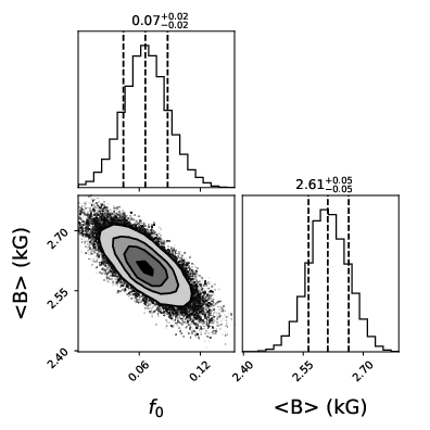
Figure 1: Magnetic parameters of AU Mic, derived by fitting our median SPIRou spectrum using the atmospheric modeling approach of Cristofari et al. (2023), which incorporates magnetic fields as well as a MCMC process to determine optimal parameters and their error bars. We find that AU Mic hosts a small-scale magnetic field of <$B$> $=2.61\pm 0.05$ kG, whereas the relative area of non-magnetic regions at the surface of the star is $f_{0}=0.07\pm 0.02$.

For the main atmospheric parameters, we find that $\hbox{$T_{\rm eff}$}=3665\pm 31$ K, $\hbox{$\log g$}=4.52\pm 0.05$, ${\rm[M/H]}=0.12\pm 0.10$ and $[\alpha/{\rm Fe}]=0.00\pm 0.04$. For the magnetic properties, we infer that the mean small-scale field at the surface of the star is <$B$> $=2.61\pm 0.05$ kG whereas the optimal coefficient associated with the non-magnetic spectrum $f_{0}$, i.e., the relative stellar surface area featuring no magnetic fields, is $f_{0}=0.07\pm 0.02$ (see Fig. 1). Most of the reconstructed field concentrates within the 2 and 4 kG bins (with respective filling factors $f_{2}=59$% and $f_{4}=33$%), whereas the 6, 8 and 10 kG bins ($f_{6}=1$%, $f_{8}=f_{10}=0$) can be ignored (Cristofari et al., 2023). We stress that taking magnetic fields into account is important to derive reliable atmospheric parameters of stars as magnetic as AU Mic, with potential overestimates, especially in $\log g$, when the effect of magnetic fields is neglected (Cristofari et al., 2023). The magnetic field at the times of our observations is stronger and covers a larger fraction of the star than at the time of the observations of Kochukhov & Reiners (2020).

Comparing the temperature and luminosity derived above (implying together a radius of $0.79\pm 0.02$ ${\rm R}_{\odot}$) with the evolutionary models of Siess et al. (2000, assuming solar metallicity and including overshoot) yields a mass of $\hbox{$M_{\star}$}=0.43\pm 0.03$ ${\rm M}_{\odot}$, a radius of $\hbox{$R_{\star}$}=0.74\pm 0.03$ ${\rm R}_{\odot}$ and an age of 13$\pm$2 Myr, which is lower than the age of the $\beta$ Pic moving group. Comparing now to the Baraffe et al. (2015) models gives a better agreement, with $\hbox{$M_{\star}$}=0.55\pm 0.05$ ${\rm M}_{\odot}$, $\hbox{$R_{\star}$}=0.78\pm 0.02$ ${\rm R}_{\odot}$ and an age of $17\pm 4$ Myr. Using the Dartmouth models (assuming again solar metallicity and including overshoot, Dotter et al., 2008) further improves the match with the measured parameters, yielding $\hbox{$M_{\star}$}=0.59\pm 0.04$ ${\rm M}_{\odot}$, $\hbox{$R_{\star}$}=0.79\pm 0.02$ ${\rm R}_{\odot}$ and an age of $20\pm 5$ Myr. All predicted radii are smaller than, though still reasonably close to, the interferometric one. In fact, active M dwarfs have repeatedly been reported to exhibit inflated radii with respect to theoretical models, possibly under the effect of magnetic fields (Chabrier et al., 2007; Morales et al., 2010; Feiden, 2016), although there is no consensus on this point yet (e.g., Morrell & Naylor, 2019).

We assume $\hbox{$M_{\star}$}=0.60\pm 0.04$ ${\rm M}_{\odot}$ and $\hbox{$R_{\star}$}=0.82\pm 0.02$ ${\rm R}_{\odot}$ for AU Mic in the rest of the paper, implying $\hbox{$v\sin i$}=8.5\pm 0.2$. The corresponding $\log g$ ($4.39\pm 0.05$) is slightly smaller that the one we measured, further arguing in favour of the Dartmouth models which yield a larger mass and thus a larger $\log g$ ($4.42\pm 0.05$) than the two others. Part of the discrepancy may also come from the fact that the standard atmospheric models we used to fit our SPIRou spectra may not be well adapted for young stars as strongly active and magnetic as AU Mic. We finally note that AU Mic is predicted to be still fully convective by the models of Siess et al. (2000), but to have already developed a small radiative core (of approximate mass and radius 0.2 $M_{\star}$ and 0.3 $R_{\star}$) in the models of Baraffe et al. (2015) and Dotter et al. (2008).

Parameters used in the following sections are listed in Table 1. Rotation cycles are computed using a rotation period of 4.86 d, and an arbitrary reference barycentric Julian date of BJD0 $=2459000$. (Note that a different BJD0 was used in Klein et al. 2021, causing phases in our study to be 0.394 rotation cycle larger for profiles common to both studies.)

Table 1: Parameters of AU Mic used in / derived from our study

distance (pc)	$9.714\pm 0.002$	Gaia Collaboration et al. (2021)
$V$ (mag)	$8.627\pm 0.052$	Kiraga (2012)
$V-I$ (mag)	$2.034\pm 0.060$	Kiraga (2012)
$J$ (mag)	$5.436\pm 0.017$	Cutri et al. (2003)
BCJ (mag)	$1.72\pm 0.01$	Pecaut & Mamajek (2013)
$\log(\hbox{$L_{\star}$}/\hbox{${\rm L}_{\odot}$})$	$-0.99\pm 0.01$	from $T_{\rm eff}$, $J$, BCJ and distance
$T_{\rm eff}$ (K)	$3665\pm 31$
$\log g$ (dex)	$4.52\pm 0.05$	$4.39\pm 0.05$ from mass and radius
${\rm[M/H]}$ (dex)	$0.12\pm 0.10$
$[\alpha/{\rm Fe}]$ (dex)	$0.00\pm 0.04$
$M_{\star}$ (${\rm M}_{\odot}$)	$0.60\pm 0.04$	using Dotter et al. (2008)
$R_{\star}$ (${\rm R}_{\odot}$)	$0.82\pm 0.02$
age (Myr)	$23\pm 3$	Mamajek & Bell (2014)
	$18.5\pm 2.4$	Miret-Roig et al. (2020)
$P_{\rm rot}$ (d)	$4.86$	period used to phase data
$P_{\rm rot}$ (d)	$4.856\pm 0.003$	period from $B_{\rm\ell}$ data
$P_{\rm rot}$ (d)	$4.866\pm 0.004$	period from RV data
$v\sin i$ (km s-1)	$8.5\pm 0.2$	from $P_{\rm rot}$ and $R_{\star}$
$i$	80∘	assumed for ZDI
	$89.5\pm 0.4$∘	orbit of b, Martioli et al. (2021)
<$B$> (kG)	$2.61\pm 0.05$
$f_{0}$	$0.07\pm 0.02$	$f_{2}=59$%, $f_{4}=33$%
$\Omega_{\rm eq}$ (rad d-1)	$1.299\pm 0.002$	average over 2020 and 2021
$d\Omega$ (mrad d-1)	$37\pm 7$	idem

4 The longitudinal field and Zeeman broadening of AU Mic

Using the Stokes $V$ and $I$ LSD profiles of AU Mic computed in Sec. 2, we computed the longitudinal field $B_{\rm\ell}$, i.e., the line-of-sight-projected component of the vector magnetic field averaged over the visible hemisphere, following Donati et al. (1997). The Stokes $V$ LSD signatures of AU Mic being quite broad, the first moment is computed over a domain of $\pm 45$ km s^-1 about the line center, whereas the equivalent width of the Stokes $I$ LSD profiles is simply estimated through a Gaussian fit (and found to be $\simeq$2 km s^-1). We also computed a null polarization check called $N$ (Donati et al., 1997), and derived a mean longitudinal field from this check, which is expected to be equal to 0 within the error bars and to yield a reduced chi-square $\chi^{2}_{\rm r}$ close to 1.

We thus obtained 225 $B_{\rm\ell}$ points over the full 3-yr timespan of our observations (see Table 5 for a complete log), as well as an equal number of values from the $N$ profiles. The corresponding $\chi^{2}_{\rm r}$ from $B_{\rm\ell}$ values and its equivalent from the $N$ profiles are respectively equal to 500 and 0.95 over the whole series, confirming that the field is detected and that the error bars are consistent with photon noise. We find that $B_{\rm\ell}$ ranges from -240 to 260 G, i.e., about an order of magnitude smaller than the average small-scale field <$B$> (see Sec. 3). We then carried out a quasi-periodic (QP) GPR fit to the $B_{\rm\ell}$ curve, with the covariance function $c(t,t^{\prime})$ set to

$$c(t,t^{\prime})=\theta_{1}^{2}\exp\left(-\frac{(t-t^{\prime})^{2}}{2\theta_{3}^{2}}-\frac{\sin^{2}\left(\frac{\pi(t-t^{\prime})}{\theta_{2}}\right)}{2\theta_{4}^{2}}\right)$$ (1)

where $\theta_{1}$ is the amplitude (in G) of the Gaussian Process (GP), $\theta_{2}$ its recurrence period (very close to $P_{\rm rot}$), $\theta_{3}$ the evolution timescale on which the $B_{\rm\ell}$ curve changes shape (in d), and $\theta_{4}$ a smoothing parameter setting the amount of allowed harmonic complexity. To these 4 hyper parameters, we added a fifth one called $\theta_{5}$ that describes the additional uncorrelated noise that is needed to obtain the QP GPR fit to the $B_{\rm\ell}$ data (denoted $y$) featuring the highest likelihood $\mathcal{L}$, defined by:

$$2\log\mathcal{L}=-n\log(2\pi)-\log|C+\Sigma+S|-y^{T}(C+\Sigma+S)^{-1}y$$ (2)

where $C$ is the covariance matrix for all observing epochs, $\Sigma$ the diagonal variance matrix associated with $y$, $S=\theta_{5}^{2}I$ the contribution of the additional white noise with $I$ the identity matrix, and $n$ the number of data points. Coupling this with a MCMC run to explore the parameter domain, we can determine the optimal set of hyper parameters and their posterior distributions / error bars.

The result of the fit is shown in Fig. 2 (top panel), with a zoom on seasons 2020 and 2021 also provided in the medium and bottom panels. The fitted GP parameters and error bars are listed in the top section of Table 2. All parameters are well defined, in particular the recurrence period $\theta_{2}$, found to be equal to $4.856\pm 0.003$ d (i.e., close to the estimates of Plavchan et al., 2020; Klein et al., 2021; Cale et al., 2021; Zicher et al., 2022) and the evolution timescale, which we measure at $80\pm 12$ d, i.e., half the duration of a typical observing season. The data are fitted to a RMS level of 6.2 G, slightly larger than the average error bar on our $B_{\rm\ell}$ measurements (of 5.2 G), yielding $\hbox{$\chi^{2}_{\rm r}$}=1.4$. The $B_{\rm\ell}$ data are thus not fitted down to the photon-noise level, suggesting an additional source of noise, e.g., intrinsic variability caused by activity (e.g., stochastic changes in the large-scale field, flares), modeled by the GP models with $\theta_{5}$ being significantly different from 0. The season-to-season variations of $B_{\rm\ell}$ are quite obvious, with the modulation shrinking to a minimum in October 2019 (BJD 2458800) and reaching a maximum in the following season (BJD 2459100). Moreover, as expected from the rather short evolution timescale, the fitted $B_{\rm\ell}$ curve also evolves significantly within each season, as can be seen on, e.g., the middle panel of Fig. 2. Running GPR on the 2020 and 2021 data subsets further suggests that evolution was faster in 2020 ($\theta_{3}=73\pm 11$ d) than in 2021 ($\theta_{3}=140\pm 40$ d).

Table 2: Results of our MCMC modeling of the $B_{\rm\ell}$ (first 5 rows) and <$B$> (last 5 rows) curves of AU Mic. For each hyper parameter, we list the fitted value along with the corresponding error bar, as well as the assumed prior. The knee of the modified Jeffreys prior is set to $\sigma_{B}$, i.e., the median error bars of our $B_{\rm\ell}$ and <$B$> estimates (i.e., 5.2 and 20 G respectively). For the recurrence period $\theta_{2}$, using a uniform prior yields the same result. For the evolution timescale $\theta_{3}$, the log Gaussian prior is set to 100 d (within a factor of 2), a typical value for early M dwarfs.

Parameter	Name	value	Prior
GP amplitude (G)	$\theta_{1}$	$100\pm 12$	mod Jeffreys ($\sigma_{B}$)
Rec. period (d)	$\theta_{2}$	$4.856\pm 0.003$	Gaussian (4.86, 0.1)
Evol. timescale (d)	$\theta_{3}$	$80\pm 12$	log Gaussian ($\log$ 100, $\log$ 2)
Smoothing	$\theta_{4}$	$0.43\pm 0.04$	Uniform (0, 3)
White noise (G)	$\theta_{5}$	$6.6\pm 0.9$	mod Jeffreys ($\sigma_{B}$)
GP amplitude (kG)	$\theta_{1}$	$0.16\pm 0.03$	mod Jeffreys ($\sigma_{B}$)
Rec. period (d)	$\theta_{2}$	$4.859\pm 0.004$	Gaussian (4.86, 0.1)
Evol. timescale (d)	$\theta_{3}$	$153\pm 18$	log Gaussian ($\log$ 100, $\log$ 2)
Smoothing	$\theta_{4}$	$0.71\pm 0.10$	Uniform (0, 3)
White noise (kG)	$\theta_{5}$	$0.01\pm 0.01$	mod Jeffreys ($\sigma_{B}$)

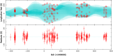
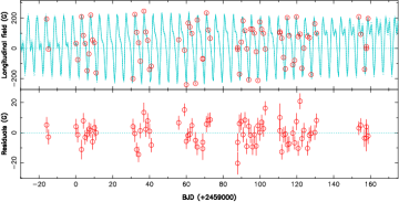
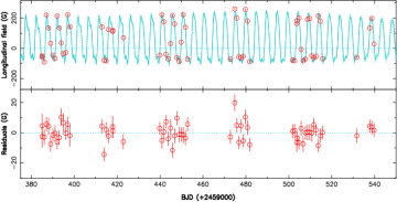
Figure 2: Longitudinal magnetic field $B_{\rm\ell}$ of AU Mic (red dots) over our observing period, and QP GPR fit to the data (cyan). The residuals are shown in the bottom plot of each panel. The top panel show the whole data set, whereas the lower 2 panels present a zoom on the 2020 and 2021 data respectively. The RMS of the residuals is 6.2 G, slightly larger than the average error bar of 5.2 G, yielding $\hbox{$\chi^{2}_{\rm r}$}=1.4$, whereas the $\chi^{2}_{\rm r}$ with respect to the weighted average is 442.

In parallel to the $B_{\rm\ell}$ analysis, we used the new tool of Cristofari et al. (2023), with which we analysed the nightly medians of our Stokes $I$ spectra (see Sec. 3), to derive the small-scale field at the stellar surface at each observing epoch and investigate its rotational modulation (freezing all non-magnetic parameters to the values derived from the median spectrum, even though magnetic and non magnetic parameters are mostly uncorrelated). The derived values of <$B$> are listed in Table 5. As for $B_{\rm\ell}$, we carried out a QP GPR on the <$B$> values, resulting in a $\chi^{2}_{\rm r}$ of 0.17, i.e., much lower than 1. It reflects that the retrieved formal error bars are absolute error bars (including systematics) rather than relative ones, thereby underestimating the precision at which night-to-night variations are measured. To derive relative error bars, we simply rescaled the formal ones using the dispersion of the residuals, thereby ensuring that the $\chi^{2}_{\rm r}$ of the QP GPR is close to 1 while $\theta_{5}$ remains consistent with 0. We obtained the results shown in Fig. 3 and the hyper-parameters listed in the bottom section of Table 2, yielding now $\hbox{$\chi^{2}_{\rm r}$}=0.78$.

We find that <$B$> is clearly modulated by the rotation cycle, with a recurrence period of $4.859\pm 0.004$ d, i.e., marginally larger than the one derived from $B_{\rm\ell}$. The semi-amplitude of the modulation is small, less than 0.1 kG in 2020 and reaching a maximum of 0.25 kG in 2022. We note that the modulation of <$B$> is smallest when that of $B_{\rm\ell}$ is largest and vice versa on our 4 observing seasons. Finally, the evolution timescale is twice longer for <$B$> than for $B_{\rm\ell}$. Over our 4 seasons of observations, <$B$> decreases from about 2.80 kG down to about 2.65 kG (see Fig. 3) and is on average slightly larger than that estimated from the median spectrum (see Sec. 3). More specifically, this weakening shows up as a decrease of the fitted 4 kG coefficient $f_{4}$, and a corresponding increase of the 2 kG coefficient $f_{2}$ (both being strongly anti-correlated, with a correlation coefficient $R=-0.90$). Whereas $f_{4}$ correlates with <$B$> ($R=0.70$) and varies from 0.32 to 0.18, $f_{2}$ is anti-correlated with <$B$> ($R=-0.80$) and varies from 0.60 to 0.75. We also note that, as for $B_{\rm\ell}$, the evolution of <$B$> as derived by GPR is faster in 2020 ($\theta_{3}=90\pm 30$ d) than in 2021 ($\theta_{3}=300\pm 100$ d). These results illustrate that both $B_{\rm\ell}$ and <$B$>, probing different characteristics of the field, are quite useful and very complementary to analyse the magnetic properties of active stars like AU Mic.

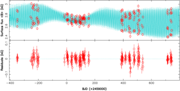
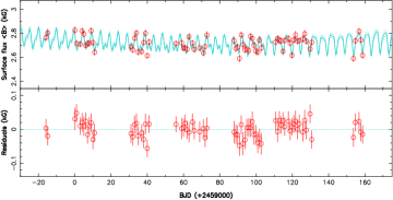
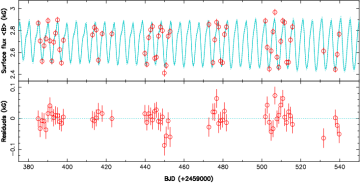
Figure 3: Same as Fig. 2 for the small-scale magnetic flux <$B$> at the surface of AU Mic. The RMS of the residuals is 0.02 kG, yielding $\hbox{$\chi^{2}_{\rm r}$}=0.78$, whereas the $\chi^{2}_{\rm r}$ with respect to the weighted average is 22.4.

We also looked at the Stokes $I$ LSD profiles computed with the high-Landé and the low-Landé masks. We find that the profiles from the first set are clearly broader than those from the second set as a result of Zeeman broadening, with the median full-width-at-half-maximum (FWHM) of the high-Landé and low-Landé LSD profiles being respectively equal to 31.9 and 22.5 km s^-1. The amount of quadratic differential broadening between the 2 sets of profiles is found to be $22.6\pm 1.0$ km s^-1 on average, with no clear evolution with time nor modulation with rotation phase. The FWHM of the high-Landé LSD profiles, dominated by Zeeman broadening, is weakly modulated by the rotation period and exhibits long-term variations of up to 2 km s^-1 over the full observing period. A GPR fit to the data yields a period of $4.85\pm 0.02$ d and a semi-amplitude of up to 1 km s^-1. A similar behaviour of about half the amplitude is observed on the FWHM of low-Landé LSD profiles. The overall trends on the FWHM of the LSD profile from high-Landé lines mimic those on <$B$>, i.e., a small decrease over the 4 seasons and a minimum modulation amplitude in 2020. The correlation factor between FWHMs and <$B$> is found to be $R=0.60$, suggesting that FWHMs can be used as an alternate proxy for <$B$>, albeit with a loss of precision.

5 Magnetic field and differential rotation of AU Mic

Using time-series of Stokes $V$ and $I$ LSD profiles, one can model the large-scale magnetic field at the surface of AU Mic, along with constraints on the small-scale field. This is achieved with ZDI, a tomographic imaging tool that inverts phase-resolved sets of LSD profiles into maps of the large-scale vector field (e.g., Donati et al., 2006; Klein et al., 2021). In the particular case of AU Mic, Stokes $I$ LSD profiles are significantly broadened by magnetic fields and can be used to further constrain the magnetic map and give insights on the small-scale field.

5.1 Zeeman-Doppler Imaging

In practice, ZDI proceeds iteratively, starting from a null magnetic field and adding information as it explores the parameter space using conjugate gradient techniques. At each iteration, ZDI compares the synthetic Stokes profiles of the current magnetic image with observed ones, and loops until it reaches the requested level of agreement with the data (i.e., a given $\chi^{2}_{\rm r}$). As the problem is ill-posed and features an infinite number of solutions of variable complexity, we choose the simplest one, i.e., the solution with minimum information or maximum entropy that matches the data at the requested level (e.g., Skilling & Bryan, 1984). The surface of the star is decomposed into 3000 grid cells. Local Stokes $I$ and $V$ profiles in each grid cell are computed using Unno-Rachkovsky’s equation of the polarized radiative transfer equation in a plane-parallel Milne Eddington atmosphere (Landi degl’Innocenti & Landolfi, 2004), then integrated over the visible surface of the star at each observed rotation phase (assuming a linear center-to-limb darkening law for the continuum, with a coefficient of 0.3) to yield the synthetic profiles corresponding to the reconstructed image. The mean wavelength and Landé factor of our LSD profiles are 1700 nm and 1.2.

The magnetic field at the surface of the star is described through a spherical harmonics (SH) expansion, using the formalism of Donati et al. (2006) in which the poloidal and toroidal components of the vector field are expressed with 3 sets of complex SH coefficients, $\alpha_{\ell,m}$ and $\beta_{\ell,m}$ for the poloidal component, and $\gamma_{\ell,m}$ for the toroidal component, where $\ell$ and $m$ note the degree and order of the corresponding SH term in the expansion.

ZDI can also model brightness inhomogeneities at the surface of the star, simultaneously with large-scale magnetic fields. In the particular case of AU Mic, we find that the distortions, and especially the broadening, of the LSD Stokes $I$ profiles are dominated by magnetic effects, with only a small impact of surface brightness inhomogeneities (in agreement with the small amplitude of photometric variations, of order of a few percent). For instance, the Doppler width of the local profile $v_{\rm D}$ that is needed to reproduce the average Stokes $I$ profile of AU Mic with minimal Zeeman broadening is found to be $\hbox{$v_{\rm D}$}=5.3$ km s^-1 (assuming $\hbox{$v\sin i$}=8.5$ km s^-1, see Sec. 3), whereas this parameter is typically equal to $\hbox{$v_{\rm D}$}\simeq 3$ km s^-1 for weakly-active, slowly-rotating M dwarfs of similar spectral type. The large difference in FWHM between the average Stokes $I$ LSD profiles associated with high-Landé and low-Landé lines (see Sec. 4) further confirms that this excess broadening is mostly of magnetic origin. In practice, we find that the Stokes $I$ and $V$ profiles of AU Mic can be entirely explained by magnetic field variations at the surface of the star. Consistently reproducing the FWHMs of the Stokes $I$ LSD profiles associated with high-Landé and low-Landé lines for small-scale fields of about 2.5 kG (see Sec. 4 and Kochukhov & Reiners, 2020) requires setting $\hbox{$v_{\rm D}$}=3.5$ km s^-1, on the high side of what is observed for weakly-active M dwarfs.

Given this, we chose to carry-out 2 different sets of complementary magnetic reconstructions. We first focus on Stokes $V$ LSD profiles only and assume $\hbox{$v_{\rm D}$}=5.3$ km s^-1, i.e., the Doppler width of the local profile that enables to reproduce Stokes $I$ LSD profiles with minimal Zeeman broadening. We further assume that only a fraction $f_{V}$ of each grid cell (called filling factor of the large-scale field, equal for all cells) actually contributes to Stokes $V$ profiles, with a magnetic flux over the cells equal to $B_{V}$ (and thus a magnetic field within the magnetic portion of the cells equal to $B_{V}/f_{V}$). This approach, called ‘Stokes $V$ analysis’ below, allows one to model the large-scale field and its temporal evolution over the 3 yr of our observations. It is similar to the study of Klein et al. (2021) in this respect (regarding $v_{\rm D}$ and $f_{V}$ in particular), except for simultaneous brightness imaging that has very little impact on the reconstructed magnetic map and that we therefore left out of the process.

In a second step, we model both Stokes $V$ and Stokes $I$ LSD profiles, this time assuming $\hbox{$v_{\rm D}$}=3.5$ km s^-1, i.e., the value that yields the observed FWHMs of the Stokes $I$ LSD profiles of high-Landé et low-Landé lines when the Zeeman broadening of a $\simeq$2.5 kG small-scale field is taken into account. This approach, called ‘Stokes $I$ & $V$ analysis’ below, leads to a significantly stronger reconstructed field (than in the Stokes $V$ analysis), which should now be consistent with both the large-scale field constraints provided by Stokes $V$ profiles and the small-scale field ones coming from Stokes $I$ data. In this case, we further assume that a fraction $f_{I}$ of each grid cell (called filling factor of the small-scale field, again equal for all cells) hosts small-scale fields of strength $B_{V}/f_{V}$ (i.e., with a small-scale magnetic flux over the cell equal to $B_{I}=B_{V}f_{I}/f_{V}$). This simple model implies in particular that the small-scale field locally scales up with the large-scale field (with a scaling factor of $f_{I}/f_{V}$), which is likely no more than a rough approximation. That the small-scale field is modulated with rotation (see Sec. 4) actually suggests that it may indeed spatially correlate with the large-scale field to some degree. In practice, we carried out ZDI for various values of $f_{I}$ and $f_{V}$, and selected the pair that fits the data best. In both cases, we assumed $i=80\hbox{${}^{\circ}$}$ for the inclination of the rotation axis to the line of sight, i.e., slightly lower than the inclination of the orbital planes of planets b and c (see Table 1), to reduce mirroring effects of the imaging process between the upper and lower hemispheres.

Both methods have their own pros and cons. The Stokes $V$ analysis makes it possible to optimally fit the Stokes $V$ profiles, yielding the minimal large-scale field (and variations with time) required by the data, but is not able to account for the observed small-scale field. It is well adapted to investigate the temporal evolution of the large-scale field, either from season to season, or under the effect of surface differential rotation (DR) within a given season. The Stokes $I$ & $V$ analysis is better suited to study the small-scale field and presumably yields a more accurate estimate of the large-scale field as well, but is less optimal to monitor its temporal changes. We did not attempt to model low-level brightness inhomogeneities whose impact on the Stokes $I$ and $V$ profiles is quite small, nor to model changes in the Stokes $I$ profiles caused by magnetic fields with pseudo-brightness features inducing similar profile distortions (as done in Klein et al., 2021). We report the results of both approaches in Secs. 5.2 and 5.3.

2019

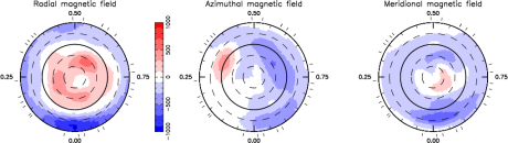
2020

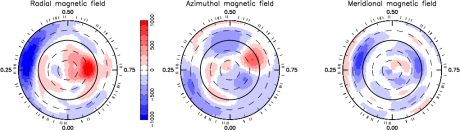
2021

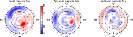
2022

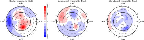
Figure 4: Reconstructed maps of the large-scale field of AU Mic (left, middle and right columns for the radial, azimuthal and meridional components in spherical coordinates, in G), for season 2019 Sep-Nov, 2020 Apr-Nov, 2021 Jun-Nov and 2022 May-Jun (top to bottom row respectively), derived from the Stokes $V$ LSD profiles of Fig. 13 using ZDI (see Sec. 5.2). The maps are shown in a flattened polar projection down to latitude $-60$^∘, with the north pole at the center and the equator depicted as a bold line. Outer ticks indicate phases of observations. Positive radial, azimuthal and meridional fields respectively point outwards, counterclockwise and polewards. Each image shows the evolving magnetic map (as a result of DR) at mid-time throughout the season.

Finally, we also looked for signatures of DR at the surface of the star, in the same way as in previous studies, i.e., by assuming a 2-parameter DR law similar to that of the Sun, with the rotation rate at latitude $\theta$ being given by $\Omega(\theta)=\hbox{$\Omega_{\rm eq}$}-\hbox{$d\Omega$}\sin^{2}\theta$, where $\Omega_{\rm eq}$ and $d\Omega$ respectively stand for the rotation rate at the equator and the difference in rotation rate between the equator and the pole. We then look for the pair of DR parameters that provides the best fit to the data at given image information content. To ensure maximum sensitivity, we concentrate on Stokes $V$ data only that are best suited for diagnosing temporal variability of the large-scale field. Results are reported in Sec. 5.4.

Since the timescale on which the large-scale field of AU Mic evolves ($\simeq$80 d, see Sec. 4) is much shorter than our overall observing window of 3 yr, we chose to divide our dataset into 4 different subsets, each more or less corresponding to one of our observing season (2019 Sep-Nov, 2020 Apr-Nov, 2021 Jun-Nov, 2022 May-Jun) containing respectively 28, 78, 65 and 20 spectra, and covering time slots of 57, 175, 155 and 33 d (about 12, 36, 32 and 7 rotation cycles), i.e., 0.4 to 2.2$\times$ the evolution timescale of the longitudinal magnetic field $\theta_{3}$ (80 d, see Sec. 4). The median time shifts between these 4 successive seasons, equal to 298, 391 and 265 d (about 61, 80 and 55 rotation cycles), are 3.3–4.9$\times$ larger than $\theta_{3}$. The few spectra collected early in 2019 April and June (at 6 main epochs, see Table 5), not providing enough phase coverage by themselves, were excluded from this analysis.

Images shown in Secs. 5.2 and 5.3 are derived with DR parameters of $\hbox{$\Omega_{\rm eq}$}=1.299$ rad d^-1 and $\hbox{$d\Omega$}=0.037$ rad d^-1, an average of the values we infer from our 2020 and 2021 data sets (see Sec. 5.4).

5.2 Stokes $V$ analysis of LSD profiles

The sets of Stokes $V$ LSD profiles collected with SPIRou for the 4 main seasons outlined previously, along with the ZDI fit to the data (assuming $\hbox{$v_{\rm D}$}=5.3$ km s^-1 for the Doppler width of the local profile), are presented in Fig. 13 (as supplementary material), whereas the corresponding reconstructed images are shown in Fig. 4. As in Klein et al. (2021), we find that $f_{V}\simeq 0.2$ provides the best fit to the data for all epochs. Error bars of Stokes $V$ LSD profiles (see Table 5) had to be increased by 40–60 percent for ZDI to be able to reach a unit $\chi^{2}_{\rm r}$, as with $B_{\rm\ell}$ for which GPR also diagnosed the presence of additional uncorrelated noise (see Sec. 4). The required increase in error bars is larger for our 2 longest seasons (2020 and 2021) and smaller for the shortest ones (2019 and 2022), further confirming that it likely reflects intrinsic variability from the intense activity of AU Mic.

Taking into account the phase shift mentioned in Sec. 3, our 2019 magnetic image resembles that of Klein et al. (2021), with a radial magnetic field reaching 700 G at phase 0.6 (phase 0.2 in Klein et al., 2021) at mid latitudes, along with consistent patches of azimuthal field of different polarities. Although both studies use the same data (except for one low-SNR observation, marked with an ’x’ in Table 5, left out from the first analysis and whose impact on the reconstructed image is insignificant), the two images are not exactly identical, the new one being reconstructed for a slightly larger $v\sin i$ (8.5 km s^-1 instead of 7.8 km s^-1) and a different pair of DR parameters (see Sec. 5.4). As a result, the field we reconstruct is slightly smaller than (though still consistent with) that of Klein et al. (2021), with a quadratically-averaged large-scale magnetic flux over the stellar surface equal to <$B_{V}$>$\simeq$380 G. The large-scale field is mostly poloidal and axisymmetric, with the poloidal component enclosing 75% of the reconstructed field energy, 75% of which in axisymmetric modes. The dipole component reaches a strength of $\hbox{$B_{\rm d}$}=430$ G at the pole, and is inclined at 15^∘ to the rotation axis towards phase 0.65.

2020

Figure 5: Same as second top row of Fig. 4 (2020 Apr-Nov), with the field now reconstructed using both Stokes $I$ & $V$ LSD profiles (see Sec. 5.3). Note the different color scale to depict magnetic fluxes.

The 2020 and 2021 images are reconstructed from data sets covering a 3$\times$ longer time span and are thus much better constrained, especially regarding DR (see Sec. 5.4). Again, we find that AU Mic hosts a dominantly poloidal large-scale field enclosing 85% of the reconstructed energy (of which 35% in axisymmetric modes), and that <$B_{V}$> ranges from 360 G (in 2021) to 400 G (in 2020). Both magnetic maps feature a strong positive radial field region at a latitude of 30^∘ (at phases 0.73 in 2020 and 0.91 in 2021) where $B_{V}$ reaches 1.2 kG, and another similar one of opposite polarity in the other hemisphere, located more or less symmetrically from the positive one with respect to the centre of the star. These radial field regions are accompanied by an azimuthal field region of identical polarity, located at a similar latitude and a slightly smaller phase. Apart from a global phase shift (of 0.17 cycle) that likely reflects the effect of DR at a latitude of $\simeq$30^∘ over the time span that separates both data sets (equal to 80 rotation cycles of AU Mic), the 2020 and 2021 magnetic maps share obvious similarities, featuring dipole components of $\hbox{$B_{\rm d}$}=440$ G and 400 G respectively tilted at 40^∘ and 50^∘ to the rotation axis (towards phase 0.75 and 0.85). Despite this resemblance, the detailed maps depart enough from one another to generate $B_{\rm\ell}$ curves that are significantly different, as a result of temporal evolution (on a timescale of 80 d, see Sec. 4 and Fig. 2).

Although derived from the sparsest of our 4 data sets, the 2022 magnetic image of AU Mic is largely similar to the previous ones, with a 1 kG positive radial field region reconstructed at mid latitude (phase 0.96), but with the main negative radial field region no longer showing up at the antipodes of the positive one. The azimuthal field regions accompanying the radial field ones are also much weaker than in the previous 2 images. We find that <$B_{V}$>, equal to 330 G, is weaker than in the previous seasons, and so is the dipole component $\hbox{$B_{\rm d}$}=380$ G (tilted at 35^∘ towards phase 0.80). Once more, the poloidal component largely dominates the large-scale field topology, enclosing 90% of the reconstructed magnetic energy, 45% of which in axisymmetric modes.

All properties of the reconstructed large-scale magnetic field are summarised in Table 3 for our 4 observing seasons.

Table 3: Properties of the large-scale (columns 2 to 6 and 8 to 10) and small-scale (column 7) magnetic field of AU Mic for our 4 observing seasons. Columns 2 to 5 correspond to the ZDI Stokes $V$ analysis (assuming $f_{V}=0.2$ and $\hbox{$v_{\rm D}$}=5.3$ km s^-1, see Sec. 5.2), whereas columns 6 to 10 summarize the results of the ZDI Stokes $I$ & $V$ analysis (assuming $f_{I}=0.9$, $f_{V}=0.2$ and $\hbox{$v_{\rm D}$}=3.5$ km s^-1, see Sec. 5.3). Columns 3 and 8 list the polar strengths of the dipole component $B_{\rm d}$, columns 4 and 9 the tilts of the dipole component to the rotation axis, and columns 5 and 10 the amount of magnetic energy reconstructed in the poloidal component of the field and in the axisymmetric modes of this component. Error bars on field values and percentages are typically equal to 5–10%.

	Stokes $V$ analysis				Stokes $I$ & $V$ analysis
	($f_{V}=0.2$, $\hbox{$v_{\rm D}$}=5.3$ km s-1)				($f_{I}=0.9$, $f_{V}=0.2$, $\hbox{$v_{\rm D}$}=3.5$ km s-1)
Season	<$B_{V}$>	$B_{\rm d}$	tilt	poloidal / axisym	<$B_{V}$>	<$B_{I}$>	$B_{\rm d}$	tilt	poloidal / axisym
	(G)	(G)	(∘)	(%)	(G)	(kG)	(G)	(∘)	(%)
2019 Sep-Nov	380	430	15	75 / 75	550	2.5	650	10	85 / 90
2020 Apr-Nov	400	440	40	85 / 35	570	2.6	660	25	90 / 75
2021 Jun-Nov	360	400	50	85 / 35	530	2.4	650	25	90 / 75
2022 May-Jun	330	380	35	90 / 45	520	2.3	660	20	90 / 80

5.3 Stokes $I$ & $V$ analysis of LSD profiles

We now analyse Stokes $I$ and $V$ LSD profiles together, setting now $\hbox{$v_{\rm D}$}=3.5$ km s^-1 for the Doppler width of the local profile. It allows us to infer constraints on the small-scale and large-scale magnetic fields $B_{I}$ and $B_{V}$ simultaneously, under the assumption that the first scales up with the second with a fixed factor of $f_{I}/f_{V}$ (see Sec. 5.1). In practice, we find that $f_{I}=0.9$ provides good results, in rough agreement with the results of Sec. 3, implying a scaling factor of the small-scale to large-scale field equal to $f_{I}/f_{V}=4.5$. This is also consistent with previous results, indicating that active M dwarfs like AU Mic are able to trigger large-scale fields <$B_{V}$> whose strength reaches up to 30 percent that of small-scale fields <$B_{I}$> (Morin et al., 2010; Kochukhov, 2021).

With this approach, we find that the large-scale field of AU Mic is significantly stronger than that derived in Sec. 5.2, including in particular a more intense, mostly axisymmetric, dipole component. This is consistent with the small-scale field <$B$> directly measured from magnetically sensitive lines, and from the observed differential broadening between the high-Landé and low-Landé Stokes $I$ LSD profiles. 4). Since small-scale fields are assumed to scale-up with large-scale fields in our simple model, ZDI has no other choice than increasing the large-scale field as well to generate the adequate level of magnetic broadening in the Stokes $I$ LSD profiles. Despite this additional constraint, ZDI is still able to fit the Stokes $V$ LSD profiles at the same time as the Stokes $I$ LSD profiles, adding to the large-scale field a nearly axisymmetric dipole component that contributes no more than marginally to the Stokes $V$ profiles (as a result of the geometrical configuration, with the star being close to equator-on for an Earth-based observer).

The properties of the reconstructed magnetic fields are summarized in columns 6 to 10 of Table 3 for our 4 seasons. In average, we find that <$B_{V}$> now reaches fluxes of 520–570 G, i.e., 1.5$\times$ larger than when fitting Stokes $V$ LSD profiles only. It implies small-scale field fluxes of <$B_{I}$>=2.3–2.6 kG, in agreement with the results of Secs. 3 and 4, as well as with those of Kochukhov & Reiners (2020). The difference with the results of Sec. 5.2 also shows up on the inferred dipole component, now 1.6$\times$ larger than in the Stokes $V$-only reconstruction, with the poloidal component enclosing 75–90% of the reconstructed magnetic energy. As the added dipole is mostly axisymmetric, the tilt of the overall dipole component to the rotation axis is smaller (10-25^∘) and the poloidal component is mostly axisymmetric (75–90% in terms of magnetic energy). We show one example reconstruction for season 2020 in Fig. 5, the inferred maps for the 3 other seasons looking similar.

We stress that, although our new set of magnetic maps are able to fit both Stokes $I$ and $V$ data, they may still not match the real ones as the imaging problem is ill-posed. This is especially true for AU Mic, whose almost equator-on orientation and small $v\sin i$ both contribute to the problem degeneracy. For instance, adding small-scale tangled fields more or less evenly at the surface of AU Mic without modifying the large-scale field reconstructed from Stokes $V$ profiles only, may also provide a comparable fit to the Stokes $I$ and $V$ profiles, but with a magnetic topology that does not have a fixed amount of small-scale to large-scale field ratio over the surface. This second model would however generate very little rotational modulation of the small-scale field, thereby contradicting our <$B$> measurements from magnetically sensitive lines (see Sec. 4). Further constraining the imaging process would require collecting LSD profiles for Stokes $Q$ and $U$ LSD profiles, in addition to Stokes $V$ and $I$ profiles, as previously suggested by Kochukhov & Reiners (2020). Fig. 14 (provided as supplementary material) shows for instance that Stokes $Q$ and $U$ signatures (not measured in our campaign) would be detectable and allow one to unambiguously differentiate between the maps of Secs. 5.2 and 5.3.

5.4 Differential rotation from Stokes $V$ LSD profiles

Last but not least, one can study the amount of latitudinal DR shearing the surface of AU Mic from the recurrence periods of the Stokes $V$ signatures associated with the magnetic features reconstructed at different latitudes. As the goal is to diagnose subtle evolution of the Stokes $V$ signatures with time, the most reliable approach is to focus on Stokes $V$ LSD profiles only (as in Sec. 5.2), even though the large-scale field itself may actually be stronger than what Stokes $V$ LSD profiles alone indicate (see Sec. 5.3). As outlined in Sec. 5.1, this is achieved by reconstructing magnetic maps at given information content (i.e., at given magnetic energy) over a given grid of DR parameters. We then fit the resulting $\chi^{2}_{\rm r}$ map with a 2D paraboloid, the location of the minimum and the paraboloid curvature at this location respectively providing the optimal DR parameters and the associated error bars (Donati et al., 2003).

We first find that data sets corresponding to seasons 2019 and 2022 do not span long enough a time slot and include too few profiles to yield reliable DR estimates, especially for a star like AU Mic whose $v\sin i$ is on the low side, and that exhibits a high level of intrinsic variability, even on its large-scale field (see Sec. 4). More specifically, we find that the derived $\chi^{2}$ maps for both epochs are noisy, showing low-level fluctuations with no obvious minimum over the grid of DR parameters, possibly as a result of short-term intrinsic variability distorting magnetic maps and preventing the DR signal to build-up in a consistent way. For season 2019 and with the same data, Klein et al. (2021) was able to locate a minimum in the $\chi^{2}_{\rm r}$ map outside our grid of DR parameters, corresponding to an unexpectedly strong DR for an M dwarf like AU Mic. We thus suspect this early estimate to rather reflect the impact of intrinsic variability rather than the shearing effect of DR.

   

Figure 6: Measuring DR at the surface of AU Mic by minimizing the $\chi^{2}_{\rm r}$ of the ZDI fit to our Stokes $V$ LSD profiles over a grid of DR parameters (see Sec. 5.4), for season 2020 Apr-Nov (left panel) and 2021 Jun-Nov (right panel). In both panels, the black contour depicts the 3$\sigma$ confidence interval for the pair of DR parameters. The central panel shows the 1$\sigma$ and 3$\sigma$ confidence ellipses for both seasons (in red for 2020 and green for 2021) together on the same plot.

The data sets we collected over the 2020 and 2021 seasons, respectively spanning 36 and 32 rotation cycles and gathering 78 and 65 Stokes $V$ LSD profiles, are much better suited for deriving reliable DR estimates. We find that $\hbox{$\Omega_{\rm eq}$}=1.3006\pm 0.0004$ rad d^-1 and $\hbox{$d\Omega$}=0.0445\pm 0.0014$ rad d^-1 for season 2020, and $\hbox{$\Omega_{\rm eq}$}=1.2970\pm 0.0002$ rad d^-1 and $\hbox{$d\Omega$}=0.0298\pm 0.0013$ rad d^-1 for season 2021, with the two estimates differing by more than 3$\sigma$ between both epochs suggesting that DR may be varying at the surface of AU Mic (see Fig. 6), on a timescale similar to that on which the large-scale field evolves. We however note that the error bars on DR parameters are bigger in 2020 than in 2021 despite the larger number of points in the data set and the similar reconstructed magnetic images (see Fig. 4). We suspect that it again reflects the impact of intrinsic variability (e.g., from stochastic changes of the magnetic maps), that happened to be larger in 2020 than in 2021 judging from the decay time and residuals inferred by GPR from the $B_{\rm\ell}$ data (see Sec. 4 and Fig. 2), and which presumably broadened the 2D $\chi^{2}_{\rm r}$ paraboloid in 2020 more than in 2021. Splitting the data set of each season into 2 subsets and carrying out the same process on each subset indeed yields noisy $\chi^{2}_{\rm r}$ maps and discrepant DR parameters, consistent with our previous conclusion that extensive observations collected over a full season are needed to obtain a reliable DR measurement.

Given that DR measurements of AU Mic are apparently quite sensitive to intrinsic variability, the difference between the values inferred from our 2020 and 2021 Stokes $V$ data may not be so significant, despite their differing by more than 3$\sigma$. This is why all magnetic images presented in Secs. 5.2 and 5.3 were derived using average DR parameters from both seasons (i.e., $\hbox{$\Omega_{\rm eq}$}=1.299$ rad d^-1 and $\hbox{$d\Omega$}=0.037$ rad d^-1). These average parameters imply that the equator of AU Mic rotates in about 4.84 d whereas its pole rotates in about 4.98 d, with a typical timescale of 170 d for the equator to lap the pole by one complete cycle. This timescale is about twice longer than the evolution timescale derived from the GP fit to the $B_{\rm\ell}$ data (see Table 1), indicating that DR itself is likely not the main contributor to the overall large-scale field distortion with time.

In this context, the nominal period of AU Mic (of 4.86 d, used to phase our data, see Table 1) corresponds to a latitude of 24^∘ whereas that derived from the GP fit to the $B_{\rm\ell}$ data ($4.856\pm 0.003$ d) corresponds to latitudes in the range 20–24^∘, and that derived from the GP fit of the <$B$> data ($4.859\pm 0.004$ d) corresponds to latitudes in the range 22–26^∘. Similarly, the phase shift of surface features at latitude 30^∘ over a timescale of 391 d (i.e., the time shift between seasons 2020 and 2021) is expected to be +0.19, slightly larger than, though still comparable to, the observed phase drift of the main radial and azimuthal field features reconstructed at at both epochs at this latitude (of order +0.15, see middle rows of Fig. 4).

6 The multi-planet system of AU Mic

We analysed the 185 RV points derived by the LBL technique (Artigau et al., 2022) from our nightly observations of AU Mic (see Table 5), looking for the RV signatures of the 2 known transiting warm Neptunes hiding within the dominant activity signal modulated by the rotation period. Our rich data set also allows us to investigate potential RV signatures of additional planets in the AU Mic system, either more distant ones that may not be transiting, or small inner ones like the candidate Earth-mass planet (dubbed d) recently proposed by Wittrock et al. (2023), potentially located between b and c and putatively causing the large TTVs reported for both (Szabó et al., 2022). For planets b and c, the orbital periods and transit times are known with high precision (see Table 4), leaving us with the RV semi-amplitude $K_{b}$ and $K_{c}$ to be determined (assuming circular orbits, consistent with the results of Zicher et al., 2022). For candidate planet d, also assumed to be on a circular orbit, we choose the most likely solution of Wittrock et al. (2023), associated with a period of $12.7381\pm 0.0013$ d and a conjunction BJD of $2458333.32\pm 0.36$ d (both parameters fixed in our modeling), which leaves us with only $K_{d}$ to be adjusted. For each additional planet to be considered, it adds 3 more free parameters to the problem, the orbital period $P_{i}$, the RV semi-amplitude $K_{i}$ and the date of conjunction BJD_i (assuming again circular orbits). Although TTVs are quite significant for the actual transits of b and c (Szabó et al., 2022), we do not take them into account in our RV modeling, as they still correspond to very small phase shifts (of about 0.3 percent of an orbital cycle for the innermost planet). The default transit times and orbital periods that we use for planets b and c in our analysis are those of Szabó et al. (2022) that minimize the amplitude of TTVs over all transits observed so far.

Figure 7: Raw (top), filtered (middle) and residual (bottom) RVs of AU Mic (red dots) over our observing period. The top plot shows the MCMC fit to the data, including a QP GPR modeling of the activity and the RV signatures of planets b and c (cyan), whereas the middle plot shows the planet RV signatures (pink, blue and cyan for planets b, c and b+c respectively) once activity is filtered out. The RMS of the residuals is 11.1 m s^-1, 2.9$\times$ larger than the median error bars (3.8 m s^-1) on individual RV points.

In practice, we use a GPR with a QP kernel to model activity, coupled to a MCMC process to determine the posterior distributions of the planet parameters and of the GP hyper parameters. We run different joint models, one featuring planets b and c only which we take as a reference, plus others, either without b and c, or with additional planets whose RV signatures may also be present in the data. The marginal logarithmic likelihood $\log\mathcal{L}_{M}$ of a given solution is computed using the approach of Chib & Jeliazkov (2001) as described in Haywood et al. (2014), and the significance of the RV signatures of additional non-transiting planets is estimated from the difference in $\log\mathcal{L}_{M}$ (i.e., the logarithmic Bayes Factor $\log$ BF) with respect to our reference model.

Table 4: MCMC results for the 4 studied cases (no planet, b+c, b+c+e, b+c+e+d). For each case, we list the recovered GP and planet parameters with their error bars, as well as the priors used whenever relevant. The last 4 rows give the $\chi^{2}_{\rm r}$ and the RMS of the best fit to our RV data, as well as the associated marginal logarithmic likelihood $\log\mathcal{L}_{M}$ and marginal logarithmic likelihood variation $\Delta\log\mathcal{L}_{M}$ with respect to the reference case (b+c).

Parameter	No planet	b+c	b+c+e	b+c+e+d	Prior
$\theta_{1}$ (m s-1)	$30.1^{+3.9}_{-3.4}$	$30.3^{+3.9}_{-3.5}$	$31.6^{+4.7}_{-4.1}$	$31.5^{+4.7}_{-4.1}$	mod Jeffreys ($\sigma_{\rm RV}$)
$\theta_{2}$ (d)	$4.865\pm 0.005$	$4.863\pm 0.006$	$4.865\pm 0.005$	$4.865\pm 0.005$	Gaussian (4.86, 0.1)
$\theta_{3}$ (d)	$139^{+23}_{-20}$	$136^{+23}_{-20}$	$136^{+22}_{-19}$	$136^{+22}_{-19}$	log Gaussian ($\log$ 140, $\log$ 1.5)
$\theta_{4}$	$0.29\pm 0.04$	$0.29\pm 0.04$	$0.37\pm 0.06$	$0.37\pm 0.06$	Uniform (0, 3)
$\theta_{5}$ (m s-1)	$14.2\pm 1.0$	$13.5\pm 1.0$	$12.5\pm 0.9$	$12.7\pm 0.9$	mod Jeffreys ($\sigma_{\rm RV}$)
$K_{b}$ (m s-1)		$4.1^{+1.8}_{-1.2}$	$4.5^{+1.7}_{-1.2}$	$4.6^{+1.7}_{-1.2}$	mod Jeffreys ($\sigma_{\rm RV}$)
$P_{b}$ (d)		8.4631427	8.4631427	8.4631427	fixed from Szabó et al. (2022)
BJDb (2459000+)		$-669.61584$	$-669.61584$	$-669.61584$	fixed from Szabó et al. (2022)
$M_{b}$ (${\rm M}_{\oplus}$)		$9.3^{+4.1}_{-2.7}$	$10.2^{+3.9}_{-2.7}$	$10.4^{+3.9}_{-2.7}$	derived from $K_{b}$, $P_{b}$ and $M_{\star}$
$K_{c}$ (m s-1)		$4.0^{+1.7}_{-1.2}$	$4.8^{+1.6}_{-1.2}$	$5.1^{+1.6}_{-1.2}$	mod Jeffreys ($\sigma_{\rm RV}$)
$P_{c}$ (d)		18.85882	18.85882	18.85882	fixed from Szabó et al. (2022)
BJDc (2459000+)		454.8973	454.8973	454.8973	fixed from Szabó et al. (2022)
$M_{c}$ (${\rm M}_{\oplus}$)		$11.8^{+5.1}_{-3.5}$	$14.2^{+4.8}_{-3.5}$	$15.1^{+4.8}_{-3.5}$	derived from $K_{c}$, $P_{c}$ and $M_{\star}$
$K_{e}$ (m s-1)			$11.1^{+2.1}_{-1.7}$	$11.3^{+2.2}_{-1.8}$	mod Jeffreys ($\sigma_{\rm RV}$)
$P_{e}$ (d)			$33.39\pm 0.10$	$33.39\pm 0.10$	Gaussian (33.4, 1.0)
BJDe (2459000+)			$117.1\pm 0.9$	$117.1\pm 0.9$	Gaussian (118, 8)
$M_{e}$ (${\rm M}_{\oplus}$)			$35.2^{+6.7}_{-5.4}$	$35.9^{+6.9}_{-5.8}$	derived from $K_{e}$, $P_{e}$ and $M_{\star}$
$K_{d}$ (m s-1)				$1.1^{+1.1}_{-0.5}$	mod Jeffreys ($\sigma_{\rm RV}$)
$P_{d}$ (d)				12.73812	fixed from Wittrock et al. (2023)
BJDd (2459000+)				$-666.6789$	fixed from Wittrock et al. (2023)
$M_{d}$ (${\rm M}_{\oplus}$)				$2.9^{+2.9}_{-1.3}$	derived from $K_{d}$, $P_{d}$ and $M_{\star}$
$\chi^{2}_{\rm r}$	10.4	9.8	8.5	8.5
RMS (m s-1)	11.5	11.1	10.4	10.4
$\log\mathcal{L}_{M}$	458.8	465.1	481.4	481.7
$\log{\rm BF}=\Delta\log\mathcal{L}_{M}$	$-6.3$	0.0	16.3	16.6

When including planets b and c only, we derive similar semi-amplitudes for their RV signatures, equal to $K_{b}=4.1^{+1.8}_{-1.2}$ m s^-1 and $K_{c}=4.0^{+1.7}_{-1.2}$ m s^-1 (see Table 4 and Fig. 7), less than the estimates published earlier but nonetheless consistent within about 2$\sigma$ (Klein et al., 2021; Cale et al., 2021; Zicher et al., 2022). The RV signatures of both planets show up at a level of 3.4$\sigma$. The GP amplitude reaches $30\pm 4$ m s^-1, about 7$\times$ larger than the semi-amplitudes of the planet signatures, stressing how intense activity is in the case of as young a star as AU Mic. Besides, the RMS of the fit to our RV data is equal to 11.1 m s^-1, 2.9$\times$ larger than the median error bar of our RV measurements (3.8 m s^-1, see Table 5), a likely result of a high level of activity-induced intrinsic variability and of potential RV signatures of additional system planets not yet included in the analysis. This illustrates how tricky the detection of planet RV signatures can be for very active stars, even in the case of transiting planets whose orbital periods and transit times are well documented from high-precision photometry, and how efficient activity filtering needs to be to reliably unveil planet RV signatures. When including planets b and c and compared to a model with no planet, we find that $\log\mathcal{L}_{M}$ increases by 6.3 while the dispersion of RV residuals and the additional white noise parameter $\theta_{5}$ both decrease (see Table 4), confirming that adding both planets provides a more reliable description of our RV data. Adjusting the eccentricity of planets b and c along with the other parameters yields no more than a small improvement ($\Delta\log\mathcal{L}_{M}=0.3$) and eccentricities compatible with 0 (with error bars of 0.04 and 0.08 for planets b and c), consistent with the results of Zicher et al. (2022) and justifying our a priori assumption of circular orbits.

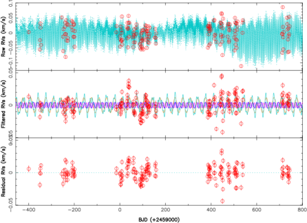
Figure 8: Same as Fig. 7 but including candidate planet e (orange and cyan curves for e and b+c+e in the middle plot) in the MCMC modeling. The RMS of the residuals is now 10.4 m s^-1.

Figure 9: Periodogram of the raw (top), filtered (middle) and residual (bottom) RVs when including candidate planet e (plus b and c) in the MCMC modeling. The cyan vertical dashed lines trace the rotation period of the star and the orbital periods of planets b and c, and of candidate planets d and e, while the horizontal dashed line indicate the 10 and 0.1% FAP levels in the periodogram of our RV data. The orange curve depicts the window function, whereas the orange vertical dashed and dotted line outline the 1-yr period, the synodic period of the Moon and its 1-yr aliases.

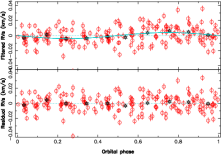
Figure 10: Filtered (top plot) and residual (bottom plot) RVs for transiting planets b (top panel) and c (middle panel), and for candidate planet e (bottom panel) of AU Mic. The red dots are the individual RV points with the respective error bars, whereas the black stars are average RVs over 0.1 phase bins. As in Fig. 8, the dispersion of RV residuals is 10.4 m s^-1.

We explored the possibility of an additional system planet whose RV signatures would still be hiding in our data. By looking at the periodogram of the filtered RV data, we find residual power at a period of 33.4 d that may hint at the presence of a candidate planet (dubbed planet e), which would be located further out close to a 4:1 resonance with planet b and 7:1 resonance with the rotation period of the host star. When candidate planet e is taken into account in the modeling and MCMC searches again for the most likely combination of activity and planet signatures, the 33.4 d peak dominates the periodogram of the filtered RVs at a level that corresponds to a false alarm probability (FAP) that the signal is spurious of order $10^{-10}$. We find an orbital period of $P_{e}=33.39\pm 0.10$ d and a semi-amplitude of $K_{e}=11.1^{+2.1}_{-1.7}$ m s^-1 for candidate planet e, i.e., about 2.5$\times$ larger than those of planets b and c. The RV signal is detected at a level of 6.5$\sigma$, with $\log\mathcal{L}_{M}$ increasing by 16.3 with respect to the reference case with planets b and c only, and the RMS of the RV residuals and the additional white noise $\theta_{5}$ both decreasing. With this model, the semi-amplitudes associated with planets b and c slightly increase, reaching now $K_{b}=4.5^{+1.7}_{-1.2}$ m s^-1 and $K_{c}=4.8^{+1.6}_{-1.2}$ m s^-1, implying a $\simeq$4$\sigma$ detection. The corresponding fit and periodogram are shown in Figs. 8 and 9, whereas the phase-folded filtered RV data for planets b, c and e are presented in Fig. 10 (both before and after binning on phase bins of 10 percent of their orbital cycles). No peak crosses the 10% FAP threshold in the residual RVs (see Fig.9 bottom plot). We note that the derived period for candidate planet e is close to a 1-yr alias of the synodic Moon period (32.1 d, visible in the periodogram of the window function, see Fig. 9), but distant from it by more than the FWHM of the periodogram peak, ensuring they are distinct. Adjusting eccentricities of all 3 planets yields again values consistent with 0 (error bars of 0.04, 0.07 and 0.09 for planets b, c and e respectively) and no more than a small increase in marginal logarithmic likelihood ($\Delta\log\mathcal{L}_{M}=0.8$), confirming that the model with circular orbits is enough to describe our RV data.

Although the periodogram of the RV residuals shows no obvious signal, we investigated whether our RV data could suggest the presence of additional planets beside candidate planet e, in particular the candidate planet d suggested by Wittrock et al. (2023) that may orbit between b and c and potentially explain the large TTVs reported for b and c. When including all 4 planets in the modeling (assuming again circular orbits), we find very similar results for b, c and e (see Table 4), and a very small semi-amplitude of $K_{d}=1.1^{+1.1}_{-0.5}$ m s^-1, which in fact amounts to a mere 3$\sigma$ upper limit on $K_{d}$ of 4.4 m s^-1. As expected, the marginal logarithmic likelihood increases very little ($\Delta\log\mathcal{L}_{M}=0.3$) when d is included in the modeling, implying that our data provide no evidence for its existence (within the quoted 3$\sigma$ upper limit).

We finally note that the parameters of the fitted GP are similar for all cases, except for the additional white noise ($\theta_{5}$) which decreases when adding planets b, c and e in the model. We find that the timescale on which the activity jitter evolves is longer than that on which $B_{\rm\ell}$ changes but similar to that associated with <$B$>. We also obtain that the rotation period derived from the activity jitter ($\theta_{2}=4.865\pm 0.005$ d) is marginally longer than the nominal one used to phase the data (4.86 d, see Table 1) and those derived from $B_{\rm\ell}$ and <$B$> measurements (respectively equal to $4.856\pm 0.003$ and $4.859\pm 0.004$ d). These periods indicate that the center of gravity of the surface features generating the activity jitter is located within the range of latitude 25–29^∘ (see Sec. 5.4). We point out that the smoothing factor $\theta_{4}$ derived from RV data is smaller than that inferred from $B_{\rm\ell}$ and <$B$>, as expected from the fact that RV is proportional to the derivative of the integrated flux (at first order), whereas $B_{\rm\ell}$ and <$B$> simply grow as the integral of the magnetic field vector / strength over the visible hemisphere. The periodogram of the filtered RVs (see Fig.9, middle plot) clearly demonstrates that activity filtering using GPR is quite efficient despite the long observing window, with no excess power remaining at the rotation period, harmonics and aliases.

7 Activity proxies of AU Mic

The main goal of this section is to investigate how the various activity proxies correlate with RVs, to find out whether one can be used to achieve a filtering of the activity jitter that is as accurate as, or even more efficient than, that achieved through GPR (see Sec. 6).

The first obvious activity proxy to investigate is the small-scale field <$B$>, already studied in Sec. 4 and reported to correlate well with RVs in the particular case of the Sun (Haywood et al., 2022). We find that RVs of AU Mic correlate poorly with $B_{\rm\ell}$ ($R=0.33$) and <$B$> ($R=0.12$), but nicely with the first time derivative of <$B$> (computed from the GPR fit to <$B$>, $R=0.78$). This is similar to what was reported by Suárez Mascareño et al. (2020) for Proxima, where RVs are found not to correlate with the FWHM of the cross-correlation profile, presumably linked to <$B$> via magnetic broadening, but with its first time derivative. This is also consistent with our finding that <$B$> correlates reasonably well with the FWHM of the Stokes $I$ profiles of high-Landé lines in AU Mic ($R=0.60$, see Sec. 4), but not with what was reported by Klein et al. (2021) in the particular case of the small late-2019 subset (where RVs correlated well with FWHMs). Altogether, it indicates that the activity jitter of M dwarfs like Proxima and AU Mic reflects the RV impact of brightness or magnetic features at the surface of the star, rather than the signature of inhibited convective blue-shift, expected to be much smaller for M dwarfs than for the Sun.

However, trying to directly filter out RVs of AU Mic using the first time derivative of <$B$> as a proxy to predict the activity jitter is less efficient than the GPR filtering outlined in Sec. 6. We find that the RV residuals are still modulated with rotation, albeit with an amplitude of about 45% that of the original jitter. The predicted RV jitter within each season is indeed not entirely consistent with the observed RVs, either in amplitude or in phase pattern, leaving residuals that still dominate the RV signatures from the 3 planets. Applying the same 3-planet plus QP GPR modeling as that of Sec. 6 on the filtered RVs yields results for the parameters of b, c and e and RV residuals that are very similar to those obtained in Sec. 6. It confirms that the RV signatures detected for all 3 planets are not a spurious artifact induced by activity, but brings no improvement in the RMS of RV residuals. We note that the periodogram of <$B$> only features a strong peak at the rotation period of AU Mic, and virtually no power at the orbital periods of the planets.

Looking now at the LBL activity proxy dLW, we find that it is modulated by rotation, with a QP GPR fit yielding a period of $4.88\pm 0.03$ d, consistent with AU Mic’s reference period of 4.86 d. The dispersion with respect to the fit is 3$\times$ larger than the median error bar of individual points (a likely result of intrinsic variability), whereas the modulation amplitude derived by GPR is only 25% larger than the dispersion. It is less useful in this respect than <$B$> or even the FWHM of the Stokes $I$ profiles of high-Landé lines, both exhibiting clearer rotational modulation (see Sec. 4). This difference likely comes from the fact that dLW, computed from all spectral lines (including molecular features, on average less sensitive to magnetic fields), is less appropriate for diagnosing small-scale magnetic fields than <$B$> or the FWHM of the Stokes $I$ LSD profiles of atomic lines with high Landé factors. We also note that RVs poorly correlate with dLW, as already reported for <$B$> and FWHMs.

Since dLW is measured on individual lines with LBL, one can carry out a weighted principal component analysis (wPCA, Delchambre, 2015) on the time series corresponding to all individual lines, to find out how temporal variations of line widths differ from line to line, as a likely impact of small-scale fields (Cadieux et al., in prep.). When applied to AU Mic, we find that the strongest wPCA component $W_{1}(t)$ is enough to explain most of the line-to-line differences, and that $W_{1}$ is clearly modulated with rotation, with a QP GPR yielding a recurrence period of $4.859\pm 0.003$ d and a decay time of $141\pm 15$ d, fully consistent with those derived for <$B$> (see lower section of Table 2). Furthermore, we find that that $W_{1}$ is strongly correlated with <$B$> ($R=0.96$). Unsurprisingly, using $W_{1}$ (instead of <$B$>) to filter RVs yields results very similar to those outlined above, i.e., an activity jitter reduced in amplitude by a factor of 2 compared to the original one, but still dominating the planet signatures. The RV planet signatures derived from the filtered RVs are again consistent with the values listed in Table 4.

We also measured equivalent width variations (EWVs) of the 1083 nm He i triplet and 1282 nm Pa${\beta}$ line, tracing stellar activity and potentially star-planet interactions (Klein et al., 2022), and whose profiles are shown in Fig. 15 (supplementary material). We proceeded as in Finociety et al. (2021, 2023), computing a median spectrum by which all spectra are divided, and fitting a Gaussian profile of fixed width and position (in the stellar rest frame) to the residual spectra. The derived values and error bars are listed in Table 5, with a few flares detected in He i but not in Pa${\beta}$. We find that both indices are modulated with the stellar rotation period. Fitting the EWVs with GPR yields periods of $4.86\pm 0.01$ d for both the He i and Pa${\beta}$ lines, when setting the decay time to 100 d (i.e., a value close to that derived from $B_{\rm\ell}$ data, see Sec. 4). In both cases, the excess white noise, quantifying the intrinsic variability of both activity indicators, is significantly larger than the formal photon-noise error bars (median of 0.030 and 0.015 km s^-1 for He i and Pa${\beta}$), by an order of magnitude or more, reaching 0.5 and 0.1 km s^-1 for He i and Pa${\beta}$. It confirms again the strong variability that AU Mic triggers at all times, especially in the He i line for which the semi-amplitude of the modulation is only about 70% the size of the excess white noise (whereas both are comparable in strength for Pa${\beta}$). While Pa${\beta}$ EWVs correlate reasonably well with <$B$> ($R=0.60$), it is not the case for He i EWVs that are much more dispersed, presumably as a result of intrinsic variability and chromospheric activity. We also find that the Pa${\beta}$ EWVs slowly decrease with time like <$B$> does, suggesting that AU Mic may be progressing towards activity minimum along its putative cycle (Ibañez Bustos et al., 2019).

As for <$B$>, the periodogram of the Pa${\beta}$ EWVs is featureless apart from the main peak at $P_{\rm rot}$ (with a FAP well below the 0.1% threshold). In particular, no signal shows up at the orbital periods of the planets. The periodogram of the He i EWVs is much more noisy, with again a main peak at $P_{\rm rot}$ (FAP of 0.1%). Multiple peaks are also present at a FAP level of 10% or higher, including at frequencies close to the orbital periods of transiting planets b and c. As these peaks do not correspond to a safe detection, and since similar peaks are also present at different periods throughout the periodogram, we conclude that their proximity with the orbital frequencies of planets b and c is no more than a coincidence.

All activity proxies discussed here exhibit rotational modulation, though with different levels of significance. However, even the best of them, i.e., <$B$> and $W_{1}$ (whose first time derivatives correlate well with RVs), are moderately successful at filtering the dominant activity jitter from the RV curve of AU Mic.

8 Summary and discussion

Our paper presents a detailed study of the young active star AU Mic based on 235 high-resolution unpolarized and circularly polarized spectra collected with SPIRou at CFHT from early 2019 to mid 2022, covering a timespan of 1,144 d over 4 successive seasons.

We revisited the main parameters of AU Mic, including its surface magnetic flux, using the median SPIRou spectrum, and found that $\hbox{$T_{\rm eff}$}=3665\pm 31$ K, $\hbox{$\log g$}=4.52\pm 0.05$, ${\rm[M/H]}=0.12\pm 0.10$ and $[\alpha/{\rm Fe}]=0.00\pm 0.04$. These parameters are consistent with a mass and radius of $0.60\pm 0.04$ ${\rm M}_{\odot}$ and $0.82\pm 0.02$ ${\rm R}_{\odot}$, respectively, at an age of $\simeq$20 Myr, in the context of the Baraffe et al. (2015) and Dotter et al. (2008) evolutionary models, except for the estimated $\log g$ that is larger (by about 3$\sigma$) than that expected from the mass and radius. Given the nominal rotation period of AU Mic (4.86 d), the projected rotation velocity $v\sin i$ is $8.5\pm 0.2$ km s^-1, consistent with previous literature estimates. Both evolutionary models further suggest that AU Mic already developed a small radiative core. The small-scale magnetic field <$B$>, adjusted with the atmospheric parameters on the median spectrum from a set of nIR lines with known Zeeman patterns (Cristofari et al., 2023), is equal to $2.61\pm 0.05$ kG, again consistent with previous literature measurements and typical to field strengths of active M dwarfs (e.g., Kochukhov & Reiners, 2020; Reiners et al., 2022). We find that modeling Zeeman broadening is important to derive accurate atmospheric parameters for strongly magnetic stars like AU Mic.

As in Klein et al. (2021), the large-scale magnetic field of AU Mic is detected through circularly polarized Zeeman signatures of atomic lines. The longitudinal field $B_{\rm\ell}$, probing the large-scale field, exhibits obvious rotational modulation with a period of $4.856\pm 0.003$ d. The corresponding pattern features a semi-amplitude ranging from 100 (in 2019) to 250 G (in 2020) and evolves on a timescale of $80\pm 12$ d, typical to largely- or fully-convective M dwarfs whose large-scale fields are usually stable over a few months (e.g., Morin et al., 2008a, b; Hébrard et al., 2016). The small-scale field <$B$> also exhibits rotational modulation though weaker than that of $B_{\rm\ell}$, with a different pattern (minimum and maximum amplitude in 2020 and 2021 respectively) and a slightly longer period of $4.859\pm 0.004$ d. The evolution timescale is about twice longer for <B> than for $B_{\rm\ell}$. The FWHM of the Stokes $I$ LSD profiles of atomic lines with high Landé factors comes as an alternate option for measuring <$B$>, albeit with a loss of precision.

Applying ZDI on the rotationally modulated sets of LSD Stokes $V$ profiles of each observing season, and setting the Doppler width of the local profile to $\hbox{$v_{\rm D}$}=5.3$ km s^-1 (to match the shape of the average LSD Stokes $I$ profile with minimal Zeeman broadening), we find that the large-scale field of AU Mic reaches $\simeq$400 G, is mainly poloidal and axisymmetric, and with a dipole component of $\simeq$400 G tilted at 15–50^∘ with respect to the rotation axis depending on the season. Optimal results are obtained for a filling factor of the large-scale field $f_{V}\simeq 0.2$. If we include Stokes $I$ LSD profiles in the fitting procedure as well and further assume that the local small-scale field scales up with the local large-scale field (with the filling factor of the small-scale field set to $f_{I}\simeq 0.9$ and the Doppler width of the local profile to a more conventional value of $\hbox{$v_{\rm D}$}=3.5$ km s^-1), we find that a stronger large-scale field of $\simeq$550 G and a small-scale field of $\simeq$2.5 kG are needed to simultaneously reproduce LSD Stokes $V$ and $I$ profiles. The reconstructed field is even more poloidal and axisymmetric, with a dipole component of $\simeq$650 G only moderately tilted with respect to the rotation axis (by 10^∘ to 25^∘). This magnetic topology is consistent with those of fully or largely convective main-sequence M dwarfs, whose convective zone is deeper than about half the stellar radius (Donati & Landstreet, 2009), whereas the ratio of magnetic flux between small and large scales ($f_{V}/f_{I}=0.22$) agrees with previous measurements (Morin et al., 2008b; Kochukhov, 2021).

Whereas the Stokes $I$ & $V$ analysis gives a more reliable description of the overall strength and geometry of the average large-scale and small scale fields at the surface of AU Mic, the Stokes $V$ analysis better accounts for the seasonal evolution of the large-scale field. The difference in large-scale field strength between these two approaches reflects that some of the large-scale magnetic topology of AU Mic (and in particular the axisymmetric component) may remain undetected through Stokes $V$ data only, as a result of the almost perpendicular orientation of the stellar rotation axis with respect to the line of sight (assuming that the orbital plane of the planets coincides with the equatorial plane of the star). Collecting Stokes $Q$ and $U$ (in addition to Stokes $V$) data of AU Mic would help in this respect, as these Zeeman signatures should be detectable in AU Mic and could be used to efficiently differentiate between both magnetic configurations (see Fig. 14). An accurate estimate of the large-scale dipole field of AU Mic is also needed for studies of potential interactions between the host star and its close-in planets (Kavanagh et al., 2021; Klein et al., 2022), or for space weather simulations in the system (Carolan et al., 2020; Alvarado-Gómez et al., 2022; Mesquita et al., 2022).

From the temporal evolution of Stokes $V$ profiles in 2020 and 2021, we retrieve the average amount of latitudinal differential rotation shearing the surface of AU Mic, and find that the rotation rate at the equator $\Omega_{\rm eq}$ and the difference in rotation rate between the equator and pole $d\Omega$ are equal to 1.299 and 0.037 rad d^-1, corresponding to rotation periods at the equator and pole of 4.84 and 4.98 d, respectively, and to a latitudinal shear equal to about two thirds that at the surface of the Sun. This amount of DR is typical to that found on partly convective low-mass stars (e.g., Hébrard et al., 2016). As the values derived at each epoch ($\hbox{$\Omega_{\rm eq}$}=1.3006\pm 0.0004$ and $\hbox{$d\Omega$}=0.0445\pm 0.0014$ rad d^-1 in 2020 and $\hbox{$\Omega_{\rm eq}$}=1.2970\pm 0.0002$ and $\hbox{$d\Omega$}=0.0298\pm 0.0013$ rad d^-1 in 2021) differ by more than 3$\sigma$, we can conclude that differential rotation at the surface of AU Mic is likely varying with time. We nonetheless caution that the unusual amount of intrinsic variability observed for this star may have induced part of this discrepancy, making it essential to monitor the star over at least several months to minimize its impact and ensure we can derive reliable estimates of the DR parameters.

RVs inferred with the LBL technique (Artigau et al., 2022) from the SPIRou spectra of AU Mic processed with APERO (Cook et al., 2022) show an overall scatter of 31 m s^-1 RMS over the full observing period, with some seasons (e.g., 2020) exhibiting a smaller than average dispersion (24 m s^-1). This is a factor of about 4 smaller than the average scatter at visible wavelengths (127 m s^-1 RMS) reported by Zicher et al. (2022), illustrating how efficient SPIRou is to obtain precise RVs of active M dwarfs (e.g., Carmona et al., 2023). These RV variations are strongly modulated with a period of $4.866\pm 0.004$ d, marginally longer than that on which $B_{\rm\ell}$ and <$B$> are modulated. We further obtain that RVs are well correlated, neither with $B_{\rm\ell}$ nor with <$B$> but with the first time derivative of <$B$> ($R=0.78$), similar to what was reported for Proxima (using the FWHM of the cross-correlation function as a proxy for <$B$>, Suárez Mascareño et al., 2020). Using this correlation to filter RVs from the activity jitter improves the situation but leaves a significant fraction (about 45%) of the jitter. A QP GPR fit to the RVs provides a more efficient filtering, leaving essentially no signal at the rotation period and its harmonics and aliases. The typical evolution timescale of the activity jitter is found to be $136\pm 21$ d, larger than that of $B_{\rm\ell}$ but consistent with that of <$B$>. Although the dLW activity index provided by LBL does not correlate well with <$B$>, we find that the strongest wPCA component $W_{1}(t)$ of all per-line dLW time series is strongly correlated with <$B$> in AU Mic ($R=0.96$) and can thereby serve as a much better activity proxy than dLW itself (Cadieux et al., in prep.). Filtering RVs using the first time derivative of $W_{1}$ yields results similar to (though not better than) those achieved with <$B$>. Machine Learning is apparently a promising alternative to GPR for filtering activity (Perger et al., 2023), with the advantage of being based on a physical background.

Modeling the RV signatures of transiting planets b and c (with the orbital periods and TESS transit times set to the values quoted in Szabó et al., 2022) at the same time as the activity jitter yields semi-amplitudes of $K_{b}=4.1^{+1.8}_{-1.2}$ m s^-1 and $K_{c}=4.0^{+1.7}_{-1.2}$ m s^-1 for planets b and c, with a residual RV scatter of 11.1 m s^-1 RMS. This is consistent with previous results from optical data (where the activity jitter is 4$\times$ larger, Zicher et al., 2022) for planet b, but smaller by a factor of 2 for planet c. We suspect that the difference mainly reflects residuals when filtering the strong activity jitter from optical data, that resulted in relatively large error bars on the semi-amplitudes of both planets (of 2.5 m s^-1, i.e., 1.5–2$\times$ larger than ours). When looking at residuals in the periodogram of filtered RVs, we find excess power at a period of 33.4 d that hints at the presence of another planet in the system, dubbed candidate planet e. Fitting orbital parameters of planet e along with those of planets b and c and the hyper-parameters of the GP describing activity yields $K_{e}=11.1^{+2.1}_{-1.7}$ m s^-1 and $P_{e}=33.39\pm 0.10$ d, and slightly larger semi-amplitudes for planets b and c ($K_{b}=4.5^{+1.7}_{-1.2}$ m s^-1, $K_{c}=4.8^{+1.6}_{-1.2}$ m s^-1), with the RV signatures detected at a 6.5$\sigma$ level for planet e and $\simeq$4$\sigma$ level for b and c. We find that including candidate planet e gives a logarithmic Bayes factor of 16.3 for this model with respect to that featuring planets b and c only (plus activity), indicating that the detection is reliable, and induces a decrease in the residual RV scatter (now 10.4 m s^-1 RMS). Fitting eccentricities of all 3 planets yields values compatible with zero (with error bars of 0.04, 0.07 and 0.09 for planets b, c and e respectively) along with a non-significant increase in marginal logarithmic likelihood, confirming that circular orbits for all 3 planets is the default model to be used here. We stress that the period of candidate planet e is close to a 1-yr alias of the Moon synodic period (32.1 d, see window function in Fig. 9) but distant from it by 13$\times$ the error bar on the derived period, ensuring that both peaks are distinct. We nonetheless caution that this proximity is suspicious, hence why we choose to refer to planet e as a candidate planet at this stage. We also note that candidate planet e is close to a 4:1 resonance with planet b, and to a 7:1 resonance with the rotation of the star.

The derived semi-amplitudes yield masses of $10.2^{+3.9}_{-2.7}$, $14.2^{+4.8}_{-3.5}$ and $35.2^{+6.7}_{-5.4}$ ${\rm M}_{\oplus}$ for planets b, c and e, respectively. The corresponding densities for planets b and c (whose radii are $3.55\pm 0.13$ and $2.56\pm 0.12$ ${\rm R}_{\oplus}$, where ${\rm R}_{\oplus}$ notes the Earth radius Szabó et al., 2022) are $1.26^{+0.68}_{-0.43}$ and $4.7^{+2.5}_{-1.6}$ g cm^-3, i.e., about 3.7$\times$ larger for c than for b whereas the opposite is usually observed in evolved multi-planet systems (but not for all, e.g., Leleu et al., 2021) as a result of the difference in equilibrium temperatures ($593\pm 21$ and $454\pm 16$ K for b and c respectively, Martioli et al., 2021, $\simeq$370 K for candidate planet e using similar assumptions). However, the observed density contrast also reflects the fact that both planets did not yet complete their contraction process, in particular planet b that is still rather inflated (Zicher et al., 2022). Both planets are not expected to evolve in the same way as a result of cooling, contraction or photo-evaporation of the H/He atmosphere, given the difference in mass and distance from the star. In particular, given its higher equilibrium temperature possibly boosted by induction heating (Kislyakova et al., 2018), and its marginally lower mass, b is expected to increase its density more than c, hence reducing the density contrast between both. Predicting the evolution of b and c from their observed positions in a radius versus mass diagram (see Fig. 11) requires calculations with, e.g., the MESA models (Owen & Wu, 2013), as in Zicher et al. (2022). The inflation of planet b makes it an ideal target for future atmospheric characterization, especially given its strong level of irradiation that should also extend its atmosphere and provide opportunities of investigating deeper atmospheric layers (García Muñoz et al., 2021). Whereas planet e alone should place the planetary system of AU Mic in the ’ordered’ category recently defined by Mishra et al. (2023), planet d and e should put it in the ’mixed’ class. In both cases, AU Mic will bring valuable observational constraints on young planetary system architectures and their expected evolution with time.

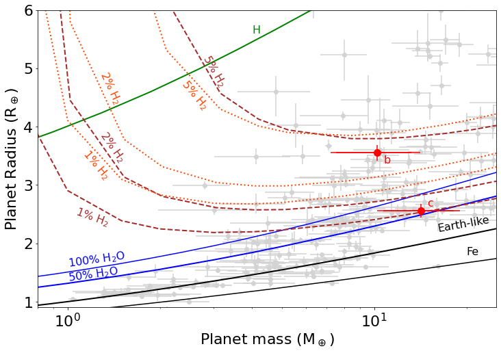
Figure 11: Mass-radius diagram for exoplanets whose mass and radius are known with a relative precision better than 30% (grey points). AU Mic b and c are shown with red filled circles and corresponding error bars, and are expected to contract with age (e.g., Owen & Wu, 2013). Theoretical models of Zeng et al. (2016); Zeng et al. (2019) corresponding to various inner planet structures / compositions are depicted with black (100% iron and Earth-like), green (100% H) and blue (100% and 50% H₂O envelope) full lines. Models with a 1%, 2% and 5% H₂ atmosphere with either an Earth-like (brown dashes) or a 50% water (orange dashes) interior are also shown.

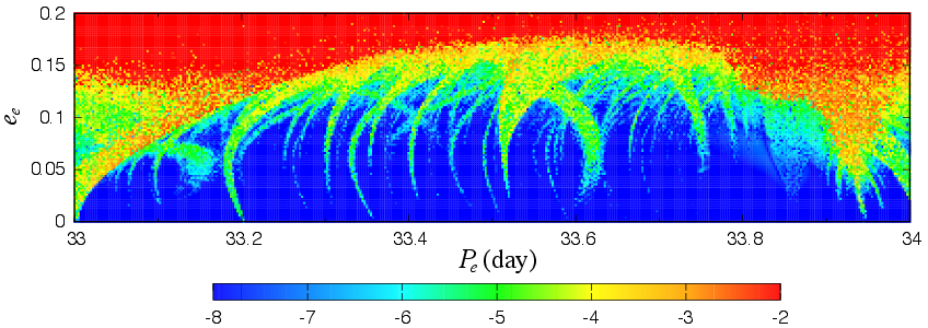
Figure 12: Period versus eccentricity stability diagram for candidate planet e of the b+c+e AU Mic system. The phase space of the system is explored by varying the period (in d) and eccentricity of candidate planet e about the value derived in this work (Table 4). For each initial condition, the system is integrated over 5 kyr with the symplectic integrator SABAC4 (Laskar & Robutel, 2001). A stability criterion is derived from the frequency analysis of the mean longitude (Laskar, 1993). The chaotic behaviour is quantified by the variation in the mean motion, with the color scale coding the decimal logarithm of the mean motion variation (Correia et al., 2010). The red areas corresponds to unstable orbits, and the blue ones to orbits that are presumably stable on a Gyr timescale.

Assuming it is located in the same orbital plane as transiting planets b and c and given the impact parameters of b and c (respectively equal to $0.17\pm 0.11$ and $0.58\pm 0.13$ $R_{\star}$, Szabó et al., 2022), candidate planet e is probably not transiting or only through a grazing transit given the distance at which it orbits, i.e., $0.171\pm 0.005$ au, as opposed to $0.0645\pm 0.0013$ and $0.1101\pm 0.0022$ au for planets b and c. No transit at this period has been reported yet, although the limited monitoring windows of TESS for AU Mic (28 d) would make it more difficult to detect (if it happens) than those of planets b and c. We note that the derived epoch of transit (or of conjunction) implies that if planet e is transiting, several transits should have been observed in TESS data (in sector #1 at BJD $2458449.3\pm 2.9$ and sector #27 at BJD $2459050.3\pm 1.1$) and potentially during CHEOPS #2 and #3 visits as well (at BJDs $2459083.7\pm 1.0$ and $2459117.1\pm 0.9$, Szabó et al., 2021). Since these data show no evidence of a transit, we conclude that candidate planet e is unlikely to transit.

By studying the stability of the b+c+e system, we find that candidate planet e can be stable on a Gyr timescale for the orbital periods and modest eccentricities allowed by the RV data (see Fig. 12). The best fit orbital solution (see Table 4) is not in exact resonance with any of the other planets, implying that planet e is not able to significantly perturb the orbits of planets b and c nor to generate the TTVs of up to $\pm$10 min reported for planet b (Szabó et al., 2022). By scanning a range of values about those derived in our study for the parameters of planet e (mass, period, eccentricity, and argument of periastron) to investigate whether a reasonable fit to the observed TESS, Spitzer and CHEOPS transit epochs was achievable, we obtain that no combination is able to reproduce transit data, even for orbital periods corresponding to a 4:1 resonance with planet b.

We also investigated whether candidate planet d, suggested to be orbiting between b and c and potentially causing the reported TTVs (Wittrock et al., 2023), is detectable in our data. We find no clear evidence of its presence and derive a 3$\sigma$ upper limit on the amplitude of its RV signature ($K_{d}<4.4$ m s^-1) and on its minimum mass ($M_{d}<11.4$ ${\rm M}_{\oplus}$), consistent with the prediction ($\simeq$1 ${\rm M}_{\oplus}$, Wittrock et al., 2023). Besides, we confirm that b+c+d is stable for the 12.74-d period and low-eccentricity orbit of planet d suggested by Wittrock et al. (2023), whereas b+c+d+e, though less stable, should still be able to survive on long timescales (see Fig. 16 in supplementary material). We also verified that the simulated TTVs are much more consistent with the transit timings of planets b and c once candidate planet d is included (see Fig. 17 in supplementary material, in agreement with Wittrock et al., 2023).

Finally, we studied the Pa${\beta}$ and He i lines and in particular the temporal modulation of their equivalent widths (EWVs) over our 4 observing seasons. We find that these lines exhibit clear modulation with periods that are consistent with the rotation period of the star, despite showing both a significant level of intrinsic variability. EWVs are clearer for Pa${\beta}$ (than for He i) and are found to correlate reasonably well, for this line, with our estimates of the small-scale field <$B$>. Both Pa${\beta}$ EWVs and <$B$> slowly decrease with time over the 3 yr of our observing campaign, suggesting that AU Mic may be progressing towards activity minimum along its putative cycle (Ibañez Bustos et al., 2019). As opposed to Klein et al. (2022), we find no clear evidence that either line is modulated at the period of the system planets. The low-significance peaks (FAP of $\simeq$10%) observed close to the orbital periods of planets b and c in the periodogram of He i EWVs are similar in strength to many others and cannot reliably be considered as a sign of, e.g., star-planet interaction between AU Mic and its inner planets.

We will pursue our spectropolarimetric monitoring of AU Mic with SPIRou for another 2 yr within the context of the new SPICE Large Programme, that was allocated 175 nights of CFHT time from late 2022 to mid 2024, and whose aim is to consolidate and enhance the results of the SLS. The first goal is to firmly ascertain the existence of candidate planets e and possibly d, and improve at the same time the precision on the mass estimates of all planets, a rather tricky task given the extreme activity level of AU Mic, even in the nIR where the RV activity jitter is 4$\times$ smaller than at visible wavelengths. With its system of young planets (2 of which transiting) that are still likely evolving with time, AU Mic is an ideal laboratory to test and constrain models of planet formation and evolution, and to investigate the atmospheric composition of young inflated planets. Besides, we also aim at pursuing the magnetic monitoring of AU Mic on a longer timescale to investigate whether the poloidal and toroidal components of large-scale field vary in a cyclic way (e.g., Ibañez Bustos et al., 2019), switching sign as they do on the Sun, and to document the changes in the small-scale field as the large-scale field evolves with time. Given that no clear sign switch was observed yet in either field component, the present data suggest that, if there is a cycle, the period is at least 5 years. We stress that having access to Stokes $Q$ and $U$ observations of AU Mic with SPIRou for at least a partial season, and thereby complement the Stokes $V$ and $I$ data to be collected with SPICE, would further enhance our ability to consistently model the magnetic topology and verify the assumptions on which the results presented in this paper rely. More generally, multi-wavelength, multi-instrument monitoring campaigns of AU Mic, involving in particular precision photometry from space (TESS, CHEOPS and later-on PLATO), optical and nIR high-resolution spectropolarimetry and velocimetry (e.g., ESPaDOnS, SPIRou, CRIRES+ for longer wavelengths), and low-resolution nIR spectroscopy from space with the JWST, especially during transits, would be a must to characterize in detail this young multi-planet system of our immediate neighbourhood.

Data availability

Most data underlying this paper are part of the SLS, and will be publicly available from the Canadian Astronomy Data Center by February 2024, while the PI and DDT data are already public.

Appendix A Observation log

Table 5 outlines the full observation log, as well as all individual measurements carried out from the collected spectra at each epoch.

Table 5: Observation log. All exposures consist of 4 sub-exposures of equal length, except that marked with an ‘x’ for which only 2 of the 4 sub-exposures could be used. For each visit, we list the corresponding barycentric Julian date BJD, rotation cycle c and phase $\phi$ (computed as indicated in Sec. 2), the total observing time t_exp, the peak SNR in the spectrum, the noise level in the LSD Stokes $V$ profile, the estimated $B_{\rm\ell}$ and <$B$> with error bars, the RV and error bar estimated by LBL whenever relevant (once per night) and available, the wPCA component $W_{1}$ derived from the LBL dLW proxy (see text), and the EWVs as measured in the He i and Pa${\beta}$ lines. Exposures affected with a flare (detected in the He i line) are marked with a ‘+’.

BJD	c / $\phi$	texp	SNR	$\sigma_{V}$	$B_{\rm\ell}$	<$B$>	RV	$W_{1}$	EWV He i	EWV Pa${\beta}$
(2459000+)		(s)		($10^{-4}I_{c}$)	(G)	(kG)	(m s-1)	(km2 s-2)	(km s-1)	(km s-1)
-399.8747695	-83 / 0.721	378.9	427	1.53	-68.6$\pm$8.2		2.7$\pm$4.9	-1.32$\pm$0.13	0.749$\pm$0.077	0.269$\pm$0.033
+ -350.8732586	-73 / 0.804	763.4	752	1.19	-63.3$\pm$6.4	2.89$\pm$0.03	-55.2$\pm$4.6	-1.24$\pm$0.11	3.111$\pm$1.045	0.218$\pm$0.019
-349.8781098	-72 / 0.009	741.1	753	1.14	-27.4$\pm$6.0	2.59$\pm$0.02	-24.0$\pm$3.5	1.15$\pm$0.12	0.405$\pm$0.043	-0.032$\pm$0.019
-348.9179834	-72 / 0.206	735.5	753	1.36	123.9$\pm$7.3	2.69$\pm$0.02	31.7$\pm$3.7	0.43$\pm$0.12	0.438$\pm$0.042	-0.231$\pm$0.018
-348.0685108	-72 / 0.381	490.3	407	1.73	82.8$\pm$9.6				-0.407$\pm$0.073	0.138$\pm$0.031
-348.0607403	-72 / 0.383	490.3	451	1.60	67.7$\pm$8.9				-0.233$\pm$0.068	0.020$\pm$0.027
-348.0539511	-72 / 0.384	490.3	511	1.36	74.2$\pm$7.6				-0.387$\pm$0.066	-0.086$\pm$0.028
-348.0466565	-72 / 0.385	490.3	532	1.33	67.2$\pm$7.4				-0.252$\pm$0.068	0.071$\pm$0.029
-348.0392277	-72 / 0.387	490.3	519	1.31	76.5$\pm$7.2				-0.196$\pm$0.069	0.047$\pm$0.029
-348.0319186	-72 / 0.388	490.3	523	1.36	85.0$\pm$7.5				-0.216$\pm$0.067	0.073$\pm$0.029
-348.0247451	-72 / 0.390	490.3	509	1.37	70.6$\pm$7.5				-0.290$\pm$0.081	0.029$\pm$0.033
-348.0172993	-72 / 0.392	490.3	523	1.33	64.8$\pm$7.2				-0.079$\pm$0.065	0.097$\pm$0.027
-348.0099247	-72 / 0.393	490.3	545	1.29	64.5$\pm$7.0				-0.227$\pm$0.069	-0.026$\pm$0.028
-348.0028446	-72 / 0.394	490.3	545	1.27	69.5$\pm$6.9				-0.159$\pm$0.075	0.081$\pm$0.032
-347.9953218	-72 / 0.396	490.3	523	1.31	54.1$\pm$7.1				-0.409$\pm$0.071	0.088$\pm$0.030
-347.9880112	-72 / 0.398	490.3	551	1.35	83.1$\pm$7.2	2.73$\pm$0.02	18.5$\pm$0.8	-0.34$\pm$0.12	-0.300$\pm$0.069	0.024$\pm$0.029
-347.9807843	-72 / 0.399	490.3	546	1.29	73.2$\pm$6.9				-0.173$\pm$0.070	-0.050$\pm$0.029
-347.9734398	-72 / 0.401	490.3	518	1.31	62.0$\pm$7.0				-0.009$\pm$0.063	0.077$\pm$0.027
-347.9660598	-72 / 0.402	490.3	527	1.32	57.6$\pm$7.1				-0.124$\pm$0.066	0.029$\pm$0.028
-347.9589404	-72 / 0.404	490.3	539	1.34	52.8$\pm$7.2				-0.207$\pm$0.067	0.066$\pm$0.029
-347.9515016	-72 / 0.405	490.3	536	1.34	58.5$\pm$7.2				-0.049$\pm$0.088	-0.007$\pm$0.036
-347.9442715	-72 / 0.407	490.3	506	1.36	64.9$\pm$7.2				-0.311$\pm$0.067	0.040$\pm$0.028
-347.9368452	-72 / 0.408	490.3	497	1.39	42.4$\pm$7.4				-0.063$\pm$0.066	0.057$\pm$0.028
-347.9298065	-72 / 0.410	490.3	499	1.45	48.4$\pm$7.7				-0.093$\pm$0.063	0.041$\pm$0.027
-347.9221049	-72 / 0.411	490.3	462	1.48	52.7$\pm$7.9				-0.172$\pm$0.062	-0.071$\pm$0.026
-347.9149019	-72 / 0.413	490.3	469	1.45	45.2$\pm$7.7				-0.292$\pm$0.062	-0.037$\pm$0.026
-347.9074044	-72 / 0.414	490.3	481	1.44	54.6$\pm$7.7				-0.278$\pm$0.062	0.038$\pm$0.026
-347.9002434	-72 / 0.416	490.3	501	1.45	46.2$\pm$7.8				-0.277$\pm$0.062	0.038$\pm$0.026
-347.8927767	-72 / 0.417	490.3	505	1.42	51.8$\pm$7.5				-0.157$\pm$0.062	0.048$\pm$0.027
-347.8854737	-72 / 0.419	490.3	518	1.38	53.7$\pm$7.4				-0.434$\pm$0.065	-0.005$\pm$0.027
-347.8782414	-72 / 0.420	490.3	531	1.33	43.7$\pm$7.1				-0.176$\pm$0.065	-0.069$\pm$0.028
-347.8710231	-72 / 0.422	490.3	535	1.38	52.4$\pm$7.3				-0.218$\pm$0.067	0.011$\pm$0.028
-347.8636629	-72 / 0.423	490.3	522	1.35	34.4$\pm$7.2				-0.286$\pm$0.062	-0.036$\pm$0.026
-345.9614621	-72 / 0.815	752.2	748	1.10	-55.9$\pm$6.0	2.87$\pm$0.03	-40.3$\pm$2.9	-1.07$\pm$0.13	0.259$\pm$0.043	0.136$\pm$0.019
-255.1779946	-53 / 0.494	780.1	731	1.00	-66.8$\pm$5.6	2.77$\pm$0.01	51.7$\pm$4.3	-0.47$\pm$0.10	0.062$\pm$0.044	-0.179$\pm$0.019
-249.2450248	-52 / 0.715	780.1	765	1.16	42.3$\pm$6.7	3.01$\pm$0.03	-12.7$\pm$5.0	-1.69$\pm$0.11	0.658$\pm$0.041	0.387$\pm$0.017
-248.2538870	-52 / 0.919	780.1	769	1.07	12.3$\pm$5.7	2.74$\pm$0.03	-60.8$\pm$4.2	-0.40$\pm$0.10	0.568$\pm$0.042	-0.169$\pm$0.018
-247.2094110	-51 / 0.134	780.1	763	1.00	75.5$\pm$5.3	2.57$\pm$0.03	12.6$\pm$4.3	1.40$\pm$0.10	0.114$\pm$0.041	-0.156$\pm$0.017
-241.2704220	-50 / 0.356	780.1	706	0.96	16.4$\pm$5.1	2.65$\pm$0.03	20.7$\pm$3.7	0.36$\pm$0.09	-0.638$\pm$0.046	-0.165$\pm$0.020
-240.1938818	-50 / 0.577	780.1	648	1.03	21.6$\pm$5.6	2.93$\pm$0.03	34.6$\pm$3.7	-1.41$\pm$0.10	0.417$\pm$0.054	0.028$\pm$0.022
-239.2714096	-50 / 0.767	780.1	580	1.17	45.6$\pm$6.3	2.94$\pm$0.03	-3.6$\pm$3.8	-1.50$\pm$0.11	0.781$\pm$0.064	0.106$\pm$0.026
-238.2687216	-50 / 0.974	780.1	757	1.01	-1.4$\pm$5.2	2.68$\pm$0.03	-80.4$\pm$4.3	0.18$\pm$0.10	0.647$\pm$0.044	0.079$\pm$0.018
-237.2676540	-49 / 0.179	780.1	749	0.94	79.6$\pm$4.9	2.63$\pm$0.03	-4.0$\pm$4.0	0.96$\pm$0.10	0.247$\pm$0.044	-0.109$\pm$0.019
-235.2421162	-49 / 0.596	780.1	759	1.26	31.2$\pm$7.0	2.96$\pm$0.03	42.6$\pm$4.5	-1.71$\pm$0.11	0.245$\pm$0.041	0.226$\pm$0.018
-234.2298202	-49 / 0.805	780.1	764	1.04	13.8$\pm$5.8	2.97$\pm$0.03	-25.3$\pm$4.3	-1.59$\pm$0.10	0.713$\pm$0.042	-0.011$\pm$0.018
-230.2553866	-48 / 0.622	780.1	767	1.02	42.8$\pm$5.6	2.99$\pm$0.03	29.8$\pm$4.3	-1.71$\pm$0.10	-0.002$\pm$0.044	0.158$\pm$0.018
-229.2585186	-48 / 0.827	780.1	702	1.11	20.7$\pm$6.0	2.90$\pm$0.03	-16.6$\pm$4.2	-1.21$\pm$0.10	0.338$\pm$0.047	0.070$\pm$0.020
-228.2780477	-47 / 0.029	780.1	697	1.03	5.1$\pm$5.6	2.65$\pm$0.03	-26.0$\pm$4.1	0.50$\pm$0.10	0.958$\pm$0.046	-0.182$\pm$0.020
-227.2576342	-47 / 0.239	780.1	665	1.12	82.2$\pm$6.3	2.65$\pm$0.02	26.9$\pm$4.3	0.41$\pm$0.10	-0.084$\pm$0.051	-0.144$\pm$0.021
-212.2836795	-44 / 0.320	780.1	650	1.09	-6.9$\pm$5.9	2.74$\pm$0.02	20.1$\pm$4.0	0.22$\pm$0.10	-0.625$\pm$0.051	-0.194$\pm$0.021
-211.2946856	-44 / 0.524	780.1	673	1.06	-7.8$\pm$5.9	2.90$\pm$0.03	40.3$\pm$4.2	-0.95$\pm$0.11	-0.769$\pm$0.050	0.014$\pm$0.021
-210.2625258	-44 / 0.736	780.1	740	1.00	106.4$\pm$5.6	2.98$\pm$0.03		-1.87$\pm$0.10	0.248$\pm$0.043	0.121$\pm$0.018
-209.2981790	-44 / 0.935	780.1	757	1.21	-13.2$\pm$6.7	2.76$\pm$0.02		-0.38$\pm$0.11	0.811$\pm$0.042	0.077$\pm$0.018
-208.3008722	-43 / 0.140	780.1	747	0.96	58.3$\pm$5.1	2.55$\pm$0.02	9.3$\pm$4.2	1.02$\pm$0.10	0.734$\pm$0.042	-0.013$\pm$0.018
-207.3015996	-43 / 0.345	780.1	778	1.08	-42.1$\pm$5.8	2.69$\pm$0.02	36.2$\pm$4.0	0.34$\pm$0.10	-0.910$\pm$0.041	-0.212$\pm$0.018
-203.3133195	-42 / 0.166	780.1	586	1.23	59.1$\pm$6.7	2.64$\pm$0.02	-12.9$\pm$4.3	0.86$\pm$0.11	-0.251$\pm$0.058	0.016$\pm$0.023
x -202.3142043	-42 / 0.372	390.0	424	1.73	-59.8$\pm$10.1				-1.426$\pm$0.059	0.078$\pm$0.024
-202.2674475	-42 / 0.381	780.1	593	1.19	-70.2$\pm$6.9	2.72$\pm$0.02	27.0$\pm$4.3	0.37$\pm$0.11	-1.282$\pm$0.082	0.059$\pm$0.033
-201.3118745	-42 / 0.578	780.1	631	1.07	85.8$\pm$6.0	2.88$\pm$0.02	29.8$\pm$3.8	-1.51$\pm$0.10	-0.540$\pm$0.054	0.111$\pm$0.022

Table 1: continued

BJD	c / $\phi$	texp	SNR	$\sigma_{V}$	$B_{\rm\ell}$	<$B$>	RV	$W_{1}$	EWV He i	EWV Pa${\beta}$
(2459000+)		(s)		($10^{-4}I_{c}$)	(G)	(kG)	(m s-1)	(km2 s-2)	(km s-1)	(km s-1)
-200.3108791	-42 / 0.784	780.1	579	1.19	91.7$\pm$6.8	2.93$\pm$0.03	-13.2$\pm$4.3	-1.59$\pm$0.11	0.044$\pm$0.060	0.280$\pm$0.025
-199.3096404	-42 / 0.990	780.1	746	1.00	-16.9$\pm$5.5	2.68$\pm$0.03	-46.4$\pm$4.1	-0.04$\pm$0.10	0.010$\pm$0.044	0.031$\pm$0.019
-198.3118516	-41 / 0.195	780.1	721	1.12	67.2$\pm$6.1	2.66$\pm$0.03	6.1$\pm$4.6	0.90$\pm$0.11	0.252$\pm$0.045	-0.200$\pm$0.019
-15.8798518	-4 / 0.733	780.1	701	0.94	196.7$\pm$5.2	2.77$\pm$0.03	2.2$\pm$3.6	-0.21$\pm$0.09	-0.062$\pm$0.045	0.174$\pm$0.019
-14.8996031	-4 / 0.934	780.1	736	0.90	-5.5$\pm$4.8	2.81$\pm$0.03	22.9$\pm$3.8	-0.74$\pm$0.09	0.343$\pm$0.042	0.153$\pm$0.018
+ 0.0859254	0 / 0.018	780.1	785	0.92	33.0$\pm$5.0	2.83$\pm$0.03	-11.5$\pm$4.2	-0.58$\pm$0.10	4.757$\pm$1.040	0.038$\pm$0.017
1.0109417	0 / 0.208	735.5	787	0.93	-75.8$\pm$4.9	2.72$\pm$0.03	-45.7$\pm$4.4	0.67$\pm$0.10	0.333$\pm$0.039	-0.173$\pm$0.017
3.0657407	0 / 0.631	780.1	764	1.14	211.0$\pm$6.4	2.71$\pm$0.03	-22.1$\pm$4.2	0.22$\pm$0.10	-0.349$\pm$0.039	0.016$\pm$0.017
4.0703036	0 / 0.838	780.1	760	0.94	83.5$\pm$5.1	2.82$\pm$0.03	21.6$\pm$4.1	-0.94$\pm$0.10	0.088$\pm$0.040	-0.074$\pm$0.017
5.0685152	1 / 0.043	774.5	774	0.87	31.9$\pm$4.7	2.79$\pm$0.03	-26.0$\pm$4.0	-0.53$\pm$0.09	0.266$\pm$0.039	-0.009$\pm$0.017
6.0994963	1 / 0.255	780.1	777	0.85	-149.0$\pm$4.4	2.70$\pm$0.02	-26.7$\pm$3.9	1.17$\pm$0.10	-0.369$\pm$0.040	0.060$\pm$0.017
7.0806725	1 / 0.457	757.8	785	0.85	-37.0$\pm$4.3	2.72$\pm$0.03	8.9$\pm$4.0	-0.60$\pm$0.10	-0.224$\pm$0.039	-0.392$\pm$0.016
8.0635561	1 / 0.659	774.5	777	0.90	221.5$\pm$4.7	2.72$\pm$0.03	0.2$\pm$3.6	0.41$\pm$0.09	-0.410$\pm$0.040	0.046$\pm$0.017
+ 9.0639632	1 / 0.865	780.1	740	0.95	55.8$\pm$5.1	2.82$\pm$0.03	55.0$\pm$4.0	-0.75$\pm$0.10	2.526$\pm$1.043	0.240$\pm$0.018
10.0304082	2 / 0.064	780.1	705	1.05	33.8$\pm$5.8	2.72$\pm$0.03	-39.1$\pm$3.8	-0.64$\pm$0.10	0.060$\pm$0.042	0.060$\pm$0.018
11.0027820	2 / 0.264	780.1	747	0.92	-164.4$\pm$5.1	2.64$\pm$0.03	-23.4$\pm$4.0	1.04$\pm$0.10	1.847$\pm$0.042	-0.051$\pm$0.018
31.0278512	6 / 0.384	707.6	789	0.98	-201.9$\pm$5.1	2.69$\pm$0.03	19.4$\pm$4.1	0.61$\pm$0.10	-0.991$\pm$0.035	-0.088$\pm$0.016
32.0334169	6 / 0.591	796.8	781	1.01	225.2$\pm$5.5	2.66$\pm$0.03	-18.0$\pm$4.0	0.26$\pm$0.09	-0.452$\pm$0.035	-0.047$\pm$0.017
33.0034293	6 / 0.791	802.4	797	0.84	106.7$\pm$4.5	2.76$\pm$0.03	33.9$\pm$3.9	-0.23$\pm$0.09	0.057$\pm$0.035	0.109$\pm$0.016
34.0637925	7 / 0.009	802.4	793	0.96	36.8$\pm$5.0	2.80$\pm$0.03	13.5$\pm$3.9	-0.85$\pm$0.09	0.054$\pm$0.036	0.016$\pm$0.016
34.9930744	7 / 0.200	802.4	787	0.96	-91.3$\pm$5.0	2.64$\pm$0.03	-48.1$\pm$3.7	0.56$\pm$0.09	0.556$\pm$0.039	-0.079$\pm$0.017
36.9557369	7 / 0.604	802.4	801	1.19	247.1$\pm$6.4	2.65$\pm$0.02	15.6$\pm$3.9	0.23$\pm$0.09	-0.200$\pm$0.035	0.158$\pm$0.017
37.9853735	7 / 0.816	802.4	809	0.93	108.5$\pm$4.9	2.72$\pm$0.03	56.9$\pm$3.7	-0.41$\pm$0.09	0.199$\pm$0.035	0.201$\pm$0.016
38.9902282	8 / 0.023	802.4	813	0.97	49.6$\pm$5.0	2.80$\pm$0.03	34.6$\pm$4.0	-0.87$\pm$0.10	0.059$\pm$0.035	0.088$\pm$0.016
40.0452587	8 / 0.240	802.4	797	0.97	-140.6$\pm$4.9	2.61$\pm$0.02	-12.6$\pm$4.0	0.85$\pm$0.10	0.279$\pm$0.034	0.180$\pm$0.017
40.9999808	8 / 0.436	802.4	731	0.88	-119.6$\pm$4.7	2.73$\pm$0.03	33.4$\pm$3.8	-0.16$\pm$0.09	-0.834$\pm$0.039	-0.065$\pm$0.018
55.8565090	11 / 0.493	802.4	816	0.85	56.6$\pm$4.5	2.72$\pm$0.02	-14.3$\pm$4.0	-0.42$\pm$0.09	-0.139$\pm$0.034	-0.088$\pm$0.016
58.9526368	12 / 0.130	802.4	776	0.81	-12.7$\pm$4.1	2.72$\pm$0.03	-47.5$\pm$3.3	-0.28$\pm$0.08	1.165$\pm$0.037	0.149$\pm$0.017
59.9590901	12 / 0.337	802.4	800	0.90	-240.0$\pm$5.0	2.68$\pm$0.03	0.8$\pm$3.7	0.55$\pm$0.09	-0.451$\pm$0.034	-0.067$\pm$0.017
60.9540595	12 / 0.542	802.4	736	0.88	168.6$\pm$4.6	2.68$\pm$0.03	-31.9$\pm$3.4	0.07$\pm$0.09	-0.427$\pm$0.037	0.036$\pm$0.018
61.9319175	12 / 0.743	802.4	812	0.89	142.0$\pm$4.6	2.67$\pm$0.03	-6.7$\pm$3.7	0.31$\pm$0.09	1.748$\pm$0.035	0.130$\pm$0.016
62.9758774	12 / 0.958	802.4	822	0.92	98.7$\pm$4.7	2.77$\pm$0.03	12.7$\pm$3.9	-0.37$\pm$0.09	1.225$\pm$0.034	0.335$\pm$0.016
64.9688429	13 / 0.368	802.4	817	0.98	-233.1$\pm$5.3	2.72$\pm$0.02	-11.8$\pm$4.0	0.43$\pm$0.09	-0.551$\pm$0.033	-0.037$\pm$0.015
65.8979758	13 / 0.559	802.4	824	1.01	185.7$\pm$5.2	2.67$\pm$0.03	-31.4$\pm$3.9	0.42$\pm$0.09	-0.728$\pm$0.034	-0.109$\pm$0.015
68.8956491	14 / 0.176	802.4	472	1.38	-71.5$\pm$7.4				0.214$\pm$0.045	-0.053$\pm$0.021
68.9014223	14 / 0.177	802.4	621	1.09	-69.0$\pm$5.8	2.68$\pm$0.03			0.346$\pm$0.062	-0.046$\pm$0.028
70.9359245	14 / 0.596	802.4	754	0.95	236.2$\pm$5.3	2.64$\pm$0.03	-3.1$\pm$3.6	0.55$\pm$0.08	-0.453$\pm$0.036	0.043$\pm$0.017
71.9158815	14 / 0.798	802.4	798	0.87	122.2$\pm$4.7	2.69$\pm$0.03	16.7$\pm$3.6	-0.13$\pm$0.08	0.435$\pm$0.035	0.126$\pm$0.016
72.9451954	15 / 0.009	802.4	814	0.86	66.4$\pm$4.7	2.79$\pm$0.03	28.8$\pm$3.9	-0.58$\pm$0.09	-0.151$\pm$0.034	-0.167$\pm$0.016
87.8489695	18 / 0.076	802.4	484	1.35	-7.5$\pm$7.3				0.110$\pm$0.048	0.112$\pm$0.022
87.8596173	18 / 0.078	802.4	588	1.10	5.2$\pm$5.9	2.74$\pm$0.03	-36.8$\pm$2.6	-0.45$\pm$0.10	0.257$\pm$0.060	0.087$\pm$0.027
88.8540279	18 / 0.283	802.4	613	1.12	-173.5$\pm$6.1	2.67$\pm$0.03	-50.3$\pm$3.1	0.38$\pm$0.09	-0.382$\pm$0.047	0.161$\pm$0.021
89.8517444	18 / 0.488	802.4	829	1.08	41.5$\pm$5.5	2.68$\pm$0.03	-38.8$\pm$3.7	-0.18$\pm$0.09	-0.306$\pm$0.033	-0.066$\pm$0.015
90.8053844	18 / 0.684	802.4	852	0.92	180.6$\pm$4.8	2.59$\pm$0.03	-18.3$\pm$3.7	0.72$\pm$0.09	-0.199$\pm$0.032	0.030$\pm$0.015
91.8503861	18 / 0.899	802.4	838	1.00	115.0$\pm$5.1	2.79$\pm$0.03	-4.3$\pm$3.7	-0.33$\pm$0.09	-0.158$\pm$0.031	0.060$\pm$0.015
92.8230413	19 / 0.099	802.4	876	0.95	-3.4$\pm$5.0	2.71$\pm$0.03	-55.0$\pm$3.9	-0.62$\pm$0.09	0.304$\pm$0.030	-0.158$\pm$0.014
93.9083146	19 / 0.323	802.4	807	0.92	-208.2$\pm$4.8	2.66$\pm$0.03	-27.6$\pm$3.4	0.23$\pm$0.08	0.387$\pm$0.034	0.088$\pm$0.016
94.8964898	19 / 0.526	802.4	854	0.99	127.0$\pm$5.1	2.67$\pm$0.03	-45.0$\pm$3.9	0.16$\pm$0.09	0.141$\pm$0.031	-0.075$\pm$0.015
95.9362467	19 / 0.740	802.4	871	1.02	126.6$\pm$5.3	2.66$\pm$0.03	0.6$\pm$4.4	-0.05$\pm$0.10	0.268$\pm$0.030	0.136$\pm$0.014
96.9073483	19 / 0.940	802.4	831	0.97	101.0$\pm$5.5	2.77$\pm$0.03	7.7$\pm$4.2	-0.25$\pm$0.09	1.308$\pm$0.031	-0.021$\pm$0.015
97.9143932	20 / 0.147	802.4	586	1.14	-25.4$\pm$6.2	2.76$\pm$0.03	-50.1$\pm$4.1	-0.28$\pm$0.10	0.164$\pm$0.046	0.133$\pm$0.021
98.8671179	20 / 0.343	802.4	839	0.99	-211.5$\pm$5.1	2.70$\pm$0.03	-23.0$\pm$3.8	0.07$\pm$0.09	-0.216$\pm$0.032	-0.009$\pm$0.014
99.8825843	20 / 0.552	802.4	662	1.01	177.9$\pm$5.5	2.65$\pm$0.03	-26.6$\pm$3.5	0.32$\pm$0.08	0.163$\pm$0.042	0.094$\pm$0.019
100.9216089	20 / 0.766	802.4	782	0.93	125.8$\pm$4.9	2.64$\pm$0.03	-18.7$\pm$3.3	-0.07$\pm$0.08	0.233$\pm$0.035	0.114$\pm$0.016
101.8507189	20 / 0.957	802.4	867	0.97	98.7$\pm$5.2	2.74$\pm$0.03	9.5$\pm$4.2	-0.33$\pm$0.10	-0.220$\pm$0.030	-0.034$\pm$0.014
102.8595043	21 / 0.165	802.4	849	0.85	-4.5$\pm$4.5	2.68$\pm$0.03	-55.2$\pm$3.8	-0.24$\pm$0.09	0.588$\pm$0.031	0.184$\pm$0.014
110.8131877	22 / 0.801	802.4	681	1.23	103.2$\pm$6.9				0.342$\pm$0.061	-0.022$\pm$0.029
110.8244244	22 / 0.803	802.4	434	1.65	109.6$\pm$9.2	2.73$\pm$0.03	15.8$\pm$3.1	-0.27$\pm$0.11	0.226$\pm$0.038	0.057$\pm$0.018
111.8027093	23 / 0.005	802.4	748	0.91	67.9$\pm$5.0	2.76$\pm$0.03	25.6$\pm$3.4	-0.46$\pm$0.08	-0.270$\pm$0.035	0.112$\pm$0.017
112.7898810	23 / 0.208	802.4	718	0.96	-61.3$\pm$5.1	2.75$\pm$0.03	-22.8$\pm$3.8	-0.39$\pm$0.09	0.555$\pm$0.037	0.042$\pm$0.017
113.8113221	23 / 0.418	802.4	661	0.99	-137.9$\pm$5.2	2.74$\pm$0.03	3.6$\pm$3.7	-0.23$\pm$0.09	-0.511$\pm$0.043	0.077$\pm$0.018
114.8048469	23 / 0.622	802.4	813	0.95	203.2$\pm$5.1	2.65$\pm$0.03	8.8$\pm$3.9	0.68$\pm$0.09	-0.054$\pm$0.033	0.063$\pm$0.015
115.7991501	23 / 0.827	802.4	725	0.95	85.6$\pm$5.1	2.74$\pm$0.03	23.3$\pm$3.4	-0.35$\pm$0.08	0.167$\pm$0.039	0.105$\pm$0.017

Table 1: continued

BJD	c / $\phi$	texp	SNR	$\sigma_{V}$	$B_{\rm\ell}$	<$B$>	RV	$W_{1}$	EWV He i	EWV Pa${\beta}$
(2459000+)		(s)		($10^{-4}I_{c}$)	(G)	(kG)	(m s-1)	(km2 s-2)	(km s-1)	(km s-1)
117.8244814	24 / 0.244	802.4	853	0.83	-108.8$\pm$4.4	2.76$\pm$0.03	-50.0$\pm$3.5	-0.25$\pm$0.08	0.787$\pm$0.030	0.182$\pm$0.014
118.7992235	24 / 0.444	802.4	843	0.84	-79.7$\pm$4.3	2.72$\pm$0.03	-10.0$\pm$3.3	-0.28$\pm$0.08	1.411$\pm$0.030	0.135$\pm$0.015
119.7937402	24 / 0.649	802.4	840	1.03	207.0$\pm$5.5	2.62$\pm$0.03	5.4$\pm$4.0	0.72$\pm$0.09	1.343$\pm$0.033	0.248$\pm$0.015
120.7913733	24 / 0.854	802.4	884	0.90	77.7$\pm$4.8	2.75$\pm$0.03	6.4$\pm$4.3	-0.33$\pm$0.10	0.901$\pm$0.030	-0.181$\pm$0.013
121.7909067	25 / 0.060	802.4	856	0.94	93.2$\pm$5.1	2.79$\pm$0.03	-2.0$\pm$3.9	-0.59$\pm$0.09	0.455$\pm$0.031	0.186$\pm$0.014
122.7558637	25 / 0.258	802.4	885	1.00	-130.9$\pm$5.4	2.74$\pm$0.03	-31.4$\pm$4.3	-0.14$\pm$0.10	-0.048$\pm$0.029	0.084$\pm$0.014
123.7949656	25 / 0.472	802.4	866	0.90	1.1$\pm$4.8	2.74$\pm$0.03	-20.0$\pm$3.9	-0.22$\pm$0.09	-0.680$\pm$0.030	-0.054$\pm$0.014
125.7947743	25 / 0.884	802.4	816	0.86	79.6$\pm$4.6	2.75$\pm$0.03	22.1$\pm$3.4	-0.28$\pm$0.08	0.229$\pm$0.034	0.059$\pm$0.015
126.8009561	26 / 0.091	802.4	720	0.94	71.1$\pm$5.1	2.80$\pm$0.03	-14.0$\pm$3.2	-0.60$\pm$0.08	0.232$\pm$0.038	-0.027$\pm$0.018
127.7893997	26 / 0.294	802.4	802	0.95	-172.9$\pm$5.2	2.74$\pm$0.03	-32.9$\pm$3.6	-0.16$\pm$0.08	0.139$\pm$0.033	0.143$\pm$0.015
129.7872490	26 / 0.705	802.4	844	0.88	162.5$\pm$4.8	2.67$\pm$0.03	-3.2$\pm$3.6	0.44$\pm$0.08	0.054$\pm$0.031	0.016$\pm$0.015
130.7305717	26 / 0.899	802.4	834	0.85	101.9$\pm$4.5	2.72$\pm$0.03	17.1$\pm$3.6	-0.32$\pm$0.08	0.230$\pm$0.032	0.039$\pm$0.015
153.7188640	31 / 0.629	802.4	916	0.81	206.3$\pm$4.4	2.59$\pm$0.03	-15.4$\pm$3.8	1.13$\pm$0.09	0.389$\pm$0.027	-0.042$\pm$0.013
154.7176220	31 / 0.835	802.4	910	0.83	91.4$\pm$4.5	2.74$\pm$0.03	13.6$\pm$3.8	-0.25$\pm$0.09	1.560$\pm$0.027	-0.249$\pm$0.013
156.8153501	32 / 0.267	802.4	881	1.01	-139.7$\pm$5.7	2.82$\pm$0.03	-16.4$\pm$5.0	-0.42$\pm$0.09	1.341$\pm$0.028	-0.118$\pm$0.014
157.7715397	32 / 0.463	802.4	544	1.56	-1.6$\pm$8.7				0.165$\pm$0.029	-0.232$\pm$0.014
157.7835742	32 / 0.466	802.4	870	0.87	11.4$\pm$4.8	2.74$\pm$0.03	-35.7$\pm$3.9	-0.16$\pm$0.08	0.491$\pm$0.046	-0.240$\pm$0.022
158.7220851	32 / 0.659	802.4	910	0.92	196.6$\pm$5.1	2.62$\pm$0.03	-1.1$\pm$3.8	0.97$\pm$0.09	0.611$\pm$0.027	-0.188$\pm$0.013
385.0563840	79 / 0.230	802.4	494	1.36	-57.8$\pm$7.3				-0.074$\pm$0.057	0.115$\pm$0.027
385.0673174	79 / 0.232	802.4	451	1.48	-49.7$\pm$7.9	2.87$\pm$0.03	22.0$\pm$3.1	-1.04$\pm$0.11	0.154$\pm$0.052	0.080$\pm$0.025
386.0605961	79 / 0.436	802.4	765	0.91	-91.4$\pm$4.8	2.71$\pm$0.03	-49.4$\pm$3.8	-0.09$\pm$0.09	-0.099$\pm$0.032	0.033$\pm$0.016
387.0534251	79 / 0.641	802.4	820	0.87	220.5$\pm$4.6	2.52$\pm$0.03	12.8$\pm$3.5	1.53$\pm$0.09	0.034$\pm$0.031	-0.130$\pm$0.015
388.0576673	79 / 0.847	802.4	663	1.08	136.4$\pm$5.7	2.66$\pm$0.02	23.7$\pm$3.8	0.29$\pm$0.09	0.034$\pm$0.038	-0.144$\pm$0.019
389.0548333	80 / 0.052	802.4	707	0.96	33.6$\pm$5.1	2.73$\pm$0.03	-4.3$\pm$3.4	-0.03$\pm$0.08	-0.111$\pm$0.036	-0.200$\pm$0.017
390.0934567	80 / 0.266	802.4	868	0.81	-44.5$\pm$4.2	2.89$\pm$0.03	18.4$\pm$3.7	-1.12$\pm$0.09	-0.016$\pm$0.028	0.232$\pm$0.014
391.0825145	80 / 0.470	802.4	890	0.99	-67.3$\pm$5.2	2.71$\pm$0.03	-41.3$\pm$4.0	0.39$\pm$0.10	0.226$\pm$0.028	0.093$\pm$0.014
392.1045181	80 / 0.680	802.4	912	0.96	214.1$\pm$5.0	2.52$\pm$0.02	7.1$\pm$3.7	1.84$\pm$0.09	-0.519$\pm$0.028	-0.038$\pm$0.014
393.0787054	80 / 0.880	802.4	897	0.89	134.4$\pm$4.7	2.69$\pm$0.03	30.8$\pm$3.8	-0.23$\pm$0.09	-0.369$\pm$0.027	0.025$\pm$0.014
393.9688957	81 / 0.064	802.4	934	1.05	35.9$\pm$5.7	2.78$\pm$0.03	19.1$\pm$4.1	0.02$\pm$0.09	-0.644$\pm$0.026	0.079$\pm$0.013
394.9871872	81 / 0.273	802.4	666	1.18	-36.5$\pm$6.2	2.90$\pm$0.03	23.0$\pm$4.0	-1.14$\pm$0.10	-0.479$\pm$0.038	0.084$\pm$0.019
396.0914947	81 / 0.500	802.4	822	0.85	-28.3$\pm$4.3	2.63$\pm$0.03	-35.8$\pm$3.4	0.76$\pm$0.08	1.004$\pm$0.032	-0.013$\pm$0.015
397.0124331	81 / 0.690	802.4	791	0.90	223.1$\pm$4.8	2.50$\pm$0.03	7.8$\pm$3.5	1.75$\pm$0.09	1.597$\pm$0.034	-0.152$\pm$0.016
398.0083393	81 / 0.895	802.4	508	1.33	143.1$\pm$7.1	2.71$\pm$0.03	13.6$\pm$3.9	-0.25$\pm$0.10	0.319$\pm$0.054	0.132$\pm$0.025
412.9575971	84 / 0.971	802.4	890	0.89	140.6$\pm$4.5	2.76$\pm$0.03	40.8$\pm$3.7	-0.39$\pm$0.09	0.171$\pm$0.029	0.036$\pm$0.015
413.9187473	85 / 0.168	802.4	820	0.86	-79.4$\pm$4.5	2.83$\pm$0.03	43.6$\pm$3.4	-0.84$\pm$0.08	1.429$\pm$0.033	0.399$\pm$0.016
414.8852716	85 / 0.367	802.4	785	0.88	-83.5$\pm$4.8	2.81$\pm$0.03	-19.4$\pm$3.9	-0.80$\pm$0.09	0.149$\pm$0.033	-0.073$\pm$0.016
415.9648538	85 / 0.589	802.4	873	0.85	124.4$\pm$4.6	2.53$\pm$0.03	-8.3$\pm$3.8	1.61$\pm$0.09	-0.363$\pm$0.029	-0.280$\pm$0.014
417.9378291	85 / 0.995	802.4	604	1.40	120.2$\pm$7.4	2.77$\pm$0.03	-5.6$\pm$2.1	-0.40$\pm$0.11	0.637$\pm$0.033	0.117$\pm$0.016
417.9526248	85 / 0.998	802.4	784	0.87	112.8$\pm$4.5				0.462$\pm$0.043	0.088$\pm$0.021
422.9456638	87 / 0.026	802.4	821	0.94	67.7$\pm$5.0	2.77$\pm$0.03	-30.3$\pm$3.3	-0.38$\pm$0.08	0.947$\pm$0.030	0.178$\pm$0.018
439.8521184	90 / 0.505	802.4	877	0.82	-46.8$\pm$4.2	2.59$\pm$0.03	-38.8$\pm$3.8	1.32$\pm$0.09	-0.556$\pm$0.030	-0.072$\pm$0.014
440.8775457	90 / 0.716	802.4	875	0.97	221.3$\pm$5.1	2.49$\pm$0.02	20.7$\pm$4.1	1.93$\pm$0.10	-0.157$\pm$0.030	-0.118$\pm$0.014
441.8563799	90 / 0.917	802.4	891	0.95	175.6$\pm$5.0	2.74$\pm$0.03	35.0$\pm$4.0	-0.47$\pm$0.09	0.593$\pm$0.029	0.185$\pm$0.014
442.8235780	91 / 0.116	802.4	798	0.83	-40.5$\pm$4.3	2.81$\pm$0.03	33.1$\pm$3.3	-0.59$\pm$0.08	0.384$\pm$0.032	0.142$\pm$0.016
443.8226988	91 / 0.322	802.4	847	0.88	-71.2$\pm$4.6	2.84$\pm$0.03	-6.8$\pm$3.3	-0.93$\pm$0.08	0.309$\pm$0.031	0.188$\pm$0.015
444.9453386	91 / 0.553	802.4	929	1.09	31.2$\pm$5.8	2.55$\pm$0.03	-13.1$\pm$4.3	1.80$\pm$0.10	-0.169$\pm$0.026	-0.382$\pm$0.013
445.8079924	91 / 0.730	802.4	906	0.92	214.0$\pm$4.9	2.56$\pm$0.02	65.9$\pm$4.2	2.03$\pm$0.10	-0.173$\pm$0.028	-0.151$\pm$0.014
446.8413365	91 / 0.943	802.4	832	0.90	161.9$\pm$4.8	2.75$\pm$0.03	62.6$\pm$3.7	-0.53$\pm$0.09	1.046$\pm$0.031	-0.033$\pm$0.015
447.8771338	92 / 0.156	802.4	808	0.86	-62.2$\pm$4.7	2.83$\pm$0.03	30.7$\pm$3.6	-0.81$\pm$0.08	-0.022$\pm$0.033	0.060$\pm$0.015
448.8642996	92 / 0.359	802.4	672	0.97	-87.9$\pm$5.2	2.80$\pm$0.03	-29.2$\pm$3.2	-0.62$\pm$0.08	-0.553$\pm$0.041	0.004$\pm$0.019
449.8496155	92 / 0.562	802.4	887	0.87	41.7$\pm$4.5	2.41$\pm$0.03	-74.2$\pm$4.0	1.80$\pm$0.09	0.196$\pm$0.029	-0.088$\pm$0.014
450.8177319	92 / 0.761	802.4	832	0.92	222.4$\pm$5.2	2.48$\pm$0.03	15.9$\pm$4.0	1.52$\pm$0.09	0.357$\pm$0.030	0.036$\pm$0.015
451.8200490	92 / 0.967	802.4	789	0.88	139.2$\pm$4.8	2.75$\pm$0.03	-11.3$\pm$3.4	-0.59$\pm$0.08	0.373$\pm$0.033	0.064$\pm$0.015
452.8143475	93 / 0.172	802.4	870	0.89	-71.3$\pm$4.6	2.79$\pm$0.03	47.7$\pm$3.8	-1.02$\pm$0.09	1.115$\pm$0.030	0.194$\pm$0.014
472.7817257	97 / 0.280	802.4	835	0.83	-71.1$\pm$4.4	2.86$\pm$0.03	-12.4$\pm$3.5	-1.36$\pm$0.08	1.367$\pm$0.031	0.285$\pm$0.015
474.8452436	97 / 0.705	802.4	767	0.99	261.3$\pm$5.5	2.51$\pm$0.03	27.8$\pm$3.7	1.86$\pm$0.09	0.709$\pm$0.033	-0.150$\pm$0.016
475.7741501	97 / 0.896	802.4	858	0.85	199.5$\pm$4.6	2.72$\pm$0.03	30.9$\pm$3.7	-0.24$\pm$0.09	-0.258$\pm$0.030	-0.108$\pm$0.014
476.7556882	98 / 0.098	802.4	859	0.80	-55.9$\pm$4.2	2.88$\pm$0.03	21.9$\pm$3.8	-0.72$\pm$0.10	0.363$\pm$0.030	-0.007$\pm$0.014
477.7814701	98 / 0.309	802.4	893	0.76	-67.0$\pm$4.0	2.83$\pm$0.03	-30.5$\pm$3.3	-1.29$\pm$0.08	-0.001$\pm$0.028	0.005$\pm$0.013
478.7906948	98 / 0.517	802.4	869	0.80	-49.8$\pm$4.1	2.52$\pm$0.03	-25.3$\pm$3.6	1.53$\pm$0.08	0.448$\pm$0.029	-0.164$\pm$0.014
479.7890571	98 / 0.722	802.4	954	0.87	254.7$\pm$4.7	2.51$\pm$0.02	8.6$\pm$3.9	2.05$\pm$0.09	0.029$\pm$0.026	-0.086$\pm$0.013
480.7740582	98 / 0.925	802.4	913	0.85	179.3$\pm$4.6	2.77$\pm$0.03	11.7$\pm$3.7	-0.45$\pm$0.09	1.144$\pm$0.027	-0.044$\pm$0.013
481.7763948	99 / 0.131	802.4	868	0.78	-87.0$\pm$4.2	2.83$\pm$0.03	29.0$\pm$3.5	-0.73$\pm$0.08	-0.197$\pm$0.028	0.099$\pm$0.014

Table 1: continued

BJD	c / $\phi$	texp	SNR	$\sigma_{V}$	$B_{\rm\ell}$	<$B$>	RV	$W_{1}$	EWV He i	EWV Pa${\beta}$
(2459000+)		(s)		($10^{-4}I_{c}$)	(G)	(kG)	(m s-1)	(km2 s-2)	(km s-1)	(km s-1)
501.8155848	103 / 0.254	802.4	910	0.81	-78.2$\pm$4.5	2.89$\pm$0.03	-15.4$\pm$3.8	-1.71$\pm$0.09	0.168$\pm$0.027	0.060$\pm$0.013
502.7430654	103 / 0.445	802.4	910	0.82	-83.5$\pm$4.4	2.65$\pm$0.03	-58.4$\pm$4.2	0.84$\pm$0.10	0.012$\pm$0.027	-0.191$\pm$0.013
503.7409031	103 / 0.650	802.4	560	1.18	165.1$\pm$6.1				-0.362$\pm$0.030	-0.253$\pm$0.015
503.7918633	103 / 0.661	802.4	838	0.87	181.3$\pm$4.5	2.45$\pm$0.03	7.4$\pm$2.5	1.49$\pm$0.09	-0.299$\pm$0.050	-0.217$\pm$0.023
504.7752355	103 / 0.863	802.4	861	0.82	198.8$\pm$4.4	2.61$\pm$0.03	50.4$\pm$3.5	0.37$\pm$0.08	0.423$\pm$0.029	-0.194$\pm$0.014
505.7435779	104 / 0.062	802.4	787	0.90	-7.5$\pm$4.9	2.79$\pm$0.03	35.2$\pm$3.7	-0.45$\pm$0.09	-0.109$\pm$0.031	0.104$\pm$0.015
506.7361818	104 / 0.267	802.4	855	0.92	-82.3$\pm$5.0	2.97$\pm$0.03	-4.4$\pm$4.0	-1.86$\pm$0.09	0.171$\pm$0.029	0.011$\pm$0.014
507.7452686	104 / 0.474	802.4	866	0.83	-71.9$\pm$4.5	2.56$\pm$0.03	-39.2$\pm$3.9	1.45$\pm$0.09	0.251$\pm$0.027	-0.122$\pm$0.013
508.6910043	104 / 0.669	802.4	784	0.94	192.0$\pm$5.1	2.47$\pm$0.03	-21.5$\pm$4.1	1.75$\pm$0.09	1.489$\pm$0.031	0.070$\pm$0.015
509.7227087	104 / 0.881	802.4	744	0.95	199.8$\pm$5.2	2.70$\pm$0.03	31.6$\pm$3.8	-0.04$\pm$0.09	-0.080$\pm$0.033	-0.102$\pm$0.016
510.7570249	105 / 0.094	802.4	827	1.07	-49.1$\pm$5.8	2.89$\pm$0.03	32.5$\pm$4.3	-0.52$\pm$0.10	0.540$\pm$0.029	-0.328$\pm$0.014
511.6891490	105 / 0.286	802.4	849	0.81	-63.0$\pm$4.4	2.87$\pm$0.03	-50.1$\pm$3.6	-1.68$\pm$0.08	0.586$\pm$0.029	0.204$\pm$0.014
512.7317607	105 / 0.500	802.4	866	0.73	-51.2$\pm$3.7	2.51$\pm$0.03	-24.3$\pm$3.3	1.54$\pm$0.08	0.313$\pm$0.029	-0.170$\pm$0.014
513.7533589	105 / 0.711	802.4	938	0.82	214.2$\pm$4.5	2.51$\pm$0.03	10.3$\pm$3.8	2.01$\pm$0.09	-0.400$\pm$0.026	-0.346$\pm$0.013
514.7142377	105 / 0.908	802.4	897	0.84	177.2$\pm$4.6	2.71$\pm$0.03	23.6$\pm$3.8	-0.35$\pm$0.09	-0.442$\pm$0.026	-0.026$\pm$0.013
515.7261028	106 / 0.116	802.4	892	0.82	-68.7$\pm$4.3	2.83$\pm$0.03	38.3$\pm$3.9	-0.84$\pm$0.09	0.370$\pm$0.028	0.051$\pm$0.013
+ 531.7132915	109 / 0.406	802.4	847	0.89	-59.2$\pm$4.8	2.61$\pm$0.03	-110.9$\pm$4.0	0.60$\pm$0.10	2.967$\pm$1.030	0.365$\pm$0.015
537.7172157	110 / 0.641	802.4	871	0.80	134.5$\pm$4.2	2.45$\pm$0.03	0.3$\pm$3.7	1.79$\pm$0.09	-0.421$\pm$0.028	-0.306$\pm$0.014
538.7109023	110 / 0.846	802.4	823	0.84	196.6$\pm$4.6	2.58$\pm$0.03	35.0$\pm$3.4	0.65$\pm$0.08	-0.677$\pm$0.031	-0.159$\pm$0.015
539.7110514	111 / 0.052	802.4	884	0.84	28.9$\pm$4.5	2.77$\pm$0.03	42.4$\pm$3.8	-0.45$\pm$0.09	-0.095$\pm$0.028	0.055$\pm$0.014
711.0801811	146 / 0.313	802.4	835	0.85	-87.7$\pm$4.4	2.85$\pm$0.03	-3.1$\pm$3.7	-1.06$\pm$0.09	0.740$\pm$0.031	0.258$\pm$0.015
712.0952528	146 / 0.522	802.4	738	0.89	39.6$\pm$4.6	2.56$\pm$0.03	-66.4$\pm$3.6	0.74$\pm$0.09	0.104$\pm$0.035	-0.073$\pm$0.017
713.1104824	146 / 0.731	802.4	834	0.83	82.3$\pm$4.2	2.40$\pm$0.03	-4.0$\pm$3.8	2.42$\pm$0.09	-0.967$\pm$0.030	-0.200$\pm$0.015
714.1174816	146 / 0.938	802.4	849	1.19	138.7$\pm$6.1	2.58$\pm$0.03	86.2$\pm$4.1	1.27$\pm$0.10	1.206$\pm$0.031	-0.086$\pm$0.015
715.1316342	147 / 0.146	802.4	816	0.85	6.2$\pm$4.3	2.89$\pm$0.03	20.1$\pm$3.5	-1.27$\pm$0.08	-0.011$\pm$0.032	0.135$\pm$0.015
716.1256920	147 / 0.351	802.4	894	0.87	-91.3$\pm$4.5	2.82$\pm$0.03	-14.4$\pm$4.0	-0.95$\pm$0.09	0.505$\pm$0.028	0.198$\pm$0.013
717.1270682	147 / 0.557	802.4	877	0.92	74.2$\pm$4.7	2.55$\pm$0.03	-54.9$\pm$4.0	1.33$\pm$0.10	-0.089$\pm$0.028	-0.113$\pm$0.014
718.1146161	147 / 0.760	802.4	578	1.13	111.5$\pm$6.0	2.40$\pm$0.03	2.9$\pm$3.9	2.08$\pm$0.10	-0.208$\pm$0.046	-0.102$\pm$0.022
733.0771500	150 / 0.839	802.4	913	0.90	160.8$\pm$4.8	2.44$\pm$0.03	50.7$\pm$4.2	2.38$\pm$0.10	0.068$\pm$0.028	-0.058$\pm$0.013
734.0673419	151 / 0.043	802.4	888	0.97	45.9$\pm$5.2	2.84$\pm$0.03	29.6$\pm$4.0	-0.84$\pm$0.09	0.706$\pm$0.028	-0.068$\pm$0.013
735.1196227	151 / 0.259	802.4	844	1.08	-80.0$\pm$5.8	2.89$\pm$0.03	11.5$\pm$3.8	-1.19$\pm$0.09	1.092$\pm$0.030	-0.155$\pm$0.015
736.1041074	151 / 0.462	802.4	798	0.87	-41.5$\pm$4.6	2.71$\pm$0.03	-64.3$\pm$3.6	-0.07$\pm$0.09	-0.510$\pm$0.032	-0.096$\pm$0.016
737.1112682	151 / 0.669	802.4	841	0.84	92.8$\pm$4.3	2.44$\pm$0.03	-22.0$\pm$3.6	1.94$\pm$0.09	0.072$\pm$0.031	-0.304$\pm$0.015
738.1066549	151 / 0.874	802.4	857	0.82	168.6$\pm$4.3				-0.492$\pm$0.030	-0.041$\pm$0.014
739.0936458	152 / 0.077	802.4	839	0.80	13.6$\pm$4.0	2.84$\pm$0.03	15.5$\pm$3.4	-1.18$\pm$0.08	0.199$\pm$0.031	-0.152$\pm$0.015
740.0401410	152 / 0.272	802.4	888	0.97	-77.3$\pm$4.9	2.92$\pm$0.03	-9.8$\pm$3.8	-1.18$\pm$0.09	0.715$\pm$0.029	0.180$\pm$0.014
741.0854219	152 / 0.487	802.4	867	0.83	-8.4$\pm$4.1	2.68$\pm$0.03	-63.0$\pm$3.6	0.15$\pm$0.09	-1.115$\pm$0.029	-0.048$\pm$0.015
742.0225617	152 / 0.680	802.4	895	0.78	80.0$\pm$3.9	2.44$\pm$0.03	-4.0$\pm$3.7	2.21$\pm$0.09	0.793$\pm$0.029	-0.284$\pm$0.014
743.0773300	152 / 0.897	802.4	617	1.07	162.4$\pm$5.5	2.52$\pm$0.03	53.7$\pm$3.6	1.50$\pm$0.09	-0.294$\pm$0.045	0.000$\pm$0.021
744.0024264	153 / 0.087	802.4	717	0.93	23.1$\pm$5.0	2.85$\pm$0.03	22.4$\pm$3.4	-1.12$\pm$0.08	1.848$\pm$0.038	-0.006$\pm$0.018

Appendix B ZDI fit to Stokes $V$ LSD profiles

We show in Fig. 13 the collected Stokes $V$ LSD profiles along with the ZDI fit described in the Stokes $V$ analysis of Sec. 5.2.

  

  

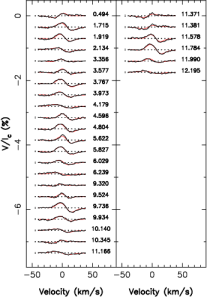
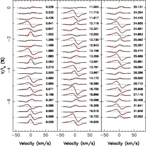
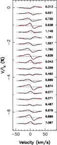
Figure 13: Observed (thick black line) and modelled (thin red line) LSD Stokes $V$ profiles of the photospheric lines of AU Mic, for seasons 2019 Sep-Nov (top left), 2020 Apr-Nov (bottom left), 2021 Jun-Nov (top right) and 2022 May-Jun (bottom right). The ZDI modeling of these profiles is described in Sec. 5.2. Rotation cycles (counting from $-53$, $-4$, 79 and 146 for 2019, 2020, 2021 and 2022 respectively, see Table 5) and $\pm$1$\sigma$ error bars are indicated to the right and left of each profile.

Appendix C Simulated Stokes $Q$ and $U$ LSD profiles

We present in Fig. 14 the simulated $Q$ and $U$ LSD profiles corresponding to our ZDI images of AU Mic for season 2020 Apr-Nov, shown in Figs. 4 and Figs. 5 and derived with the Stokes $V$ and Stokes $I$ & $V$ analyses detailed in Secs. 5.2 and 5.4. It shows in particular that Stokes $Q$ and $U$ observations of AU Mic can be used to distinguish between both magnetic configurations, whose Stokes $V$ signatures are similar.

Figure 14: Calculated LSD Stokes $Q$ (top panel) and $U$ (bottom panel) signatures associated with the reconstructed magnetic topologies of AU Mic for season 2020 Apr-Nov, derived with the Stokes $V$ (black line) and Stokes $I$ & $V$ (red line) analyses outlined in Secs. 5.2 and 5.3 and shown in Figs. 4 (second top row) and 5. Error bars to the left of each profile, depicting the achievable photon noise with exposure times listed in Table 5, demonstrate that such signatures are detectable and can be used to distinguish between both magnetic configurations, whose Stokes $V$ signatures are similar.

Appendix D The He i and Pa${\beta}$ line profiles of AU Mic

We show in Fig. 15 the spectra of AU Mic in the region of the He i triplet and Pa${\beta}$ line, in the stellar rest frame.

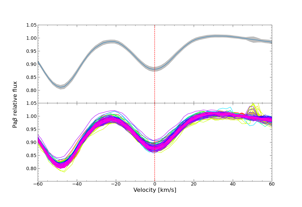
Figure 15: Spectra of AU Mic in the region of the He i triplet (top panel) and Pa${\beta}$ line (bottom panel), in the stellar rest frame. In each panel, the bottom curves show the superposition of individual spectra, whereas the top curve shows the median profile and dispersion (in grey shade). The red vertical dotted lines depict the location of the He i triplet end of the Pa${\beta}$ line.

Appendix E Stability and predicted TTVs of the planetary system

We show in Fig. 16 the stability of the planetary system in cases b+c+d and b+c+d+e, for a range of periods and eccentricities of candidate planet d. It confirms that b+c+d is stable for the 12.74-d period and low eccentricity orbit of planet d suggested by Wittrock et al. (2023), whereas b+c+d+e, though less stable, should still be able to survive on long timescales. Besides, we show in Fig. 17 the predicted TTVs for transiting planets b and c in the b+c+d+e and b+d+e cases, compared with the TESS, Spitzer and CHEOPS timing measurements.

Figure 16: Same as Fig. 12 for candidate planet d in the case of the b+c+d (top panel) and b+c+d+e (bottom panel) systems. In both cases, the system is stable for the 12.74-d period and low eccentricity orbit of candidate planet d suggested by Wittrock et al. (2023), though slightly less for the 4-planet than for the 3-planet system. The 3:2 resonances between d-b and c-d are strongest around $P_{d}\simeq 12.66$ d, with b+c+d being only stable for $e_{d}=$ 0.15–0.20 and b+c+d+e becoming unstable on a Gyr timescale.

Figure 17: Predicted TTVs for transiting planets b (top) and c (bottom), in the b+c+e (red line) and b+c+d+e (green line, with the mass of candidate planet d set to 0.68 ${\rm M}_{\oplus}$) cases, compared with the transit timings derived by TESS, Spitzer and CHEOPS (black open circles, Szabó et al., 2022).

References

- Afram & Berdyugina (2019) Afram N., Berdyugina S. V., 2019, A&A, 629, A83
- Alvarado-Gómez et al. (2022) Alvarado-Gómez J. D., et al., 2022, ApJ, 928, 147
- Artigau et al. (2022) Artigau É., et al., 2022, AJ, 164, 84
- Baraffe et al. (2015) Baraffe I., Homeier D., Allard F., Chabrier G., 2015, A&A, 577, A42
- Blinova et al. (2016) Blinova A. A., Romanova M. M., Lovelace R. V. E., 2016, MNRAS, 459, 2354
- Boccaletti et al. (2015) Boccaletti A., et al., 2015, Nature, 526, 230
- Boccaletti et al. (2018) Boccaletti A., et al., 2018, A&A, 614, A52
- Cale et al. (2021) Cale B. L., et al., 2021, AJ, 162, 295
- Carmona et al. (2023) Carmona A., et al., 2023, arXiv e-prints, p. arXiv:2303.16712
- Carolan et al. (2020) Carolan S., Vidotto A. A., Plavchan P., Villarreal D’Angelo C., Hazra G., 2020, MNRAS, 498, L53
- Chabrier et al. (2007) Chabrier G., Gallardo J., Baraffe I., 2007, A&A, 472, L17
- Chib & Jeliazkov (2001) Chib S., Jeliazkov I., 2001, Journal of the American Statistical Association, 96, 270
- Cifuentes et al. (2020) Cifuentes C., et al., 2020, A&A, 642, A115
- Cook et al. (2022) Cook N. J., et al., 2022, PASP, 134, 114509
- Correia et al. (2010) Correia A. C. M., et al., 2010, A&A, 511, A21
- Cristofari et al. (2022a) Cristofari P. I., et al., 2022a, MNRAS, 511, 1893
- Cristofari et al. (2022b) Cristofari P. I., et al., 2022b, MNRAS, 516, 3802
- Cristofari et al. (2023) Cristofari P. I., et al., 2023, MNRAS,
- Cutri et al. (2003) Cutri R. M., et al., 2003, VizieR Online Data Catalog, p. II/246
- David et al. (2019) David T. J., Petigura E. A., Luger R., Foreman-Mackey D., Livingston J. H., Mamajek E. E., Hillenbrand L. A., 2019, ApJ, 885, L12
- Delchambre (2015) Delchambre L., 2015, MNRAS, 446, 3545
- Donati & Landstreet (2009) Donati J., Landstreet J. D., 2009, ARA&A, 47, 333
- Donati et al. (1997) Donati J.-F., Semel M., Carter B. D., Rees D. E., Collier Cameron A., 1997, MNRAS, 291, 658
- Donati et al. (2003) Donati J.-F., Collier Cameron A., Petit P., 2003, MNRAS, 345, 1187
- Donati et al. (2006) Donati J.-F., et al., 2006, MNRAS, 370, 629
- Donati et al. (2020) Donati J. F., et al., 2020, MNRAS, 498, 5684
- Dotter et al. (2008) Dotter A., Chaboyer B., Jevremović D., Kostov V., Baron E., Ferguson J. W., 2008, ApJS, 178, 89
- Feiden (2016) Feiden G. A., 2016, A&A, 593, A99
- Finociety & Donati (2022) Finociety B., Donati J. F., 2022, MNRAS, 516, 5887
- Finociety et al. (2021) Finociety B., et al., 2021, MNRAS, 508, 3427
- Finociety et al. (2023) Finociety B., et al., 2023, MNRAS, 520, 3049
- Gaia Collaboration et al. (2021) Gaia Collaboration et al., 2021, A&A, 649, A1
- Gaidos et al. (2014) Gaidos E., et al., 2014, MNRAS, 443, 2561
- Gallenne et al. (2022) Gallenne A., Desgrange C., Milli J., Sanchez-Bermudez J., Chauvin G., Kraus S., Girard J. H., Boccaletti A., 2022, A&A, 665, A41
- García Muñoz et al. (2021) García Muñoz A., Fossati L., Youngblood A., Nettelmann N., Gandolfi D., Cabrera J., Rauer H., 2021, ApJ, 907, L36
- Haywood et al. (2014) Haywood R. D., et al., 2014, MNRAS, 443, 2517
- Haywood et al. (2022) Haywood R. D., et al., 2022, ApJ, 935, 6
- Hébrard et al. (2016) Hébrard É. M., Donati J. F., Delfosse X., Morin J., Moutou C., Boisse I., 2016, MNRAS, 461, 1465
- Hirano et al. (2020) Hirano T., et al., 2020, ApJ, 899, L13
- Ibañez Bustos et al. (2019) Ibañez Bustos R. V., Buccino A. P., Flores M., Martinez C. I., Maizel D., Messina S., Mauas P. J. D., 2019, MNRAS, 483, 1159
- Kalas et al. (2004) Kalas P., Liu M. C., Matthews B. C., 2004, Science, 303, 1990
- Kavanagh et al. (2021) Kavanagh R. D., Vidotto A. A., Klein B., Jardine M. M., Donati J.-F., Ó Fionnagáin D., 2021, MNRAS, 504, 1511
- Kiraga (2012) Kiraga M., 2012, Acta Astron., 62, 67
- Kislyakova et al. (2018) Kislyakova K. G., Fossati L., Johnstone C. P., Noack L., Lüftinger T., Zaitsev V. V., Lammer H., 2018, ApJ, 858, 105
- Klein et al. (2021) Klein B., et al., 2021, MNRAS, 502, 188
- Klein et al. (2022) Klein B., et al., 2022, MNRAS, 512, 5067
- Kochukhov (2021) Kochukhov O., 2021, A&ARv, 29, 1
- Kochukhov & Reiners (2020) Kochukhov O., Reiners A., 2020, ApJ, 902, 43
- Landi degl’Innocenti & Landolfi (2004) Landi degl’Innocenti E., Landolfi M., 2004, Polarisation in spectral lines. Dordrecht/Boston/London: Kluwer Academic Publishers
- Laskar (1993) Laskar J., 1993, Physica D Nonlinear Phenomena, 67, 257
- Laskar & Robutel (2001) Laskar J., Robutel P., 2001, Celestial Mechanics and Dynamical Astronomy, 80, 39
- Lehmann & Donati (2022) Lehmann L. T., Donati J. F., 2022, MNRAS, 514, 2333
- Leleu et al. (2021) Leleu A., et al., 2021, A&A, 649, A26
- López-Valdivia et al. (2021) López-Valdivia R., et al., 2021, ApJ, 921, 53
- Maldonado et al. (2020) Maldonado J., et al., 2020, A&A, 644, A68
- Malo et al. (2014) Malo L., Doyon R., Feiden G. A., Albert L., Lafrenière D., Artigau É., Gagné J., Riedel A., 2014, ApJ, 792, 37
- Mamajek & Bell (2014) Mamajek E. E., Bell C. P. M., 2014, MNRAS, 445, 2169
- Martioli et al. (2020) Martioli E., et al., 2020, A&A, 641, L1
- Martioli et al. (2021) Martioli E., Hébrard G., Correia A. C. M., Laskar J., Lecavelier des Etangs A., 2021, A&A, 649, A177
- Mesquita et al. (2022) Mesquita A. L., Rodgers-Lee D., Vidotto A. A., Kavanagh R. D., 2022, MNRAS, 515, 1218
- Miret-Roig et al. (2020) Miret-Roig N., et al., 2020, A&A, 642, A179
- Mishra et al. (2023) Mishra L., Alibert Y., Udry S., Mordasini C., 2023, A&A, 670, A68
- Morales et al. (2010) Morales J. C., Gallardo J., Ribas I., Jordi C., Baraffe I., Chabrier G., 2010, ApJ, 718, 502
- Morin et al. (2008a) Morin J., et al., 2008a, MNRAS, 384, 77
- Morin et al. (2008b) Morin J., et al., 2008b, MNRAS, 390, 567
- Morin et al. (2010) Morin J., Donati J., Petit P., Delfosse X., Forveille T., Jardine M. M., 2010, MNRAS, 407, 2269
- Morrell & Naylor (2019) Morrell S., Naylor T., 2019, MNRAS, 489, 2615
- Owen & Wu (2013) Owen J. E., Wu Y., 2013, ApJ, 775, 105
- Pecaut & Mamajek (2013) Pecaut M. J., Mamajek E. E., 2013, ApJS, 208, 9
- Perger et al. (2023) Perger M., et al., 2023, arXiv e-prints, p. arXiv:2301.12872
- Plavchan et al. (2020) Plavchan P., et al., 2020, Nature, 582, 497
- Reiners et al. (2022) Reiners A., et al., 2022, A&A, 662, A41
- Ryabchikova et al. (2015) Ryabchikova T., Piskunov N., Kurucz R. L., Stempels H. C., Heiter U., Pakhomov Y., Barklem P. S., 2015, Phys. Scr., 90, 054005
- Siess et al. (2000) Siess L., Dufour E., Forestini M., 2000, A&A, 358, 593
- Skilling & Bryan (1984) Skilling J., Bryan R. K., 1984, MNRAS, 211, 111
- Strugarek et al. (2015) Strugarek A., Brun A. S., Matt S. P., Réville V., 2015, ApJ, 815, 111
- Suárez Mascareño et al. (2020) Suárez Mascareño A., et al., 2020, A&A, 639, A77
- Suárez Mascareño et al. (2021) Suárez Mascareño A., et al., 2021, Nature Astronomy, 6, 232
- Szabó et al. (2021) Szabó G. M., et al., 2021, A&A, 654, A159
- Szabó et al. (2022) Szabó G. M., et al., 2022, A&A, 659, L7
- Van Eylen et al. (2019) Van Eylen V., et al., 2019, AJ, 157, 61
- Wittrock et al. (2023) Wittrock J. M., et al., 2023, arXiv e-prints, p. arXiv:2302.04922
- Zanni & Ferreira (2013) Zanni C., Ferreira J., 2013, A&A, 550, A99
- Zeng et al. (2016) Zeng L., Sasselov D. D., Jacobsen S. B., 2016, ApJ, 819, 127
- Zeng et al. (2019) Zeng L., et al., 2019, Proceedings of the National Academy of Science, 116, 9723
- Zicher et al. (2022) Zicher N., et al., 2022, MNRAS, 512, 3060