Positive flow-spines and contact $3$-manifolds, II

Abstract.

This paper corresponds to Section 8 of arXiv:1912.05774v3 [math.GT]. The contents until Section 7 are published in Annali di Matematica Pura ed Applicata as a separate paper. In that paper, it is proved that for any positive flow-spine $P$ of a closed, oriented $3$-manifold $M$, there exists a unique contact structure supported by $P$ up to isotopy. In particular, this defines a map from the set of isotopy classes of positive flow-spines of $M$ to the set of isotopy classes of contact structures on $M$. In this paper, we show that this map is surjective. As a corollary, we show that any flow-spine can be deformed to a positive flow-spine by applying first and second regular moves successively.

1. Introduction

In [10], closed, connected, oriented, contact $3$-manifolds are related to $2$-dimensional simple polyhedra with specific structure, called positive flow-spines. A non-singular flow $\mathcal{F}$ in a closed, connected, oriented, $3$-manifold $M$ is said to be carried by a flow-spine $P$ of $M$ if $\mathcal{F}$ is transverse to $P$ and is a “constant flow” in the complement of $P$ in $M$. A contact structure $\xi$ on $M$ is said to be supported by a flow-spine $P$ if there exists a contact form $\alpha$ on $M$ such that $\xi=\ker\alpha$ and its Reeb flow is carried by $P$. A flow-spine has two types of vertices: the vertex on the left in Figure 1 is said to be of $\ell$-type and the one on the right is of $r$-type. A flow-spine is then said to be positive if it has at least one vertex and all vertices are of $\ell$-type. It is proved in [10] that for any positive flow-spine $P$ of a closed, oriented $3$-manifold $M$, there exists a unique contact structure supported by $P$ up to isotopy. This defines a map from the set of isotopy classes of positive flow-spines of $M$ to the set of isotopy classes of contact structures on $M$. The following main theorem of the present paper shows that this map is surjective.

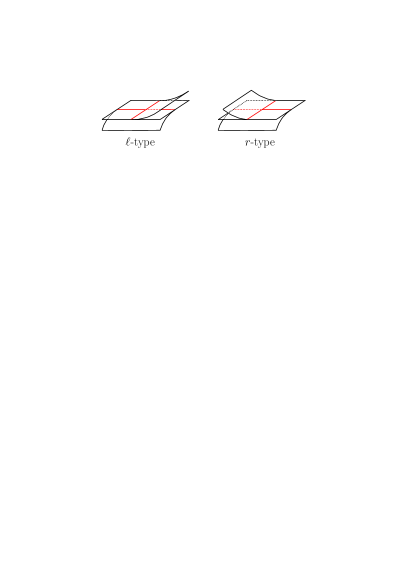
Figure 1. Vertices of $\ell$-type and $r$-type. Here, the ambient space is equipped with the right-handed orientation.

Theorem 1.1.

For any closed, connected, oriented, contact $3$-manifold $(M,\xi)$, there exists a positive flow-spine $P$ of $M$ that supports $\xi$.

As mentioned above, this theorem gives a surjection from the set of isotopy classes of positive flow-spines of $M$ to the set of isotopy classes of contact structures on $M$. It also gives a surjection from the set of positive flow-spines up to homeomorphism to the set of contact $3$-manifolds up to contactomorphism. To get a one-to-one correspondence, we need to find suitable moves of positive flow-spines. Moves of flow-spines are known in [9, 1, 3]. However, moves of positive flow-spines are very rare since most known moves for flow-spines yield $r$-type vertices. Theorem 1.1 implies that any flow-spine can be deformed to a positive one by regular moves, see Corollary 3.3.

The surjection from the set of positive flow-spines up to homeomorphism to the set of contact $3$-manifolds up to contactomorphism allows us to define a complexity for contact $3$-manifolds like the Matveev complexity for usual $3$-manifolds. This will be discussed in a forthcoming paper.

In Section 2, we briefly introduce fundamental notions such as contact $3$-manifolds, branched polyhedra, flow-spines, regular moves and the construction of a contact form from a positive flow-spine used in [10]. The proof of Theorem 1.1 is given in Section 3.

The second author is supported by JSPS KAKENHI Grant Numbers JP19K03499 and JSPS-VAST Joint Research Program, Grant number JPJSBP120219602. The third author is supported by JSPS KAKENHI Grant Numbers JP20K03588 and JP21H00978. The fourth author is supported by JSPS KAKENHI Grant Numbers JP19K21019 and 20K14316.

2. Preliminaries

Throughout this paper, for a polyhedral space $X$, $\mathrm{Int\,}X$ represents the interior of $X$, $\partial X$ represents the boundary of $X$, and $\mathrm{Nbd}(Y;X)$ represents a closed regular neighborhood of a subspace $Y$ of $X$ in $X$, where $X$ is equipped with the natural PL structure if $X$ is a smooth manifold. The set $\mathrm{Int\,}\mathrm{Nbd}(Y;X)$ is the interior of $\mathrm{Nbd}(Y;X)$ in $X$.

2.1. Contact $3$-manifolds

In this subsection, we briefly recall notions and known results in $3$-dimensional contact topology that will be used in this paper. The reader may find general explanation, for instance, in [4, 5, 14].

Let $M$ be a closed, oriented, smooth $3$-manifold. A contact structure on $M$ is the $2$-plane field on $M$ given by the kernel of a $1$-form $\alpha$ on $M$ satisfying $\alpha\land d\alpha\neq 0$ everywhere. The $1$-form $\alpha$ is called a contact form. If $\alpha\land d\alpha>0$ everywhere on $M$ then the contact structure given by $\ker\alpha$ is called a positive contact structure and the $1$-form $\alpha$ is called a positive contact form. The pair of a closed, oriented, smooth $3$-manifold $M$ and a contact structure $\xi=\ker\alpha$ on $M$ is called a contact $3$-manifold and denoted by $(M,\xi)$. In this paper, by a contact structure we mean a positive one.

Two contact structures $\xi$ and $\xi^{\prime}$ on $M$ are said to be isotopic if there exists a one-parameter family of contact forms $\alpha_{t}$, $t\in[0,1]$, such that $\xi=\ker\alpha_{0}$ and $\xi^{\prime}=\ker\alpha_{1}$. Two contact $3$-manifolds $(M,\xi)$ and $(M^{\prime},\xi^{\prime})$ are said to be contactomorphic if there exists a diffeomorphism $\phi:M\to M^{\prime}$ such that $\phi_{*}(\xi)=\xi^{\prime}$. The map $\phi$ is called a contactomorphism. If $M=M^{\prime}$ then we also say that $\xi$ and $\xi^{\prime}$ are contactomorphic. The Gray theorem states that if two contact structures are isotopic then they are contactomorphic [7].

Next we introduce the Reeb vector field. Let $\alpha$ be a contact form on $M$. A vector field $X$ on $M$ determined by the conditions $d\alpha(X,\cdot)=0$ and $\alpha(X)=1$ is called the Reeb vector field of $\alpha$ on $M$. Such a vector field is uniquely determined by $\alpha$ and we denote it by $R_{\alpha}$. The non-singular flow on a $3$-manifold $M$ generated by a Reeb vector field is called a Reeb flow.

The Reeb vector field plays important roles in many studies in contact geometry and topology. In $3$-dimensional contact topology, it is used to give a correspondence between contact structures and open book decompositions of $3$-manifolds. Let $\Sigma$ be an oriented, compact surface with boundary and $\phi:\Sigma\to\Sigma$ be a diffeomorphism such that $\phi|_{\partial\Sigma}$ is the identity map on $\partial\Sigma$. If a closed, oriented $3$-manifold $M$ is orientation-preservingly homeomorphic to the quotient space obtained from $\Sigma\times[0,1]$ by the identification $(x,1)\sim(\phi(x),0)$ for $x\in\Sigma$ and $(y,0)\sim(y,t)$ for each $y\in\partial\Sigma$ and any $t\in[0,1]$, then we say that it is an open book decomposition of $M$. The image $L$ of $\partial\Sigma$ in $M$ by the quotient map is called the binding, which equips the orientation as the boundary of $\Sigma$. The image of the surface $\Sigma\times\{t\}$ in $M$ is called a page. We denote the open book by $(M,\Sigma,L,\phi)$.

A contact structure $\xi$ on $M$ is said to be supported by an open book $(M,\Sigma,L,\phi)$ if there exists a contact form $\alpha$ on $M$ such that $\xi=\ker\alpha$ and the Reeb vector field $R_{\alpha}$ of $\alpha$ satisfies that

• $R_{\alpha}$ is tangent to $L$ and the orientation on $L$ induced from $\Sigma$ coincides with the direction of $R_{\alpha}$, and

• $R_{\alpha}$ is positively transverse to $\mathrm{Int\,}\Sigma\times\{t\}$ for any $t\in[0,1]$.

Any open book has a supported contact structure and this is used by Thurston and Winkelnkemper to prove that any closed, oriented, smooth $3$-manifold admits a contact structure [16]. Note that the existence of a contact structure for any $3$-manifold was first proved by Martinet [12]. Giroux then showed that the contact structure supported by a given open book is unique up to isotopy [6]. He also proved the following theorem, that will be used in the proof of Theorem 1.1.

Theorem 2.1 (Giroux, cf. [4]).

For any contact $3$-manifold $(M,\xi)$, there exists an open book decomposition of $M$ that supports $\xi$.

These results of Giroux give a surjection from the set of isotopy classes of open book decompositions of $M$ to the set of isotopy classes of contact structures on $M$, and also a surjection from the set of open books up to homeomorphism to the set of contact $3$-manifolds up to contactomorphism. Taking the quotient of the set of open books of $M$ by a certain operation for pages of open books, called a stabilization, we can think one-to-one correspondence between open books and contact $3$-manifolds, that is called the Giroux correspondence.

2.2. Branched polyhedron

A compact topological space $P$ is called a simple polyhedron, or a quasi-standard polyhedron, if every point of $P$ has a regular neighborhood homeomorphic to one of the three local models shown in Figure 2. A point whose regular neighborhood is shaped on the model (iii) is called a true vertex of $P$ (or vertex for short), and we denote the set of true vertices of $P$ by $V(P)$. The set of points whose regular neighborhoods are shaped on the models (ii), (iii) and (v) is called the singular set of $P$, and we denote it by $S(P)$. The set of points whose regular neighborhoods are shaped on the models (iv) and (v) is called the boundary of $P$, and we denote it by $\partial P$. Each connected component of $P\setminus S(P)$ is called a region of $P$ and each connected component of $S(P)\setminus V(P)$ is called an edge of $P$. A simple polyhedron $P$ is said to be special, or standard, if each region of $P$ is an open disk and each edge of $P$ is an open arc. Throughout this paper, we assume that all regions are orientable.

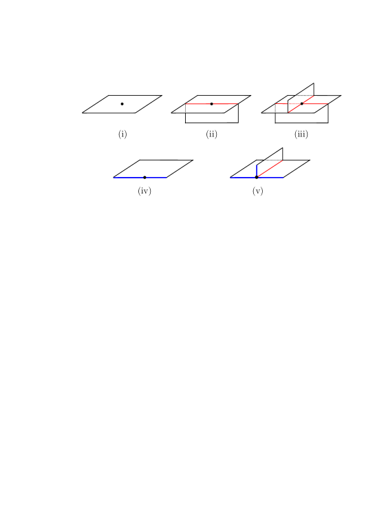
Figure 2. The local models of a simple polyhedron.

A branching of a simple polyhedron $P$ is an assignment of orientations to regions of $P$ such that the three orientations on each edge of $P$ induced by the three adjacent regions do not agree. We note that even though each region of a simple polyhedron $P$ is orientable, $P$ does not necessarily admit a branching. See [8, 1, 11, 15] for general properties of branched polyhedra.

2.3. Flow-spines

A polyhedron $P$ is called a spine of a closed, connected, oriented $3$-manifold $M$ if it is embedded in $M$ and $M$ with removing an open ball collapses onto $P$. If a spine is simple then it is called a simple spine.

If a simple spine $P$ admits a branching, then it allows us to smoothen $P$ in the ambient manifold $M$ as in the local models shown in Figure 3. A point of $P$ whose regular neighborhood is shaped on the model (iii) is called a vertex of $\ell$-type and that on the model (iv) is a vertex of $r$-type.

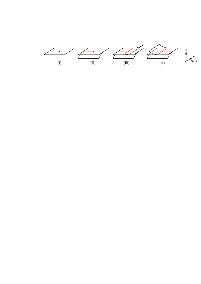
Figure 3. The local models of a branched simple polyhedron.

Definition.

Let $M$ be a closed, connected, oriented $3$-manifold.

• Let $(M,\mathcal{F})$ be a pair of $M$ and a non-singular flow $\mathcal{F}$ on $M$. A simple spine $P$ of $M$ is called a flow-spine of $(M,\mathcal{F})$ if, for each point $p\in P$, there exists a positive coordinate chart $(U;x,y,z)$ of $M$ around $p$ such that $(U,p)$ is one of the models in Figure 3, where $\mathcal{F}|_{U}$ is generated by $\frac{\partial}{\partial z}$, and $\mathcal{F}|_{M\setminus P}$ is a constant vertical flow shown in Figure 4.

• A branched simple spine $P$ of $M$ is called a flow-spine of $M$ if it is a flow-spine of $(M,\mathcal{F})$ for some non-singular flow $\mathcal{F}$ on $M$. The flow $\mathcal{F}$ is said to be carried by $P$.

Figure 4. The flow in the complement $M\setminus P$.

2.4. Regular moves

In this subsection, we introduce two kinds of moves of branched simple polyhedra.

Definition.

• The moves shown in Figure 5 and their mirrors are called first regular moves [9] or Matveev-Piergallini moves [1].

• The moves shown in Figure 6 and their mirrors are called second regular moves [9] or lune moves [13].

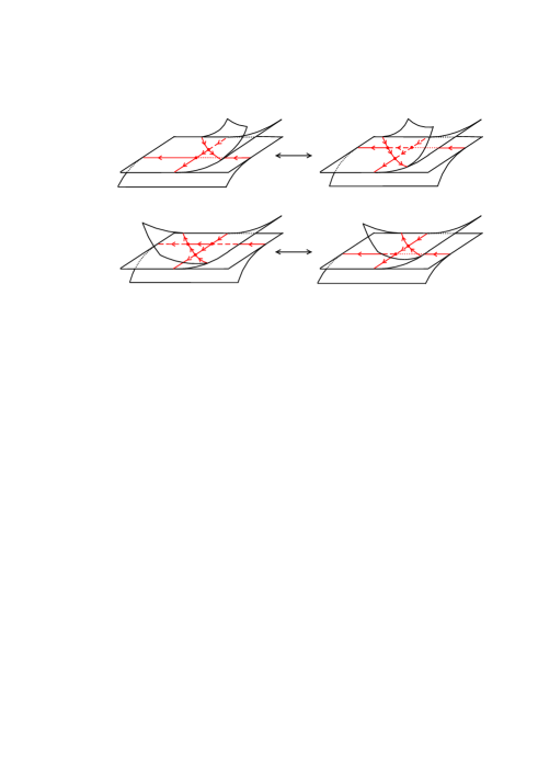
Figure 5. First regular moves.

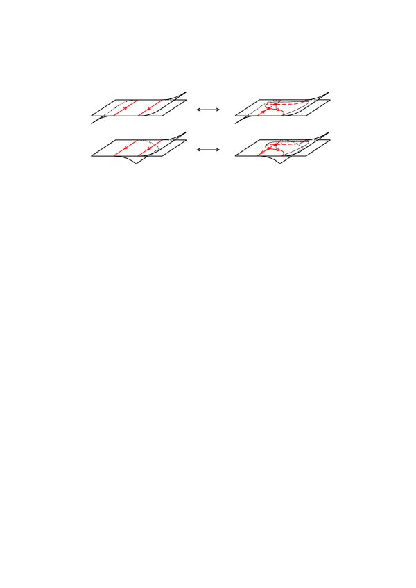
Figure 6. Second regular moves.

These moves are enough to trace deformation of non-singular flows in $3$-manifolds. Two non-singular flows $\mathcal{F}_{1}$ and $\mathcal{F}_{2}$ in a closed, orientable $3$-manifold are said to be homotopic if there exists a smooth deformation from $\mathcal{F}_{1}$ to $\mathcal{F}_{2}$ in the set of non-singular flows.

Theorem 2.2 ([9]).

Let $P_{1}$ and $P_{2}$ be flow-spines of a closed, orientable $3$-manifold $M$. Let $\mathcal{F}_{1}$ and $\mathcal{F}_{2}$ be flows on $M$ carried by $P_{1}$ and $P_{2}$, respectively. Suppose that $\mathcal{F}_{1}$ and $\mathcal{F}_{2}$ are homotopic. Then $P_{1}$ is obtained from $P_{2}$ by applying first and second regular moves successively.

2.5. Construction of a contact form from a positive flow-spine

In this subsection, we briefly recall the construction of a contact form on a closed, connected, oriented, smooth $3$-manifold $M$ from its positive flow-spine $P$ introduced in [10].

For a positive flow-spine $P$ of $M$, set $Q=\mathrm{Nbd}(S(P);P)$ and let $\mathcal{R}_{i}$ be the connected component of $P\setminus\mathrm{Int\,}Q$ contained in a region $R_{i}$ of $P$. Let $\mathrm{Nbd}(S(P);M)$ be a neighborhood of $S(P)$ in $M$, choose a neighborhood $N_{P}=\mathrm{Nbd}(P;M)$ of $P$ in $M$ sufficiently thin with respect to $\mathrm{Nbd}(S(P);M)$, and set $N_{Q}=\mathrm{Nbd}(P;M)\cap\mathrm{Nbd}(S(P);M)$. Then $M$ decomposes as

$$M=N_{P}\cup N_{D}=\left(N_{Q}\cup\bigcup_{i=1}^{n}N_{\mathcal{R}_{i}}\right)\cup N_{D},$$

where $N_{\mathcal{R}_{i}}$ is the connected component of the closure of $N_{P}\setminus N_{Q}$ containing $\mathcal{R}_{i}$, which is diffeomorphic to $\mathcal{R}_{i}\times[0,1]$, and $N_{D}$ is the closure of $M\setminus N_{P}$, which is a $3$-ball. The boundary of $N_{P}$ consists of “vertical part” and “horizontal part”. The “vertical part” is the vertical face of $N_{P}$ shown on the right in Figure 7, which constitutes an annulus. The union of the rest faces of $N_{P}$ is the “horizontal part”. We regard $N_{D}$ as $D^{2}\times[0,1]$, where $D^{2}$ is the unit $2$-disk, so that $\partial D^{2}\times[0,1]$ corresponds to the “vertical part” of $\partial N_{P}$.

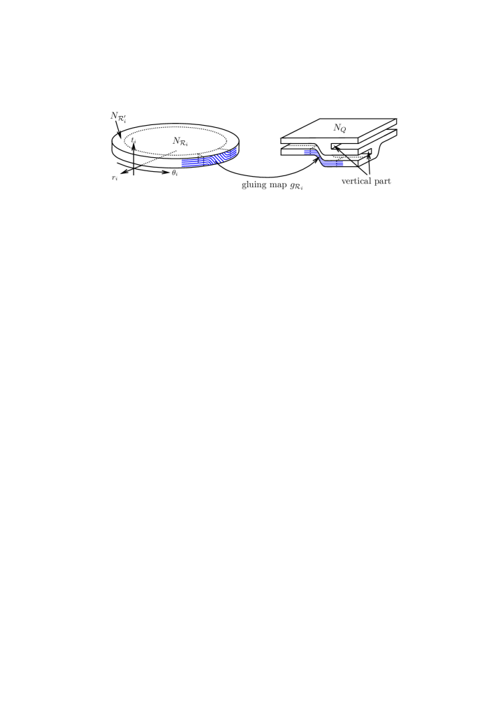
Figure 7. Construction of $N_{P}$.

A $1$-form $\eta$ on $M$ constructed in [10, Section 5], called a reference $1$-form, satisfies that

• $\eta\land d\eta\geq 0$ on $M$ and

• $d\eta=0$ on $N_{D}\setminus(\hat{W}\cup\check{W})$.

Property (a) is proved in [10, Lemma 5.8]. Property (b) follows from Lemma 5.6 (1), (2) and equation (5.4) in [10]. We omit the definition of $\hat{W}\cup\check{W}$. This part appears in small neighborhoods of the orbits of the flow passing though the vertices of $P$, cf. [10, Fig. 18], and we only use this fact in the proof of Theorem 1.1.

The next step is to construct a $1$-form $\beta$ on a positive flow-spine $P$ of $M$ such that $d\beta>0$. Let $\mathrm{pr}_{Q}:Q\to Q^{\prime}$ be a projection of $Q$ to an oriented, compact surface $Q^{\prime}$ such that, for each edge $e$ of $P$, the two adjacent regions of $Q$ that induce the same orientation to $e$ are identified. Note that $Q^{\prime}$ is homotopy equivalent to $S(P)$. A $1$-form on $P$ means that it is obtained by gluing the pullback of a $1$-form on $Q^{\prime}$ by the projection $\mathrm{pr}_{Q}:Q\to Q^{\prime}$ and $1$-forms on the regions $R_{1},\ldots,R_{n}$ of $P$. The existence of a $1$-form $\beta$ on $P$ with $d\beta>0$ is proved in [10, Lemma 6.3].

From this $\beta$, we make a $1$-form $\hat{\beta}$ on $N_{P}$. Let $\mathrm{pr}_{\mathcal{R}_{i}}:N_{\mathcal{R}_{i}}=\mathcal{R}_{i}\times[0,1]\to\mathcal{R}_{i}$ be the first projection and set $N_{\mathcal{R}_{i}^{\prime}}=\mathrm{Nbd}(\partial\mathcal{R}_{i};\mathcal{R}_{i})\times[0,1]\subset\mathcal{R}_{i}\times[0,1]$. Let $g_{\mathcal{R}_{i}}:N_{\mathcal{R}_{i}^{\prime}}\to N_{Q}$ be a gluing map of $N_{\mathcal{R}_{i}}$ to $N_{Q}$. Choose coordinates $(r_{i},\theta_{i})$ on $\mathrm{Nbd}(\partial\mathcal{R}_{i};\mathcal{R}_{i})$ so that $\{r_{i}=0\}=\partial\mathrm{Nbd}(\partial\mathcal{R}_{i};\mathcal{R}_{i})\setminus\partial\mathcal{R}_{i}$, $\{r_{i}=1\}=\partial\mathcal{R}_{i}$ and the orientation of $(r_{i},\theta_{i})$ coincides with that of $\mathcal{R}_{i}$, see the left in Figure 7. Let $\mathrm{pr}_{N_{Q}}:N_{Q}\to Q$ be a canonical projection. From the $1$-form $\beta$ on $P$, we define the $1$-form $\hat{\beta}$ on $N_{P}$ by gluing $\mathrm{pr}_{N_{Q}}^{*}\beta$ on $N_{Q}\setminus\bigcup_{i=1}^{n}g_{\mathcal{R}_{i}}(N_{\mathcal{R}^{\prime}_{i}})$ and

$$(1-\sigma(r_{i}))\mathrm{pr}_{\mathcal{R}_{i}}^{*}\beta+\sigma(r_{i})(\mathrm{pr}_{N_{Q}}\circ g_{\mathcal{R}_{i}})^{*}\beta$$

on $N_{\mathcal{R}_{i}}$, where $\sigma(r_{i})$ is a monotone increasing smooth function such that $\sigma(\varepsilon)=0$ and $\sigma(1-\varepsilon)=1$ for any sufficiently small $\varepsilon\geq 0$. It is verified in [10, Lemma 6.6] that $\hat{\beta}+R\eta$ is a contact form on $N_{P}$ whose Reeb vector field is positively transverse to $P$ for any $R>0$.

Next we extend the $1$-form $\hat{\beta}$ to $N_{D}=D^{2}\times[0,1]$. We extend the coordinate $[0,1]$ slightly and set $N_{D}^{\varepsilon}=D^{2}\times[-\varepsilon,1+\varepsilon]$ for a sufficiently small $\varepsilon>0$. Let $\hat{\beta}_{E}$ and $\hat{\beta}_{F}$ be the $1$-form $\hat{\beta}$ on $D^{2}\times[-\varepsilon,0]$ and $D^{2}\times[1,1+\varepsilon]$, respectively. Fix coordinates $(u,v,w)$ on $N_{D}^{\varepsilon}$ so that the $1$-forms $\hat{\beta}_{E}$ and $\hat{\beta}_{F}$ are invariant on their defining domains under translation to the $w$-coordinate. We then extend these forms to the whole $N_{D}$ canonically and denote them again by $\hat{\beta}_{E}$ and $\hat{\beta}_{F}$. Now we define a $1$-form $\hat{\beta}_{M}$ on $M$ by extending $\hat{\beta}$ on $N_{P}$ to $N_{D}=D^{2}\times[0,1]$ as

$$\hat{\beta}_{M}=(1-\tau(w))\hat{\beta}_{E}+\tau(w)\hat{\beta}_{F},$$

where $\tau:[-\varepsilon,1+\varepsilon]\to[0,1]$ is a monotone increasing smooth function such that $\tau(w)=0$ for $-\varepsilon\leq w\leq 0$ and $\tau(w)=1$ for $1\leq w\leq 1+\varepsilon$. The contact form on $M$ asserted in [10, Theorem 1.1] is given as $\hat{\beta}_{M}+R\eta$ for a sufficiently large $R>0$.

3. Proof of Theorem 1.1

In this section, we give the proof of Theorem 1.1.

Definition.

A vector field $Z$ on $M$ is called a monodromy vector field of an open book $(M,\Sigma,L,\phi)$ if

• $Z$ is tangent to the binding $L$ and the orientation on $L$ induced from $\Sigma$ coincides with the direction of $Z$, and

• $Z$ is positively transverse to $\mathrm{Int\,}\Sigma\times\{t\}$ for any $t\in[0,1]$.

In particular, the Reeb vector field used in the definition of the contact structure supported by an open book in Section 2.1 is a monodromy vector field of the open book.

We first prove the following proposition.

Proposition 3.1.

Let $(M,\Sigma,L,\phi)$ be an open book decomposition of a closed, connected, oriented $3$-manifold $M$ whose page is a surface of genus at least $2$ and whose binding is connected. Then there exists a positive flow-spine on $M$ that carries the flow generated by a monodromy vector field of the open book.

Proof.

Let $g$ be the genus of $\Sigma$ and $a_{1},\ldots,a_{g}$, $b_{1},\ldots,b_{g-1}$, $c_{1},\ldots,c_{g}$ be the simple closed curves on the page as in Figure 8. Let $\sigma_{a_{i}}$, $\sigma_{b_{i}}$ and $\sigma_{c_{i}}$ denote the right-handed Dehn twists along $a_{i}$, $b_{i}$ and $c_{i}$, respectively.

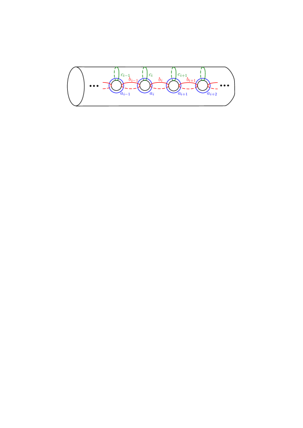
Figure 8. Curves for Dehn twists.

We represent the monodromy of the open book by a product of Dehn twists as $w_{1}^{m_{1}}w_{2}^{m_{2}}\cdots w_{n}^{m_{n}}$, where $w_{k}$ is the Dehn twist along one of the curves $a_{1},\ldots,a_{g}$, $b_{1},\ldots,b_{g-1}$, $c_{1},\ldots,c_{g}$. Here we read the product from left to right. Let $f:M\setminus\mathrm{Int\,}\mathrm{Nbd}(L;M)\to S^{1}$ be a smooth non-singular map of the open book. Choose $6n$ points $q_{1},\ldots,q_{6n}$ on $S^{1}$ in the counter-clockwise order and set $\Sigma_{j}=f^{-1}(q_{j})$. We assign to each $\Sigma_{j}$ the orientation as a page of the open book.

We first draw a graph, which will become $S(P)$, on each $\Sigma_{j}$ as shown in Figures 9, 10, 11, 12, 13 and 14, depending on $j$ modulo $6$.

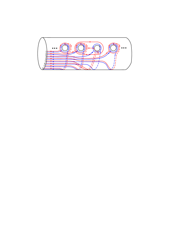
Figure 9. The singular set $S(P)$ on $\Sigma_{6k}$.

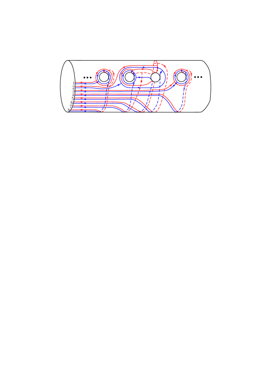
Figure 10. The singular set $S(P)$ on $\Sigma_{6k+1}$.

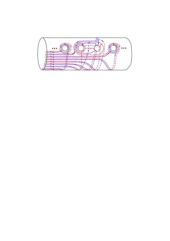
Figure 11. The singular set $S(P)$ on $\Sigma_{6k+2}$.

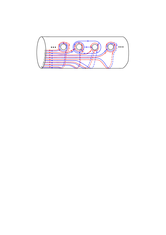
Figure 12. The singular set $S(P)$ on $\Sigma_{6k+3}$.

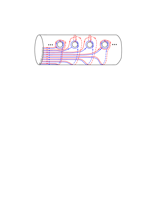
Figure 13. The singular set $S(P)$ on $\Sigma_{6k+4}$.

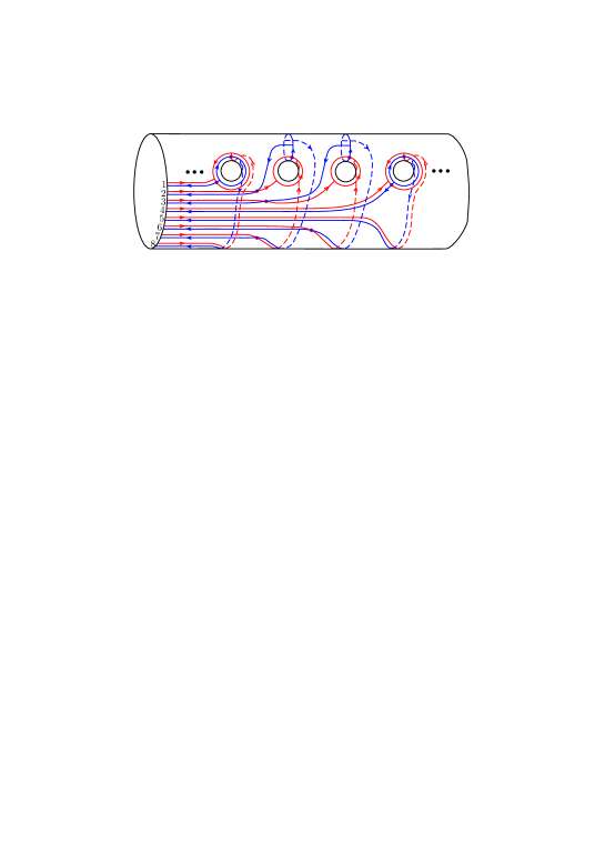
Figure 14. The singular set $S(P)$ on $\Sigma_{6k+5}$.

For each $j=1,\ldots,6n$, the red graph $G_{j}^{red}$ on $\Sigma_{j}$ and the blue graph $G_{j}^{blue}$ on $\Sigma_{j+1}$ coincide as unoriented graphs up to isotopy, which we denote by $G_{j}$, and their orientations are opposite. Here we regard $\Sigma_{6n+1}=\Sigma_{1}$. We attach $G_{j}\times[0,1]$ between $\Sigma_{j}$ and $\Sigma_{j+1}$ such that $G_{j}\times\{0\}=G_{j}^{red}$ and $G_{j}\times\{1\}=G_{j}^{blue}$. To each region of $G_{j}\times[0,1]$ we assign an orientation so that the induced orientation on the boundary coincides with those of the edges of $G_{j}^{red}$ and $G_{j}^{blue}$. See Figure 15 for the orientations on $G_{j}\times[0,1]$. A vertex of this branched polyhedron can be seen as either an intersection of a red edge and a blue edge on $\Sigma_{j}$ or a trivalent vertex on $\Sigma_{j}$. Any vertex in the former case is of $\ell$-type since the blue edge intersects the red one from the left to the right with respect to the orientation of the red edge. Other vertices are those appearing in Figure 15 and we can verify that they are of $\ell$-type in the figure directly.

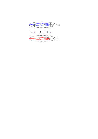
Figure 15. Attach $G_{j}\times[0,1]$. Black arrows in the figure show the smooth directions of the immersion of $S(P)$ at the vertices.

If $w_{k}=\sigma_{a_{p}}^{m_{p}}$ then we modify the $p$-th blue circle on $\Sigma_{6k+1}$ as shown on the left in Figure 16 if $m_{p}>0$ and as shown on the right if $m_{p}<0$. We may verify that all vertices appearing by this modification are of $\ell$-type.

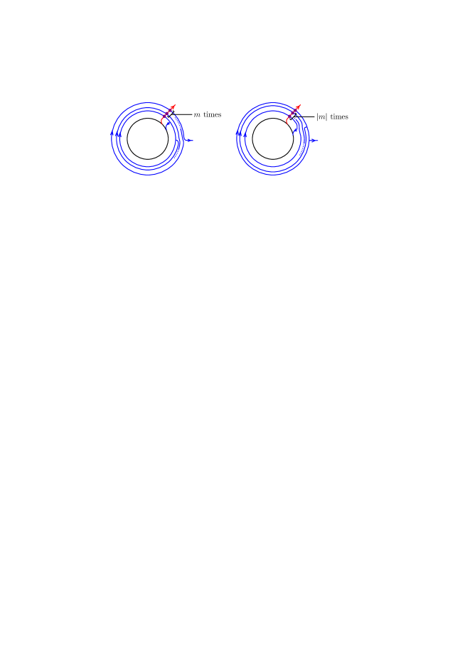
Figure 16. Modification of the polyhedron according to the Dehn twists $\sigma_{a_{p}}^{m_{p}}$.

If $w_{k}=\sigma_{b_{p}}^{m_{p}}$ then, we apply the same modification to the blue curve on $\Sigma_{6k+2}$ shown on the left in Figure 17, and if $w_{k}=\sigma_{c_{p}}^{m_{p}}$ then we do the same modification to the blue curve on $\Sigma_{6k+5}$ shown on the right. All vertices appearing by these modifications are also of $\ell$-type.

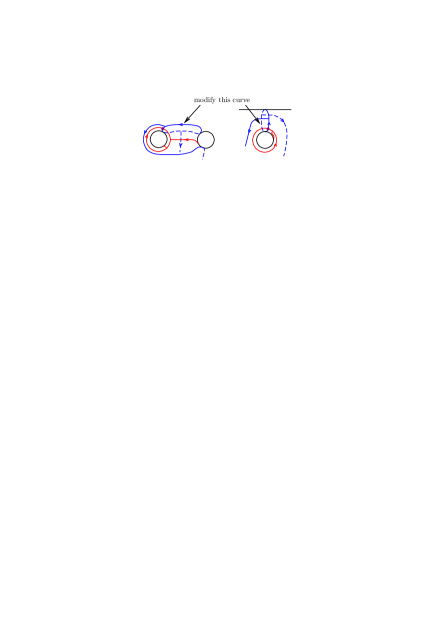
Figure 17. Curves for modifications corresponding to the Dehn twists $\sigma_{b_{p}}^{m_{p}}$ and $\sigma_{c_{p}}^{m_{p}}$.

We may choose a monodromy vector field of the open book on $M\setminus\mathrm{Int\,}\mathrm{Nbd}(L;M)$ such that it is positively transverse to the branched polyhedron constructed above. We denote the obtained branched polyhedron embedded in $M\setminus\mathrm{Int\,}\mathrm{Nbd}(L;M)$ by $\hat{P}_{1}$.

Next, we construct a branched polyhedron in $\mathrm{Nbd}(L;M)$. For each $(i,j)$, $i=1,\ldots,2g$, $j=1,\ldots,6n$, we set a polyhedron $P_{i,j}$ shown in Figure 18. Glue the left side of $P_{i,j}$ and the right side of $P_{i+1,j}$ canonically, where we regard $P_{2g+1,j}$ as $P_{1,j}$, and denote the obtained polyhedron by $P_{j}$ for $j=1,\ldots,6n$. We then glue $P_{j}$ and $P_{j+1}$ so that the top of $P_{i,j}$ is identified with the bottom of $P_{i,j+1}$, where $P_{6n+1}$ is regarded as $P_{1}$. We denote the obtained polyhedron by $\hat{P}_{2}$. We assign orientations to the regions of $\hat{P}_{2}$ as shown in Figure 18, so that $\hat{P}_{2}$ is a branched polyhedron. The boundary of $\hat{P}_{2}$ consists of $2g$ circles and a connected graph. Attach a disk $D_{i}$ to each of $2g$ circles and denote the obtained branched polyhedron by $\hat{P}_{3}$. We can embed $\hat{P}_{3}$ into the solid torus $D^{2}\times S^{1}$ properly. We regard this $D^{2}\times S^{1}$ as $\mathrm{Nbd}(L;M)$ and glue $\hat{P}_{3}$ and $\hat{P}_{1}$ so that the simple closed curve on $\partial\hat{P}_{3}\cap P_{j}$ (green curve) coincides with the boundary of $\Sigma_{j}$ in $\hat{P}_{1}$. We denote the obtained branched polyhedron embedded in $M$ by $\hat{P}_{4}$. We can easily check that all vertices of $\hat{P}_{4}$ are of $\ell$-type.

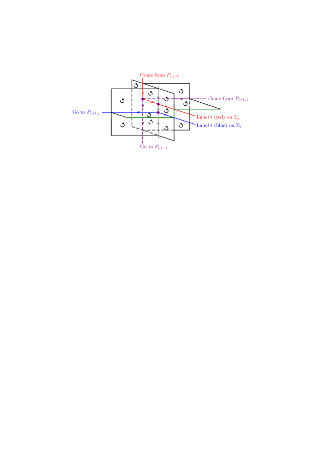
Figure 18. The piece $P_{i,j}$.

The complement $M\setminus\hat{P}_{4}$ consists of $2g+6n$ open balls $B_{1},\ldots,B_{2g}$ and $B^{\prime}_{1},\ldots,B^{\prime}_{6n}$, where the $2g$ balls $B_{1},\ldots,B_{2g}$ are the components bounded by $\hat{P}_{3}$ and each $B^{\prime}_{j}$, $j=1,\ldots,6n$, is the component of $M\setminus\hat{P}_{4}$ containing the connected component of $M\setminus\left(\hat{P}_{4}\cup\mathrm{Nbd}(L;M)\right)$ between $\Sigma_{j}$ and $\Sigma_{j+1}$.

The singular set $S(P)$ consists of $2g+6n$ immersed circles $C_{1},\ldots,C_{2g}$ and $C^{\prime}_{1},\ldots,C^{\prime}_{6n}$, where $C_{i}$ is a simple closed curve passing through $P_{i,1},\ldots,P_{1,6n}$, which is drawn in gray in Figure 18, and $C_{j}^{\prime}$ is a simple closed curve given as follows: Start from Label $1$ (red) on $\Sigma_{6k}$ in Figure 9 and follow the arrow. Let $P_{i_{0},6k}$ be the piece of $\hat{P}_{4}$ that contains the starting point. The curve passes through $P_{i_{0},6k+1}$ as depicted with black arrows in Figure 15 and comes back to Label $1$ (blue) on $\Sigma_{6k+1}$. Then, as shown in Figure 18, it goes to Label $2$ on $\Sigma_{6k+1}$ and then goes down to Label $2$ (red) on $\Sigma_{6k}$. By the same observation, we see that it passes through Labels $1,2,\ldots,8$ (red) on $\Sigma_{6k}$ in this order. This curve goes further and finally comes back to Label $1$ (red) on $\Sigma_{6k}$. This is the curve $C_{1}^{\prime}$. By the same way, the curves $C^{\prime}_{j}$, $j=2,\ldots,6n$, are defined.

We modify a part of $C_{i}$ on $P_{i,1}$ for each $i=1,\ldots,2g$ as shown in Figure 19 and remove the bigon that appears by this move. This modification does not yield a new vertex, connects $B_{i}$ to $B^{\prime}_{1}$ and makes $C_{i}$ and $C_{1}^{\prime}$ to be one immersed circle. Applying this modification to each of $C_{1},\ldots,C_{2g}$, we obtain a branched polyhedron $\hat{P}_{5}$ with only vertices of $\ell$-type such that $M\setminus\hat{P}_{5}$ consists of $6n$ open balls $B^{\prime\prime}_{1},B_{2}^{\prime},\ldots,B^{\prime}_{6n}$ and $S(P)$ consists of $6n$ immersed circles $C^{\prime\prime}_{1},C_{2}^{\prime}\ldots,C^{\prime}_{n}$, where $B_{1}^{\prime\prime}$ is the open ball obtained by connecting $B_{1},\ldots,B_{2g}$ with $B_{1}^{\prime}$ and $C_{1}^{\prime\prime}$ is the immersed circle obtained by connecting $C_{1},\ldots,C_{2g}$ with $C_{1}^{\prime}$.

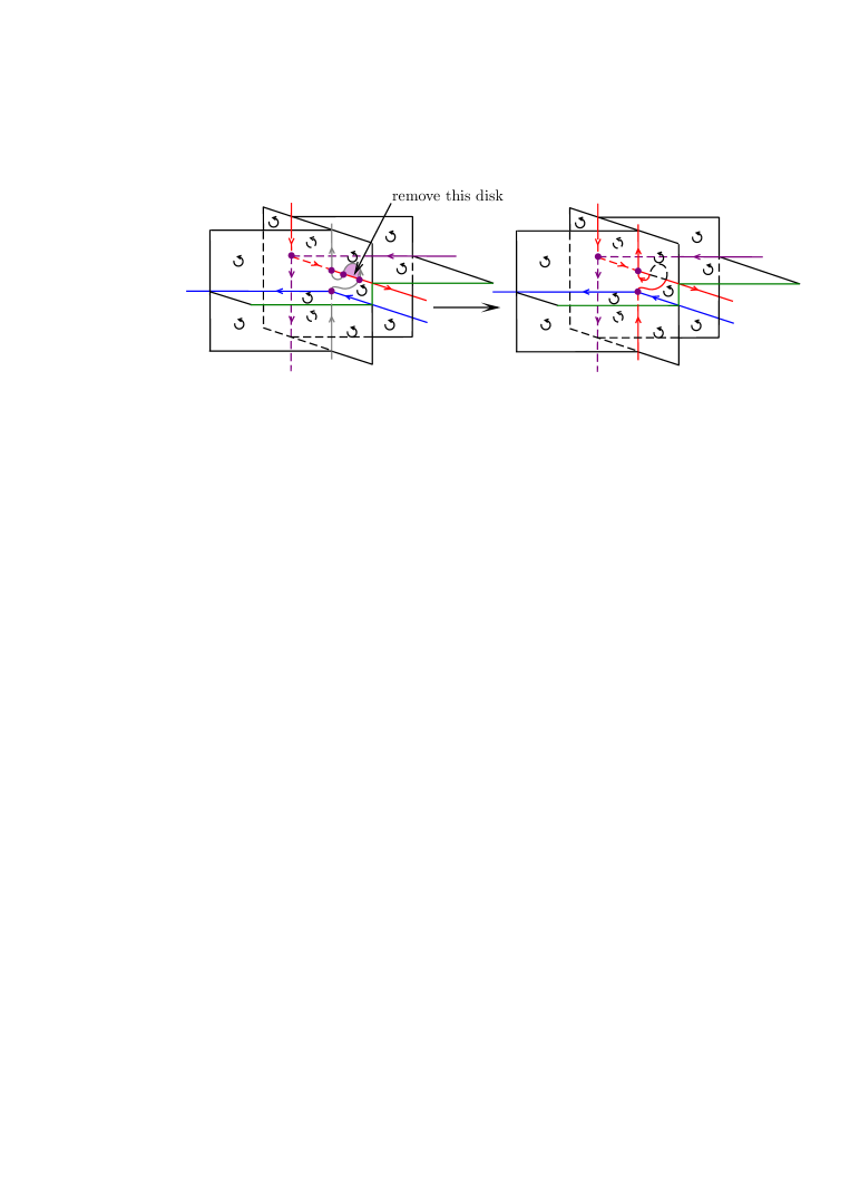
Figure 19. Modification of $C_{i}$ on $P_{i,j}$.

For each $j=2,\ldots,6n$, we apply the same modification to the same part of $C_{1}^{\prime\prime}$ on $P_{1,j}$. This does not yield a new vertex, connects $B^{\prime}_{j}$ to $B^{\prime\prime}_{1}$ and makes $C^{\prime\prime}_{1},C_{2}^{\prime},\ldots,C_{n}^{\prime}$ to be one immersed circle. The obtained branched polyhedron $\hat{P}_{6}$ satisfies that all vertices are of $\ell$-type, $M\setminus\hat{P}_{6}$ is one open ball and $S(P)$ is the image of an immersion of one circle.

We can see directly that there exists a monodromy vector field of the open book whose generated flow is carried by $\hat{P}_{6}$. Thus we obtain the assertion. ∎

To prove Theorem 1.1, we need to show the following stronger statement.

Proposition 3.2.

Let $(M,\Sigma,L,\phi)$ be an open book decomposition of a closed, connected, oriented $3$-manifold $M$ whose page is a surface of genus at least $2$ and whose binding is connected. Then there exists a positive flow-spine $P$ of $M$ and a contact form $\alpha$ on $M$ such that the Reeb flow is carried by $P$ and also is a monodromy vector field of the open book.

Proof.

By Proposition 3.1, there exists a positive flow-spine $\hat{P}_{6}$ whose flow is a monodromy vector field of the open book. In the construction of $\hat{P}_{6}$, the polyhedron $\hat{P}_{3}$ is contained in $\mathrm{Nbd}(L;M)$. Let $N_{T}$ be a small tubular neighborhood of $\partial\mathrm{Nbd}(L;M)$ in $M\setminus\mathrm{Int\,}\mathrm{Nbd}(L;M)$. Let $(z^{\prime},r^{\prime},\theta^{\prime})$ be local coordinates on $N_{T}$ given as shown in Figure 20. We choose coordinates $(u,v,w)$ on $N_{D}=D^{2}\times[0,1]$ so that $\frac{\partial}{\partial w}$ is tangent to $\partial\mathrm{Nbd}(L;M)$. Then we take a $1$-form $\beta$ on $\hat{P}_{6}$ and make a contact form $\alpha^{\prime}$ on $M$ as explained in Section 2.5 such that $\ker\alpha^{\prime}$ is supported by $\hat{P}_{6}$.

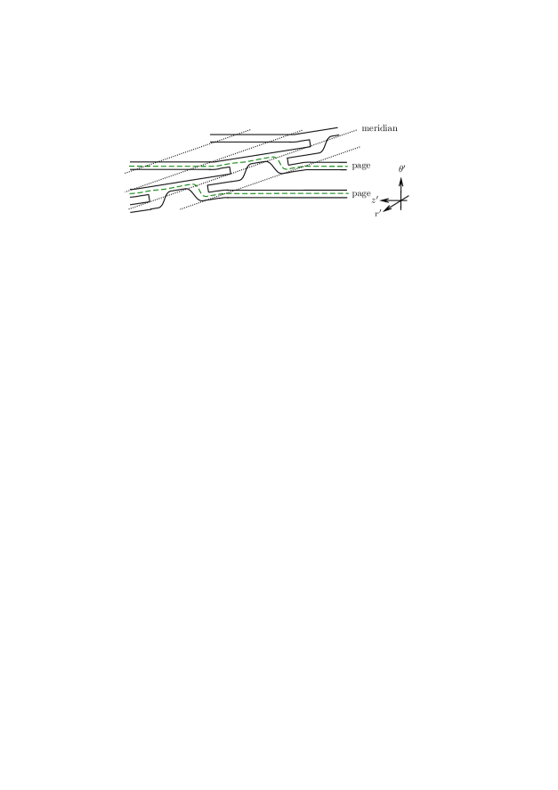
Figure 20. Mutual positions of $N_{P}$, pages and the meridians of the open book on $\partial\mathrm{Nbd}(L;M)$.

We may set the position of the pages of the open book in $M\setminus\mathrm{Int\,}\mathrm{Nbd}(L;M)$ in such a way that the pages are transverse to $R_{\alpha^{\prime}}$ since the Reeb flow of $\alpha^{\prime}$ is carried by $\hat{P}_{6}$. However, it is not always possible to choose positions of pages of the open book in $\mathrm{Nbd}(L;M)$ so that $R_{\alpha^{\prime}}$ is transverse to the pages in $\mathrm{Nbd}(L;M)$. For example, if $R_{\alpha^{\prime}}$ is winding along $L$ in the direction opposite to the open book then definitely we cannot choose such positions. For this reason, we need to reconstruct $\alpha^{\prime}$ in $\mathrm{Nbd}(L;M)$ such that $R_{\alpha^{\prime}}$ is transverse to the pages of an open book in $\mathrm{Nbd}(L;M)$.

Let $D^{2}_{s}\times S^{1}$ be the solid torus equipped with the contact form $\alpha_{b}=h_{1}(r)dz+h_{2}(r)d\theta$, where $D^{2}_{s}$ is the $2$-disk with radius $s>0$, $(r,\theta)$ are the polar coordinates of $D^{2}_{s}$, and $h_{1}(r)$ and $h_{2}(r)$ are functions such that

• $(h_{1}(0),h_{2}(0))=(1,0)$,

• $\left(\frac{dh_{1}}{dr}(0),\frac{dh_{2}}{dr}(0)\right)=(0,1)$,

• $h_{1}$ is monotone decreasing and $h_{2}$ is monotone increasing.

The curve $(h_{1}(r),h_{2}(r))$ is given as shown in Figure 21. Note that $\alpha_{b}$ is a contact form and its Reeb vector field $R_{\alpha_{b}}$ is parallel to $-\frac{dh_{1}}{dr}(r)\frac{\partial}{\partial\theta}+\frac{dh_{2}}{dr}(r)\frac{\partial}{\partial z}$ in the same direction.

Figure 21. The curve $(h_{1}(r),h_{2}(r))$.

Let $g_{T}$ be a diffeomorphism from $N_{T}^{\prime}=\{(r,\theta,z)\in D^{2}_{s}\times S^{1}\mid s^{\prime}\leq r\leq s\}$ to $N_{T}$ that maps $\partial D_{s^{\prime}}\times\{p\}$, $p\in S^{1}$, to the meridians of the open book and $\{q\}\times S^{1}$, $q\in\partial D_{s^{\prime}}$, to the pages in $N_{T}$, where $s^{\prime}$ is a positive real number with $s^{\prime}<s$ that is sufficiently close to $s$, and further satisfies that

• $g_{T}^{*}\eta=\nu_{1}(\theta,z)d\theta+\nu_{2}(\theta,z)dz$ with $\nu_{1}(\theta,z)>0$ and $\nu_{2}(\theta,z)\geq 0$, and

• $R_{\alpha_{b}}$ is positively transverse to $\ker(g_{T}^{*}\eta)$.

We may choose such a diffeomorphism as shown in Figure 22.

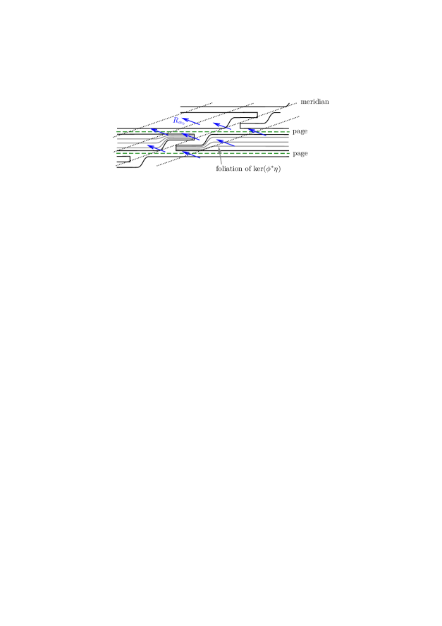
Figure 22. Mutual positions of the preimages of $N_{P}$, pages and the meridians of the open book by $g_{T}$, the Reeb vector field $R_{\alpha_{b}}$ (blue arrows) and the foliations of $\ker(g_{T}^{*}\eta)$ (drawn in gray) on $\partial\mathrm{Nbd}(L;M)$.

Set $\alpha_{c}=g_{T}^{*}(\alpha^{\prime})$. We define a contact form $\alpha_{T}$ on $N_{T}$ as

$$\alpha_{T}=(1-\chi(r))\alpha_{b}+\chi(r)\alpha_{c},$$

where $\chi$ is a monotone increasing smooth function which is $0$ for $r\leq s^{\prime}$ and $1$ for $r\geq s$. Then

$$\begin{split}\alpha_{T}\land d\alpha_{T}=&(1-\chi(r))^{2}\alpha_{b}\land d\alpha_{b}+\frac{d\chi}{dr}(r)\alpha_{b}\land dr\land\alpha_{c}\\ &+(1-\chi(r))\chi(r)(\alpha_{b}\land d\alpha_{c}+\alpha_{c}\land d\alpha_{b})+\chi(r)^{2}\alpha_{c}\land d\alpha_{c}.\end{split}$$

The second term is $\frac{d\chi}{dr}(r)\alpha_{b}\land dr\land\alpha_{c}=\frac{d\chi}{dr}(r)(h_{1}(r)dz+h_{2}(r)d\theta)\land dr\land g_{T}^{*}(\hat{\beta}_{M}+R\eta)$. Since $g_{T}^{*}\eta=\nu_{1}(\theta,z)d\theta+\nu_{2}(\theta,z)dz$ with $\nu_{1}(\theta,z)>0$ and $\nu_{2}(\theta,z)\geq 0$ by the condition (i), we have

$$(h_{1}(r)dz+h_{2}(r)d\theta)\land dr\land g_{T}^{*}\eta=(h_{1}(r)\nu_{1}(\theta,z)-h_{2}(r)\nu_{2}(\theta,z))dz\land dr\land d\theta.$$

We choose $s>0$ to be sufficiently small, which implies that $h_{2}(r)$ is sufficiently small and hence $(h_{1}(r)\nu_{1}(\theta,z)-h_{2}(r)\nu_{2}(\theta,z))dz\land dr\land d\theta>0$. Choosing $R$ to be sufficiently large, we may conclude that the second term is non-negative.

Now we observe the third term. Substituting $\alpha_{c}=g_{T}^{*}(\hat{\beta}_{M}+R\eta)$, we have

$$\alpha_{b}\land d\alpha_{c}+\alpha_{c}\land d\alpha_{b}=\alpha_{b}\land g_{T}^{*}(d\hat{\beta}_{M})+g_{T}^{*}(\hat{\beta}_{M}+R\eta)\land d\alpha_{b},$$

where we used $d\eta=0$ on $N_{D}\setminus(\hat{W}\cup\check{W})$ in Property (b) in Section 2.5. Note that $N_{T}\cap(\hat{W}\cup\check{W})=\emptyset$ due to the choice of the coordinates $(u,v,w)$ in the first paragraph of this proof. Since $R_{\alpha_{b}}$ is positively transverse to $\ker\eta$ due to the condition (ii), we have $g_{T}^{*}\eta\land d\alpha_{b}>0$. Hence the third term is positive for a sufficiently large $R$. Thus $\alpha_{T}$ is a contact form on $N_{T}$. This means that we can glue the contact forms $\alpha^{\prime}$ on $M\setminus\mathrm{Int\,}\mathrm{Nbd}(L;M)$ and $\alpha_{b}$ on $\mathrm{Nbd}(L;M)$ along $N_{T}=g_{T}(N_{T}^{\prime})$ via the gluing map $g_{T}$. We denote the obtained contact form on $M$ by $\alpha^{\prime\prime}$.

We can extend $\hat{P}_{6}$ in $M\setminus\mathrm{Int\,}\mathrm{Nbd}(L;M)$ into $\mathrm{Nbd}(L;M)$ such that the vector field $R_{\alpha^{\prime\prime}}$ is positively transverse to $\hat{P}_{6}$ in $\mathrm{Nbd}(L;M)$. Thus the Reeb flow of $\alpha^{\prime\prime}$ is carried by $\hat{P}_{6}$. We can also extend the pages of the open book in $M\setminus\mathrm{Int\,}\mathrm{Nbd}(L;M)$ into $\mathrm{Nbd}(L;M)$ with the binding $L=\{0\}\times S^{1}\subset D_{s}\times S^{1}$ such that $R_{\alpha^{\prime\prime}}$ is transverse to the interior of the pages and tangent to $L$. Thus $R_{\alpha^{\prime\prime}}$ is a monodromy vector field of the open book. This completes the proof. ∎

Proof of Theorem 1.1.

Let $\xi$ be the given contact structure on $M$. By Theorem 2.1, there exist an open book decomposition of $M$ and a contact form $\alpha$ on $M$ such that the Reeb vector field $R_{\alpha}$ is a monodromy vector field of the open book. We may assume that the genus of the page of this open book is at least $2$ and the binding is connected by using plumbings of positive Hopf bands. Note that this modification of the open book does not change the contact structure [17]. Let $P$ and $\alpha^{\prime\prime}$ be the positive flow-spine of $M$ and the contact form on $M$ obtained in the proof of Proposition 3.2, where the Reeb flow of $\alpha^{\prime\prime}$ is carried by $P$ and gives a monodromy vector field of the open book. Since $\ker\alpha$ and $\ker\alpha^{\prime\prime}$ are supported by the same open book, there exists a one-parameter family of contact forms from $\ker\alpha$ to $\ker\alpha^{\prime\prime}$ [6] and hence, by Gray’s stability [7], there exists a contactomorphism $\psi$ from $(M,\ker\alpha)$ to $(M,\ker\alpha^{\prime\prime})$. Thus, we have proved that, for the given contact structure $\ker\alpha$, $\psi^{*}\alpha^{\prime\prime}$ is a contact form such that $\ker\alpha=\ker\psi^{*}\alpha^{\prime\prime}$ and the flow generated by the Reeb vector field $R_{\psi^{*}\alpha^{\prime\prime}}$ is carried by the positive flow-spine $\psi^{-1}(\hat{P}_{6})$. That is, $\ker\alpha$ is supported by $\psi^{-1}(\hat{P}_{6})$. This completes the proof. ∎

The next is a corollary of Theorem 1.1.

Corollary 3.3.

Any flow-spine can be deformed to a positive flow-spine by applying first and second regular moves successively.

Proof.

For any homotopy class of non-singular flows, there exists a contact structure whose Reeb flow belongs to the same homotopy class [2]. By Theorem 1.1, any contact structure is supported by a positive flow-spine. Therefore, we can find a sequence of regular moves that relates a given flow-spine with the positive one by Theorem 2.2. ∎

References

- [1] Benedetti, R., Petronio, C., Branched standard spines of -manifolds, Lecture Notes in Mathematics 1653, Springer-Verlag, Berlin, 1997.
- [2] Eliashberg, Y. Classification of overtwisted contact structures on 3-manifolds, Invent. Math. 98 (1989), no. 3, 623–637.
- [3] Endoh, M., Ishii, I., A new complexity for 3-manifolds, Japan. J. Math. (N.S.) 31 (2005), 131–156.
- [4] Etnyre, J. B., Lectures on open book decompositions and contact structures, Floer homology, gauge theory, and low-dimensional topology, 103–141, Clay Math. Proc., 5, Amer. Math. Soc., Providence, RI, 2006.
- [5] Geiges, H., An introduction to contact topology, Cambridge Studies in Advanced Mathematics 109, Cambridge University Press, Cambridge, 2008.
- [6] Giroux, E., Géométrie de contact: de la dimension trois vers les dimensions supérieures, Proceedings of the International Congress of Mathematicians, Vol. II (Beijing, 2002), 405–414, Higher Ed. Press, Beijing, 2002.
- [7] Gray, J. W., Some global properties of contact structures, Ann. of Math. (2) 69 (1959), 421–450.
- [8] Ishii, I., Flows and spines, Tokyo J. Math. 9 (1986), 505–525.
- [9] Ishii, I., Moves for flow-spines and topological invariants of -manifolds, Tokyo J. Math. 15 (1992), 297–312.
- [10] Ishii, I., Ishikawa, M., Koda, Y., Naoe, H., Positive flow-spines and contact -manifolds, to appear in Annali di Matematica Pura ed Applicata (1923 -), arXiv:1912.05774 [math.GT]
- [11] Koda, Y., Branched spines and Heegaard genus of 3-manifolds, Manuscripta Mathematica 123 (2007), no. 3, 285–299.
- [12] Martinet, J., Formes de contact sur les variétiés de dimension 3, Lecture Notes in Mathematics 209, pp. 142–163, 1971.
- [13] Matveev, S., Algorithmic Topology and Classification of 3-manifolds, Algorithms and Computation in Mathematics, 9. Springer-Verlag, Berlin, 2003.
- [14] Ozbagci, B., Stipsicz, A.I., Surgery on Contact 3-manifolds and Stein Surfaces, Bolyai Society Mathematical Studies 13, Springer, 2004.
- [15] Petronio, C., Generic flows on -manifolds, Kyoto J. Math. 55 (2015), no. 1, 143–167.
- [16] Thurston, W., Winkelnkemper, H., On the existence of contact forms, Proc. Amer. Math. Soc. 52 (1975), 345–347.
- [17] Torisu, I., Convex contact structures and fibered links in 3-manifolds, Int. Math. Res. Not. 9 (2000), 441–454.