The role of dephasing for dark state coupling in a molecular Tavis-Cummings model

Abstract

Collective coupling of an ensemble of particles to a light field is commonly described by the Tavis–Cummings model. This model includes numerous eigenstates which are optically decoupled from the optically bright polariton states. To access these dark states requires breaking the symmetry in the corresponding Hamiltonian. In this paper, we investigate the influence of non-unitary processes on the dark state dynamics in molecular Tavis–Cummings model. The system is modelled with a Lindblad equation that includes pure dephasing, as they would be caused by weak interactions with an environment, and photon decay. Our simulations show that the rate of the pure dephasing, as well as the number of particles, has a significant influence on the dark state population.

I Introduction

Polaritonic chemistry—where chemical reactions are studied in the prescience of a strongly coupled electromagnetic field—is continuing to attract interest in fields ranging from chemistry to quantum optics, as shown by recent review studies [1, 2, 3, 4, 5, 6, 7]. These systems have been explored in what is becoming a rich landscape of different experiments. Examples includes demonstrating single-molecule strong coupling [8], investigating vibrational strong coupling [9, 10, 11], strong coupling in J-aggregates [12], photo-isomerization [13, 14], and two-dimensional spectroscopy of polaritonic systems [15, 16]. Along with experiments, the community has also made significant theoretical advancements. Among the investigated phenomena, we can highlight studies of conical intersections [17, 18, 19], photon up-conversion [20], polaritonic spectra [21, 22], photo-dissociation [23, 24], and model refinements from the Cavity-Born-Oppenheimer approximation [25, 26].

One of many challenges for this developing field is to build models that incorporate the details relevant for chemical reactivity (e.g. molecular vibrations along reaction coordinates) together with collective ensemble effects (several molecules coupled to the cavity field) [27, 28]. Thus, in the last decade, several studies have turned their attention to such models of emitter ensembles [29, 27, 30, 24].

In these ensemble models, a common feature is the presence of dark states, which do not couple to the field of the cavity or an external field. These states are most straightforward to consider in a Tavis-Cummings model limited to a single excitation [31]: With $N$ identical emitters, there are two bright polaritonic states, $|UP\rangle$, and $|LP\rangle$, which are symmetrical under emitter permutation. The remaining $N-1$ polaritonic states are dark. See Fig. 1. In the Tavis-Cummings model, dark states are: degenerate [32], asymmetrical under emitter permutation [33, 34], have no transition dipole moment, and correspond to collective emitter excitations, which gain no population during Hamiltonian evolution [24]. Note that these dark states emerge in the ensemble system, which is different from disallowed transitions in individual emitters.

The absence of population in the dark states makes intuitive sense; assuming an initial symmetrical state, the Hamiltonian treats all emitters identically, so unitary evolution cannot induce asymmetry. The existence of the dark states, as well as their properties, are also quite robust; for example, they persist even if the field couplings vary among emitters [35]. In this work, the model will be an extended version of Tavis-Cummings model, but properties of the dark states still hold (degeneracy, asymmetry, non-existent transition dipole moment, and zero population under Hamiltonian evolution).

Figure 1: Schematic representation of the Tavis-Cummings model. The upper $|UP\rangle$ and lower polartion state $|LP\rangle$ are split by a collective Rabi frequency. The $N-1$ dark states $|DS\rangle$ do not couple to the electromagnetic field and are thus unaffected by the cavity. Line broadening, cause by dephasing for example, introduces a coupling of the dark states with the polariton states.

Since the dark states are often assumed not to take part in the dynamics, they are commonly discarded them from the deployed models. However, there are numerous publications discussing how these states are physically significant. They have been studied in the broader context of cavity QED, [32, 36, 37, 38, 39, 40], quantum thermodynamics [41], and polaritonic chemistry [42, 27, 43, 44]. In the latter context, these states are important both when the electromagnetic field couples to electronically excited states [45, 46, 47, 48, 17], and vibrational states [49, 33, 50, 51, 52]. Despite the theoretical focus of numerous studies, the presence of dark states is by no means disregarded experimental studies [15, 53, 54, 55, 56, 57, 58, 59].

The role of dephasing processes and its influence on dark-state dynamics is intertwined with identifying a mechanism for their population [48]. To lift the decoupling of the dark states from the bright polariton states, an asymmetry in the Hamiltonian (or the Liouvilian) is required. To find such a process, we can consider processes that operate at the level of individual emitters, such as the interactions with each emitter’s environment. We model this with dephasing operators, which can be included in the equations of motion by means of the Lindblad equation:

$$\partial_{t}\hat{\rho}=-\frac{\mathchoice{}{\hskip 1.0pt}{}{}\text{i}}{\hbar}\big{[}\hat{H}\!,\hat{\rho}\big{]}+\sum_{n}\Big{(}\hat{L}_{n}\hat{\rho}\hat{L}^{\dagger}_{n}-\frac{1}{2}\big{[}\hat{L}_{n}^{\dagger}\hat{L}_{n},\hat{\rho}\big{]}_{+}\Big{)}\,.$$ (1)

The emitter dephasing can be motivated by fluctuations in the relative energies between the states in the emitter systems [60], or by a build-up of system–environment correlations [61].

In the context of strongly coupled molecular systems, there has been a recent focus on the utility of modelling decay processes with the Lindblad equation [62, 23, 63]. A consequence of using a density matrix based time evolution, however, is an increase in computational complexity. For the situation where only decay processes out of the Hilbert space under consideration are involved, an effective non-Hermitian Hamiltonian together with a Schrödinger equation can be used [64, 65, 66]. However, when dephasing becomes relevant, such simplifications will be harder to make.

The quantum trajectories method (also called the stochastic Schrödinger equation [67] or Monte Carlo wave function [68] method) can be used to bypass the explicit evaluation of the density matrix. Here, we use this method to time-evolve the Lindblad equation using an ensemble of stochastic pure-state evolutions [69, 68]. Quantum trajectories are not yet widely used for polaritonic chemistry problems, but some studies have started to emerge [70].

In this work, we investigate the role of dephasing for molecular strong coupling and its effects on the dark state dynamics. We include the effects of both dephasing and photon decay. The model is based on the Lindblad equation and implemented with quantum trajectories.

II System and model

The model system is based on an optical cavity with a single carbon monoxide molecule, where the fundamental cavity mode is resonant with a transition between the ${}^{1}\Sigma^{+}$ ground-state and an ${}^{1}\Pi$ electronically excited state in the CO molecule. To simulate a many particle system with dark states, which is also resonant with the cavity mode, $N$ two-level systems are added to the Hamiltonian. The Hamiltonian is thus an extension of the Tavis-Cummings model [4] (an optical cavity with $N$ two-level systems under the rotating wave approximation), where the extension is the the CO molecule with its internuclear coordinate.

The Hamiltonian consists of the following five parts,

$$\hat{H}=\hat{H}_{c}+\hat{H}_{a}+\hat{H}_{ca}+\hat{H}_{m}+\hat{H}_{cm}\,,$$ (2)

where $\hat{H}_{c}$ corresponds to a single fundamental mode of linearly polarized light in an optical cavity, $\hat{H}_{a}$ are the $N$ two-level emitter systems (or atoms), $\hat{H}_{ca}$ are all the resonant cavity–atom interactions, $\hat{H}_{m}$ is the CO molecule, $\hat{H}_{cm}$ is the cavity–molecule interaction.

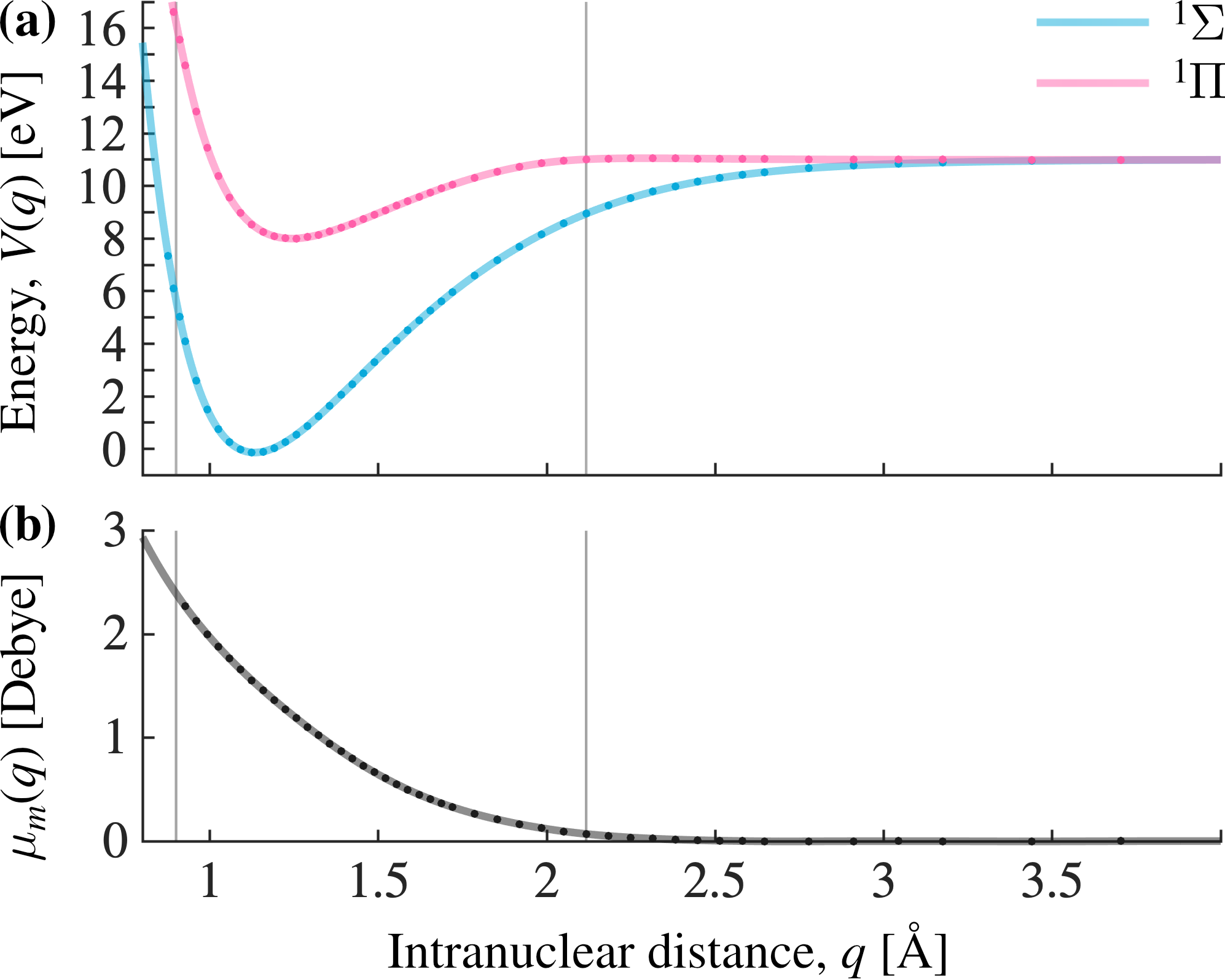
Figure 2: Potential energy curves and transition dipole curves for the CO molecule. Dots marks frozen internuclear distances from the quantum chemistry calculation. Vertical lines surround the region used in the time-evolution. (a) Potential energy surfaces for the ${}^{1}\Sigma$ ground-state and one ${}^{1}\Pi$ excited state. (b) Transition dipole moment between ${}^{1}\Sigma$ and ${}^{1}\Pi$.

The cavity mode is modelled in the Fock-basis $\{|0\rangle,|1\rangle,|2\rangle,\cdots\}$, and described by the following Hamiltonian:

$$\hat{H}_{c}=\hbar\omega_{c}\,\hat{a}^{\dagger}\!\hat{a}\,,$$ (3)

where $\hat{a}^{\dagger}$ and $\hat{a}$ are the photon creation and annihilation operators respectively, and $\omega_{c}$ is the cavity mode frequency. The cavity photon energy is fixed at $\hbar\omega_{c}=8.27\;$eV ($\lambda=150\;$nm), which makes the transition between electronic states in the CO molecule resonant with the cavity. This choice puts the minima of the two potentials at similar energies, and prevents population from accumulating in either well, see Fig. 3.

In addition to the CO molecule, the optical cavity contains $N$ two-level emitters (or atoms), where $N\in\{$0, 1, 2, 3, 5, 8, 13, 22, 36, 60$\}$ is a modulated parameter.

$$\hat{H}_{a}=\sum_{n=1}^{N}\hbar\omega_{a}\,\hat{\sigma}_{n}^{\dagger}\!\hat{\sigma}_{n}\,,$$ (4)

where $|g_{n}\rangle$ and $|e_{n}\rangle$ are the ground and excited state of the $n$-th two-level system, respectively. The operators $\hat{\sigma}_{n}=|g_{n}\rangle\!\langle e_{n}|$ and $\hat{\sigma}_{n}^{\dagger}=|e_{n}\rangle\!\langle g_{n}|$ de-excite and excite the $n$-th two-level system, respectively. The energy of the transition is chosen to be resonant to the cavity’s photon energy, $\hbar\omega_{a}=\hbar\omega_{c}=8.27\;$eV.

The interaction between emitters and cavity mode is derived under the dipole and the rotating wave approximations:

$$\hat{H}_{ca}=\sum_{n=1}^{N}\mathcal{E}_{c}(N)\,\mu_{a}\big{(}\hat{a}^{\dagger}\hat{\sigma}_{n}+\hat{a}\,\hat{\sigma}_{n}^{\dagger}\big{)}\,.$$ (5)

The transition dipole moments of all two-level systems, $\mu_{a}$, are identical, and set to $1.5$ Debye, which is on the same order of magnitude as the CO molecule (see Fig. 2(b)).

The CO molecule is modelled by including its electronic ${}^{1}\Sigma$ ground-state potential energy curve, and one of the two electronically excited ${}^{1}\Pi$ states, which has a non-zero transition dipole $\mu(q)$ moment perpendicular to the molecular axis, and is assumed to be aligned with the field polarisation. The molecular Hamiltonian reads:

$$\hat{H}_{m}=-\frac{\hbar^{2}}{2M}\frac{\text{d}^{2}}{\text{d}q^{2}}+\hat{V}_{\varSigma}(q)|\varSigma\rangle\!\langle\varSigma|+\hat{V}_{\varPi}(q)|\varPi\rangle\!\langle\varPi|\,.$$ (6)

Here, the first term is the kinetic energy of the nuclei, with the reduced mass of the CO molecule ($M=12\;498\;m_{e}$). The potential energy curves for $V_{\varSigma}(q)$ and $V_{\varPi}(q)$ are shown in Fig. 2(a).

The previous choice of photon energy makes the molecular transition resonant with the cavity mode at an internuclear distance of $q=1.17$ Å.

$$\hat{H}_{cm}=\mathcal{E}_{c}(N)\,\mu_{m}(q)\Big{(}\hat{a}^{\dagger}|\varSigma\rangle\!\langle\varPi|+\hat{a}|\varPi\rangle\!\langle\varSigma|\Big{)}\\$$ (7)

The transition dipole moment $\mu_{m}(\hat{q})$ varies between about 0 and 3 Debye according to Fig. 2(b). The vacuum electric field strength, $\mathcal{E}_{c}(N)$ is the same as the atoms are experiencing (see Eq. (5)).

The vacuum electric field strength, $\mathcal{E}_{c}(N)$, in Eqs. (5) and (7), is fixed at $3.00\;\text{V}\!/\text{nm}$ for a single CO molecule model with no atoms (i.e. $N=0$). To compensate for an increase in collective coupling strength, as we increase the number of atoms in the model, the vacuum field strength is scaled by $1/\sqrt{N+1}$ [48].

$$\mathcal{E}_{c}(N)=\frac{3.00}{\sqrt{N+1}}\,\hskip 2.0pt\text{V}\!/\text{nm}$$ (8)

Note that the effects of single particle coupling strength can not be directly compared to a collective coupling strength of equal size. Thus, the results are expected to show a different behavior [24].

The highest single particle cavity coupling strength, $g_{\text{avg}}=\mathcal{E}_{c}\mu_{\text{avg}}$, occurs for $N=0$. We compare this to the typical energy scale, $g_{\text{avg}}/\hbar\omega_{c}=0.011$. The system operates well below the ultra-strong coupling regime. Note that we assumed an average transition dipole moment of $\mu_{\text{avg}}=1.5$ Debye.

In addition to the unitary part of the Hamiltonian, there are two non-unitary physical processes, which are introduced through the Lindblad equation (1). The Lindblad framework assumes that, that the system-bath correlations times are short enough to allow for the Markovian approximation [71, 49]. Thus, our results address interactions that can be modelled as non-Markovian.

The first non-unitary process is single-emitter dephasing of the CO molecule and all $N$ two-level systems. The corresponding rate of dephasing, $\gamma$, is the key parameter whose effects we aim to investigate. It is the same for all emitters, which have their individual dephasing operator

$$\hat{L}_{n}\mathrel{\vbox{\hbox{.}\hbox{.}}}\hskip 0.8pt=\sqrt{\!\frac{\gamma}{2}}\;\hat{\sigma}_{z}^{(n)}\,,$$ (9)

where, $\hat{\sigma}_{z}^{(n)}$ is the third Pauli matrix for the $n$-th emitter:

$$\hat{\sigma}_{z}=\begin{bmatrix}1&0\\ 0&-1\end{bmatrix}\,.$$ (10)

Other choices of this operator yield the same time-evolution. However, this choice is beneficial for the quantum trajectory method, since it does not transfer population between states [72].

When constructing the Lindblad dephasing operators, we neglect the fact that the sub-systems are coupled (by the cavity mode) and build them phenomenologically. This is generally considered acceptable outside the ultra-strong coupling regime [73, 74]. In the appendix, section VIII.1, we discuss the potential problems with this approach, and argue that the phenomenological operators are appropriate.

The second non-unitary process is photon decay caused by a lossy cavity. The Lindblad operator for a single cavity mode, with the photon decay rate $\kappa$, reads:

$$\hat{L}_{c}\mathrel{\vbox{\hbox{.}\hbox{.}}}\hskip 0.8pt=\sqrt{\kappa}\,\hat{a}\,.$$ (11)

The photon lifetime is fixed at $\tau=100\;$fs, yielding $\kappa=1/\tau=0.01\;\text{fs}^{-1}$. For the chosen photon energy at $\hbar\omega_{c}=8.27\;$eV, this corresponds to a quality factor of $Q=1.26\times 10^{3}$. For comparison, Q-factors reported in the literature range from $10^{1}$ [54, 75] for plasmonic nanoparticles [8] to $10^{4}$ [76, 77, 75] for Fabry–Pérot cavities made of Bragg reflectors.

III Methods

Our studied observable is energy retention, i.e. we consider the fraction of the initial excitation that, despite the photon decay, remains in the system after 500 fs. The duration is chosen in relation to the timescale of the nuclear dynamics and mirrors previous investigations [24, 62]. The initial excitation consists of the cavity mode being is in its first excited (single photon) state, while all emitters are in their ground-states. This limits the total number of excitations to one, which allows us to truncate the basis.

A direct solution of the Lindblad equation (1) with a density matrix scales quadratically with the number of states involved. Such an approach becomes prohibitive as the number of atoms in our system increases. Instead of modelling a statistical state as a single density operator, we use quantum trajectories [69, 68] to obtain the statistics from an ensemble of pure state wave functions. Thus, the cost is shifted from a single memory consuming density matrix, to running multiple, but lighter, pure-state calculations with wave functions, $\{\psi_{i}(t)\}$. Each wave function evolves stochastically, with "quantum jumps" occurring randomly in proportion to physical parameters. One can prove that in the limit of an infinite ensemble of wave functions, the state from evolution with quantum trajectories approaches the state from the Lindblad equation [68].

From the ensemble of $N_{T}$ trajectories, $\{\psi_{i}(t):i\in 1\cdots N_{T}\}$, a density matrix can be recovered by summing outer products of each wave function with a uniform weight:

$$\hat{\rho}=\frac{1}{N_{T}}\sum_{i=1}^{N_{T}}|\psi_{i}\rangle\!\langle\psi_{i}|\,.$$ (12)

Expectation values $\{\langle\hat{A}_{i}\rangle\}$ can also be obtained directly from the weighted sum of all trajectories, without having to construct $\hat{\rho}$ explicitly:

$$\text{Tr}\big{[}\hat{A}\hat{\rho}\big{]}=\frac{1}{N_{T}}\sum_{i=1}^{N_{T}}\langle\hat{A}_{i}\rangle\,.$$ (13)

The quantum trajectory method requires two modifications to the time-dependent Schrödinger equation. The first one adds the last term from Eq. (1), i.e. $\sum_{n}-1/2\,[\hat{L}_{n}^{\dagger}\hat{L}_{n},\hat{\rho}]_{+}$, to the Hamiltonian in the form of a norm-decaying term. However, in our choice of implementation, the wave function is continuously renormalized (at each discrete time-step). Using the Lindblad operators from Eqs. (9) and (11) leads to the non-Hermitian Hamiltonian:

$$\hat{H}^{\prime}\mathrel{\vbox{\hbox{.}\hbox{.}}}\hskip 0.8pt=\hat{H}-\mathchoice{}{\hskip 1.0pt}{}{}\text{i}\hbar\frac{\kappa}{2}\,\hat{a}^{\dagger}\!\hat{a}-\mathchoice{}{\hskip 1.0pt}{}{}\text{i}\hbar\frac{\gamma}{2}\sum_{n}\big{(}\hat{\sigma}_{z}^{(n)}\big{)}^{\!\dagger}\hat{\sigma}_{z}^{(n)}\,.$$ (14)

The second term in Eq. (14), is responsible for the photon decay, while the third term only affects the norm of the total wave function, since $\big{(}\hat{\sigma}_{z}^{(n)}\big{)}^{\dagger}\hat{\sigma}_{z}^{(n)}=\hat{\mathbbm{1}}$. The algorithm used for the propagation renormalizes the wave function in each step, thus the last term from Eq. (14) has no effect and can be removed.

The second part that is required for in the quantum trajectories method are discrete, stochastic jumps. These jumps originate from the first term in Eq. (1), i.e. $\sum_{n}\hat{L}_{n}\hat{\rho}\hat{L}^{\dagger}_{n}$. The probability of a jump occurring during a time-interval $\Delta\hskip 1.0ptt$ depends on the rates $\kappa$ and $\gamma$ as well as the population in the subspace from which the jump occurs:

$$P\big{(}\hskip 1.0pt\text{jump with }\hat{L}_{k}\text{ during }\Delta t\big{)}=\Delta\hskip 1.0ptt\langle\varPsi(t)|\hat{L}^{\dagger}_{k}\hat{L}_{k}|\varPsi(t)\rangle\,.$$ (15)

Note here that the Lindblad operators $L_{k}$ include the rates, $\kappa$ and $\gamma$, as shown in Eqs. (8) and (11). At each time-step, random numbers are generated to determine if a jump occurs, in which case the Lindblad operator $\hat{L}_{k}$, is applied to the wave function and the wave function is normalized.

We have implemented the quantum trajectories approach with our in-house software package QDng, which allows for the time evolution of wave functions. Implementations into existing methods are recurring in the literature [72, 78, 70]. For each statistical state (see Eq. (12)), $N_{T}=2500$ wave function trajectories were run. Estimates of the resulting errors are given in the caption of Fig. 4. Each wave function was time-evolved with the Arnoldi propagation method [79], at order 10 and a time-step of to $0.5\hskip 1.0pt\text{au}$ ($0.012\;\text{fs}$).

The time-evolution is carried out in a product basis composed of the field-free molecular states, the field free two-level system states, and the Fock states of the cavity mode. In the following, we will refer to this basis as product basis.

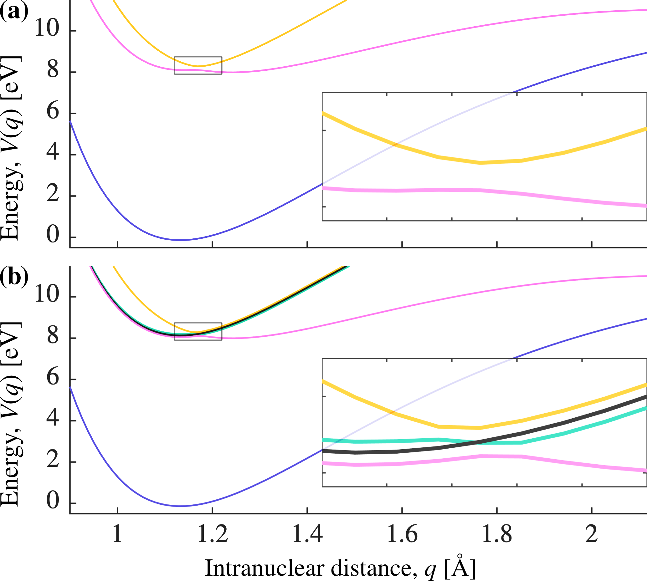
Figure 3: Potential energy surfaces of the polaritonic basis. A single CO molecule and $N=2$ two-level systems in an optical cavity. With $N=2$ the first dark state is introduced. The upper polaritonic state is yellow, the middle polaritonic state is green, the lower polaritonic state is pink, the ground-state is blue, and dark states are black. For higher values of $N>2$ the curves are essentially the same [24], but additional degenerate dark states are introduced.

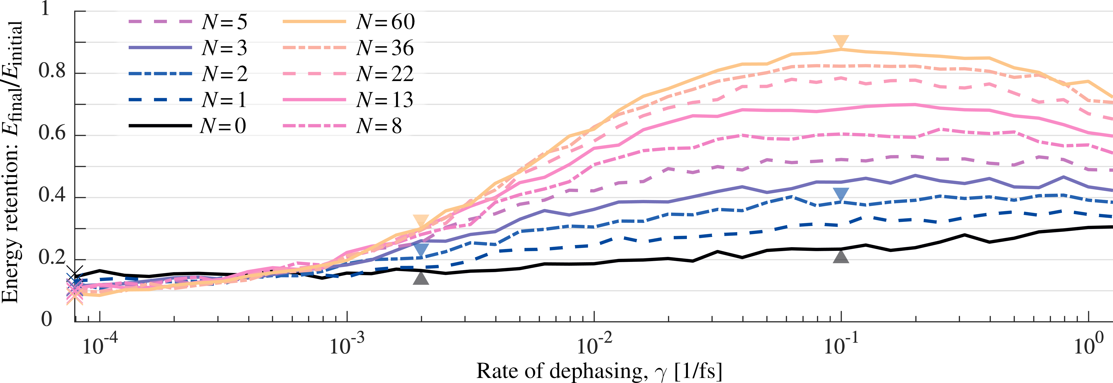
Figure 4: Energy retention in relation to dephasing rate. The vertical axis shows energy retention, i.e. the remaining energy as a fraction of initial energy, $E_{\text{final}}/E_{\text{initial}}$ where $E_{\text{initial}}=\hbar\omega_{c}$, after 500 fs of time-evolution. The horizontal axis is the single emitter dephasing rate, $\gamma$, which is the same for all emitters. Each curve corresponds to a particular number of two-level systems, $N$. The number of dark states for each curve is $N-1$. Crosses on the vertical axis shows the energy retention for $\gamma=0$. Arrows mark points where dynamics plots are supplied, see Figs. 5, 6, and 7. Standard deviations due to the Trajectories method (from a set of 25 runs) are also calculated at these points. Grey arrows both have $\sigma\approx 0.008$, left blue has $\sigma\approx 0.011$, right blue has $\sigma\approx 0.012$, left yellow has $\sigma\approx 0.009$, right yellow has $\sigma\approx 0.008$.

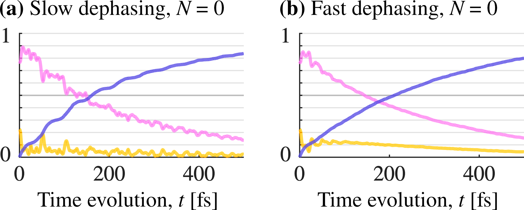
Figure 5: Population time-evolution of the polaritonic potential energy surfaces shown in Fig. 3(a). Colors match the ones used for the surfaces in Fig. 3. In the left column (a) the dephasing is slow ($\gamma\approx 0.002\;\text{fs}^{-1}$), in the right column (b) dephasing is fast ($\gamma\approx 0.09\;\text{fs}^{-1}$). The left grey arrows in Fig. 4 shows the data point of (a), and the right grey arrow is the data point for (b). The two cases, (a) and (b), behave very similar, the most apparent difference is the dampening of interference for fast dephasing, which makes the curves in (b) smoother.

For the purpose of interpreting the data (section IV) we diagonalize the potential curves, to obtain polaritonic curves (see Fig. 3). This can be achieved by a pointwise diagonalization of the Hamiltonian along the reaction coordinate, $q$, while omitting the kinetic energy operator. The number of polaritonic energy surfaces depends on $N$, but for $N>2$ all additional energy surfaces are the degenerate dark states. Thus, plotting the result for $N=0$ and $N=2$ gives an overview for all other values of $N$ (see Fig. 3(b)). Note that dark states are a feature of the polaritonic basis, and does not appear in the product basis. We ensure that uncoupled polaritonic surfaces are allowed to cross, by following the eigenvector tracking method described in [24].

The potential energy curves and dipole functions of the CO molecule, shown in Fig. 2, are the relevant results of a quantum chemistry calculation that originally included eight non-degenerate states and their respective transition dipole moments. The electronic structure calculations were carried out with the program package Molpro [80, 81, 82] at the CASSCF(10/14)/MRCI/aug-cc-pVQZ level of theory, with a state average over a total of twelve electronic states. Energies, dipole moments, and transition dipole moments are calculated at 50 internuclear distances, between 0.926 Å and 6.35 Å. The two electronic states included in this work are ${}^{1}\Sigma^{+}$ and one of the two doubly degenerate ${}^{1}\Pi$ states. The data is in good agreement with previous calculations [83, 84]. The molecular potentials and transitions moments are interpolated to a spatial grid with 96 grid points in the interval $0.90\leq q\leq 2.12$ Å (see vertical lines in Fig. 2). The result is used to construct the molecular Hamiltonians, $\hat{H}_{m}$ and $\hat{H}_{cm}$ in Eqs. (6) and (7), for the numerical calculations.

IV Results and Discussion

To construct a molecular Tavis-Cummings model, which includes dark states, $N$ two-level systems were introduced along with the CO molecule. We included the values $N\in\{$0, 1, 2, 3, 5, 8, 13, 22, 36, 60$\}$ and for each value the dephasing rate is varied between 0 and 10% of the cavity frequency $\omega_{c}$, which corresponds to the dephasing rates:  $0\leq\gamma\leq 1.26\;\text{fs}^{-1}$. After 500 fs of time evolution, the energy retention is recorded. The remaining energy in the system is then plotted as a fraction of the initial energy, in relation to the dephasing rate for each $N$. This constitutes the main result in this study and is shown in Fig. 4. Note that the obtained curves are not perfectly smooth, which is an expected result of the stochastic sampling of the density matrix.

Only 10% to 15% of the initial energy is retained in the system for the dephasing free case ($\gamma=0$, see crosses on the vertical axis in Fig. 4). With no dephasing, the $N-1$ dark states are not populated and does not impact the behavior of the system. However, even though the number of bright states are fixed, and with a constant collective coupling strength (see Eq. (8)), the energy retention for $\gamma=0$ varies. This can explained as follows: the collective Rabi splitting appears to behave similar to the single particle Rabi splitting between the upper and lower polariton. However, the splitting between middle polariton state and the upper and lower polariton state follows the single particle Rabi splitting and not the collective Rabi splitting [24].

With no two-level systems, i.e. $N=0$, the impact of dephasing on the energy retention is small (black curve in Fig. 4). Fig. 5(a) and (b), compare the populations in the polaritonic basis (from Fig. 3(a)) for a slow and fast dephasing rate (and $N=0$). The most obvious difference in the populations is the amount of oscillations caused by interference and by the avoided crossing in polaritonic states. We can understand the dampened oscillations as dephasing canceling the otherwise coherent population transfer between different trajectories.

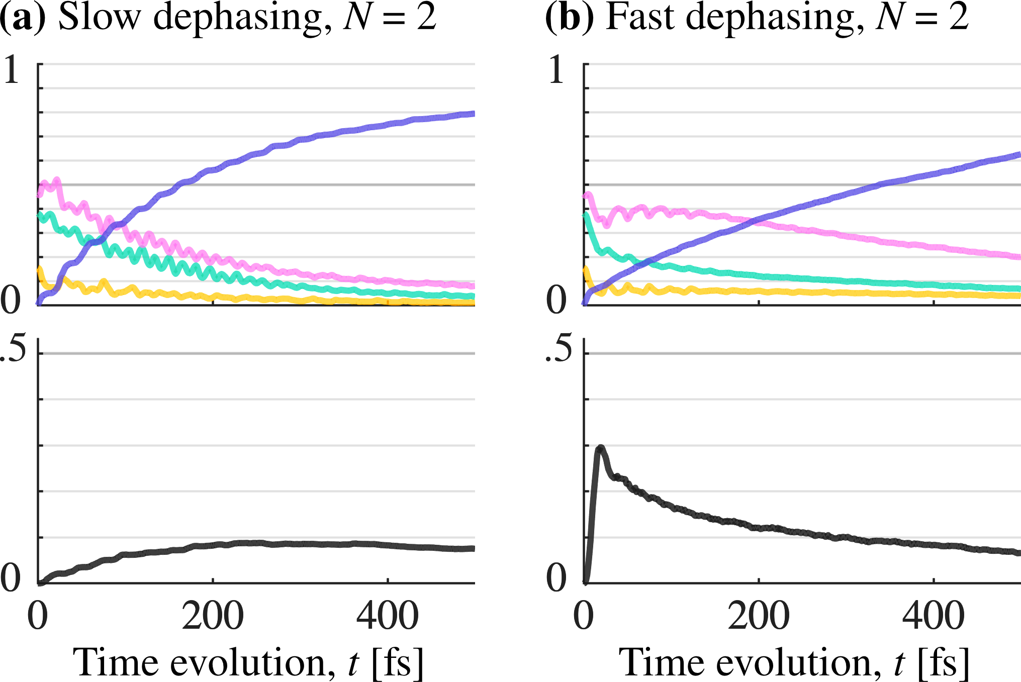
Figure 6: Population time-evolution of the polaritonic potential energy surfaces shown in Fig. 3(b). Colors match the ones used for the surfaces in Fig. 3. In the left column (a) the dephasing is slow ($\gamma\approx 0.002\,\text{fs}^{-1}$), in the right column (b) dephasing is fast ($\gamma\approx 0.09\,\text{fs}^{-1}$). The left blue arrows in Fig. 4 shows the data point of (a), and the blue arrow is the data point for (b).

Introducing dark states ($N\geq 2$) will make the energy retention increasingly sensitive to changes in the dephasing rate. We consider first the case with a single dark state ($N=2$). Here, dephasing has an observable effect on energy retention. Fig. 3(b) shows the polaritonic energy surfaces for $N=2$, which includes a single dark state (black curve) and middle polariton state (green curve). The corresponding population evolution is shown in Fig. 6, for slow dephasing (a) and fast dephasing (b). Note, how a fast dephasing rate imposes a rapid build-up of population in the dark state, which peaks at about 20 fs and slowly decays thereafter. This in contrast to the slow dephasing rate, where the dark state population occurs slowly over a timescale of $\approx 300$ fs.

The highest energy retention is observed for the largest number of two-level system studied ($N=60$) and a dephasing rate on the order of $\gamma\approx 10^{-1}\,\text{fs}^{-1}$. Here, the solid yellow curve in Fig. 4 shows a sharp increase in energy retention with increasing dephasing, from around 10 % to almost 90 %. The time-evolution of the populations for $N=60$ is shown in Fig. 7, for both slow dephasing in (a) and fast dephasing in (b). The populations of all 59 dark states are shown as a sum (black curve). For the fast dephasing rate, the dark states population builds up rapidly, and reaches its maximum value of 90 % in about 40 fs. Thereafter, the dark states population is very slowly released back to the bright states, with a retention of 80 % at 500 fs. For $N=60$ and a slow dephasing rate, the build up to about 27 % is slow, and does not reach a maximum within 500 fs. For both slow and fast dephasing, the population in the dark states has significantly increased when compared to the case $N=2$ (compare Figs. 6 and 7).

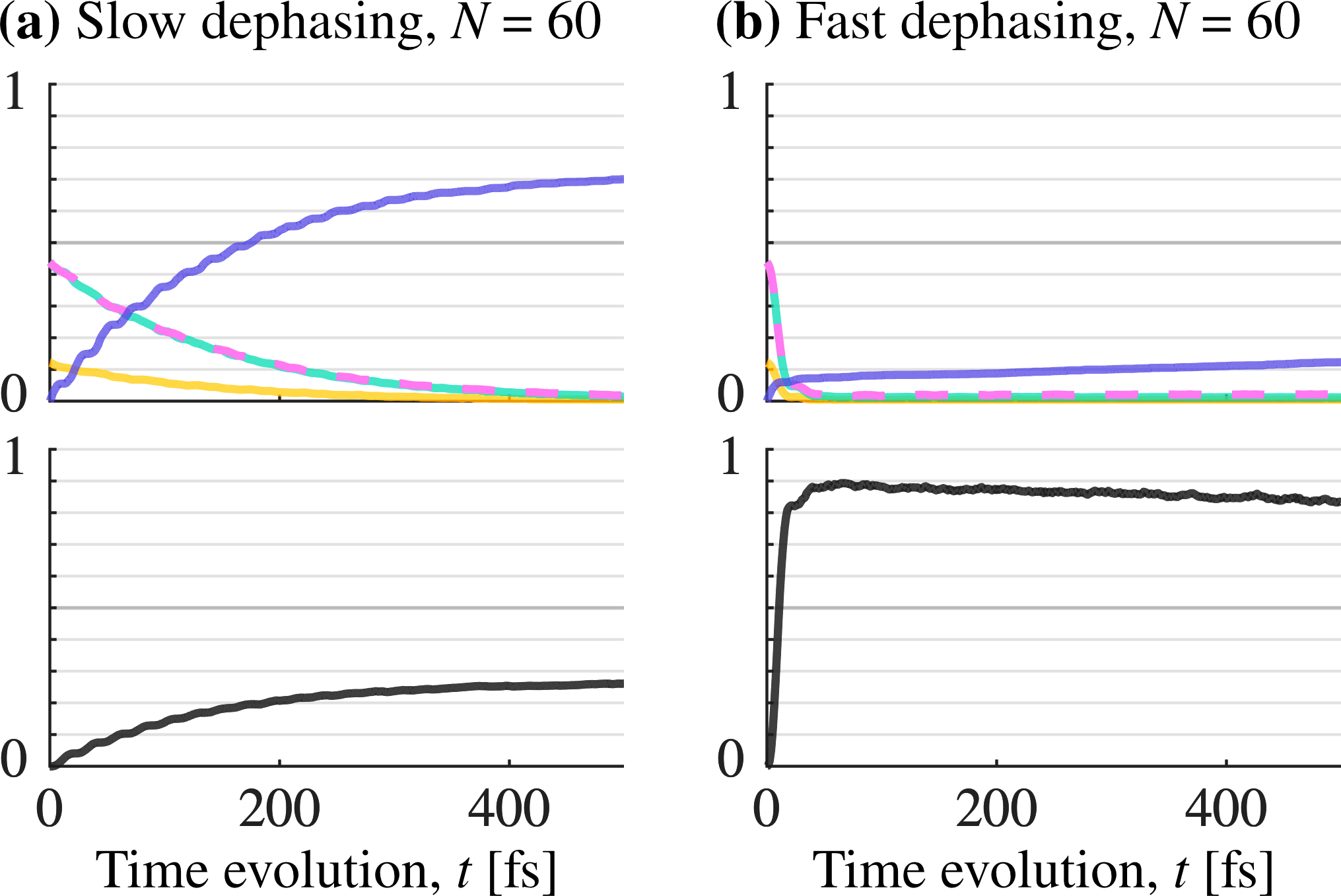
Figure 7: Population time-evolution of the polaritonic potential energy surfaces for $N=60$ (which are very similar to the ones shown in Fig. 3. Colors match the ones used for the surfaces in Fig. 3(b), but the black curve is a sum of all 59 dark states. In the left column (a) the dephasing is slow ($\gamma\approx 0.002\;\text{fs}^{-1}$), in the right column (b) dephasing is fast ($\gamma\approx 0.09\;\text{fs}^{-1}$). The left yellow arrows in Fig. 4 shows the data point of (a), and the right yellow arrow is the data point for (b).

The mechanism for the energy retention can be explained by the transition dipole moments of the collective system. The main energy loss mechanism is the decay of photons due to imperfect cavity mirrors. However, the dark states have no transition dipole moment in the absence of dephasing, as they represent asymmetric superpositions of matter excitations. Thus, the dark states do not couple to the cavity mode in an ideal system and can not scatter photons into the cavity mode. Population in the dark states are thus protected from photon decay. However, the dephasing breaks the symmetry in the Hamiltonian that decouples the dark states from the upper, middle, and lower, polariton states and enables population transfer. With an increasing number of particles $N$, the number of available dark states increases, and thus the effective rate increases with which these states are populated increases. The dark state subspace can thus serve as a reservoir which protects the systems from photon decay [49, 85].

The population transfer between dark states and bright states goes both ways. As can be seen in Figs. 6(b) and 7(b), dephasing will also slowly return the population to the bright states. However, this process is slower and than the population transfer into the dark states, resulting in an overall slow down of the energy loss.

The energy retention in Fig. 4 has a local maximum with respect to the dephasing rate at about $\gamma\approx 10^{-1}$ fs^-1 and $N=60$. In this regime, the Rabi oscillations ($\Omega_{R}=2.85\times 10^{-1}\,\text{fs}^{-1}$) are dampened, but not yet over dampened. The line width of the dark states and the polariton states are sufficiently narrow to be spectrally well separated.

However, if the dephasing rate the is further increased, the polariton states begin to overlap with the dark states. In this over dampened regime, the dark states are no longer sufficiently decoupled from the bright states, and there is a significant leakage from the dark states. This effect causes a decreased energy retention for large dephasing rates. Note that the maximum of the energy retention shifts to larger dephasing rates with decreasing $N$. Note that the decrease in energy retention, after the maximum, depends on the choice of our initial state (excited cavity), through the momentary rates populating and depopulating the dark state reservoir.

V Conclusion

In summary, we have investigated a molecular Tavis–Cummings model under the influence of dephasing and photon decay. The model system consisted of a CO molecule with a varying number of resonantly coupled two-level systems, which has been solved with a quantum trajectory approach instead of a direct solution of the Lindblad equation. This approach allowed us to use a wave function base calculation which scales more favorably with respect to the number of states than evaluating a density matrix explicitly.

In this atomistic model, we could show that the dark states become increasingly coupled to the polariton states as the dephasing rate is increased. As a result, population gets trapped in the dark states, and it is protected from photon decay processes. Our findings are in line with earlier studies [49, 85]. Under the influence of dephasing the dark states are no longer decoupled from the polariton states. The effective transfer rate into the dark states even increases with an increasing number of dark states, and thus providing an increasingly efficient protection against photon decay. In the investigated systems, the photonic excitation was rapidly transferred into the dark state reservoir and slowly released back into the bright polariton states.

Our results show that dephasing, as it would occur under experimental conditions in condensed phase, plays a significant role in the dynamics of such a system. Realistic models should thus not only include photon decay, which has been demonstrated to play a crucial role [24], but should also include the effects from pure dephasing in condensed phase.

VI Acknowledgments

This project has received funding from the European Research Council (ERC) under the European Union’s Horizon 2020 research and innovation program (grant agreement No. 852286) and European Union’s Horizon 2020 research and innovation program under the Marie Sklodowska-Curie grant agreement no. E.D. thanks Prof. Jonas Larson for valuable discussions and insightful feedback.

VII Data availability

The data that support the findings of this study are available upon reasonable request.

VIII Appendix

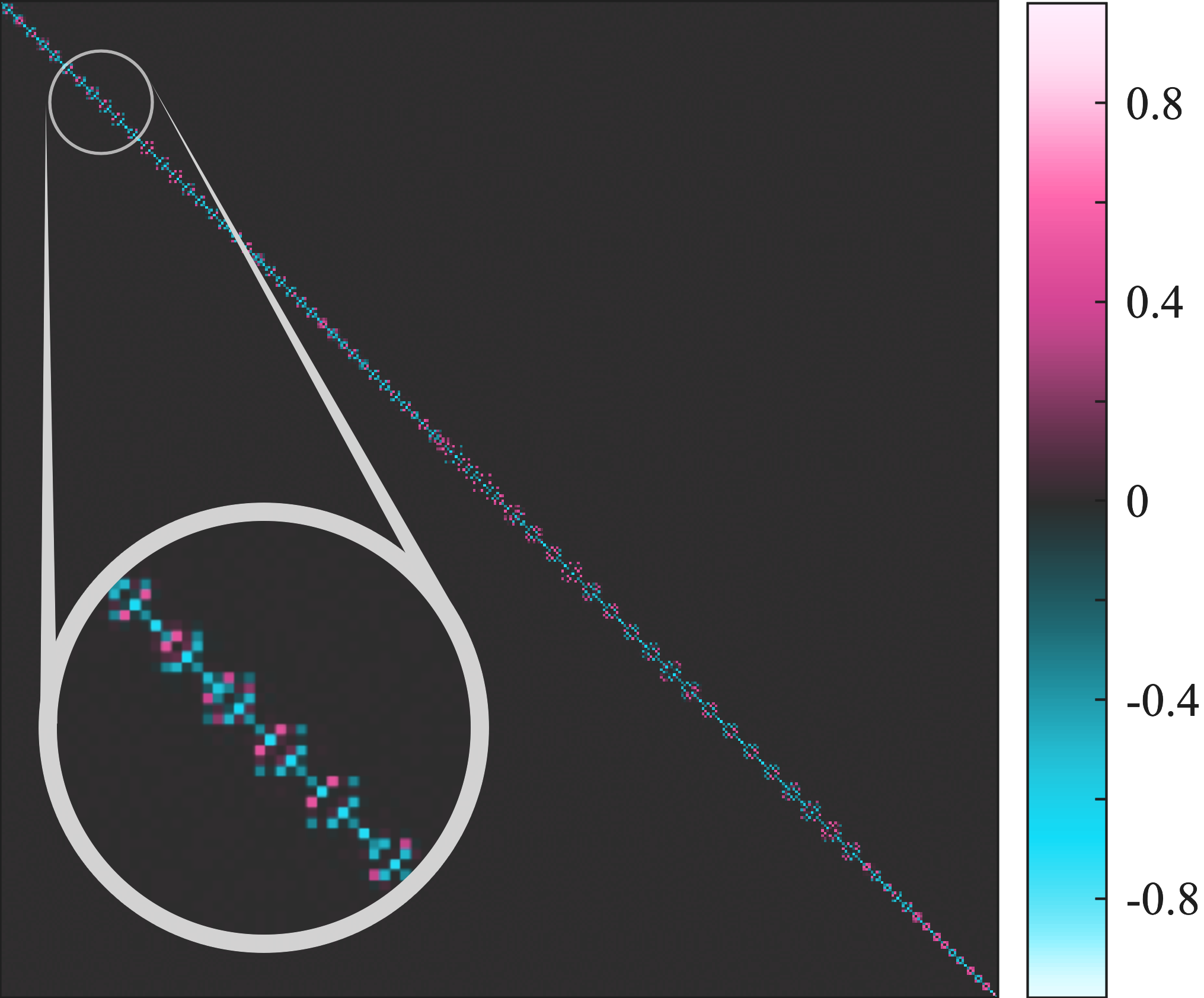
Figure 8: Dephasing operator after transformation to eigen-basis. The initially diagonal operator acquires off-diagonal elements, but the operator remains essentially block-diagonal.

VIII.1 Impacts from phenomenological dephasing operators

For a single two-level system, the dephasing operator in Eq. (9) has the expected effect; to decay away phase information without moving population between states. However, when a system is built from many strongly coupled sub-systems (such as in our case), this operator will include some unintended amount of driving and decay. To probe how significant this effect is, we can fully diagonalise the Hamiltonian from Eq. (2), and apply the basis transformation to a dephasing operator. (Note that we can omit the ground-state from the diagonalisation since it does not couple to any other state.) This basis transformation into a fully diagonalised Hamiltonian will give a set of eigenstates containing some unphysical states; when the energy of the vibrational motion is enough to dissociate the molecule. However, since our time-evolution does not exhibit dissociation we do not populate such questionable states, and they could be excluded from this analysis without affecting the conclusion.

A dephasing operator (for $N=2$ atoms) after transformation to the energy ordered eigenbasis is shown in Fig. 8. Driving and decay will appear as off-diagonal elements.

On close inspection we can see that there are off-diagonal elements, but that the matrix is essentially block diagonal. This means that there are some driving and decay between eigenstates that are close to degeneracy, but the population is trapped within each block of states. Thus, we cannot drive or decay population further than between a few energetically adjacent states. This is not of concern to our investigation and a phenomenological operator is considered sufficient. For further discussions, see for instance [86, 87, 49].

References

- Törmä and Barnes [2014] P. Törmä and W. L. Barnes, Strong coupling between surface plasmon polaritons and emitters: a review, Reports on Progress in Physics 78, 013901 (2014), https://doi.org/10.1088/0034-4885/78/1/013901 .
- Flick et al. [2017a] J. Flick, M. Ruggenthaler, H. Appel, and A. Rubio, Atoms and molecules in cavities, from weak to strong coupling in quantum-electrodynamics (qed) chemistry, Proceedings of the National Academy of Sciences 114, 3026 (2017a), https://www.pnas.org/doi/pdf/10.1073/pnas.1615509114 .
- Ribeiro et al. [2018] R. F. Ribeiro, L. A. Mart\́mathchoice{}{\hskip1.0pt}{}{}\text{i}nez-Mart\́mathchoice{}{\hskip1.0pt}{}{}\text{i}nez, M. Du, J. Campos-Gonzalez-Angulo, and J. Yuen-Zhou, Polariton chemistry: controlling molecular dynamics with optical cavities, Chem. Sci. 9, 6325 (2018), http://dx.doi.org/10.1039/C8SC01043A .
- Frisk Kockum et al. [2019] A. Frisk Kockum, A. Miranowicz, S. De Liberato, S. Savasta, and F. Nori, Ultrastrong coupling between light and matter, Nature Reviews Physics 1, 19 (2019), https://doi.org/10.1038/s42254-018-0006-2 .
- Hertzog et al. [2019] M. Hertzog, M. Wang, J. Mony, and K. Börjesson, Strong light–matter interactions: a new direction within chemistry, Chem. Soc. Rev. 48, 937 (2019), http://dx.doi.org/10.1039/C8CS00193F .
- Hirai et al. [2020] K. Hirai, J. A. Hutchison, and H. Uji-i, Recent progress in vibropolaritonic chemistry, ChemPlusChem 85, 1981 (2020), https://chemistry-europe.onlinelibrary.wiley.com/doi/pdf/10.1002/cplu.202000411 .
- Fregoni et al. [2022] J. Fregoni, F. J. Garcia-Vidal, and J. Feist, Theoretical challenges in polaritonic chemistry, ACS Photonics 9, 1096 (2022), https://doi.org/10.1021/acsphotonics.1c01749 .
- Chikkaraddy et al. [2016] R. Chikkaraddy, B. de Nijs, F. Benz, S. J. Barrow, O. A. Scherman, E. Rosta, A. Demetriadou, P. Fox, O. Hess, and J. J. Baumberg, Single-molecule strong coupling at room temperature in plasmonic nanocavities, Nature 535, 127 (2016).
- Simpkins et al. [2015] B. S. Simpkins, K. P. Fears, W. J. Dressick, B. T. Spann, A. D. Dunkelberger, and J. C. Owrutsky, Spanning strong to weak normal mode coupling between vibrational and fabry–pérot cavity modes through tuning of vibrational absorption strength, ACS Photonics 2, 1460 (2015), https://doi.org/10.1021/acsphotonics.5b00324 .
- Damari et al. [2019] R. Damari, O. Weinberg, D. Krotkov, N. Demina, K. Akulov, A. Golombek, T. Schwartz, and S. Fleischer, Strong coupling of collective intermolecular vibrations in organic materials at terahertz frequencies, Nature Communications 10, 3248 (2019).
- Thomas et al. [2019] A. Thomas, L. Lethuillier-Karl, K. Nagarajan, R. M. A. Vergauwe, J. George, T. Chervy, A. Shalabney, E. Devaux, C. Genet, J. Moran, and T. W. Ebbesen, Tilting a ground-state reactivity landscape by vibrational strong coupling, Science 363, 615 (2019), https://www.science.org/doi/pdf/10.1126/science.aau7742 .
- Munkhbat et al. [2018] B. Munkhbat, M. Wersäll, D. G. Baranov, T. J. Antosiewicz, and T. Shegai, Suppression of photo-oxidation of organic chromophores by strong coupling to plasmonic nanoantennas, Science Advances 4, eaas9552 (2018), https://www.science.org/doi/pdf/10.1126/sciadv.aas9552 .
- Hutchison et al. [2012] J. A. Hutchison, T. Schwartz, C. Genet, E. Devaux, and T. W. Ebbesen, Modifying chemical landscapes by coupling to vacuum fields, Angewandte Chemie International Edition 51, 1592 (2012), https://onlinelibrary.wiley.com/doi/pdf/10.1002/anie.201107033 .
- Mony et al. [2021] J. Mony, C. Climent, A. U. Petersen, K. Moth-Poulsen, J. Feist, and K. Börjesson, Photoisomerization efficiency of a solar thermal fuel in the strong coupling regime, Advanced Functional Materials 31, 2010737 (2021), https://onlinelibrary.wiley.com/doi/pdf/10.1002/adfm.202010737 .
- Xiang et al. [2018] B. Xiang, R. F. Ribeiro, A. D. Dunkelberger, J. Wang, Y. Li, B. S. Simpkins, J. C. Owrutsky, J. Yuen-Zhou, and W. Xiong, Two-dimensional infrared spectroscopy of vibrational polaritons, Proceedings of the National Academy of Sciences 115, 4845 (2018), https://www.pnas.org/doi/pdf/10.1073/pnas.1722063115 .
- Mewes et al. [2020] L. Mewes, M. Wang, R. A. Ingle, K. Börjesson, and M. Chergui, Energy relaxation pathways between light-matter states revealed by coherent two-dimensional spectroscopy, Communications Physics 3, 157 (2020).
- Ulusoy et al. [2019] I. S. Ulusoy, J. A. Gomez, and O. Vendrell, Modifying the nonradiative decay dynamics through conical intersections via collective coupling to a cavity mode, The Journal of Physical Chemistry A 123, 8832 (2019), pMID: 31536346, https://doi.org/10.1021/acs.jpca.9b07404 .
- Fábri et al. [2021] C. Fábri, G. J. Halász, L. S. Cederbaum, and Á. Vibók, Born–oppenheimer approximation in optical cavities: from success to breakdown, Chem. Sci. 12, 1251 (2021).
- Couto and Kowalewski [2022] R. C. Couto and M. Kowalewski, Suppressing non-radiative decay of photochromic organic molecular systems in the strong coupling regime, Phys. Chem. Chem. Phys. 24, 19199 (2022).
- Gudem and Kowalewski [2022] M. Gudem and M. Kowalewski, Triplet-triplet annihilation dynamics of naphthalene, Chemistry – A European Journal 28, e202200781 (2022), https://chemistry-europe.onlinelibrary.wiley.com/doi/pdf/10.1002/chem.202200781 .
- Flick and Narang [2018] J. Flick and P. Narang, Cavity-correlated electron-nuclear dynamics from first principles, Phys. Rev. Lett. 121, 113002 (2018).
- Fischer and Saalfrank [2021] E. W. Fischer and P. Saalfrank, Ground state properties and infrared spectra of anharmonic vibrational polaritons of small molecules in cavities, The Journal of Chemical Physics 154, 104311 (2021), https://doi.org/10.1063/5.0040853 .
- Torres-Sánchez and Feist [2021] J. Torres-Sánchez and J. Feist, Molecular photodissociation enabled by ultrafast plasmon decay, The Journal of Chemical Physics 154, 014303 (2021), https://doi.org/10.1063/5.0037856 .
- Davidsson and Kowalewski [2020a] E. Davidsson and M. Kowalewski, Atom assisted photochemistry in optical cavities, The Journal of Physical Chemistry A 124, 4672 (2020a), pMID: 32392061, https://doi.org/10.1021/acs.jpca.0c03867 .
- Flick et al. [2017b] J. Flick, H. Appel, M. Ruggenthaler, and A. Rubio, Cavity born–oppenheimer approximation for correlated electron–nuclear-photon systems, Journal of Chemical Theory and Computation 13, 1616 (2017b), pMID: 28277664, https://doi.org/10.1021/acs.jctc.6b01126 .
- Schnappinger and Kowalewski [2023] T. Schnappinger and M. Kowalewski, Nonadiabatic wave packet dynamics with ab initio cavity-born-oppenheimer potential energy surfaces, Journal of Chemical Theory and Computation 19, 460 (2023), pMID: 36625723, https://doi.org/10.1021/acs.jctc.2c01154 .
- Sidler et al. [2021] D. Sidler, C. Schäfer, M. Ruggenthaler, and A. Rubio, Polaritonic chemistry: Collective strong coupling implies strong local modification of chemical properties, The Journal of Physical Chemistry Letters 12, 508 (2021), pMID: 33373238, https://doi.org/10.1021/acs.jpclett.0c03436 .
- Schäfer [2022] C. Schäfer, Polaritonic chemistry from first principles via embedding radiation reaction, The Journal of Physical Chemistry Letters 13, 6905 (2022), pMID: 35866694, https://doi.org/10.1021/acs.jpclett.2c01169 .
- Herrera and Spano [2016] F. Herrera and F. C. Spano, Cavity-controlled chemistry in molecular ensembles, Phys. Rev. Lett. 116, 238301 (2016), https://link.aps.org/doi/10.1103/PhysRevLett.116.238301 .
- Sommer et al. [2021] C. Sommer, M. Reitz, F. Mineo, and C. Genes, Molecular polaritonics in dense mesoscopic disordered ensembles, Phys. Rev. Research 3, 033141 (2021), https://link.aps.org/doi/10.1103/PhysRevResearch.3.033141 .
- Tavis and Cummings [1968] M. Tavis and F. W. Cummings, Exact solution for an -molecule—radiation-field hamiltonian, Phys. Rev. 170, 379 (1968), https://link.aps.org/doi/10.1103/PhysRev.170.379 .
- Houdré et al. [1996] R. Houdré, R. P. Stanley, and M. Ilegems, Vacuum-field rabi splitting in the presence of inhomogeneous broadening: Resolution of a homogeneous linewidth in an inhomogeneously broadened system, Phys. Rev. A 53, 2711 (1996), https://link.aps.org/doi/10.1103/PhysRevA.53.2711 .
- Herrera and Spano [2017] F. Herrera and F. C. Spano, Theory of nanoscale organic cavities: The essential role of vibration-photon dressed states, ACS Photonics 5, 65 (2017), https://doi.org/10.1021/acsphotonics.7b00728 .
- Hernández and Herrera [2019] F. J. Hernández and F. Herrera, Multi-level quantum rabi model for anharmonic vibrational polaritons, The Journal of Chemical Physics 151, 144116 (2019), https://doi.org/10.1063/1.5121426 .
- López et al. [2007] C. E. López, H. Christ, J. C. Retamal, and E. Solano, Effective quantum dynamics of interacting systems with inhomogeneous coupling, Phys. Rev. A 75, 033818 (2007), https://link.aps.org/doi/10.1103/PhysRevA.75.033818 .
- Yang et al. [1999] G. J. Yang, O. Zobay, and P. Meystre, Two-atom dark states in electromagnetic cavities, Phys. Rev. A 59, 4012 (1999), https://link.aps.org/doi/10.1103/PhysRevA.59.4012 .
- Zheng [2007] S.-B. Zheng, Nongeometric phase gates via adiabatic passage of dark states in cavity qed, Physics Letters A 362, 125 (2007), https://www.sciencedirect.com/science/article/pii/S0375960106015428 .
- White et al. [2019] D. H. White, S. Kato, N. Német, S. Parkins, and T. Aoki, Cavity dark mode of distant coupled atom-cavity systems, Phys. Rev. Lett. 122, 253603 (2019), https://link.aps.org/doi/10.1103/PhysRevLett.122.253603 .
- Botzung et al. [2020] T. Botzung, D. Hagenmüller, S. Schütz, J. Dubail, G. Pupillo, and J. Schachenmayer, Dark state semilocalization of quantum emitters in a cavity, Phys. Rev. B 102, 144202 (2020), https://link.aps.org/doi/10.1103/PhysRevB.102.144202 .
- Zanner et al. [2022] M. Zanner, T. Orell, C. M. F. Schneider, R. Albert, S. Oleschko, M. L. Juan, M. Silveri, and G. Kirchmair, Coherent control of a multi-qubit dark state in waveguide quantum electrodynamics, Nature Physics 18, 538 (2022), https://doi.org/10.1038/s41567-022-01527-w .
- Scholes et al. [2020] G. D. Scholes, C. A. DelPo, and B. Kudisch, Entropy reorders polariton states, The Journal of Physical Chemistry Letters 11, 6389 (2020), pMID: 32678609, https://doi.org/10.1021/acs.jpclett.0c02000 .
- Gonzalez-Ballestero et al. [2016] C. Gonzalez-Ballestero, J. Feist, E. Gonzalo Bad\́mathchoice{}{\hskip1.0pt}{}{}\text{i}a, E. Moreno, and F. J. Garcia-Vidal, Uncoupled dark states can inherit polaritonic properties, Phys. Rev. Lett. 117, 156402 (2016), https://link.aps.org/doi/10.1103/PhysRevLett.117.156402 .
- Gera and Sebastian [2022] T. Gera and K. L. Sebastian, Effects of disorder on polaritonic and dark states in a cavity using the disordered tavis–cummings model, The Journal of Chemical Physics 156, 194304 (2022), https://doi.org/10.1063/5.0086027 .
- Cederbaum [2022] L. S. Cederbaum, Cooperative molecular structure in polaritonic and dark states, The Journal of Chemical Physics 156, 184102 (2022), https://doi.org/10.1063/5.0090047 .
- Vendrell [2018] O. Vendrell, Collective jahn-teller interactions through light-matter coupling in a cavity, Phys. Rev. Lett. 121, 253001 (2018), https://link.aps.org/doi/10.1103/PhysRevLett.121.253001 .
- Groenhof et al. [2019] G. Groenhof, C. Climent, J. Feist, D. Morozov, and J. J. Toppari, Tracking polariton relaxation with multiscale molecular dynamics simulations, The Journal of Physical Chemistry Letters 10, 5476 (2019), pMID: 31453696, https://doi.org/10.1021/acs.jpclett.9b02192 .
- Climent et al. [2022] C. Climent, D. Casanova, J. Feist, and F. J. Garcia-Vidal, Not dark yet for strong light-matter coupling to accelerate singlet fission dynamics, Cell Reports Physical Science 3, 100841 (2022), https://www.sciencedirect.com/science/article/pii/S2666386422001151 .
- Tichauer et al. [2022] R. H. Tichauer, D. Morozov, I. Sokolovskii, J. J. Toppari, and G. Groenhof, Identifying vibrations that control non-adiabatic relaxation of polaritons in strongly coupled molecule–cavity systems, The Journal of Physical Chemistry Letters 13, 6259 (2022), pMID: 35771724, https://doi.org/10.1021/acs.jpclett.2c00826 .
- del Pino et al. [2015] J. del Pino, J. Feist, and F. J. Garcia-Vidal, Quantum theory of collective strong coupling of molecular vibrations with a microcavity mode, New Journal of Physics 17, 053040 (2015), https://doi.org/10.1088/1367-2630/17/5/053040 .
- Campos-Gonzalez-Angulo et al. [2019] J. A. Campos-Gonzalez-Angulo, R. F. Ribeiro, and J. Yuen-Zhou, Resonant catalysis of thermally activated chemical reactions with vibrational polaritons, Nature Communications 10, 4685 (2019), https://doi.org/10.1038/s41467-019-12636-1 .
- Xiang et al. [2019] B. Xiang, R. F. Ribeiro, L. Chen, J. Wang, M. Du, J. Yuen-Zhou, and W. Xiong, State-selective polariton to dark state relaxation dynamics, The Journal of Physical Chemistry A 123, 5918 (2019), pMID: 31268708, https://doi.org/10.1021/acs.jpca.9b04601 .
- Du and Yuen-Zhou [2022] M. Du and J. Yuen-Zhou, Catalysis by dark states in vibropolaritonic chemistry, Phys. Rev. Lett. 128, 096001 (2022), https://link.aps.org/doi/10.1103/PhysRevLett.128.096001 .
- Eizner et al. [2019] E. Eizner, L. A. Mart\́mathchoice{}{\hskip1.0pt}{}{}\text{i}nez-Mart\́mathchoice{}{\hskip1.0pt}{}{}\text{i}nez, J. Yuen-Zhou, and S. Kéna-Cohen, Inverting singlet and triplet excited states using strong light-matter coupling, Science Advances 5, eaax4482 (2019), https://www.science.org/doi/pdf/10.1126/sciadv.aax4482 .
- Wersäll et al. [2019] M. Wersäll, B. Munkhbat, D. G. Baranov, F. Herrera, J. Cao, T. J. Antosiewicz, and T. Shegai, Correlative dark-field and photoluminescence spectroscopy of individual plasmon–molecule hybrid nanostructures in a strong coupling regime, ACS Photonics 6, 2570 (2019), https://doi.org/10.1021/acsphotonics.9b01079 .
- Liu et al. [2020] B. Liu, V. M. Menon, and M. Y. Sfeir, The role of long-lived excitons in the dynamics of strongly coupled molecular polaritons, ACS Photonics 7, 2292 (2020), https://doi.org/10.1021/acsphotonics.0c00895 .
- DelPo et al. [2020] C. A. DelPo, B. Kudisch, K. H. Park, S.-U.-Z. Khan, F. Fassioli, D. Fausti, B. P. Rand, and G. D. Scholes, Polariton transitions in femtosecond transient absorption studies of ultrastrong light–molecule coupling, The Journal of Physical Chemistry Letters 11, 2667 (2020), pMID: 32186878, https://doi.org/10.1021/acs.jpclett.0c00247 .
- Avramenko and Rury [2021] A. G. Avramenko and A. S. Rury, Local molecular probes of ultrafast relaxation channels in strongly coupled metalloporphyrin-cavity systems, The Journal of Chemical Physics 155, 064702 (2021), https://doi.org/10.1063/5.0055296 .
- Cohn et al. [0] B. Cohn, S. Sufrin, A. Basu, and L. Chuntonov, Vibrational polaritons in disordered molecular ensembles, The Journal of Physical Chemistry Letters 0, 8369 (0), pMID: 36043884, https://doi.org/10.1021/acs.jpclett.2c02341 .
- Avramenko and Rury [2022] A. G. Avramenko and A. S. Rury, Cavity polaritons formed from spatially separated quasi-degenerate porphyrin excitons: Structural modulations of bright and dark state energies and compositions, The Journal of Physical Chemistry C 126, 15776 (2022), https://doi.org/10.1021/acs.jpcc.2c04121 .
- Marquardt and Püttmann [2008] F. Marquardt and A. Püttmann, Introduction to dissipation and decoherence in quantum systems 10.48550/ARXIV.0809.4403 (2008), https://arxiv.org/abs/0809.4403 .
- Costa et al. [2016] A. C. S. Costa, M. W. Beims, and W. T. Strunz, System-environment correlations for dephasing two-qubit states coupled to thermal baths, Phys. Rev. A 93, 052316 (2016), https://link.aps.org/doi/10.1103/PhysRevA.93.052316 .
- Davidsson and Kowalewski [2020b] E. Davidsson and M. Kowalewski, Simulating photodissociation reactions in bad cavities with the lindblad equation, The Journal of Chemical Physics 153, 234304 (2020b), https://doi.org/10.1063/5.0033773 .
- Wellnitz et al. [2021] D. Wellnitz, G. Pupillo, and J. Schachenmayer, A quantum optics approach to photoinduced electron transfer in cavities, The Journal of Chemical Physics 154, 054104 (2021), https://doi.org/10.1063/5.0037412 .
- Ulusoy and Vendrell [2020] I. S. Ulusoy and O. Vendrell, Dynamics and spectroscopy of molecular ensembles in a lossy microcavity, The Journal of Chemical Physics 153, 044108 (2020), https://doi.org/10.1063/5.0011556 .
- Antoniou et al. [2020] P. Antoniou, F. Suchanek, J. F. Varner, and J. J. Foley, Role of cavity losses on nonadiabatic couplings and dynamics in polaritonic chemistry, The Journal of Physical Chemistry Letters 11, 9063 (2020), pMID: 33045837, https://doi.org/10.1021/acs.jpclett.0c02406 .
- Felicetti et al. [2020] S. Felicetti, J. Fregoni, T. Schnappinger, S. Reiter, R. de Vivie-Riedle, and J. Feist, Photoprotecting uracil by coupling with lossy nanocavities, The Journal of Physical Chemistry Letters 11, 8810 (2020), pMID: 32914984, https://doi.org/10.1021/acs.jpclett.0c02236 .
- Coccia et al. [2020] E. Coccia, J. Fregoni, C. A. Guido, M. Marsili, S. Pipolo, and S. Corni, Hybrid theoretical models for molecular nanoplasmonics, The Journal of Chemical Physics 153, 200901 (2020), https://doi.org/10.1063/5.0027935 .
- Mølmer et al. [1993] K. Mølmer, Y. Castin, and J. Dalibard, Monte carlo wave-function method in quantum optics, J. Opt. Soc. Am. B 10, 524 (1993), http://opg.optica.org/josab/abstract.cfm?URI=josab-10-3-524 .
- Dalibard et al. [1992] J. Dalibard, Y. Castin, and K. Mølmer, Wave-function approach to dissipative processes in quantum optics, Phys. Rev. Lett. 68, 580 (1992), https://link.aps.org/doi/10.1103/PhysRevLett.68.580 .
- Triana and Herrera [2022] J. F. Triana and F. Herrera, Open quantum dynamics of strongly coupled oscillators with multi-configuration time-dependent hartree propagation and markovian quantum jumps, The Journal of Chemical Physics 157, 194104 (2022), https://doi.org/10.1063/5.0119293 .
- Manzano [2020] D. Manzano, A short introduction to the lindblad master equation, AIP Advances 10, 025106 (2020), https://doi.org/10.1063/1.5115323 .
- Coccia et al. [2018] E. Coccia, F. Troiani, and S. Corni, Probing quantum coherence in ultrafast molecular processes: An ab initio approach to open quantum systems, The Journal of Chemical Physics 148, 204112 (2018), https://doi.org/10.1063/1.5022976 .
- Beaudoin et al. [2011] F. Beaudoin, J. M. Gambetta, and A. Blais, Dissipation and ultrastrong coupling in circuit qed, Phys. Rev. A 84, 043832 (2011), https://link.aps.org/doi/10.1103/PhysRevA.84.043832 .
- Salmon et al. [2022] W. Salmon, C. Gustin, A. Settineri, O. D. Stefano, D. Zueco, S. Savasta, F. Nori, and S. Hughes, Gauge-independent emission spectra and quantum correlations in the ultrastrong coupling regime of open system cavity-qed, Nanophotonics 11, 1573 (2022), https://doi.org/10.1515/nanoph-2021-0718 .
- Franke et al. [2020] S. Franke, M. Richter, J. Ren, A. Knorr, and S. Hughes, Quantized quasinormal-mode description of nonlinear cavity-qed effects from coupled resonators with a fano-like resonance, Phys. Rev. Res. 2, 033456 (2020).
- Najer et al. [2019] D. Najer, I. Söllner, P. Sekatski, V. Dolique, M. C. Löbl, D. Riedel, R. Schott, S. Starosielec, S. R. Valentin, A. D. Wieck, N. Sangouard, A. Ludwig, and R. J. Warburton, A gated quantum dot strongly coupled to an optical microcavity, Nature 575, 622 (2019).
- Wellnitz et al. [2022] D. Wellnitz, G. Pupillo, and J. Schachenmayer, Disorder enhanced vibrational entanglement and dynamics in polaritonic chemistry, Communications Physics 5, 120 (2022).
- Mandal et al. [2022] S. Mandal, F. Gatti, O. Bindech, R. Marquardt, and J.-C. Tremblay, Multidimensional stochastic dissipative quantum dynamics using a lindblad operator, The Journal of Chemical Physics 156, 094109 (2022), https://doi.org/10.1063/5.0079735 .
- Smyth et al. [1998] E. S. Smyth, J. S. Parker, and K. T. Taylor, Numerical integration of the time-dependent schrödinger equation for laser-driven helium, Comput. Phys. Commun. 114, 1 (1998).
- Werner et al. [2012] H.-J. Werner, P. J. Knowles, G. Knizia, F. R. Manby, and M. Schütz, Molpro: a general-purpose quantum chemistry program package, WIREs Computational Molecular Science 2, 242 (2012), https://wires.onlinelibrary.wiley.com/doi/pdf/10.1002/wcms.82 .
- Werner et al. [2020] H.-J. Werner, P. J. Knowles, F. R. Manby, J. A. Black, K. Doll, A. Heßelmann, D. Kats, A. Köhn, T. Korona, D. A. Kreplin, Q. Ma, T. F. Miller, A. Mitrushchenkov, K. A. Peterson, I. Polyak, G. Rauhut, and M. Sibaev, The molpro quantum chemistry package, The Journal of Chemical Physics 152, 144107 (2020), https://doi.org/10.1063/5.0005081 .
- [82] H.-J. Werner, P. J. Knowles, P. Celani, W. Györffy, A. Hesselmann, D. Kats, G. Knizia, A. Köhn, T. Korona, D. Kreplin, R. Lindh, Q. Ma, F. R. Manby, A. Mitrushenkov, G. Rauhut, M. Schütz, K. R. Shamasundar, T. B. Adler, R. D. Amos, S. J. Bennie, A. Bernhardsson, A. Berning, J. A. Black, P. J. Bygrave, R. Cimiraglia, D. L. Cooper, D. Coughtrie, M. J. O. Deegan, A. J. Dobbyn, K. Doll, M. Dornbach, F. Eckert, S. Erfort, E. Goll, C. Hampel, G. Hetzer, J. G. Hill, M. Hodges, T. Hrenar, G. Jansen, C. Köppl, C. Kollmar, S. J. R. Lee, Y. Liu, A. W. Lloyd, R. A. Mata, A. J. May, B. Mussard, S. J. McNicholas, W. Meyer, T. F. Miller III, M. E. Mura, A. Nicklass, D. P. O’Neill, P. Palmieri, D. Peng, K. A. Peterson, K. Pflüger, R. Pitzer, I. Polyak, M. Reiher, J. O. Richardson, J. B. Robinson, B. Schröder, M. Schwilk, T. Shiozaki, M. Sibaev, H. Stoll, A. J. Stone, R. Tarroni, T. Thorsteinsson, J. Toulouse, M. Wang, M. Welborn, and B. Ziegler, Molpro, version 2020.1, a package of ab initio programs, see https://www.molpro.net.
- Shi et al. [2013] D.-H. Shi, W.-T. Li, J.-F. Sun, and Z.-L. Zhu, Theoretical study of spectroscopic and molecular properties of several low-lying electronic states of co molecule, International Journal of Quantum Chemistry 113, 934 (2013), https://onlinelibrary.wiley.com/doi/pdf/10.1002/qua.24036 .
- O’Neil and Schaefer [1970] S. V. O’Neil and H. F. Schaefer, Valence-excited states of carbon monoxide, The Journal of Chemical Physics 53, 3994 (1970), https://doi.org/10.1063/1.1673871 .
- Quach et al. [2022] J. Q. Quach, K. E. McGhee, L. Ganzer, D. M. Rouse, B. W. Lovett, E. M. Gauger, J. Keeling, G. Cerullo, D. G. Lidzey, and T. Virgili, Superabsorption in an organic microcavity: Toward a quantum battery, Science Advances 8, eabk3160 (2022), https://www.science.org/doi/pdf/10.1126/sciadv.abk3160 .
- Scala et al. [2007] M. Scala, B. Militello, A. Messina, J. Piilo, and S. Maniscalco, Microscopic derivation of the jaynes-cummings model with cavity losses, Phys. Rev. A 75, 013811 (2007), https://link.aps.org/doi/10.1103/PhysRevA.75.013811 .
- Betzholz et al. [2020] R. Betzholz, B. G. Taketani, and J. M. Torres, Breakdown signatures of the phenomenological lindblad master equation in the strong optomechanical coupling regime, Quantum Science and Technology 6, 015005 (2020), https://dx.doi.org/10.1088/2058-9565/abc39d .