Denoising Cosine Similarity: A Theory-Driven Approach for Efficient Representation Learning

Abstract

Representation learning has been increasing its impact on the research and practice of machine learning, since it enables to learn representations that can apply to various downstream tasks efficiently. However, recent works pay little attention to the fact that real-world datasets used during the stage of representation learning are commonly contaminated by noise, which can degrade the quality of learned representations. This paper tackles the problem to learn robust representations against noise in a raw dataset. To this end, inspired by recent works on denoising and the success of the cosine-similarity-based objective functions in representation learning, we propose the denoising Cosine-Similarity (dCS) loss. The dCS loss is a modified cosine-similarity loss and incorporates a denoising property, which is supported by both our theoretical and empirical findings. To make the dCS loss implementable, we also construct the estimators of the dCS loss with statistical guarantees. Finally, we empirically show the efficiency of the dCS loss over the baseline objective functions in vision and speech domains.
Keywords: Unsupervised Representation Learning, Robust Representation Learning, Self-supervised Learning

1 INTRODUCTION

Representation Learning (RL) is one of the most popular fields in machine learning research since it improves performance in downstream tasks, e.g., supervised learning and clustering. Many RL methods have been proposed in various domains, such as vision [7, 22, 25, 27, 5, 8, 42, 16], speech [43], and language [20, 19]. In RL, an encoder is trained in order to extract useful information from raw data. However, it is pointed out by [4] that raw data obtained through sensors or other devices can be noisy. In addition, it is shown by [33] that such noisy data tends to interfere with a Neural Network (NN)-based encoder learning useful representations for downstream tasks.

To tackle representation learning in the presence of noise in data, in this study, we focus on the Denoising RL (DRL) setting:

• An unlabeled training set of raw data is given, and the raw data is noisy. The goal is to build an efficient NN-based encoder for downstream tasks using only the noisy training set.

While denoising and RL have been studied separately by many previous works, the study of the combination of these problems is little investigated despite its importance. Here, to consider how to construct an efficient algorithm under the DRL setting, we review these problems separately:

1) Denoising

Denoising methods have been proposed in various domains, such as vision [41, 37, 3, 47, 52, 71, 29, 32] and speech [70, 18, 31, 55]. The purpose of these methods is to predict the clean data of noisy data. Typically, using a noisy dataset, an AutoEncoder (AE) is trained by minimizing a loss, and then the trained AE is used as the predictor. In the vision (resp. speech) domain, for example, the AE is defined by a U-Net [54] (resp. a Wave U-Net [58]). As for the loss, in the vision domain, it is commonly defined via the Mean Squared Error (MSE) [41, 37]. On the other hand, in speech, the Cosine-Similarity (CS) loss is often employed [31, 55]. We emphasize that a trained encoder obtained under denoising purpose is not necessarily efficient for downstream tasks, as shown in our numerical experiments.

2) RL

There are two popular methods: the AE-based methods [64, 26, 43] and the self-supervised learning methods that use data augmentation [7, 22, 8]. In the AE-based methods, given an unlabeled dataset, an AE is trained by minimizing a loss, and then the trained encoder is used to extract the representation. The loss function is usually defined via the MSE [64, 26, 43]. On the other hand, in the self-supervised representation learning methods, the CS is often employed to define the objective function. In recent years, self-supervised representation learning has been studied actively in many domains, such as the vision domain [7, 9, 22, 5, 27, 8, 42, 68, 23, 16] and the language domain [20, 19], because of its high performance.

As seen above, for denoising and RL, the CS plays an important role in many domains. Thus, it is worthwhile to use CS for learning representation from noisy data. A naive approach is to learn an AE-based model by minimizing the CS between the reconstruction $\hat{\bm{s}}$ from a noisy data $\bm{x}$ and the corresponding clean data $\bm{s}$, as some similar approach with the MSE-based loss has been investigated by the previous study [69]. However, this naive approach does not work in the DRL setting since the clean $\bm{s}$ is supervised data. Inspired by the recent denoising methods that require only noisy data [37, 55], we aim to propose a modified CS loss, which can enhance the efficiency of the CS in the DRL setting. Towards achieving this goal, we propose the denoising CS (dCS) loss with the theoretically guaranteed denoising property . The dCS loss is defined without any clean data. Remarkably, the minimization of the dCS loss is closely related to that of the minimization of the CS loss defined with $\bm{b}\odot\bm{s}$ and the masked reconstruction $\bm{b}\odot\hat{\bm{s}}$ from the noisy $\tilde{\bm{x}}$, where $\bm{b}$ is a Bernoulli random vector and $\odot$ denotes the Hadamard product. Thus, the dCS loss has the potential to obtain good representation for downstream tasks of many domains, where only noisy raw data is available.

Our main contributions are summarized as follows: Firstly, we propose the dCS loss (Section 3.4) based on the theoretical background (Section 3.2). Secondly, we investigate the practical implementation of the dCS loss from the statistical estimation viewpoints (Section 3.3). Thirdly, in our numerical experiments, we show that the proposed loss can enhance the efficiency of representation learning in multiple DRL settings (Section 4).

At the end of this section, we summarize the structure of the rest of this paper. In Section 2, we introduce details of the aforementioned existing methods. Then, we discuss the connection between those methods and our dCS loss. In Section 3, we present the definition of the dCS loss and its theoretical properties. In Section 4, we demonstrate the efficiency of the proposed loss in multiple DRL settings using standard real-world datasets. Finally, we conclude this study and discuss the future work in Section 5.

2 RELATED WORK

First, in Section 2.1, details of denoising methods listed in 1) Denoising of Section 1 are introduced. Then, in Section 2.2, details of self-supervised learning methods listed in 2) RL of Section 1 are introduced. For details of the AE-based RL methods listed in 2) RL of Section 1, see Appendix B.2. In Section 2.3, the relations between those methods and the dCS loss are discussed.

2.1 Denoising Methods

Vision Domain

Lehtinen et al. [41] proposed Noise2Noise (N2N). N2N uses a set of pairs of noisy images to train a U-Net [54] with the MSE-based loss. Here, the paired noisy images share the same clean image. After the training, the trained U-Net is used to predict the clean image of the noisy image. Krull et al. [37] proposed Noise2Void (N2V), which also employs a U-Net for predicting clean image, and the loss is defined via the MSE. In contrast to N2N, N2V requires only a single noisy image. Note that N2N and N2V are self-supervised denoising methods, i.e., the minimization of these losses is equivalent to that of an MSE-based loss defined via the clean data; for the detailed mathematical arguments of N2N, see Zhussip et al. [71]. For completeness, we give an overview of the mathematical equivalence of N2V in Appendix B.1.

Speech Domain

Kashyap et al. [31] proposed a denoising method in the speech domain, partially inspired by N2N. In this method, a denoiser model is trained by a pair of noisy speech data using an objective defined via the CS loss. Although the denoising performance is competitive, the theoretical guarantee is not sufficiently discussed. Sanada et al. [55] proposed a variant of N2V (SDSD) in the speech domain, which is also based on the CS loss. In addition, they provided a theoretical guarantee to SDSD.

2.2 Self-supervised Representation Learning Methods

2.2.1 An Overview of Recent Self-supervised Representation Learning Methods

Vision Domain

Recent self-supervised representation learning has utilized the data augmentation techniques: pairs of positive samples are generated by applying data augmentation to raw data [7, 9]. Several recent works [10, 53, 11] tackle the problems where data augmentation techniques cause some inefficient effects on producing pairs of similar or dissimilar data. The learning criterion is diversifying. For instance, Chen et al. [7], He et al. [25], Henaff [27] proposed contrastive learning methods based on InfoNCE [48], which is a lower-bound of mutual information; see Poole et al. [51]. On the other hand, Grill et al. [22] proposed BYOL, whose objective is to make feature vectors of similar data points close in the feature space, a.k.a. minimization of the positive loss. Then, Chen and He [8] introduced a simplified variant of BYOL named SimSiam. Although several works [5, 42, 16, 68, 23] have shed light on contrastive learning from various perspectives, the CS is a popular choice for the similarity measure [7, 22, 25, 8, 16].

Language Domain

The self-supervised representation learning also has been studied in the language domain. For instance, Giorgi et al. [20] proposed a self-supervised learning objective for sentence embedding tasks, where the objective does not require labels for the training. Gao et al. [19] proposed a method of contrastive learning termed SimCSE, which utilizes dropout as data augmentation.

2.2.2 SimSiam Revisit

We revisit SimSiam [8] to give an instance of recent self-supervised representation learning methods. Chen and He [8] have observed that a simplified framework of BYOL [22], i.e., SimSiam, still achieved competitive performance. The loss function of SimSiam consists of the cosine similarity between pairs of similar data points. Moreover, maximization of the similarity makes similar data aligned in the feature space. In order to prevent features from being collapsed, SimSiam also employs the stop-gradient operation as BYOL does.

Here, we formulate the original framework of SimSiam, following Chen and He [8]. Let $f_{\psi}$ be an encoder, $g_{\xi}$ an additional prediction MLP, and $f_{\hat{\psi}}$ an encoder with the stop-gradient technique. Note that in the initial stage of each step in training, $f_{\hat{\psi}}$ is created by freezing the parameters of the encoder $f_{\psi}$. Let $\ell_{\rm{CS}}(\bm{u},\bm{v})$ denote the CS loss between $\bm{u}\in\mathbb{R}^{D}$ and $\bm{v}\in\mathbb{R}^{D}$:

$$\ell_{\rm{CS}}(\bm{u},\bm{v})=-\frac{\langle\bm{u},\bm{v}\rangle}{\|\bm{u}\|_{2}\|\bm{v}\|_{2}}.$$ (1)

Then, the loss function of SimSiam is defined as

$$L_{\rm SimSiam}(\psi,\xi)=\frac{1}{2}\mathbb{E}_{\bm{x}^{\prime},\bm{x}^{\prime\prime}}[\ell_{\rm{CS}}(g_{\xi}({f_{\psi}}(\bm{x}^{\prime})),f_{\hat{\psi}}(\bm{x}^{\prime\prime}))+\ell_{\rm{CS}}(g_{\xi}(f_{\psi}(\bm{x}^{\prime\prime})),f_{\hat{\psi}}(\bm{x}^{\prime}))],$$ (2)

where both $\bm{x}^{\prime},\bm{x}^{\prime\prime}$ are constructed from a raw data $\bm{x}$ via data-augmentation techniques.

Unlike MoCo [25] and BYOL, the SimSiam framework does not use a momentum encoder. Furthermore, Chen and He [8] report that SimSiam competes with the other state-of-the-art frameworks even if the batch sizes during training are small, e.g., 256. In contrast, several other methods [7, 22, 5] often require much larger batch size.

2.3 Relations to Our dCS Loss

The dCS is partially inspired by N2V [37]. The dCS and N2V have theoretical guarantees and require only single noisy data. The differences between the two methods are summarized as follows. Firstly, the dCS is based on the CS, while N2V is based on the MSE. Secondly, the noise assumption of dCS is relatively stronger than that of N2V; For the noise assumption of N2V, see (A7) in Appendix B.1. Here, the noise assumption of dCS is summarized below:

• Noise is modeled by a zero-mean light-tailed isotropic distribution.

In our numerical experiments, despite the relatively stronger assumption, the dCS can be more advantageous than N2V with multiple DRL settings.

Regarding the relation between the self-supervised learning methods (e.g., [7, 22, 25, 8, 16]) and the dCS, many of them attach importance to the CS as the similarity measurement. Therefore, the dCS loss can potentially collaborate with these self-supervised learning methods. In our numerical experiments, we demonstrate that the performance of SimSiam [8] is enhanced by adding the dCS loss as a regularizer, compared to several baseline regularizers under the DRL setting.

We note that the recent work of Dong et al. [14] addresses a similar problem to DRL by incorporating denoising into contrastive learning. However, the two methods have the following significant difference. Dong et al. [14] focus on the residual term to propose their heuristic method, while we focus on the cosine-similarity to propose the theoretically guaranteed method: dCS.

At last, we present the differences between the prior work [55] and this study since this work is an extension of the prior. The differences are summarized as follows:

1. The method SDSD of Sanada et al. [55] is proposed for speech denoising, while this work deals with DRL.

2. The dCS is based on a weaker noise assumption than SDSD: in Sanada et al. [55], the noise is modeled by a sequence of independent and identically distributed (iid) Gaussian random variables with zero means; see Proposition 1 of Sanada et al. [55]. Thus, the assumption of this study (see (A0)) is weaker than that of Sanada et al. [55].

3. The objective of SDSD (see Eq.(1) in the prior work) is not fully justified by Proposition 1 of Sanada et al. [55], since the random subset $\tau$ is not discussed in the proposition. On the other hand, our objective based on the dCS is fully justified by our theory.

4. Sanada et al. [55] do not provide the statistical estimator of the weight $k$ in Eq.(7) of the prior work. On the other hand, this study provides the estimators with theoretical guarantees.

5. Sanada et al. [55] investigate the empirical performance of SDSD in the speech domain. On the other hand, since the main focus of this work is DRL, the dCS loss can apply to a broader range of domains. Moreover, we verify the empirical performance of dCS in no only speech but also vision domain. Furthermore, Sanada et al. [55] utilize several measurements that quantify the degree of noise removal from speech data, while this work utilizes the linear evaluation protocol [7] and clustering protocol [45] to evaluate the quality of learned representations.

3 PROPOSED METHOD

In this section, we propose the dCS loss, which is defined by only a noisy dataset. The definition is given in Section 3.4. Figure 1 shows the process of computing the loss. Let $\mathcal{D}$ denote the noisy dataset. At first, another noisy data $\tilde{\bm{x}}$ is constructed from a noisy data $\bm{x}\in\mathcal{D}$ via a domain-specific masking technique, e.g., Blind-Spot Masking (BSM) of [37] for the vision domain and $\tau$-Amplitude Masking via Neighbors ($\tau$-AMN) of [55] for speech. Then, the estimator $\hat{k}$ of the weight $k$ in the dCS is computed using $\bm{x}$ and $\tilde{\bm{x}}$. The dCS loss is computed from $\bm{x}$, $\hat{k}$, and $\tilde{f}_{\zeta}\circ f_{\psi}(\tilde{\bm{x}})$, which is the output of the AE for $\tilde{\bm{x}}$.

In Section 3.2, theoretical properties of the dCS are presented under the assumption that $(\bm{x},\tilde{\bm{x}})$ is observed. We theoretically guarantee the statistical validity of the inference with the dCS loss. In Section 3.3, the estimators $\hat{k}$ in Figure 1 are presented with statistical guarantees.

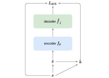
Figure 1: The process to compute the dCS loss in our scenario. Here, $\tilde{\bm{x}}$ is constructed from an original data $\bm{x}$. The estimator $\hat{k}$ for a weight $k$ in the dCS is computed via $\bm{x}$ and $\tilde{\bm{x}}$.

3.1 Preliminary

In our scenario, we have an unlabeled set $\mathcal{D}=\{\bm{x}^{(i)}\}_{i=1}^{n}$, where $n$ denotes the size of the set $\mathcal{D}$, and $\bm{x}^{(i)},i\in\{1,2,...,n\}$ are iid noisy data. Each $\bm{x}^{(i)}$ is sampled from a distribution that satisfies the following two assumptions (A1) and (A2).

1. Let us define $\bm{s}$ as clean data. Each sample is expressed by a feature vector. The dimension of each data is not necessarily the same. The dimension of $\bm{s}$ is denoted by ${\rm dim}(\bm{s})$.

2. For a fixed $\bm{s}\in\mathbb{R}^{{\rm dim}(\bm{s})}$, the noisy data $\bm{x}$ is expressed by $\bm{x}=\bm{s}+\bm{\epsilon}$, where $\bm{\epsilon}=(\epsilon_{1},..,\epsilon_{d},..,\epsilon_{\dim(\bm{s})})\in\mathbb{R}^{{\rm dim}(\bm{s})}$ is the noise vector. In addition, $\bm{\epsilon}$ has the isotropic distribution with zero mean, and the variance of each element is $\sigma^{2}$, i.e., the probability density is expressed as the function of $\|\bm{\epsilon}\|_{2}$ with $\mathbb{V}[\epsilon_{d}]=\sigma^{2}$ for all $d$. The noise intensity $\sigma$ can vary for each clean data $\bm{s}$.

The typical example of $\bm{\epsilon}$ satisfying (A2) is the multivariate normal distribution $\mathcal{N}_{D}(\bm{0},\sigma^{2}I_{D})$ with $D={\rm dim}(\bm{s})$. Under the above assumption, our goal is to propose an efficient loss function that can assist DRL.

Here, we review the mathematical definition of BSM:

Definition 1 (Blind-Spot Masking, Figure 3 of Krull et al. [37]).

Consider a Bernoulli random vector $\bm{b}=(b_{1},\ldots,b_{D})^{\top}\in\{0,1\}^{D}$, where ${\rm Pr}(b_{d}=1)=\rho\in[0,1]$. Let $d_{i},i=1,...,\|\bm{b}\|_{1}$ denote an index satisfying $b_{d_{i}}=1$, where $d_{1}<,...,<d_{\|\bm{b}\|_{1}}$. Then, for each $d_{i}$-th ($i=1,...,\|\bm{b}\|_{1}$) pixel of a fixed noisy image $\bm{x}\in\mathbb{R}^{D}$, replace the $d_{i}$-th pixel with the random neighbor pixel. Here, the neighbor region of $d_{i}$-th pixel is defined as the mini-patch, whose center is the $d_{i}$-th pixel.

Additionally, we review the mathematical definition of $\tau$-AMN in Definition 3.

Definition 2 (Random subset $\tau$, Definition 1 of Sanada et al. [55]).

Assume $b_{t}$, $t\in\{1,2,...,T\}$ are iid random variables, and $b_{t}$ has the Bernoulli distribution with $p(b_{t}=1)=\rho\in(0,1]$. Let $\tau$ denote a random subset of $\{1,2,...,T\}$, and it is constructed by the following two steps:

1. Generate a Bernoulli vector $\bm{b}=(b_{1},b_{2},...,b_{T})^{\top}$.

2. Set $\emptyset$ as $\tau$, and repeat below for all $t\in\{1,2,...,T\}$: if $b_{t}=1$ then $\tau\leftarrow\tau\cup\{t\}$. Otherwise, $\tau\leftarrow\tau$.

Definition 3 ($\tau$-AMN, Definition 1 of Sanada et al. [55]).

Let $\bm{x}\in\mathbb{R}^{T}$ denote a noisy speech data, and $x_{t}$ denote its $t$-th element. For $t\in\{1,2,...,T\}$, we define a time interval $\mathcal{I}_{t}$ by $\mathcal{I}_{t}=\left\{q\in\mathbb{N}\mid q\in[t-\Delta,t+\Delta]\setminus\{t\}\right\}$, where $\Delta\in\mathbb{N}$ is fixed for all $t$. Then, based on $\bm{x}$, another noisy speech data $\tilde{\bm{x}}\in\mathbb{R}^{T}$ is constructed by $\tau$-AMN, whose procedure is as follows:

1. Generate a random subset $\tau\subseteq\{1,2,...,T\}$ as described in Definition 2, and set an arbitrary $T$ dimensional vector as $\tilde{\bm{x}}$.

2. Repeat the procedure below for all $t\in\{1,2,...,T\}$: if $t\in\tau$, sample $t^{\prime}$ from $\mathcal{I}_{t}$ at random, and then $\tilde{x}_{t}\leftarrow x_{t^{\prime}}$. Otherwise, $\tilde{x}_{t}\leftarrow x_{t}$.

We refer to $\tilde{\bm{x}}$ as the masked $\bm{x}$.

3.2 Theory behind dCS Loss

In this section, we show a theoretical background of our approach. Given a noisy data $\tilde{\bm{x}}$ and the clean data $\bm{s}$, ideally we aim at minimizing the supervised loss $\mathbb{E}_{\bm{s},\tilde{\bm{\epsilon}}}\left[\ell_{\mathrm{CS}}\left(\hat{\bm{s}},\bm{s}\right)\right]$, where $\hat{\bm{s}}=h_{\theta}(\tilde{\bm{x}})$ is the output of an AE $h_{\theta}$, and $\theta$ is a set of trainable parameters. For $\ell_{\rm CS}$, see Eq.(1). However, the estimation using the supervised loss is not feasible, since 1) the clean data $\bm{s}$ is not available, and 2) we can access only single noisy data $\bm{x}$. This section is devoted to provide a way to circumvent these difficulties.

Let us consider the assumption for a pair of two noisy data $(\bm{x},\tilde{\bm{x}})$.

1. For a fixed $\bm{s}\in\mathbb{R}^{{\rm dim}(\bm{s})}$, $\bm{x}$ and $\tilde{\bm{x}}$ are expressed by $\bm{x}=\bm{s}+\bm{\epsilon}$ and $\tilde{\bm{x}}=\bm{s}+\tilde{\bm{\epsilon}}$ respectively, where $\bm{\epsilon},\tilde{\bm{\epsilon}}\in\mathbb{R}^{{\rm dim}(\bm{s})}$ are independent random vectors. The noise vectors, $\bm{\epsilon}$ and $\widetilde{\bm{\epsilon}}$, satisfy (A2).

In Section 3.4, we show how to imitate the situation of (A3) using a single noisy data $\bm{x}$. In addition, under the assumption (A2) with $D=\dim(\bm{s})$, let us define the function $k_{D,\sigma}(t),\,t\geq 0$ by the expectation

$$k_{D,\sigma}(t)=\mathbb{E}_{\bm{\epsilon}}\bigg{[}\frac{\epsilon_{1}+t}{\|\bm{\epsilon}+t\bm{e}_{1}\|_{2}}\bigg{]}$$ (3)

for ${\bm{e}}_{1}=(1,0,\ldots,0)^{\top}\in\mathbb{R}^{D}$.

Theorem 1.

Assume (A1) and (A3). Consider a fixed clean data $\bm{s}$, and let $D$ denote the dimension of $\bm{s}$. Fix the Bernoulli vector $\bm{b}=(b_{1},\ldots,b_{D})^{\top}\in\{0,1\}^{D}$. Let $(\bm{x},\tilde{\bm{x}})$ be a pair of two random noisy data satisfying (A3). Let $h_{\theta}:\mathbb{R}^{D}\to\mathbb{R}^{D},\bm{x}\mapsto h_{\theta}(\bm{x})$ be a function parameterized by $\theta$. Then, the following holds:

$$\mathbb{E}_{\tilde{\bm{\epsilon}}}\left[\ell_{\rm CS}(\bm{b}\odot\bm{s},\bm{b}\odot\hat{\bm{s}})|\bm{s},\bm{b}\right]\!=\!\frac{\mathbb{E}_{\bm{\epsilon},\tilde{\bm{\epsilon}}}\left[\ell_{\rm CS}(\bm{b}\odot\bm{x},\bm{b}\odot\hat{\bm{s}})|\bm{s},\bm{b}\right]}{k_{\|\bm{b}\|_{1},\sigma}\left(\|\bm{b}\odot\bm{s}\|_{2}\right)},$$ (4)

where $\odot$ denotes Hadamard product, and $\hat{\bm{s}}=h_{\theta}\left(\tilde{\bm{x}}\right)$. The definition of $\ell_{\rm CS}$ is shown in Eq.(1), and the weight function $k_{\|\bm{b}\|_{1},\sigma}$ is given by Eq.(3) with the $\|\bm{b}\|_{1}$-dimensional marginal distribution of $\bm{\epsilon}$.

The proof is shown in Appendix C.1.

We consider the parameter learning in unsupervised scenario. Let $\theta^{\ast}$ be a minimizer of $\mathbb{E}_{\bm{s},\tilde{\bm{\epsilon}},\bm{b}}\left[\ell_{\rm CS}(\bm{b}\odot\bm{s},\bm{b}\odot\hat{\bm{s}})\right]$. Once $k_{\|\bm{b}\|_{1},\sigma}\left(\|\bm{b}\odot\bm{s}\|_{2}\right)$ is computed, Eq.(4) enables us to obtain $\theta^{\ast}$ by minimizing

$$\mathbb{E}_{\bm{s},\bm{b}}\left[\frac{\mathbb{E}_{\bm{\epsilon},\tilde{\bm{\epsilon}}}\left[\ell_{\rm CS}(\bm{b}\odot\bm{x},\bm{b}\odot\hat{\bm{s}})|\bm{s},\bm{b}\right]}{k_{\|\bm{b}\|_{1},\sigma}\left(\|\bm{b}\odot\bm{s}\|_{2}\right)}\right].$$ (5)

In Section 3.3, we show an estimator of $k_{\|\bm{b}\|_{1},\sigma}\left(\|\bm{b}\odot\bm{s}\|_{2}\right)$ using $\bm{x}$ and $\tilde{\bm{x}}$.

Since the clean data $\bm{s}$ is unknown, direct minimization of the supervised loss is not feasible. However, Proposition 1 below implies that the minimization of Eq.(5) can also contribute to minimizing the supervised loss tightly. To this end, let us introduce the following condition:

1. The range of each random variable $\tilde{\bm{x}}$, $\bm{s}$, denoted by $\mathcal{X}$ and $\mathcal{Y}$ respectively, is compact subset of $\mathbb{R}^{D}\backslash\{\mathbf{0}\}$. Moreover, $h_{\theta}$ is continuous on $\mathcal{X}$, and the Euclidean norm of the vector $\hat{\bm{s}}=h_{\theta}(\tilde{\bm{x}})$ is positive for every $\tilde{\bm{x}}\in\mathcal{X}$.

Proposition 1.

Assume the condition (A4) holds. Suppose that the probability $\rho$ in Definition 1 satisfies $\rho\in(0,1)$. Then, the following inequality holds for each parameter $\theta$:

$$\mathbb{E}_{\bm{s},\bm{b}}\left[\mathbb{E}_{\tilde{\bm{\epsilon}}}\left[\ell_{\mathrm{CS}}\left(\bm{b}\odot\hat{\bm{s}},\bm{b}\odot\bm{s}\right)|\bm{s},\bm{b}\right]\right]=\Theta(\mathbb{E}_{\bm{s},\tilde{\bm{\epsilon}}}\left[\ell_{\mathrm{CS}}\left(\hat{\bm{s}},\bm{s}\right)\right]),$$ (6)

where $a=\Theta(b)$ means that there exist some $M_{1}\leq M_{2}$ such that $M_{1}b\leq a\leq M_{2}b$.

The proof is given in Appendix C.2. Note that it is a natural idea that the minimization of the left hand in Eq.(6) can contribute to minimizing the supervised loss $\mathbb{E}_{\bm{s},\tilde{\bm{\epsilon}}}\left[\ell_{\mathrm{CS}}\left(\hat{\bm{s}},\bm{s}\right)\right]$. Intuitively, if the misalignment of the directions of the vectors $\hat{\bm{s}}\odot\bm{b}$ and $\bm{s}\odot\bm{b}$ for a Bernoulli random vector $\bm{b}$ is reduced sufficiently, then the directions of $\bm{s}$ and $\hat{\bm{s}}$ should probably be the same.

Remark 1.

Assumption (A4) can be relaxed. Indeed, the cosine similarity function $\ell_{\mathrm{CS}}$ is usually defined as $\ell_{\mathrm{CS}}(\bm{u},\bm{v})=-\langle\bm{u},\bm{v}\rangle/\max\{\|\bm{u}\|_{2}\|\bm{v}\|_{2},\eta\}$, where $\eta>0$ is a sufficiently small value (e.g., PyTorch [49] supports the class torch.nn.CosineSimilarity with such a small value, where the default one is set $1.0\times 10^{-8}$ [60]). Using this practical definition, these assumptions can be replaced with the conditions that both $h_{\theta}(\mathcal{X})$ and $\mathcal{Y}$ are bounded for any $\theta$.

3.3 Estimation of the Weight $k_{D,\sigma}$

Let us consider how to estimate $k_{D,\sigma}(\|\bm{s}\|_{2})$ from the $D$-dimensional paired data $(\bm{x},\tilde{\bm{x}})$. We assume the following assumptions to evaluate the estimation accuracy.

1. The distribution of $\bm{\epsilon}$ and $\widetilde{\bm{\epsilon}}$ is sub-Gaussian, $\bm{\epsilon},\widetilde{\bm{\epsilon}}\sim\mathrm{subG}(\bar{\sigma}^{2})$, where $\sigma^{2}\leq\bar{\sigma}^{2}$,

2. The distribution of the centered random variables, $\|\bm{\epsilon}\|_{2}^{2}-D\sigma^{2}$ and $\|\widetilde{\bm{\epsilon}}\|_{2}^{2}-D\sigma^{2}$, are sub-exponential $\mathrm{subE}(4\bar{\sigma}^{4}D,4\bar{\sigma}^{2})$.

The definition of the sub-Gaussian and sub-exponential is shown in Appendix C.3. To be exact, (A5) and (A6) are assumptions for the sequence of distributions indexed by $D$. In general, each element of $\bm{\epsilon}$ is not independent each other under the isotropic distribution. When $\bm{\epsilon}$ and $\widetilde{\bm{\epsilon}}$ are both the multivariate normal distribution $\mathcal{N}_{D}(\bm{0},\sigma^{2}I_{D})$, (A5) and (A6) are satisfied with $\bar{\sigma}^{2}=\sigma^{2}$.

Remark 2.

Let us consider a sufficient condition of (A5) and (A6). Let $\psi_{D,s}$ be the probability density of $\mathcal{N}_{D}(\bm{0},s^{2}I_{D})$ and $G_{D}$ be a distribution function on the set of positive numbers. Suppose that the isotropic probability density of $\bm{\epsilon}$ and $\widetilde{\bm{\epsilon}}$ is expressed by $\int\psi_{D,s}(\bm{\epsilon})G_{D}(ds)$ [17]. Then, (A5) and (A6) hold for a large $\bar{\sigma}^{2}$ when i) $S\sim G_{D}$ is uniformly bounded for any $D$, ii) $\mathbb{E}[S^{2}]=\sigma^{2}$, and iii) $\sqrt{D}(S^{2}-\sigma^{2})$ has a sub-Gaussian distribution with the parameter independent of $D$. Note that $\bm{\epsilon}\sim\mathcal{N}_{D}(\bm{0},\sigma^{2}I_{D})$ corresponds to $G_{D}$ such that $P(S=\sigma)=1$.

We show an approximate calculation of $k_{D,\sigma}$. Let us consider the decomposition, $\bm{\epsilon}=r\bm{u}$, where $\bm{u}$ is the unit vector and $r=\|\bm{\epsilon}\|_{2}$ is the length of $\bm{\epsilon}$. Since $\bm{\epsilon}$ is isotropic, $\bm{u}$ is uniformly distributed on the unit sphere and the length $r$ is independent of $\bm{u}$. For $c=\|\bm{s}\|_{2}/\sigma\sqrt{D}$, Eq.(3) leads to

$$k_{D,\sigma}(\|\bm{s}\|_{2})=\mathbb{E}_{r,\bm{u}}\left[\frac{ru_{1}/\sqrt{D}+c}{\|r\bm{u}/\sqrt{D}+c\bm{e}_{1}\|_{2}}\right],$$ (7)

where $\bm{u}=(u_{1},\ldots,u_{D})$ is the unit vector uniformly distributed on $D-1$ dimensional unit sphere and $r$ is the positive random variable such that $\mathbb{V}[ru_{1}]=1$. Once an estimator of $c$ is obtained, $k_{D,\sigma}(\|\bm{s}\|_{2})$ is estimated by the Monte Carlo approximation. The sampling of $\bm{u}$ is given by the normalized vector of the multivariate normal distribution $\mathcal{N}_{D}(\bm{0},I_{D})$. For the sampling of one-dimensional random variable $r$, a number of efficient methods are available.

When $\bm{\epsilon}$ has the multivariate normal distribution, $\mathcal{N}_{D}(\bm{0},\sigma^{2}I_{D})$, the Monte Carlo approximation becomes simpler. Let $\kappa$ and $\nu$ be independent random variables such that $\kappa\sim\mathcal{N}(0,1)$ and $\nu\sim\chi_{D-1}^{2}$, where $\chi_{D-1}^{2}$ is the chi-square distribution with the degree of freedom $D-1$. Then, a brief calculation yields that

$$k_{D,\sigma}(\|\bm{s}\|_{2})=\mathbb{E}_{\kappa,\nu}\left[\frac{\kappa/\sqrt{D}+c}{\sqrt{(\kappa/\sqrt{D}+c)^{2}+\nu/D}}\right].$$

The sampling of two random variables, $\kappa$ and $\nu$, provides an accurate Monte Carlo approximation for the expectation.

We show a simple estimate of $c=\|\bm{s}\|_{2}/\sigma\sqrt{D}$ using the paired data $\bm{x},\tilde{\bm{x}}$. The assumptions on $\bm{x}$ and $\tilde{\bm{x}}$ leads to $\mathbb{E}[\bm{x}^{\top}\tilde{\bm{x}}]=\|\bm{s}\|_{2}^{2}$, and $\mathbb{E}[\|\bm{x}-\tilde{\bm{x}}\|_{2}^{2}]=2D\sigma^{2}$. Hence, we have $\frac{\|\bm{s}\|_{2}}{\sigma\sqrt{D}}=\sqrt{\frac{2\mathbb{E}[\bm{x}^{\top}\tilde{\bm{x}}]}{\mathbb{E}[\|\bm{x}-\tilde{\bm{x}}\|_{2}^{2}]}}$. As a naive estimate of $\|\bm{s}\|_{2}/\sigma\sqrt{D}$ using only the pair $(\bm{x},\tilde{\bm{x}})$, we propose the estimator $\widehat{c}=\sqrt{2\max\{\bm{x}^{\top}\tilde{\bm{x}},0\}/\|\bm{x}-\tilde{\bm{x}}\|_{2}^{2}}$. Since the expectation, $\mathbb{E}[\bm{x}^{\top}\tilde{\bm{x}}]=\|\bm{s}\|_{2}^{2}$, is positive, the cut-off at $0$ is introduced in the estimator.

As a result, the estimator of $k_{D,\sigma}(\|\bm{s}\|_{2})$ is constructed via the following two steps:

1. Compute $\widehat{c}=\frac{\sqrt{2\left[\bm{x}^{\top}\tilde{\bm{x}}\right]_{+}}}{\left\|\bm{x}-\tilde{\bm{x}}\right\|_{2}}$, where $[a]_{+}=\max\{a,0\}$.

2. Compute the Monte Carlo approximation of the right-hand side of Eq.(7) with $\widehat{c}$ instead of $c$.

When the probability density of $\bm{\epsilon}$ and $\widetilde{\bm{\epsilon}}$ is $\mathcal{N}_{D}(\bm{0},\sigma^{2}I)$, the estimator of the weight function is expressed by

$$\hat{k}_{D,\sigma}(\|\bm{s}\|_{2})=\frac{1}{n_{s}}\sum_{i=1}^{n_{s}}\frac{\widehat{c}+\frac{\kappa_{i}}{\sqrt{D}}}{\sqrt{\left(\widehat{c}+\frac{\kappa_{i}}{\sqrt{D}}\right)^{2}+\frac{\nu_{i}}{D}}},$$ (8)

where $\{\kappa_{i}\}_{i=1}^{n_{s}}$ and $\{\nu_{i}\}_{i=1}^{n_{s}}$ are iid samples from $\mathcal{N}(0,1)$ and $\chi_{D-1}^{2}$ respectively.

Let us evaluate the statistical accuracy of the estimator $\widehat{c}$ to the SN-ratio $c=\|\bm{s}\|_{2}/\sigma\sqrt{D}$. For a finite $D$, we derive an upper bound of the error $|c-\widehat{c}|$. Also, we see that the error converges to zero as $D$ goes to infinity if the SN-ratio, $c$, is not extremely small.

Theorem 2.

Assume (A3), (A5), and (A6). Then, there exists $\delta_{c}$ and $D_{c,\bar{\sigma}^{2},\sigma^{2},\delta}$ such that for $\delta\in(0,\delta_{c})$ and $D\geq D_{c,\bar{\sigma}^{2},\sigma^{2},\delta}$, the inequality

$$|c-\widehat{c}|\leq 12\frac{\bar{\sigma}^{2}}{\sigma^{2}}\bigg{(}c+\frac{1}{c}\bigg{)}\frac{\log(12/\delta)}{\sqrt{D}}$$

holds with probability greater than $1-\delta$.

The proof is shown in Appendix C.3. For $c^{2}$ less than $26$, $\delta$ can take any value in the interval $(0,\,0.01)$. When the order of $c$ is greater than $D^{-1/4}$, it holds that $D_{c,\bar{\sigma}^{2},\sigma^{2},\delta}=o(D)$. The explicit expressions of $\delta_{c}$ and $D_{c,\bar{\sigma}^{2},\sigma^{2},\delta}$ are presented in the proof.

Let us consider the asymptotic property of the estimator.

• Suppose $c=\frac{\|\bm{s}\|_{2}}{\sigma\sqrt{D}}\rightarrow 0$ and $\|\bm{s}\|_{2}/D^{1/4}\rightarrow\infty$ for $\bm{s}\in\mathbb{R}^{D}$ as $D\rightarrow\infty$. In this case, $c$ is greater than the order of $D^{-1/4}$ and the condition on $D$ is asymptotically satisfied. The estimation error, $|c-\widehat{c}|$, is bounded above by $o_{p}(D^{-1/4})$.

• Suppose $c=\frac{\|\bm{s}\|_{2}}{\sigma\sqrt{D}}\rightarrow c_{\infty}\in(0,\infty)$ as $D\rightarrow\infty$. Then, we have $|c-\widehat{c}|=O_{p}(D^{-1/2})$ and $|c_{\infty}-\widehat{c}|\leq|c_{\infty}-c|+O_{p}(D^{-1/2})$. We see that $\widehat{c}\rightarrow c_{\infty}$ holds in probability.

The above analysis means that if the average intensity of the pixel-wise signal, $\|\bm{s}\|_{2}/\sqrt{D}$, is not ignorable in comparison to $\sigma$, i.e., the order of $\|\bm{s}\|_{2}$ is greater than $D^{1/4}$ for $\bm{s}\in\mathbb{R}^{D}$, one can accurately estimate the SN ratio $c$ using $\widehat{c}$.

The following theorem ensures that an approximation of $k_{D,\sigma}(\|\bm{s}\|_{2})$ for large $D$ does not require the Monte Carlo sampling.

Theorem 3.

Assume (A3), (A5), and (A6). Then, it holds that $k_{D,\sigma}(\|\bm{s}\|_{2})=\frac{c}{\sqrt{c^{2}+1}}+O(D^{-1/2})$ for large $D$.

The proof is shown in Appendix C.3. From Theorem 3 and Theorem 2, we have $\widehat{c}/\sqrt{\widehat{c}^{2}+1}=k_{D,\sigma}(\|\bm{s}\|_{2})+O_{p}(D^{-1/2})$.

3.4 Definition of dCS Loss

From Theorem 1, the proposed dCS loss with the noisy data $\bm{x}$ is given by

$$\ell_{\rm dCS}\left(\bm{x}\right)=\mathbb{E}_{\bm{b}}\left[\frac{\ell_{\rm CS}(\bm{b}\odot\bm{x},\bm{b}\odot h_{\theta}\left(\tilde{\bm{x}}\right))}{\hat{k}_{\|\bm{b}\|_{1},\sigma}\left(\|\bm{b}\odot\bm{s}\|_{2}\right)}\right],$$ (9)

where $\tilde{\bm{x}}$ is constructed from $\bm{x}$, $\bm{b}$, and domain specific masking technique (e.g., BSM of Definition 1 for the vision domain and $\tau$-AMN of Definition 3 for speech). In addition, $\hat{k}_{\|\bm{b}\|_{1},\sigma}\left(\|\bm{b}\odot\bm{s}\|_{2}\right)$ is computed without knowing $\bm{s}$; see Eq.(8). Furthermore, the empirical risk for dCS over $\mathcal{D}$ is given by

$$L_{\rm dCS}(\theta)=\frac{1}{n}\sum_{i=1}^{n}\ell_{\rm dCS}(\bm{x}^{(i)}).$$ (10)

For a mini-batch $\mathcal{B}\subseteq\mathcal{D}$, we compute $L_{\rm dCS}$ as described in Algorithm 1, which is constructed under the Gaussian assumption.

Remark 3.

An approximation of $\hat{k}_{\|\bm{b}\|_{1},\sigma}\left(\|\bm{b}\odot\bm{s}\|_{2}\right)$ leads to $\ell_{\rm dCS}(\bm{x})=\frac{\sqrt{\hat{c}_{\bm{x}}^{2}+1}}{\hat{c}_{\bm{x}}+\eta}\ell_{\mathrm{CS}}(\bm{b}\odot\bm{x},\bm{b}\odot h_{\theta}(\tilde{\bm{x}}))$, where $\hat{c}_{\bm{x}}=\frac{\sqrt{2[(\bm{b}\odot\bm{x})^{T}(\bm{b}\odot\tilde{\bm{x}})]_{+}}}{\|\bm{b}\odot\bm{x}-\bm{b}\odot\tilde{\bm{x}}\|_{2}}$ and $\eta$ is a small positive constant. In Algorithm 1, however, we propose the loss function based on Monte Carlo sampling defined from Eq.(8) and (9) in order to deal with data with not only a large $D$ but a small $D$.

Algorithm 1 : Computation of $L_{\rm dCS}$ for a mini-batch $\mathcal{B}$

1:Input Mini-batch (a subset of unlabeled noisy dataset $\mathcal{D}$): $\mathcal{B}=\left\{\bm{x}^{(i)}\right\}_{i=1}^{m}$ , AutoEncoder: $h_{\theta}$, Mean of Bernoulli distribution: $\rho\in[0,1]$.

2:Output Empirical dCS risk for $\mathcal{B}$.

3:for $i=1,\cdots,m$ do

4:     

Generate a Bernoulli vector $\bm{b}^{(i)}\in\{0,1\}^{\textrm{dim}\left(\bm{x}^{(i)}\right)}$ based on $\rho$. Then, construct another noisy data $\tilde{\bm{x}}^{(i)}$ by using $\bm{x}^{(i)}$, $\bm{b}^{(i)}$, and domain-specific masking technique, such as BSM of Definition 1 and $\tau$-AMN of Definition 3.

5:     

Using $\bm{x}^{(i)}$, $\bm{b}^{(i)}$, $\tilde{\bm{x}}^{(i)}$, and Eq.(8), compute the following estimated weight in Eq.(9): $\hat{k}_{\|\bm{b}^{(i)}\|_{1},\sigma}\left(\left\|\bm{b}^{(i)}\odot\bm{s}^{(i)}\right\|_{2}\right)$, where $\bm{s}^{(i)}$ means the clean data of $\bm{x}^{(i)}$ and $\tilde{\bm{x}}^{(i)}$.

6:Compute $L_{\rm dCS}$ of Eq.(10) for $\mathcal{B}$ by

$$\frac{1}{m}\sum_{i=1}^{m}\frac{\ell_{\rm CS}\left(\bm{b}^{(i)}\odot\bm{x}^{(i)},\bm{b}^{(i)}\odot h_{\theta}\left(\tilde{\bm{x}}^{(i)}\right)\right)}{\hat{k}_{\|\bm{b}^{(i)}\|_{1},\sigma}\left(\left\|\bm{b}^{(i)}\odot\bm{s}^{(i)}\right\|_{2}\right)}.$$

Remark 4.

Suppose that we use a small $\rho$ (mean of Bernoulli distribution), say $\rho=0.1$, for a domain-specific masking technique such as blind-spot masking. Let $\bm{\epsilon}^{(i)}$ and $\tilde{\bm{\epsilon}}^{(i)}$ be the noise to the data. One can observe that the correlation between $\bm{b}\odot\bm{\epsilon}^{(i)}$ and $\bm{b}\odot\tilde{\bm{\epsilon}}^{(i)}$ is weakened by using $\bm{b}$ with a small $\rho$. Under this condition, the formula in Theorem 1 will hold approximately. Furthermore, small $\rho$ makes the computation of Eq.(9) efficient. On the other hand, if $\rho$ is close to one, their correlation remains. A choice of $\rho$ is important in practice.

4 NUMERICAL EXPERIMENTS

In this section, we evaluate our dCS loss on multiple DRL settings. We conduct four kinds of experiments: Expt0, Expt1, Expt2, and Expt3, where we focus on the vision domain in Expt0, Expt1, and Expt2 and the speech domain in Expt3. Throughout this section, for a vision dataset (resp. for a speech dataset), we compute the dCS loss via Algorithm 1 with BSM of Definition 1 (resp. with $\tau$-AMN of Definition 3). Regarding the evaluation, we employ 1) the test accuracy (%) of linear evaluation protocol [7] and 2) the clustering accuracy (%) of clustering protocol [45]; see Section 4.1. For the environmental setups and details of the hyper-parameters used in our experiments, see Appendix D.3 and Appendix D.4 respectively.

4.1 Evaluation Protocol

In this subsection, a set of the features and the corresponding true label set for training are denoted by $\mathcal{D}$ and $\bm{y}$. Similarly, a set of the features and the corresponding true label set for testing are denoted by $\mathcal{D}_{\rm tst}$ and $\bm{y}_{\rm tst}$. Let $f_{\psi}$ be an encoder with a set of trainable parameters $\psi$. The trained set is defined by $\psi^{\ast}$.

1) Linear Evaluation Protocol [7]

We follow the standard evaluation protocol of self-supervised representation learning [7]: at first, train an encoder $f_{\psi}$ using $\mathcal{D}$. After the training, freeze the trained parameters of the encoder, then attach a trainable linear head. After that, train the linear head using $\mathcal{D}$ and $\bm{y}$. At last, using the trained encoder and the trained linear-head, compute the test accuracy (%) for $\mathcal{D}_{\rm tst}$ and $\bm{y}_{\rm tst}$.

2) Clustering Protocol [45]

We follow the evaluation protocol introduced by McConville et al. [45]. For convenience, we call this protocol clustering protocol. For completeness, we overview the evaluation protocol based on McConville et al. [45]. Let $\tilde{\mathcal{D}}=\mathcal{D}\cup\mathcal{D}_{\rm tst}$ and $\tilde{\bm{y}}=\bm{y}\cup\bm{y}_{\rm tst}$, where $|\tilde{\mathcal{D}}|=\tilde{n}$. Let $\bm{x}^{(i)}$ (resp. $y^{(i)}$) denote the $i$-th data point in $\tilde{\mathcal{D}}$ (resp. true label of $\bm{x}^{(i)}$ in $\tilde{\bm{y}}$). In this protocol, firstly, train an encoder $f_{\psi}$ for the dataset $\tilde{\mathcal{D}}$. After the training, compute $\bm{z}^{(i)}=f_{\psi^{\ast}}(\bm{x}^{(i)})$. Then, use UMAP [46] to transform $\{\bm{z}^{(i)}\}_{i=1}^{\tilde{n}}$ into $C$-dimensional feature vectors, where $C$ is the number of classes. After this, perform Gaussian Mixture Model Clustering (GMMC) [12] on the transformed feature vectors to estimate cluster labels. Here, $C$ is set as the number of components in GMMC. At last, compute the clustering accuracy (%) as follows:

$$100\times\max_{\iota}\frac{\sum_{i=1}^{\tilde{n}}\mathbb{I}\left[y^{(i)}=\iota\left(\hat{y}^{(i)}\right)\right]}{\tilde{n}},$$

where $\hat{y}^{(i)},i=1,...,\tilde{n}$ denote the estimated cluster labels, $\iota$ is a permutation of cluster labels, and $\mathbb{I}[\;\cdot\;]$ is the indicator function. Note that for the computation of the best permutation of the cluster labels, following the standard approach of Yang et al. [67], we use the Kuhn-Munkres algorithm [38].

4.2 Expt0: Performance Evaluation for Gaussian Noise on Vision Dataset, using AutoEncoder

In Expt0, using an AE, we evaluate the performance of the dCS when the noise on a dataset satisfies the assumption (A2) of Section 3.1, while comparing it with baseline methods.

4.2.1 Setting in Expt0

We construct Noisy-MNIST from the original MNIST [40]. Let $\bm{x}$ denote an image in MNIST, whose pixels are normalized within $[0,1]$ range. Then, the noisy MNIST image is defined as $\bm{x}+\bm{\epsilon}$, where $\bm{\epsilon}\sim\mathcal{N}(\bm{0},\sigma^{2}I)$ with $\sigma=0.01,0.1,0.3,0.5,\;\text{and}\;0.7$.

Let $h_{\theta}$ denote an MLP-based AE, whose encoder and decoder are $f_{\psi}$ and $\tilde{f}_{\zeta}$, respectively (i.e., $h_{\theta}=\tilde{f}_{\zeta}\circ f_{\psi}$). Let $\theta:=\psi\cup\zeta$ be a set of trainable parameters in the AE. We employ the common structure $D$-500-500-2000-$C$ for the encoder $f_{\psi}$ as McConville et al. [45] do, where $D$ and $C$ denote the dimension of data and the number of classes, respectively. Note that using the $f_{\psi}$, the structure of the AE $h_{\theta}$ is $D$-500-500-2000-$C$-2000-500-500-$D$; $D=784,C=10$ for Noisy-MNIST.

In this experiment, using Noisy-MNIST, we compare 1) MSE, 2) CS loss, 3) N2V loss, 4) SURE loss, and 5) dCS loss. Let $\mathcal{D}=\{\bm{x}^{(i)}\}_{i=1}^{n},\bm{x}^{(i)}\in\mathbb{R}^{D}$ be Noisy-MNIST. The objectives with 1) MSE and 2) the CS loss are defined respectively as follows:

$$\arg\min_{\theta}\frac{1}{n}\sum_{i=1}^{n}\left\|\bm{x}^{(i)}-h_{\theta}\left(\bm{x}^{(i)}\right)\right\|_{2}^{2}\;\text{and}\;\arg\min_{\theta}\frac{1}{n}\sum_{i=1}^{n}\ell_{\rm CS}\left(\bm{x}^{(i)},h_{\theta}\left(\bm{x}^{(i)}\right)\right),$$

where $\ell_{\rm CS}$ is given in Eq.(1). In addition, the objectives with 3) N2V loss, 4) SURE loss, and 5) dCS loss are defined as Eq.(10) of Krull et al. [37] (see also Eq.(11)), Eq.(6) of Zhussip et al. [71] ($\sigma$ is estimated using Chen et al. [6]), and Eq.(10), respectively. For details of the hyper-parameters, see Appendix D.3.

The comparing procedure is as follows: Firstly, using Noisy-MNIST and each loss, train the AE $h_{\theta}$ with the Adam optimizer [34] for eight hundred epochs. Secondly, evaluate the trained encoder by linear evaluation protocol and clustering protocol.

Table 1: Results on Expt0. The row with "Clustering" (resp. "Linear Evaluation") shows mean clustering accuracy (%) with std over twenty trials under clustering protocol (resp. mean test accuracy (%) with std over ten trials under linear evaluation protocol). The bold (resp. underlined) number means the best (resp. the second-best) accuracy.

Noise level (Protocol) $\backslash$ Loss	MSE	CS	N2V	SURE	dCS (Ours)
$\sigma=0.01$ (Clustering)	$96.83\pm 2.74$	$95.13\pm 4.83$	$93.12\pm 5.75$	$89.24\pm 6.48$	$96.27\pm 4.15$
$\sigma=0.01$ (Linear Evaluation)	$94.67\pm 0.25$	$94.11\pm 0.33$	$92.96\pm 0.51$	$82.15\pm 2.63$	$94.89\pm 0.29$
$\sigma=0.1$ (Clustering)	$97.21\pm 0.14$	$96.45\pm 2.92$	$92.20\pm 6.08$	$90.73\pm 7.15$	$94.96\pm 5.23$
$\sigma=0.1$ (Linear Evaluation)	$93.63\pm 0.12$	$93.69\pm 0.13$	$91.88\pm 0.25$	$89.04\pm 0.25$	$94.73\pm 0.12$
$\sigma=0.3$ (Clustering)	$94.25\pm 3.38$	$94.45\pm 3.08$	$89.94\pm 6.13$	$83.28\pm 5.74$	$96.22\pm 2.91$
$\sigma=0.3$ (Linear Evaluation)	$89.07\pm 0.41$	$90.04\pm 0.35$	$88.48\pm 0.70$	$85.15\pm 0.57$	$92.99\pm 0.25$
$\sigma=0.5$ (Clustering)	$81.39\pm 4.00$	$76.05\pm 6.42$	$82.20\pm 7.19$	$74.86\pm 4.78$	$91.41\pm 5.47$
$\sigma=0.5$ (Linear Evaluation)	$82.86\pm 0.51$	$84.44\pm 0.72$	$85.22\pm 0.48$	$79.98\pm 0.57$	$89.13\pm 0.48$
$\sigma=0.7$ (Clustering)	$68.85\pm 4.63$	$59.64\pm 4.74$	$72.42\pm 5.51$	$66.72\pm 3.77$	$78.76\pm 4.91$
$\sigma=0.7$ (Linear Evaluation)	$75.88\pm 0.40$	$77.30\pm 0.99$	$80.15\pm 0.57$	$74.17\pm 0.69$	$82.03\pm 0.45$

4.2.2 Results and Discussion for Expt0

The results are shown in Table 1. In summary, the dCS loss outperforms the other losses except for the results under clustering protocol when $\sigma=0.01,0.1$ are employed. In more detail, when $\sigma=0.1,0.3$, except for the case under the clustering protocol with $\sigma=0.1$, the result of dCS in each case is the best among the five losses. Here, we note that the results of CS follow those of dCS in most of the cases when $\sigma=0.1,0.3$. This implies that CS loss can also deal with the noise when the level is relatively low. On the other hand, when $\sigma$ becomes larger, i.e., $\sigma=0.5,0.7$, CS degrades its performance (and CS is outperformed by N2V). Thus, in high-level noise settings, CS does not work efficiently. However, our dCS still performs the best among them when $\sigma=0.5,0.7$, indicating that the performance of dCS is robust against both small and large noise.

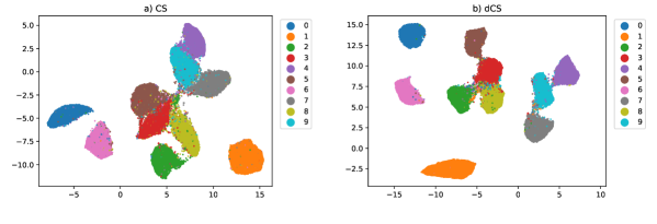
Figure 2: Two-dimensional UMAP visualization of the obtained representations on Noisy-MNIST with $\sigma=0.3$. The representation is the output of the trained encoder via minimizing a) CS loss and b) dCS loss. In both figures, the color expresses the class label ranging from zero to nine, as defined in the right side of each figure.

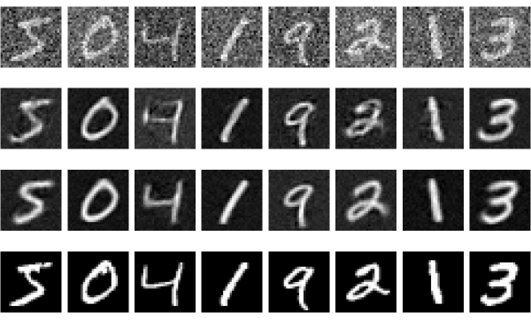
Figure 3: The first, second, third, and fourth row show images of Noisy-MNIST with $\sigma=0.3$, predicted corresponding clean images via the CS loss, predicted corresponding clean images via the dCS, and the corresponding clean images, respectively.

In Figure 2 of a) (resp. b)), using Noisy-MNIST with $\sigma=0.3$, the latent variables obtained by the trained encoder of the CS (resp. dCS) loss are visualized by UMAP [46]; for the details, see Appendix D.2. The figures show a clear improvement with the position of the clusters due to the denoising property of the dCS.

At last in Figure 3, using several images of Noisy-MNIST with $\sigma=0.3$, we show the predicted clean images from the corresponding Noisy-MNIST images via the dCS and CS, although our primary purpose in this study is to obtain a good representation of noisy data for downstream tasks. See Appendix D.2 for details of how to make the figure. The figure indicates 1) the dCS can remove the noise that satisfies (A2), and 2) the denoising ability of the dCS is better than that of the CS in general. Thus, the figure is consistent with our theory in Section 3.2.

4.3 Expt1: Performance Evaluation for Real-World Noise on Vision Dataset, using AutoEncoder

In Expt1, we conduct a similar experiment with Expt0 except for the condition that the noise may not satisfy (A2).

4.3.1 Setting in Expt1

Here, the following four datasets are employed: MNIST, USPS [30], Pendigits [1], and Fashion-MNIST [66]; see details of the datasets in Appendix D.1. For all four datasets, no additive noise is added: $\sigma=0$ for $\bm{\epsilon}\sim\mathcal{N}(\bm{0},\sigma^{2}I)$ of Section 4.2.1. We conduct almost the same experiment as Expt0 except for the difference in the dataset and removal of SURE loss.

Table 2: Results on Expt1. The row with "Clustering" (resp. "Linear Evaluation") shows mean clustering accuracy (%) with std over twenty trials under clustering protocol (resp. mean test accuracy (%) with std over ten trials under linear evaluation protocol). The bold (resp. underlined) number means the best (resp. the second-best) accuracy.

Dataset (Protocol) $\backslash$ Loss	MSE	CS	N2V	dCS (Ours)
MNIST (Clustering)	$96.78\pm 2.88$	$95.12\pm 4.86$	$93.28\pm 5.56$	$94.79\pm 5.45$
MNIST (Linear Evaluation)	$94.53\pm 0.33$	$94.09\pm 0.43$	$93.05\pm 0.33$	$95.07\pm 0.29$
USPS (Clustering)	$84.31\pm 6.49$	$85.24\pm 8.46$	$82.78\pm 10.2$	$86.94\pm 8.72$
USPS (Linear Evaluation)	$87.63\pm 0.47$	$87.19\pm 0.35$	$86.58\pm 0.51$	$88.08\pm 0.40$
Pendigits (Clustering)	$85.71\pm 3.89$	$85.84\pm 3.81$	$85.59\pm 2.99$	$82.22\pm 4.71$
Pendigits (Linear Evaluation)	$82.50\pm 1.21$	$82.82\pm 0.85$	$86.09\pm 1.89$	$81.84\pm 1.30$
Fashion-M (Clustering)	$60.70\pm 3.29$	$59.60\pm 3.79$	$60.66\pm 2.97$	$62.64\pm 4.50$
Fashion-M (Linear Evaluation)	$78.11\pm 0.56$	$75.53\pm 0.98$	$76.29\pm 0.69$	$76.70\pm 0.49$

4.3.2 Results and Discussion of Expt1

The results are shown in Table 2. In summary, our dCS performs the best since it achieves the four highest accuracies and one second-highest accuracy over the eight comparisons. This indicates that the dCS performs well even when the noise assumption (A2) is violated.

On the other hand, the dCS does not perform well for MNIST under clustering protocol. The result is consistent with the under-performing dCS results of $\sigma=0.01,0.1$ under clustering protocol in Table 1. In addition, the dCS does not perform well for Pendigits in both the protocols. A possible reason for the under-performing results with Pendigits is that BSM with the dCS does not work efficiently for low-dimensional data (the dimension of Pendigits data is only sixteen), unlike BSM with N2V.

At last, we investigate a possible reason why the results of linear evaluation are relatively insignificant compared to those of clustering in Table 2. Note that this tendency can be also seen in Table 1. The tendency could be caused by using true labels when training a linear classification head in the linear evaluation protocol. In the clustering protocol, no true label is used during training. In Expt0 and Expt1, the true labels possibly contribute to closing the performance gap between the dCS and baseline methods.

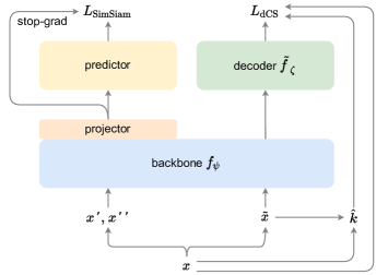
Figure 4: Architecture of SimSiam-dCS, where the dCS is being used as a regularizer in addition to the original SimSiam. The symbol $\bm{x}$ denotes raw data, while $\bm{x}^{\prime}$ and $\bm{x}^{\prime\prime}$ mean augmented data from $\bm{x}$. As for $\hat{k}$ and $\tilde{\bm{x}}$, their definitions are the same as those in Figure 1.

4.4 Expt2: Performance Evaluation for Real-World Noise on Vision Dataset, using SimSiam

In Expt2, we check how efficiently the dCS loss collaborates with SimSiam [8] as the regularizer. Here, the noise also may not satisfy (A2).

4.4.1 Setting in Expt2

We employ CIFAR10 [36], CIFAR100 [36], and Tiny-ImageNet [39]; see details in Appendix D.1. Similar to Expt1, no additive noise is added to all datasets.

We propose to incorporate our dCS objective into the SimSiam framework [8] by plugging a shallow decoder $\tilde{f}_{\zeta}$ to the end of backbone encoder $f_{\psi}$; see Figure 4. Hereafter we refer to this method as SimSiam-dCS. Let $h_{\theta}=\tilde{f}_{\zeta}\circ f_{\psi}$, where $\theta=\zeta\cup\psi$. Let us define an objective of SimSiam with a predictor MLP $g_{\xi}$ of Figure 4 by $L_{\rm SimSiam}(\psi,\xi)$; see Eq.(2). Then, the SimSiam-dCS objective is written as

$$L(\theta,\xi):=L_{\rm SimSiam}(\psi,\xi)+\lambda L_{\rm dCS}(\theta),$$

where $\lambda>0$ is a hyper-parameter controlling the balance between SimSiam and dCS objectives. Note that, following Chen and He [8], two augmented views $(\bm{x}^{\prime},\bm{x}^{\prime\prime})$ used for $L_{\rm SimSiam}$ are constructed from an original raw image $\bm{x}$. Besides, the blind-spot masked image (i.e., $\bm{\tilde{x}}$) used for $L_{\rm dCS}$ is also constructed from the same $\bm{x}$.

We also introduce two more variants of SimSiam, i.e., SimSiam-N2V, and SimSiam with BSM. In SimSiam-N2V, the N2V loss is a regularizer for SimSiam, like SimSiam-dCS. SimSiam with BSM is SimSiam with BSM added to the set of transformations with probability one.

For the backbone encoder $f_{\psi}$, following Chen and He [8], we have used the variant of ResNet-18 for CIFAR-10 [24] when running the experiments for CIFAR-10 and CIFAR-100 datasets. We also use a variant of ResNet-50 for Tiny-ImageNet. For the projection head [7], we use the two and three-layer MLPs for the ResNet-18 and ResNet-50 model, respectively, where we follow Chen and He [8] for the design of these MLPs. The decoder $\tilde{f}_{\zeta}$ is a single linear layer for CIFAR-10 and CIFAR-100, while a five-layer convolutional decoder with pixel shuffling [57] was used for Tiny-ImageNet. We followed the hyper-parameter setups of Chen and He [8], where the settings of ImageNet were used for Tiny-ImageNet. We have fixed $\lambda=0.01$ for CIFAR and $\lambda=0.02$ for Tiny-ImageNet.

We have used the official SimSiam package for reproducing the baseline and implementing SimSiam-dCS. See Appendix D.3 for further details of the hyper-parameters.

In this experiment, we compare 1) SimSiam, 2) SimSiam with BSM, 3) SimSiam-N2V, and 4) SimSiam-dCS. We follow the standard setting of Chen and He [8]: Firstly, train each DNN (Deep NN)-based model for eight hundred epochs. Then, the trained encoder (corresponding to the backbone of Figure 4) is evaluated by the linear evaluation protocol of Section 4.1.

In Expt2, only one trial is conducted for each method because of the high computing cost of SimSiam. Additionally, we did not employ the clustering protocol, since the output’s dimension of the backbone is too large to construct a meaningful k-nearest neighbor graph for UMAP. Moreover, we focus on only SimSiam here, because it is known to perform well even with small batch size, unlike SimCLR [7] and BYOL [22], which suffer from small batch size; see Section 2.2.

At last, we remark that the dCS regularizer can be a promising way to improve the performance of SimCLR and BYOL, since the two methods use the CS and a similar DNN to SimSiam.

4.4.2 Results and Discussion of Expt2

The results are shown in Table 3. In summary, our SimSiam-dCS performs the best for all datasets, and we observed some margin between them for CIFAR-100. In Table 4, we report the results of SimSiam-dCS with different $\lambda$. The table shows that the performance of SimSiam-dCS is robust against the change of $\lambda$.

Table 3: Results on Expt2. We report test-set accuracy (%) with one trial under linear evaluation protocol. The bold (resp. underlined) number means the best (resp. the second-best) accuracy.

Method $\backslash$ Dataset	CIFAR-10	CIFAR-100	Tiny-ImageNet
SimSiam (repro.)	$91.55$	$63.72$	$53.61$
SimSiam with BSM	$91.24$	$64.30$	$53.21$
SimSiam-N2V	$91.68$	$64.59$	$53.72$
SimSiam-dCS (Ours)	$91.73$	$65.20$	$53.77$

Table 4: Test accuracy (%) of SimSiam-dCS with different $\lambda$ values under linear evaluation protocol. The symbol "-" means that no result is available.

Dataset $\backslash$ $\lambda$	0.0001	0.001	0.01	0.02	0.05
CIFAR-10	$91.54$	$91.30$	$91.73$	-	$91.46$
CIFAR-100	$64.19$	$63.98$	$65.20$	-	$65.05$
Tiny-ImageNet	$53.37$	$53.58$	$52.71$	$53.77$	-

Remark 5.

The concurrent work by Baier et al. [2] proposes SidAE, which is a combination of the following two different RL methods: SimSiam [8] and a denoising AutoEncoder of Vincent et al. [63]. They aim to leverage the information that can be learned by one method to make up for the shortcomings of another. Although the motivation of the experiments presented in Section 4.4 in our work is similar to Baier et al. [2], we remark that the reconstruction loss used in SidAE is defined by the Euclidean norm. Also, Baier et al. [2] do not compare the performance of their proposed method to that of SimSiam with the CS loss. On the other hand, we propose a modified CS loss that can handle the noise in data and experimentally verify that SimSiam with the dCS regularizer can outperform SimSiam with the N2V regularizer, where the N2V regularizer is also defined by the Euclidean norm. Therefore, our work provides new insights that are not shown by Baier et al. [2].

4.5 Expt3: Performance Evaluation for Real-World Noise on Speech Dataset, using Large AutoEncoder

In Expt3, using a large AE, we evaluate the performance of the dCS when the noise on a speech dataset may not satisfy the assumption (A2).

4.5.1 Setting in Expt3

Using ESC-50 [50] dataset, we compare 1) MSE, 2) CS, 3) N2V, and 4) dCS. The dataset contains two thousand data samples with $220500$ dimension, and the number of classes is fifty. Inspired by the recent self-supervised learning methods [43, 21] that use the Transformer encoder [62] or its variants, we use an AE $h_{\theta}$ defined by Vision-Transformer (ViT) [15]. For further details on ESC-50, see Appendix D.1. We add no additive noise to the dataset.

The procedure for comparing the four losses is as follows: Firstly, using the training set (the size is sixteen hundred) and each loss, train the ViT-based AE for four thousand epochs. Secondly, evaluate the trained encoder by linear evaluation protocol using the test set (the size is four hundred). For computing the dCS loss, we use Algorithm 1 with $\tau$-AMN of Definition 3. The loss of N2V is also defined via $\tau$-AMN instead of BSM.

4.5.2 Results and Discussion of Expt3

The results are shown in Table 5. For details of hyper-parameters, see Appendix D.3. We do not employ the clustering protocol in this experiment due to the same reason with Expt2; see Section 4.4.1. As we can see in the table, our dCS outperforms the other losses by a large margin.

Table 5: Results on Expt3. The row shows mean test accuracy (%) with std over six trials under linear evaluation protocol. The bold (resp. underlined) number means the best (resp. the second-best) accuracy.

Dataset $\backslash$ Loss	MSE	CS	N2V	dCS (Ours)
ESC-50	$22.83\pm 0.55$	$27.92\pm 2.34$	$21.21\pm 2.05$	$30.29\pm 2.21$

4.6 Further Discussion

Violation of Assumption (A2)

In practice, the assumption (A2) does not necessarily holds. However, our method outperforms N2V on multiple DRL settings, despite the fact that the noise assumption is relatively stronger than the noise assumption of N2V; see (A7) of Appendix B.1 for the N2V assumption. This implies that, in the DRL setting, our method could be robust against the case where (A2) is violated.

Running Time

In our numerical experiments, when a DNN model is large, our method does not significantly affect the computational time since the parameter optimization dominates the computation of the dCS loss. For example, for CIFAR-10 (resp. Tiny-ImageNet) of Table 3, SimSiam costs fifteen hours (resp. forty five hours) while SimSiam-dCS costs fifteen to sixteen hours (resp. forty five to forty six hours).

5 CONCLUSION AND FUTURE WORK

In this paper, we tackle the representation learning problems under the assumption that data are contaminated by some noise. Inspired by the recent work on denoising and representation learning, we propose a modified cosine-similarity loss termed denoising Cosine Similarity (dCS), which can enhance the efficiency of representation learning from noisy data. The dCS loss is motivated by our exploration of the theoretical background around the cosine-similarity loss. Finally, we demonstrate the empirical performance of the dCS loss in multiple experimental settings. We believe that our study motivates the research community involving representation learning to consider more practical settings in which data is contaminated by noise. Note that for the potential negative social impacts of this work, see Appendix A. As a future work, it is worth constructing unsupervised and self-supervised learning algorithms that work under a more general noise assumption.

Appendix A POTENTIAL NEGATIVE SOCIAL IMPACTS

Representation Learning (RL) is empirically verified to be efficient for enhancing several learning strategies, such as supervised learning, semi-supervised learning, transfer learning, clustering, etc. In addition, those learning could play a core part in machine-learning-based artificial intelligence. Although our proposed loss can assist RL, further development of RL may cause some privacy or security issues. Moreover, due to the convenience of technologies in which machine-learning-based artificial intelligence is involved, the replacement with automation may occur in the industrial world.

Appendix B FURTHER DETAILS FOR EXISTING METHODS

We introduce further details of existing methods, which is related to our method. First, N2V and its theory are introduced in Appendix B.1. Next, details of AE-based RL methods and existing theories for constrastive learning are introduced in Appendix B.2.

B.1 Noise2Void

Noise2Void (a.k.a. N2V) [37] is proposed in the context of single image denoising. Let $\bm{x}\in\mathbb{R}^{D}$ denote a noisy image, where $D$ is the dimension. Suppose that $\bm{x}=\bm{s}+\bm{\epsilon}$, where $\bm{s}$ and $\bm{\epsilon}$ are the clean image and its noise, respectively. Let $h_{\theta}$ denote an U-Net [54], where $\theta$ is a set of trainable parameters.

In the Noise2Void algorithm, at first, another noisy image $\tilde{\bm{x}}$ is constructed by the Blind-Spot Masking (BSM) technique of Definition 1 from the noisy image $\bm{x}$. Let $\tilde{\bm{x}}=\bm{s}+\tilde{\bm{\epsilon}}$, where $\tilde{\bm{\epsilon}}$ is the noise of $\tilde{\bm{x}}$, i.e., $\bm{x}$ and $\tilde{\bm{x}}$ share the same clean $\bm{s}$. Then, using the pair of two noisy images $(\bm{x},\tilde{\bm{x}})$, the objective is defined as follows:

$$\theta^{\ast}=\arg\min_{\theta}\mathbb{E}_{\bm{s},\bm{\epsilon},\tilde{\bm{\epsilon}},\bm{b}}\left[\left\|\bm{b}\odot\hat{\bm{s}}-\bm{b}\odot\bm{x}\right\|_{2}^{2}\right],$$ (11)

where $\hat{\bm{s}}=h_{\theta}\left(\tilde{\bm{x}}\right)$, $\odot$ denotes Hadamard product, and $\bm{b}$ is a Bernoulli random vector related to the BSM. After obtaining $\theta^{\ast}$, $h_{\theta^{\ast}}(\bm{x})$ is a prediction for the clean data of $\bm{x}$. As shown in Eq.(11), the loss of N2V can be defined by only single noisy image, unlike N2N [41]. In the following, we review the theory of N2V based on the original paper [37].

Let us define an assumption (A7) as follows:

1. For a random clean data $\bm{s}\in\mathbb{R}^{{\rm dim}(\bm{s})}$, let $\bm{b}\in\{0,1\}^{{\rm dim}(\bm{s})}$ denote a Bernoulli random vector, which is statistically independent of $\bm{s}$. For a fixed $\bm{s}$, a pair of noisy data $(\bm{x},\tilde{\bm{x}})$ is modeled via $\bm{x}=\bm{s}+\bm{\epsilon}$ and $\tilde{\bm{x}}=\bm{s}+\tilde{\bm{\epsilon}}$. Here, $\bm{\epsilon},\tilde{\bm{\epsilon}}\in\mathbb{R}^{{\rm dim}(\bm{s})}$ are the random noises, which are statistically independent conditioning on $\bm{s}$ and $\bm{b}$. Additionally, $\bm{\epsilon}$ satisfies $\mathbb{E}[\bm{\epsilon}|\bm{s},\bm{b}]=\bm{0}$ and $\mathbb{E}[\|\bm{\epsilon}\|_{2}^{2}]<+\infty$.

Proposition 2.

Consider a random clean data $\bm{s}$ satisfying (A1) in Section 3.1. Then, consider a Bernoulli random vector $\bm{b}$ and a pair of noisy data $(\bm{x},\tilde{\bm{x}})$, which satisfy (A7). Let $h_{\theta}:\mathbb{R}^{{\rm dim}(\bm{x})}\to\mathbb{R}^{{\rm dim}(\bm{x})},\bm{x}\mapsto h_{\theta}(\bm{x})$ be an AutoEncoder (e.g., U-Net) parameterized by $\theta$. The following equations hold:

$$\mathop{\rm arg~{}min}\limits_{\theta}\mathbb{E}_{\bm{s},\bm{\epsilon},\tilde{\bm{\epsilon}},\bm{b}}\left[\left\|\bm{b}\odot\hat{\bm{s}}-\bm{b}\odot\bm{x}\right\|_{2}^{2}\right] =\mathop{\rm arg~{}min}\limits_{\theta}\mathbb{E}_{\bm{s},\tilde{\bm{\epsilon}},\bm{b}}\left[\left\|\bm{b}\odot\hat{\bm{s}}-\bm{b}\odot\bm{s}\right\|_{2}^{2}\right]$$ (12)

$$=\mathop{\rm arg~{}min}\limits_{\theta}\mathbb{E}_{\bm{s},\tilde{\bm{\epsilon}}}\left[\left\|\hat{\bm{s}}-\bm{s}\right\|_{2}^{2}\right],$$ (13)

where $\hat{\bm{s}}=h_{\theta}\left(\tilde{\bm{x}}\right)$.

Proof.

To prove Eq.(12), following the way of the rearrangement of the N2N objective presented in Section 3.1 of Zhussip et al. [71], we have

$$\mathbb{E}_{\bm{s},\bm{\epsilon},\tilde{\bm{\epsilon}},\bm{b}}\left[\left\|\bm{b}\odot\hat{\bm{s}}-\bm{b}\odot\bm{x}\right\|_{2}^{2}\right] =\mathbb{E}_{\bm{s},\bm{b}}\left[\mathbb{E}_{\bm{\epsilon},\tilde{\bm{\epsilon}}}\left[\|\bm{b}\odot\hat{\bm{s}}-\bm{b}\odot\bm{s}-\bm{b}\odot\bm{\epsilon}\|_{2}^{2}\;|\;\bm{s},\bm{b}\right]\right]$$

$$=\mathbb{E}_{\bm{s},\bm{b}}[\mathbb{E}_{\bm{\epsilon},\tilde{\bm{\epsilon}}}[\|\bm{b}\odot\hat{\bm{s}}-\bm{b}\odot\bm{s}\|_{2}^{2}+\|\bm{b}\odot\bm{\epsilon}\|_{2}^{2}$$

$$\;\;\;\;\;\;\;\;\;\;\;\;\;\;\;\;\;\;\;\;\;\;\;\;\;\;\;\;\;\;\;\;-2(\bm{b}\odot\bm{\epsilon})^{\top}(\bm{b}\odot\hat{\bm{s}}-\bm{b}\odot\bm{s})|\bm{s},\bm{b}]]$$

$$=\mathbb{E}_{\bm{s},\tilde{\bm{\epsilon}},\bm{b}}\left[\|\bm{b}\odot\hat{\bm{s}}-\bm{b}\odot\bm{s}\|_{2}^{2}\right]$$

$$\;\;\;\;\;\;\;\;\;\;+\underbrace{\mathbb{E}_{\bm{\epsilon},\bm{b}}[\|\bm{b}\odot\bm{\epsilon}\|_{2}^{2}]}_{\leq\mathbb{E}[\|\bm{\epsilon}\|_{2}^{2}]<+\infty}\;\;(\mathbb{E}_{\bm{\epsilon},\tilde{\bm{\epsilon}}}[(\bm{b}\odot\bm{\epsilon})^{\top}(\bm{b}\odot\hat{\bm{s}}-\bm{b}\odot\bm{s})|\bm{s},\bm{b}]=0)$$

$$=\mathbb{E}_{\bm{s},\tilde{\bm{\epsilon}},\bm{b}}\left[\|\bm{b}\odot\hat{\bm{s}}-\bm{b}\odot\bm{s}\|_{2}^{2}\right]+\textrm{Constant}.$$

This implies Eq.(12). Additionally, to prove Eq.(13), we can have

$$\mathbb{E}_{\bm{s},\tilde{\bm{\epsilon}},\bm{b}}\left[\|\bm{b}\odot\hat{\bm{s}}-\bm{b}\odot\bm{s}\|_{2}^{2}\right] =\mathbb{E}_{\bm{s},\tilde{\bm{\epsilon}},\bm{b}}\left[\sum_{d=1}^{\textrm{dim}(\bm{s})}b_{d}(\hat{s}_{d}-s_{d})^{2}\right]$$

$$=\mathbb{E}_{\bm{s},\tilde{\bm{\epsilon}}}\left[\mathbb{E}_{\bm{b}}\left[\sum_{d=1}^{\textrm{dim}(\bm{s})}b_{d}(\hat{s}_{d}-s_{d})^{2}\Biggm{|}\bm{s},\tilde{\bm{\epsilon}}\right]\right]$$

$$=\rho\mathbb{E}_{\bm{s},\tilde{\bm{\epsilon}}}\left[\left\|\hat{\bm{s}}-\bm{s}\right\|_{2}^{2}\right],$$

where $\rho\in(0,1]$ is the mean of Bernoulli distribution, and $\hat{s}_{d}$ means the $d$-th element of $\hat{\bm{s}}$. This implies Eq.(13). ∎

B.2 Further Details with Representation Learning

AE based RL

Several works [64, 35, 26, 43] have proposed AE-based RL methods, and many of them are applied to the vision domain. Vincent et al. [64] proposed Stacked Denoising AutoEncoder (SDAE). In SDAE, a stacked AE is trained by minimizing an MSE-based loss, and its input is corrupted by an additive Gaussian noise. The authors empirically observed that representations obtained by the trained encoder were efficient for downstream tasks, possibly due to the denoising property. Kingma and Welling [35] proposed Variational AE (VAE). In VAE, an AE is trained by maximizing a lower bound of the log-likelihood over a training dataset. Unlike a plain AE, VAE has sampling ability in the latent space. He et al. [26] proposed Masked AE (MAE), where an AE is defined via Vision-Transformer (ViT) [15]. In MAE, at first, construct the masked image by masking most of the mini-patches in an image. Then, a set of the unmasked mini-patches is being inputted to the encoder, which returns the representation. Thereafter, the representation with a set of masked mini-patches is inputted to the decoder, which returns the predicted image. The loss is defined via the MSE using the original image and the predicted image. Liu et al. [43] proposed TERA in the speech domain, utilizing the alteration technique to learn latent representations that are useful in downstream tasks.

Existing Theory of Contrastive Learning

Besides the empirical success, theoretical foundations, which explain the efficiency of the methods in contrastive learning, are gradually gathering attention [23, 56, 65, 61, 59].

Appendix C PROOFS

C.1 Proof of Theorem 1

We prepare the following lemma.

Lemma 1.

For a fixed vector $\bm{s}\in\mathbb{R}^{D}$, let us define the random vector $\bm{x}$ by $\bm{x}=\bm{s}+\bm{\epsilon}$, where $\bm{\epsilon}$ is the random vector satisfying (A2). Then, we have

$$\mathbb{E}_{\bm{\epsilon}}\bigg{[}\frac{\bm{x}}{\|\bm{x}\|_{2}}\bigg{]}=k_{D,\sigma}(\|\bm{s}\|_{2})\frac{{\bm{s}}}{\|\bm{s}\|_{2}},$$ (14)

where $k_{D,\sigma}(t),\,t\geq 0$ is the weight function,

$$k_{D,\sigma}(t)=\mathbb{E}_{\bm{\epsilon}}\bigg{[}\frac{\epsilon_{1}+t}{\|\bm{\epsilon}+t\bm{e}_{1}\|_{2}}\bigg{]}$$

for ${\bm{e}}_{1}=(1,0,\ldots,0)^{\top}\in\mathbb{R}^{D}$.

Proof.

The proof of this lemma is inspired by Proposition 1 of the prior work [55]. However, this lemma extends the previous proposition since we generalize the noise assumption from [55]. For the sake of completeness, we give the detailed proof of this lemma.

The probability density of $\bm{\epsilon}$ is denoted by $\phi_{D,\sigma}(\bm{\epsilon})$ that depends only on $\|\bm{\epsilon}\|$. Let $R=(\bm{r}_{1},\dotsc,\bm{r}_{D})^{\top}\in\mathbb{R}^{D\times D}$ be a rotation matrix such that $R^{\top}\bm{s}=\|\bm{s}\|_{2}\bm{e}_{1}$. Using the change of variables, $\bm{w}=R^{\top}\bm{x}$, the $d$-th element of Eq.(14) is expressed as follows:

$$\mathbb{E}_{\bm{\epsilon}}\left[\frac{x_{d}}{\|\bm{x}\|_{2}}\right] =\int_{\mathbb{R}^{D}}\frac{\bm{r}_{d}^{\top}\bm{w}}{\|\bm{w}\|_{2}}\,\phi_{D,\sigma}(\bm{w}-R^{\top}\bm{s})\,\mathrm{d}\bm{w}$$

$$=\int_{\mathbb{R}^{D}}\frac{\bm{r}_{d}^{\top}\bm{w}}{\|\bm{w}\|_{2}}\,\phi_{D,\sigma}(\bm{w}-\|\bm{s}\|_{2}\bm{e}_{1})\,\mathrm{d}\bm{w}$$

$$=\int_{\mathbb{R}^{D}}\frac{R_{d,1}w_{1}}{\|\bm{w}\|_{2}}\,\phi_{D,\sigma}(\bm{w}-\|\bm{s}\|_{2}\bm{e}_{1})\mathrm{d}\bm{w}$$ (15)

$$=\frac{s_{d}}{\|\bm{s}\|_{2}}\int_{\mathbb{R}^{D}}\frac{w_{1}}{\|\bm{w}\|_{2}}\,\phi_{D,\sigma}(\bm{w}-\|\bm{s}\|_{2}\bm{e}_{1})\mathrm{d}\bm{w}.$$ (16)

In the above, the first equality is derived by the isotropy of the Gaussian. Eq.(15) is derived from the fact that

$$\frac{R_{d,i}w_{i}}{\|\bm{w}\|_{2}}\phi_{D,\sigma}\left(\bm{w}-\|\bm{s}\|_{2}\bm{e}_{1}\right)$$

is the odd function in $w_{i}$ for $i=2,\ldots,D$ and Eq.(16) is obtained from $\bm{s}/\|\bm{s}\|_{2}=R\bm{e}_{1}$. Therefore, we see that Eq.(14) holds. ∎

Proof of Theorem 1.

Part of the proof of this theorem is also inspired by Proposition 1 of the prior work [55]. Since we deal with the random subset $\tau$ as opposed to [55], we present the proof of this theorem for the sake of completeness.

Let $d_{i},i=1,\ldots,\|\bm{b}\|_{1}$ denote an index satisfying $b_{d_{i}}=1$, where $d_{1}<\cdots<d_{\|\bm{b}\|_{1}}$. Let $\phi_{\|\bm{b}\|_{1},\sigma}$ be the $\|\bm{b}\|_{1}$-dimensional marginal density of $\phi_{D,\sigma}$. Then, the $d_{i}$-th element of $\mathbb{E}_{\bm{\epsilon}}\left[\frac{\bm{b}\odot\bm{x}}{\|\bm{b}\odot\bm{x}\|_{2}}\Bigm{|}\bm{s},\bm{b}\right]$ is given by

$$\mathbb{E}_{\bm{\epsilon}}\left[\frac{b_{d_{i}}x_{d_{i}}}{\|\bm{b}\odot\bm{x}\|_{2}}\Bigm{|}\bm{s},\bm{b}\right]=\int_{\mathbb{R}^{\|\bm{b}\|_{1}}}\frac{x_{d_{i}}}{\|\bm{x}^{\prime}\|_{2}}\,\phi_{\|\bm{b}\|_{1},\sigma}(\bm{x}^{\prime}-\bm{s}^{\prime})\,\mathrm{d}\bm{x}^{\prime},$$

where $\bm{x}^{\prime}=(x_{d_{1}},x_{d_{2}},...,x_{d_{\|\bm{b}\|_{1}}})^{\top}$ and $\bm{s}^{\prime}=(s_{d_{1}},s_{d_{2}},...,s_{d_{\|\bm{b}\|_{1}}})^{\top}$. Since $\phi_{\|\bm{b}\|_{1},\sigma}$ is again isotropic, Lemma 1 leads to

$$\mathbb{E}_{\bm{\epsilon}}\left[\frac{\bm{b}\odot\bm{x}}{\|\bm{b}\odot\bm{x}\|_{2}}\biggm{|}\bm{s},\bm{b}\right]=k_{\|\bm{b}\|_{1},\sigma}\left(\|\bm{b}\odot\bm{s}\|_{2}\right)\frac{\bm{b}\odot\bm{s}}{\|\bm{b}\odot\bm{s}\|_{2}}.$$

Therefore,

$$\begin{split}\mathbb{E}_{\bm{\epsilon},\tilde{\bm{\epsilon}}}\left[\ell_{\rm CS}\left(\bm{b}\odot\bm{x},\bm{b}\odot\hat{\bm{s}}\right)|\bm{s},\bm{b}\right]&=\mathbb{E}_{\tilde{\bm{\epsilon}}}\left[-\left\langle\mathbb{E}_{\bm{\epsilon}}\frac{\bm{b}\odot\bm{x}}{\|\bm{b}\odot\bm{x}\|_{2}},\frac{\bm{b}\odot\hat{\bm{s}}}{\|\bm{b}\odot\hat{\bm{s}}\|_{2}}\right\rangle\biggm{|}\bm{s},\bm{b}\right]\\ &=\mathbb{E}_{\tilde{\bm{\epsilon}}}\left[-\left\langle k_{\|\bm{b}\|_{1},\sigma}\left(\|\bm{b}\odot\bm{s}\|_{2}\right)\frac{\bm{b}\odot\bm{s}}{\|\bm{b}\odot\bm{s}\|_{2}},\frac{\bm{b}\odot\hat{\bm{s}}}{\|\bm{b}\odot\hat{\bm{s}}\|_{2}}\right\rangle\biggm{|}\bm{s},\bm{b}\right]\\ &=k_{\|\bm{b}\|_{1},\sigma}\left(\|\bm{b}\odot\bm{s}\|_{2}\right)\mathbb{E}_{\tilde{\bm{\epsilon}}}\left[\ell_{\rm CS}(\bm{b}\odot\bm{s},\bm{b}\odot\hat{\bm{s}})|\bm{s},\bm{b}\right].\end{split}$$

∎

C.2 Proof of Proposition 1

Lemma 2.

Assume the condition (A4) in Proposition 1 holds. Suppose that the probability $\rho$ in Definition 1 satisfies $\rho\in(0,1)$. Then, the following inequality holds for each parameter $\theta$ :

$$\mathbb{E}_{\bm{s},\tilde{\bm{\epsilon}}}\left[\ell_{\mathrm{CS}}\left(\hat{\bm{s}},\bm{s}\right)\right]\lesssim\mathbb{E}_{\bm{s},\bm{b}}\left[\mathbb{E}_{\tilde{\bm{\epsilon}}}\left[\ell_{\mathrm{CS}}\left(\bm{b}\odot\hat{\bm{s}},\bm{b}\odot\bm{s}\right)|\bm{s},\bm{b}\right]\right],$$ (17)

where $a\lesssim b$ means there exists some constant $M>0$ such that $a\leq Mb$.

The inequality we wish to show is essentially due to the following inequalities:

$$\mathbb{E}_{\bm{s},\tilde{\bm{\epsilon}}}\left[\ell_{\mathrm{CS}}\left(\hat{\bm{s}},\bm{s}\right)\right] \lesssim-\mathbb{E}_{\bm{s},\tilde{\bm{\epsilon}}}\left[\left\langle\hat{\bm{s}},\bm{s}\right\rangle\right]$$

$$\lesssim-\mathbb{E}_{\bm{s},\tilde{\bm{\epsilon}}}\left[\mathbb{E}_{\bm{b}}\left[\left\langle\hat{\bm{s}}\odot\bm{b},\bm{s}\odot\bm{b}\right\rangle\right]\right]$$

$$\lesssim\mathbb{E}_{\bm{s},\tilde{\bm{\epsilon}}}\left[\mathbb{E}_{\bm{b}}\left[\ell_{\mathrm{CS}}\left(\hat{\bm{s}}\odot\bm{b},\bm{s}\odot\bm{b}\right)\right]\right].$$

Here, in the first inequality, observe that from the assumptions for every $\bm{s},\hat{\bm{s}}$,

$$\ell_{\operatorname{CS}}\left(\hat{\bm{s}},\bm{s}\right)\leq\begin{cases}-\frac{\left\langle\hat{\bm{s}},\bm{s}\right\rangle}{\min_{\bm{s},\hat{\bm{s}}}\left\|\hat{\bm{s}}\right\|_{2}\|\bm{s}\|_{2}},&\text{ if }\left\langle\hat{\bm{s}},\bm{s}\right\rangle<0,\\ -\frac{\left\langle\hat{\bm{s}},\bm{s}\right\rangle}{\max_{\bm{s},\hat{\bm{s}}}\left\|\hat{\bm{s}}\right\|_{2}\|\bm{s}\|_{2}},&\text{ if }\left\langle\hat{\bm{s}},\bm{s}\right\rangle\geq 0.\end{cases}$$

Then the cosine similarity $\ell_{\mathrm{CS}}\left(\hat{\bm{s}},\bm{s}\right)$ is upper bounded by $-\left\langle\hat{\bm{s}},\bm{s}\right\rangle$ up to a multiplication constant which does not rely on $\bm{s},\hat{\bm{s}}$. Hence, from the monotonicity of the integral we have the first inequality. The third inequality is upper bounded in a similar way. In the second inequality we use the following inequality:

$$\begin{split}&-\mathbb{E}_{\bm{s},\tilde{\bm{\epsilon}}}\left[\mathbb{E}_{\bm{b}}\left[\left\langle\hat{\bm{s}}\odot\bm{b},\bm{s}\odot\bm{b}\right\rangle\right]\right]\\ &=-\mathbb{E}_{\bm{s},\tilde{\bm{\epsilon}}}\left[\sum_{\bm{b}}\rho^{\|\bm{b}\|_{1}}(1-\rho)^{\|\bm{1}-\bm{b}\|_{1}}\left\langle\hat{\bm{s}}\odot\bm{b},\bm{s}\odot\bm{b}\right\rangle\right]\\ &=-\frac{1}{2}\mathbb{E}_{\bm{s},\tilde{\bm{\epsilon}}}\Bigg{[}\sum_{\bm{b}}\bigg{(}\rho^{\|\bm{b}\|_{1}}(1-\rho)^{\|\bm{1}-\bm{b}\|_{1}}\left\langle\hat{\bm{s}}\odot\bm{b},\bm{s}\odot\bm{b}\right\rangle\\ &\;\;\;\;\;\;\;\;\;\;\;\;\;\;\;\;\;\;\;\;\;\;\;\;\;\;\;\;\;\;\;\;\;\;\;\;\;\;\;\;\;\;\;\;\;\;\;\;\;\;+\rho^{\|1-\bm{b}\|_{1}}(1-\rho)^{\|\bm{b}\|_{1}}\left\langle\hat{\bm{s}}\odot(\mathbf{1}-\bm{b}),\bm{s}\odot(\mathbf{1}-\bm{b})\right\rangle\bigg{)}\Bigg{]}\\ &\geq-\frac{1}{2}\sum_{\bm{b}}\left(\beta_{\bm{b},\theta}\mathbb{E}_{\bm{s},\tilde{\bm{\epsilon}}}\left[\left\langle\hat{\bm{s}}\odot\bm{b},\bm{s}\odot\bm{b}\right\rangle\right]+\beta_{\bm{b},\theta}\mathbb{E}_{\bm{s},\tilde{\bm{\epsilon}}}\left[\left\langle\hat{\bm{s}}\odot(\mathbf{1}-\bm{b}),\bm{s}\odot(\mathbf{1}-\bm{b})\right\rangle\right]\right)\\ &=-\frac{1}{2}\sum_{\bm{b}}\beta_{\bm{b},\theta}\mathbb{E}_{\bm{s},\tilde{\bm{\epsilon}}}\left[\left\langle\hat{\bm{s}},\bm{s}\right\rangle\right]\\ &\geq\left\{\begin{array}[]{lr}-\left(\sup_{\theta}\frac{1}{2}\sum_{\bm{b}}\beta_{\bm{b},\theta}\right)\mathbb{E}_{\bm{s},\tilde{\bm{\epsilon}}}\left[\left\langle\hat{\bm{s}},\bm{s}\right\rangle\right],&\text{ if }\mathbb{E}_{\bm{s},\tilde{\bm{\epsilon}}}\left[\left\langle\hat{\bm{s}},\bm{s}\right\rangle\right]>0,\\ -\left(\inf_{\theta}\frac{1}{2}\sum_{\bm{b}}\beta_{\bm{b},\theta}\right)\mathbb{E}_{\bm{s},\tilde{\bm{\epsilon}}}\left[\left\langle\hat{\bm{s}},\bm{s}\right\rangle\right],&\text{ if }\mathbb{E}_{\bm{s},\tilde{\bm{\epsilon}}}\left[\left\langle\hat{\bm{s}},\bm{s}\right\rangle\right]<0,\end{array}\right.\end{split}$$

where $\beta_{\bm{b},\theta}\in\left\{\rho^{\|\bm{b}\|_{1}}(1-\rho)^{\|\bm{1}-\bm{b}\|_{1}},\rho^{\|\bm{1}-\bm{b}\|_{1}}(1-\rho)^{\|\bm{b}\|_{1}}\right\}$ for every $b$ is determined depending on the signs of $\mathbb{E}_{\bm{s},\tilde{\bm{\epsilon}}}[\left\langle\hat{\bm{s}}\odot\bm{b},\bm{s}\odot\bm{b}\right\rangle]$ and $\mathbb{E}_{\bm{s},\tilde{\bm{\epsilon}}}[\left\langle\hat{\bm{s}}\odot(\mathbf{1}-\bm{b}),\bm{s}\odot(\mathbf{1}-\bm{b})\right\rangle$].

In the same way as the proof of Lemma 2, we can show the following claim:

Lemma 3.

Assume (A4) in Proposition 1. If $\rho\in(0,1)$, then for each parameter $\theta$ we have

$$\mathbb{E}_{\bm{s},\bm{b}}\left[\mathbb{E}_{\tilde{\bm{\epsilon}}}\left[\ell_{\mathrm{CS}}\left(\bm{b}\odot\hat{\bm{s}},\bm{b}\odot\bm{s}\right)|\bm{s},\bm{b}\right]\right]\lesssim\mathbb{E}_{\bm{s},\tilde{\bm{\epsilon}}}\left[\ell_{\mathrm{CS}}\left(\hat{\bm{s}},\bm{s}\right)\right].$$

Proof.

We note that for every $\bm{s},\hat{\bm{s}}$, we have

$$\ell_{\operatorname{CS}}\left(\hat{\bm{s}},\bm{s}\right)\geq\begin{cases}-\frac{\left\langle\hat{\bm{s}},\bm{s}\right\rangle}{\max_{\bm{s},\hat{\bm{s}}}\left\|\hat{\bm{s}}\right\|_{2}\|\bm{s}\|_{2}},&\text{ if }\left\langle\hat{\bm{s}},\bm{s}\right\rangle<0,\\ -\frac{\left\langle\hat{\bm{s}},\bm{s}\right\rangle}{\min_{\bm{s},\hat{\bm{s}}}\left\|\hat{\bm{s}}\right\|_{2}\|\bm{s}\|_{2}},&\text{ if }\left\langle\hat{\bm{s}},\bm{s}\right\rangle\geq 0.\end{cases}$$

Moreover, there exists some $\beta_{\bm{b},\theta}\in\left\{\rho^{\|\bm{b}\|_{1}}(1-\rho)^{\|\bm{1}-\bm{b}\|_{1}},\rho^{\|\bm{1}-\bm{b}\|_{1}}(1-\rho)^{\|\bm{b}\|_{1}}\right\}$ that satisfies the following inequality:

$$\;\;\;\;-\frac{1}{2}\mathbb{E}_{\bm{s},\tilde{\bm{\epsilon}}}\Bigg{[}\sum_{\bm{b}}\bigg{(}\rho^{\|\bm{b}\|_{1}}(1-\rho)^{\|\bm{1}-\bm{b}\|_{1}}\left\langle\hat{\bm{s}}\odot\bm{b},\bm{s}\odot\bm{b}\right\rangle$$

$$\;\;\;\;\;\;\;\;\;\;\;\;\;\;\;\;\;\;\;\;\;\;\;\;\;\;\;\;\;\;\;\;\;\;\;\;\;\;\;\;\;\;\;\;\;\;\;\;\;\;+\rho^{\|1-\bm{b}\|_{1}}(1-\rho)^{\|\bm{b}\|_{1}}\left\langle\hat{\bm{s}}\odot(\mathbf{1}-\bm{b}),\bm{s}\odot(\mathbf{1}-\bm{b})\right\rangle\bigg{)}\Bigg{]}$$

$$\leq-\frac{1}{2}\sum_{\bm{b}}\left(\beta_{\bm{b},\theta}\mathbb{E}_{\bm{s},\tilde{\bm{\epsilon}}}\left[\left\langle\hat{\bm{s}}\odot\bm{b},\bm{s}\odot\bm{b}\right\rangle\right]+\beta_{\bm{b},\theta}\mathbb{E}_{\bm{s},\tilde{\bm{\epsilon}}}\left[\left\langle\hat{\bm{s}}\odot(\mathbf{1}-\bm{b}),\bm{s}\odot(\mathbf{1}-\bm{b})\right\rangle\right]\right).$$

Furthermore,

$$-\frac{1}{2}\sum_{\bm{b}}\beta_{\bm{b},\theta}\mathbb{E}_{\bm{s},\tilde{\bm{\epsilon}}}\left[\left\langle\hat{\bm{s}},\bm{s}\right\rangle\right]\leq\left\{\begin{array}[]{lr}-\left(\inf_{\theta}\frac{1}{2}\sum_{\bm{b}}\beta_{\bm{b},\theta}\right)\mathbb{E}_{\bm{s},\tilde{\bm{\epsilon}}}\left[\left\langle\hat{\bm{s}},\bm{s}\right\rangle\right],&\text{ if }\mathbb{E}_{\bm{s},\tilde{\bm{\epsilon}}}\left[\left\langle\hat{\bm{s}},\bm{s}\right\rangle\right]>0,\\ -\left(\sup_{\theta}\frac{1}{2}\sum_{\bm{b}}\beta_{\bm{b},\theta}\right)\mathbb{E}_{\bm{s},\tilde{\bm{\epsilon}}}\left[\left\langle\hat{\bm{s}},\bm{s}\right\rangle\right],&\text{ if }\mathbb{E}_{\bm{s},\tilde{\bm{\epsilon}}}\left[\left\langle\hat{\bm{s}},\bm{s}\right\rangle\right]<0.\end{array}\right.$$

Therefore, the claim is shown in the same way as Lemma 2. ∎

As a direct consequence of Lemma 2 and Lemma 3, we obtain the claim of Proposition 1.

Proposition 1 clarifies the motivation why we propose the loss in the form of Eq.(9). Indeed, we can consider to minimize the loss $\mathbb{E}_{\bm{s},\bm{b}}\left[\mathbb{E}_{\tilde{\bm{\epsilon}}}\left[\ell_{\mathrm{CS}}\left(\bm{b}\odot\hat{\bm{s}},\bm{b}\odot\bm{s}\right)|\bm{s},\bm{b}\right]\right]$, instead of the supervised loss $\mathbb{E}_{\bm{s},\tilde{\bm{\epsilon}}}\left[\ell_{\mathrm{CS}}\left(\hat{\bm{s}},\bm{s}\right)\right]$. Unfortunately, in our setting described in Section 3.4, we cannot minimize the loss $\mathbb{E}_{\bm{s},\bm{b}}\left[\mathbb{E}_{\tilde{\bm{\epsilon}}}\left[\ell_{\mathrm{CS}}\left(\bm{b}\odot\hat{\bm{s}},\bm{b}\odot\bm{s}\right)|\bm{s},\bm{b}\right]\right]$, since the clean data $\bm{s}$ is not available. Surprisingly, however, Theorem 1 makes it possible to minimize $\mathbb{E}_{\bm{s},\bm{b}}\left[\mathbb{E}_{\tilde{\bm{\epsilon}}}\left[\ell_{\mathrm{CS}}\left(\bm{b}\odot\hat{\bm{s}},\bm{b}\odot\bm{s}\right)|\bm{s},\bm{b}\right]\right]$ indirectly without the clean data $\bm{s}$, i.e., we can minimize the right hand of Eq.(4) instead.

C.3 Proofs of Theorem 3 and Theorem 2

Let us briefly review some properties of sub-Gaussian distribution and sub-exponential distribution. A $D$-dimensional centered random vector $X$ is sub-Gaussian with the parameter $\bar{\sigma}^{2}$ if it satisfies $\mathbb{E}[e^{\lambda\bm{u}^{T}X}]\leq e^{\lambda^{2}\bar{\sigma}^{2}/2}$ for any $\lambda\in\mathbb{R}$ and any $D$-dimensional unit vector $\bm{u}$. We write $X\sim\mathrm{subG}(\bar{\sigma}^{2})$. On the other hand, a centered one-dimensional random variable $Z$ is sub-exponential with the parameter $(\bar{\sigma}^{2},\alpha)$ if $\mathbb{E}[e^{\lambda Z}]\leq e^{\lambda^{2}\bar{\sigma}^{2}/2}$ holds for any $|\lambda|<1/\alpha$. We write $Z\sim\mathrm{subE}(\bar{\sigma}^{2},\alpha)$. It is well-known that the square of a one-dimensional sub-Gaussian random variable yields sub-exponential random variables. Indeed, for one-dimensional random variable $X\sim\mathrm{subG}(\bar{\sigma}^{2})$, it holds that $X^{2}-\mathbb{E}[X^{2}]\sim\mathrm{subE}(32\bar{\sigma}^{4},4\bar{\sigma}^{2})$ [28].

The moment condition of one-dimensional sub-Gaussian and sub-exponential random variables enables us to evaluate the tail probability; $\mathrm{Pr}(|X|\geq t)\leq 2e^{-t^{2}/(2\bar{\sigma}^{2})}$ for $X\sim\mathrm{subG}(\bar{\sigma}^{2})$ and $\mathrm{Pr}(|X|\geq t)\leq 2e^{-\frac{1}{2}\min\{t^{2}/\bar{\sigma}^{2},\,t/\alpha\}}$ for $X\sim\mathrm{subE}(\bar{\sigma}^{2},\alpha)$. When $X\sim\mathrm{subG}(\bar{\sigma}^{2})$ or $X\sim\mathrm{subE}(\bar{\sigma}^{2},\alpha)$, the moment of any order, $\mathbb{E}[|X|^{k}]$, is finite and in particular, $\mathbb{E}[X^{2}]\leq\bar{\sigma}^{2}$ holds.

Proof of Theorem 3.

The function $k_{D,\sigma}(\|\bm{s}\|_{2})$ is expressed by

$$k_{D,\sigma}(\|\bm{s}\|_{2})=\mathbb{E}\left[\frac{\frac{\epsilon_{1}}{\sigma\sqrt{D}}+c}{\sqrt{\left(\frac{\epsilon_{1}}{\sigma\sqrt{D}}+c\right)^{2}+\frac{\|\bm{\epsilon}\|^{2}}{\sigma^{2}D}-\frac{\epsilon_{1}^{2}}{\sigma^{2}D}}}\right].$$

For small numbers $\varepsilon$ and $\delta$, it holds that

$$\left|\frac{\varepsilon+c}{\sqrt{(\varepsilon+c)^{2}+1+\delta}}-\frac{c}{\sqrt{c^{2}+1}}\right| \leq c\left|\frac{1}{\sqrt{(\varepsilon+c)^{2}+1+\delta}}-\frac{1}{\sqrt{c^{2}+1}}\right|+\frac{|\varepsilon|}{\sqrt{(\varepsilon+c)^{2}+1+\delta}}$$

$$\leq(c+|\varepsilon|)\left|\frac{1}{\sqrt{(\varepsilon+c)^{2}+1+\delta}}-\frac{1}{\sqrt{c^{2}+1}}\right|+\frac{|\varepsilon|}{\sqrt{c^{2}+1}}$$

$$\leq\frac{(c+|\varepsilon|)(2c|\varepsilon|+\varepsilon^{2}+|\delta|)}{(c^{2}+1)^{3/2}}+\frac{|\varepsilon|}{\sqrt{c^{2}+1}}$$

as long as $(c+\varepsilon)^{2}+1+\delta>0$. The last inequality comes from the fact that $|\frac{1}{\sqrt{c^{2}+1+\delta}}-\frac{1}{\sqrt{c^{2}+1}}|\leq|\delta|/(c^{2}+1)^{3/2}$ whenever $c^{2}+1+\delta>0$. For the sub-Gaussian random variable $\varepsilon=\epsilon_{1}/\sigma\sqrt{D}$, it holds that $\mathbb{E}[|\varepsilon|^{k}]=O(D^{-k/2})$ for a natural number $k$. For $\delta=\frac{\|\bm{\epsilon}\|^{2}}{\sigma^{2}D}-1-\frac{\epsilon_{1}^{2}}{\sigma^{2}D}$, we have

$$\mathbb{E}[|\delta|] \leq\mathbb{E}\left[\left|\frac{\|\bm{\epsilon}\|^{2}}{\sigma^{2}D}-1\right|\right]+\frac{1}{D}\leq\sqrt{\mathbb{E}\left[\left|\frac{\|\bm{\epsilon}\|^{2}}{\sigma^{2}D}-1\right|^{2}\right]}+\frac{1}{D}$$

$$\leq\sqrt{\mathbb{E}\left[\left|\frac{\|\bm{\epsilon}\|^{2}}{\sigma^{2}D}-1\right|^{2}\right]}+\frac{1}{D}\leq\frac{2\bar{\sigma}^{2}}{\sigma^{2}\sqrt{D}}+\frac{1}{D},$$

where the third inequality comes from the assumption that $\frac{\|\bm{\epsilon}\|^{2}}{\sigma^{2}D}-1\sim\mathrm{subE}(4\bar{\sigma}^{4}/\sigma^{4}D,4\bar{\sigma}^{4}/\sigma^{2}D)$. Hence, we have $\mathbb{E}[|\delta|]=O(D^{-1/2})$ and $\mathbb{E}[|\varepsilon||\delta|]=O(D^{-1})$. Therefore, we obtain

$$\left|k_{D,\sigma}(\|\bm{s}\|_{2})-\frac{c}{\sqrt{c^{2}+1}}\right| \leq\mathbb{E}\left[\left|\frac{\frac{\epsilon_{1}}{\sigma\sqrt{D}}+c}{\sqrt{\left(\frac{\epsilon_{1}}{\sigma\sqrt{D}}+c\right)^{2}+1+(\frac{\|\bm{\epsilon}\|^{2}}{\sigma^{2}D}-1-\frac{\epsilon_{1}^{2}}{\sigma^{2}D})}}-\frac{c}{\sqrt{c^{2}+1}}\right|\right]$$

$$=O\left(D^{-1/2}\right).$$

∎

Proof of Theorem 2.

We separately consider the numerator and denominator of $c=\frac{\|\bm{s}\|_{2}}{\sigma\sqrt{D}}$ to evaluate the estimation error $|c-\widehat{c}|$. Remember that $\frac{1}{D}\mathbb{E}[\bm{x}^{\top}\tilde{\bm{x}}]=\frac{\|\bm{s}\|_{2}^{2}}{D}$, and $\frac{1}{D}\mathbb{E}[\|\bm{x}-\tilde{\bm{x}}\|_{2}^{2}]=2\sigma^{2}$ hold. Let us define the errors, $e_{1}$ and $e_{2}$ as follows:

$$e_{1} :=\bigg{|}\frac{1}{D}[\bm{x}^{\top}\tilde{\bm{x}}]_{+}-\frac{\|\bm{s}\|_{2}^{2}}{D}\bigg{|}\leq\bigg{|}\frac{1}{D}\bm{x}^{\top}\tilde{\bm{x}}-\frac{\|\bm{s}\|_{2}^{2}}{D}\bigg{|}\leq\bigg{|}\frac{1}{D}\sum_{d}s_{d}(\epsilon_{d}+\tilde{\epsilon}_{d})\bigg{|}+\bigg{|}\frac{1}{D}\sum_{d}\epsilon_{d}\tilde{\epsilon}_{d}\bigg{|},$$

$$e_{2} :=\bigg{|}\frac{1}{D}\|\bm{x}-\tilde{\bm{x}}\|_{2}^{2}-2\sigma^{2}\bigg{|}\leq\bigg{|}\frac{1}{D}\sum_{d}(\epsilon_{d}^{2}-\sigma^{2})\bigg{|}+\bigg{|}\frac{1}{D}\sum_{d}(\widetilde{\epsilon}_{d}^{2}-\sigma^{2})\bigg{|}+2\bigg{|}\frac{1}{D}\sum_{d}\epsilon_{d}\widetilde{\epsilon}_{d}\bigg{|}.$$

The error term $e_{1}$ is bounded above by the sum of two terms. For the first term, we use the tail probability for the sub-Gaussian. Since $\bm{\epsilon}$ and $\tilde{\bm{\epsilon}}$ are independent, we have

$$\frac{1}{D}\sum_{d}s_{d}(\epsilon_{d}+\tilde{\epsilon}_{d})\sim\mathrm{subG}(2\|\bm{s}\|_{2}^{2}\bar{\sigma}^{2}/D^{2}).$$

Let us confirm that the sum-product $\frac{1}{D}\sum_{d}\epsilon_{d}\tilde{\epsilon}_{d}$ is sub-exponential. From the assumption that $\widetilde{{\bm{\epsilon}}}\sim\mathrm{subG}(\bar{\sigma}^{2})$, for any unit vector $(u_{1},\ldots,u_{D})$ we have

$$\mathbb{E}[e^{\lambda\sum_{d}{u}_{d}\epsilon_{d}\tilde{\epsilon}_{d}}] \leq\mathbb{E}[e^{\lambda^{2}(\sum_{d}u_{d}^{2}\epsilon_{d}^{2})\bar{\sigma}^{2}/2}]\leq\max_{d}\mathbb{E}[e^{\lambda^{2}\epsilon_{d}^{2}\bar{\sigma}^{2}/2}]=\max_{d}e^{\lambda^{2}\bar{\sigma}^{4}/2}\mathbb{E}[e^{\lambda^{2}(\epsilon_{d}^{2}-\sigma^{2})\bar{\sigma}^{2}/2}]$$

$$\leq e^{\lambda^{2}\bar{\sigma}^{4}/2}e^{\lambda^{4}\bar{\sigma}^{4}\cdot 32\bar{\sigma}^{4}/8}\leq e^{\lambda^{2}(5\bar{\sigma}^{4})/2}$$

for $|\lambda|<1/\sqrt{2}\bar{\sigma}^{2}$. Hence, we have $\frac{1}{\sqrt{D}}\sum_{d}\epsilon_{d}\tilde{\epsilon}_{d}\sim\mathrm{subE}(5\bar{\sigma}^{4},\sqrt{2}\bar{\sigma}^{2})$ and thus, $\frac{1}{D}\sum_{d}\epsilon_{d}\tilde{\epsilon}_{d}\sim\mathrm{subE}(5\bar{\sigma}^{4}/D,\sqrt{2}\bar{\sigma}^{2}/\sqrt{D})$. Therefore, the probabilistic inequality of $e_{1}$ is given as follows: for $b\geq(5\sqrt{2}\vee 3c^{2})\bar{\sigma}^{2}/\sqrt{D}$,

$$\mathrm{Pr}(e_{1}\geq b) \leq\mathrm{Pr}\bigg{(}\bigg{|}\frac{1}{D}\sum_{d}s_{d}(\epsilon_{d}+\tilde{\epsilon}_{d})\bigg{|}\geq\frac{b}{2}\bigg{)}+\mathrm{Pr}\bigg{(}\bigg{|}\frac{1}{D}\sum_{d}\epsilon_{d}\tilde{\epsilon}_{d}\bigg{|}\geq\frac{b}{2}\bigg{)}$$

$$\leq 2e^{-b^{2}D/16c^{2}\bar{\sigma}^{4}}+2e^{-b\sqrt{D}/4\sqrt{2}\bar{\sigma}^{2}}\leq 4e^{-b\sqrt{D}/6\bar{\sigma}^{2}}.$$

Let us consider the upper bound of $e_{2}$. From the Assumption (A6), it holds that $\sum_{d}(\epsilon_{d}^{2}-\sigma^{2})/D\sim\mathrm{subE}(4\bar{\sigma}^{4}/D,4\bar{\sigma}^{2})$. Hence, we have

$$\mathrm{Pr}\bigg{(}\bigg{|}\frac{1}{D}\sum_{d}(\epsilon_{d}^{2}-\sigma^{2})\bigg{|}\geq\frac{b}{4}\bigg{)}\leq 2e^{-b^{2}D/128\bar{\sigma}^{4}}$$

for $b\leq 4\bar{\sigma}^{2}$, and

$$\mathrm{Pr}(e_{2}\geq b) \leq 2\mathrm{Pr}\bigg{(}\bigg{|}\frac{1}{D}\sum_{d}(\epsilon_{d}^{2}-\sigma^{2})\bigg{|}\geq\frac{b}{4}\bigg{)}+\mathrm{Pr}\bigg{(}\bigg{|}\frac{1}{D}\sum_{d}\epsilon_{d}\tilde{\epsilon}_{d}\bigg{|}\geq\frac{b}{4}\bigg{)}$$

$$\leq 4e^{-b^{2}D/(128\bar{\sigma}^{4})}+2e^{-b\sqrt{D}/12\bar{\sigma}^{2}}\leq 6e^{-b\sqrt{D}/12\bar{\sigma}^{2}}$$

holds for $11\bar{\sigma}^{2}/\sqrt{D}\leq b\leq 4\bar{\sigma}^{2}$. Let us define $\omega_{1}=\frac{12\bar{\sigma}^{2}}{\sqrt{D}}\log\frac{8}{\delta}$ and $\omega_{2}=\frac{12\bar{\sigma}^{2}}{\sqrt{D}}\log\frac{12}{\delta}$. When both $\omega_{1}$ and $\omega_{2}$ are greater than $\bar{b}:=(3c^{2}\vee 11)\bar{\sigma}^{2}/\sqrt{D}$ and less than $4\bar{\sigma}^{2}$, the inequalities

$$\frac{2\|\bm{s}\|_{2}^{2}}{D}-\omega_{1}\leq\frac{2}{D}[\bm{x}^{\top}\tilde{\bm{x}}]_{+}\leq\frac{2\|\bm{s}\|_{2}^{2}}{D}+\omega_{1},\quad 2\sigma^{2}-\omega_{2}\leq\frac{1}{D}\|\bm{x}-\tilde{\bm{x}}\|_{2}^{2}\leq 2\sigma^{2}+\omega_{2}$$

simultaneously hold with probability greater than $1-\delta$. A computation yields that when $\bar{b}\leq\omega_{1}\leq\sigma^{2}(4\wedge c^{2})$ and $\bar{b}\leq\omega_{2}\leq\sigma^{2}$, we have

$$0<\bigg{(}c^{2}-\frac{\omega_{1}}{2\sigma^{2}}\bigg{)}\bigg{(}1-\frac{\omega_{2}}{2\sigma^{2}}\bigg{)}\leq\frac{\frac{2\|\bm{s}\|_{2}^{2}}{D}-\omega_{1}}{2\sigma^{2}+\omega_{2}}\leq\widehat{c}^{2}\leq\frac{\frac{2\|\bm{s}\|_{2}^{2}}{D}+\omega_{1}}{2\sigma^{2}-\omega_{2}}\leq\bigg{(}c^{2}+\frac{\omega_{1}}{2\sigma^{2}}\bigg{)}\bigg{(}1+\frac{\omega_{2}}{\sigma^{2}}\bigg{)}$$

$$\Longrightarrow\ \ |c^{2}-\widehat{c}^{2}|\leq\frac{\omega_{1}}{\sigma^{2}}+c^{2}\frac{\omega_{2}}{\sigma^{2}}$$

with probability greater than $1-\delta$. Eventually, the following inequality holds with probability greater than $1-\delta$:

$$|c-\widehat{c}|\leq\frac{1}{\sigma^{2}c}(\omega_{1}+c^{2}\omega_{2})\leq 12\frac{\bar{\sigma}^{2}}{\sigma^{2}}\bigg{(}c+\frac{1}{c}\bigg{)}\frac{\log(12/\delta)}{\sqrt{D}},$$

when $\omega_{1}$ and $\omega_{2}$ satisfy the above inequalities. A sufficient condition for $\omega_{1}$ and $\omega_{2}$ is that $D\geq D_{c,\bar{\sigma}^{2},\sigma^{2},\delta}:=\big{(}\frac{12}{c^{2}\wedge 1}\frac{\bar{\sigma}^{2}}{\sigma^{2}}\log\frac{12}{\delta}\big{)}^{2}$ for $\delta$ such that $0<\delta<\delta_{c}:=1\wedge 8e^{-c^{2}/4}$. ∎

Appendix D EXPERIMENTAL DETAILS

D.1 Details of Datasets

MNIST [40]

We use the original MNIST dataset that consists of handwritten digits in the experiments. The image sizes of the images used are $28\times 28$, and the channel size is $1$. We use 60,000 training images for the stage of training and 10,000 test images for evaluation, where the number of classes is 10.

USPS [30]

We use the original USPS dataset containing handwritten digits that are represented by grayscale images of size $16\times 16$. We use 7,291 training images and 2,007 test images, where the number of classes is 10.

Pendigits [1]

We use the original Pendigits dataset, where this dataset consists of vector data including 16 integers and assigned class labels. The total number of classes is 10.

Fashion-MNIST [66]

We use the original Fashion-MNIST dataset. The image sizes used in the experiments are $28\times 28$, and the channel size is 1. We use 60,000 training images and 10,000 test images for training and evaluation, respectively. Note that the number of classes is 10.

CIFAR10 [36]

We use the original CIFAR10 dataset. The dataset we used contains 10 classes of objects whose image sizes are $32\times 32$, and the channel size is $3$. The total amount of images we used is 50,000 for its training set and 10,000 for the test set.

CIFAR100 [36]

We also use the original CIFAR100 dataset. Note that the CIFAR100 dataset we have used includes 100 classes within both the training and test sets.

Tiny-ImageNet [39]

We use the Tiny-ImageNet, where it is a subset from the ImageNet dataset [13], where Tiny-ImageNet contains only 200 classes of images within ImageNet. The image sizes we have used are $64\times 64$, and the channel is 3.

ESC-50 [50]

We use the original ESC-50 dataset, where this dataset consists of labeled environmental audio recordings. The dataset contains 2,000 recordings, where the recordings are categorized into 5 major categories, and each category has 10 classes. The length of each recording in the dataset is 5 second. The detail of the dataset can be found in the original paper [50].

D.2 Details of Expt0

UMAP Visualization in Figure 2

Using the trained encoders obtained via the CS loss and the dCS loss on Noisy-MNIST ($\sigma=0.3$), the representations are visualized by UMAP [46] in the two-dimensional space. Regarding with visualization procedure, let $\psi^{\ast}$ be the trained parameter in an encoder $f_{\psi}$. Then, compute $\bm{z}^{(i)}=f_{\psi^{\ast}}(\bm{x}^{(i)})\in\mathbb{R}^{C}$ ($i=1,...,n$), and thereafter the visualization is defined as two-dimensional transformed vectors of $\{\bm{z}^{(i)}\}_{i=1}^{n}$ by UMAP. Here, we have used umap_neighbors=10, umap_min_dist=0 and umap_metric=’euclidean’ for UMAP parameters.

Prediction of Clean Image in Figure 3

The procedure to obtain the predicted image is as follows: using the trained AE $h_{\theta^{\ast}}$, compute $h_{\theta^{\ast}}(\bm{x})\in\mathbb{R}^{D}$ for noisy image $\bm{x}$. Then, find max and mini values of $h_{\theta^{\ast}}(\bm{x})$. Let $M_{1}$ (resp. $M_{0}$) denote the max value (reps. mini value). Compute $i$-th value of $\hat{\bm{x}}\in\mathbb{R}^{D}$ as follows: $\hat{\bm{x}}_{i}=\frac{h_{\theta^{\ast},i}(\bm{x})-M_{0}}{M_{1}-M_{0}}\in[0,1]$, where $h_{\theta^{\ast},i}(\bm{x})$ is the $i$-th value of $h_{\theta^{\ast}}(\bm{x})$. At last, the predicted clean of $\bm{x}$ is given by $\hat{\bm{x}}$.

D.3 Details of Hyper-Parameters’ Selection

In this section, we summarize the hyper-parameters used across our experiments. Most of our parameters follow the suggested values of their original works. We list them here for completeness.

Expt0, Expt1:

In Table D.6, we show the parameters used in BSM of Definition 1. In Table D.7, we show parameters related to Expt0 and Expt1.

Expt2:

In Table D.6, we show the parameters of blind-spot masking (see Definition 1), which is shared across all experiments. In Table D.8, we show the parameters of Expt2, where $\lambda$ is searched over $\{0.0001,0.001,0.01,(0.02\;\text{for Tiny-ImageNet}\;|\;0.05\;\text{for CIFAR})\}$ after preliminary experiments. In Table D.9, the detailed structure of the decoder $\tilde{f}_{\zeta}$ used in Expt2 with Tiny-ImageNet is shown.

Expt3:

The original noisy data $\bm{x}\in\mathbb{R}^{220500}$ is at first transformed into the log Mel spectrogram, whose size is 440x60. Then, the log-Mel-spectrogram is input to the ViT-based encoder (see Dosovitskiy et al. [15] for ViT). In addition, the number of epochs and the batch-size to train the ViT-based AE are 4000 and 64, respectively. The optimizer is the Adam-optimizer [34] with the learning rate 0.001. Moreover, for $\tau$-AMN of Definition 3, $\rho=0.3$ and $\Delta=2$.

Table D.6: Hyper-parameters of all experiments.

Parameter	Value
blind-spot masking: $\rho:=\text{Pr}(b_{d}=1)$	10%
blind-spot masking: mini-patch size	1

Table D.7: Hyper-parameters used in Expt0 and Expt1. Note that the hyper-parameters for the setting of UMAP are inspired by McConville et al. [45].

Parameter	Value
UMAP: embedding dimension	10
UMAP: neighbors	20
UMAP: minimum distance	0.00
UMAP: metric	"euclidean"
Optimizer	Adam [34]
Learning rate	0.001
Adam: $\beta_{1}$	0.9
Adam: $\beta_{2}$	0.999
Weight decay	0
lr scheduling	None
batchsize	256
pretraining epochs	800

Table D.8: Hyper-parameters of Expt2. Note that for the selection of parameters, we follow Chen and He [8].

Parameter	Value
Optimizer	SGD
Momentum (SGD)	0.9
Base learning rate at batchsize 256 (CIFAR)	0.03
Weight decay (CIFAR)	0.0005
Base learning rate at batchsize 256 (Tiny-ImageNet)	0.05
Weight decay (Tiny-ImageNet)	0.0001
Projector output dim	2048
lr scheduling	Cosine annealing without warmup [44]
batchsize	512
Data augmentations	following SimSiam [8] without Gaussian Blur
pretraining epochs	800
$\lambda$ for SimSiam-dCS	0.01

Table D.9: Decoder used for Tiny-ImageNet in Expt2.

Layer	Kernel size	Channels	Scaling	Output shape
Input	-	2048	-	[N, 2048]
fc1, ReLU	-	2048	-	[N, 2048]
Reshape	-	-	-	[N, 128, 4, 4]
conv1, BatchNorm, ReLU	3	1024	1x	[N, 1024, 4, 4]
Pixel shuffle	-	-	2x	[N, 256, 8, 8]
conv2, BatchNorm, ReLU	3	512	1x	[N, 512, 8, 8]
Pixel shuffle	-	-	2x	[N, 128, 16, 16]
conv3, BatchNorm, ReLU	3	256	1x	[N, 256, 16, 16]
Pixel shuffle	-	-	4x	[N, 16, 64, 64]
conv4	3	3	1x	[N, 3, 64, 64]

D.4 Details of Computational Environment

We used different setup for our experiments due to technical reasons:

Expt0, Expt1, Expt3:

We used a single-node system with 2 TITAN RTX (24GiB VRAM) and 2 TITAN V (12GiB VRAM) GPUs.

Expt2:

We used a single-node system with 2 seperated CPUs and 3 V100 (32GiB VRAM) GPUs. 2 GPUs are connected to 1 CPU and 1 GPU is connected to the other CPU.

References

- Alpaydin and Alimoglu [1998] E Alpaydin and Fevzi Alimoglu. Pen-based recognition of handwritten digits data set. UCI Machine Learning Repository, 1998. URL for the Pendigits dataset: https://archive.ics.uci.edu/ml/machine-learning-databases/pendigits/ [Last accessed: 17 April, 2023].
- Baier et al. [2023] Friederike Baier, Sebastian Mair, and Samuel G Fadel. Self-supervised siamese autoencoders. arXiv preprint arXiv:2304.02549v1, 2023.
- Batson and Royer [2019] Joshua Batson and Loic Royer. Noise2Self: Blind denoising by self-supervision. In Proceedings of the 36th International Conference on Machine Learning, volume 97 of Proceedings of Machine Learning Research, pages 524–533. PMLR, 2019.
- Boncelet [2009] Charles Boncelet. Image noise models. In The essential guide to image processing, pages 143–167. Elsevier, 2009.
- Caron et al. [2020] Mathilde Caron, Ishan Misra, Julien Mairal, Priya Goyal, Piotr Bojanowski, and Armand Joulin. Unsupervised learning of visual features by contrasting cluster assignments. In Advances in Neural Information Processing Systems, volume 33, pages 9912–9924. Curran Associates, Inc., 2020.
- Chen et al. [2015] Guangyong Chen, Fengyuan Zhu, and Pheng Ann Heng. An efficient statistical method for image noise level estimation. In Proceedings of the IEEE International Conference on Computer Vision, pages 477–485, 2015.
- Chen et al. [2020a] Ting Chen, Simon Kornblith, Mohammad Norouzi, and Geoffrey Hinton. A simple framework for contrastive learning of visual representations. In Proceedings of the 37th International Conference on Machine Learning, volume 119 of Proceedings of Machine Learning Research, pages 1597–1607. PMLR, 2020a.
- Chen and He [2021] Xinlei Chen and Kaiming He. Exploring simple siamese representation learning. In Proceedings of the IEEE/CVF Conference on Computer Vision and Pattern Recognition (CVPR), pages 15750–15758, 2021.
- Chen et al. [2020b] Xinlei Chen, Haoqi Fan, Ross Girshick, and Kaiming He. Improved baselines with momentum contrastive learning. arXiv preprint arXiv:2003.04297v1, 2020b.
- Chuang et al. [2020] Ching-Yao Chuang, Joshua Robinson, Yen-Chen Lin, Antonio Torralba, and Stefanie Jegelka. Debiased contrastive learning. In Advances in Neural Information Processing Systems, volume 33, pages 8765–8775. Curran Associates, Inc., 2020.
- Chuang et al. [2022] Ching-Yao Chuang, R Devon Hjelm, Xin Wang, Vibhav Vineet, Neel Joshi, Antonio Torralba, Stefanie Jegelka, and Yale Song. Robust contrastive learning against noisy views. In 2022 IEEE/CVF Conference on Computer Vision and Pattern Recognition (CVPR), pages 16649–16660, 2022. doi: 10.1109/CVPR52688.2022.01617.
- Day [1969] N. E. Day. Estimating the components of a mixture of normal distributions. Biometrika, 56(3):463, 1969. ISSN 00063444. doi: 10.2307/2334652.
- Deng et al. [2009] Jia Deng, Wei Dong, Richard Socher, Li-Jia Li, Kai Li, and Li Fei-Fei. Imagenet: A large-scale hierarchical image database. In 2009 IEEE Conference on Computer Vision and Pattern Recognition, pages 248–255. IEEE, 2009.
- Dong et al. [2022] Nanqing Dong, Matteo Maggioni, Yongxin Yang, Eduardo Pérez-Pellitero, Ales Leonardis, and Steven McDonagh. Residual contrastive learning for image reconstruction: Learning transferable representations from noisy images. In Proceedings of the Thirty-First International Joint Conference on Artificial Intelligence, IJCAI-22, pages 2930–2936. International Joint Conferences on Artificial Intelligence Organization, 2022. doi: 10.24963/ijcai.2022/406. Main Track.
- Dosovitskiy et al. [2021] Alexey Dosovitskiy, Lucas Beyer, Alexander Kolesnikov, Dirk Weissenborn, Xiaohua Zhai, Thomas Unterthiner, Mostafa Dehghani, Matthias Minderer, Georg Heigold, Sylvain Gelly, Jakob Uszkoreit, and Neil Houlsby. An image is worth 16x16 words: Transformers for image recognition at scale. In 9th International Conference on Learning Representations, ICLR 2021, Virtual Event, Austria, May 3-7, 2021. OpenReview.net, 2021. URL https://openreview.net/forum?id=YicbFdNTTy.
- Dwibedi et al. [2021] Debidatta Dwibedi, Yusuf Aytar, Jonathan Tompson, Pierre Sermanet, and Andrew Zisserman. With a little help from my friends: Nearest-neighbor contrastive learning of visual representations. In Proceedings of the IEEE/CVF International Conference on Computer Vision, pages 9588–9597, 2021.
- Eaton [1981] Morris L Eaton. On the projections of isotropic distributions. The Annals of Statistics, pages 391–400, 1981.
- Fujimura et al. [2021] Takuya Fujimura, Yuma Koizumi, Kohei Yatabe, and Ryoichi Miyazaki. Noisy-target training: A training strategy for dnn-based speech enhancement without clean speech. In 2021 29th European Signal Processing Conference (EUSIPCO), pages 436–440, 2021. doi: 10.23919/EUSIPCO54536.2021.9616166.
- Gao et al. [2021] Tianyu Gao, Xingcheng Yao, and Danqi Chen. SimCSE: Simple contrastive learning of sentence embeddings. In Proceedings of the 2021 Conference on Empirical Methods in Natural Language Processing, pages 6894–6910. Association for Computational Linguistics, 2021.
- Giorgi et al. [2021] John Giorgi, Osvald Nitski, Bo Wang, and Gary Bader. DeCLUTR: Deep contrastive learning for unsupervised textual representations. In Proceedings of the 59th Annual Meeting of the Association for Computational Linguistics and the 11th International Joint Conference on Natural Language Processing (Volume 1: Long Papers), pages 879–895. Association for Computational Linguistics, August 2021. doi: 10.18653/v1/2021.acl-long.72.
- Gong et al. [2021] Yuan Gong, Yu-An Chung, and James Glass. AST: Audio Spectrogram Transformer. In Proc. Interspeech 2021, pages 571–575, 2021. doi: 10.21437/Interspeech.2021-698.
- Grill et al. [2020] Jean-Bastien Grill, Florian Strub, Florent Altché, Corentin Tallec, Pierre Richemond, Elena Buchatskaya, Carl Doersch, Bernardo Avila Pires, Zhaohan Guo, Mohammad Gheshlaghi Azar, Bilal Piot, koray kavukcuoglu, Remi Munos, and Michal Valko. Bootstrap your own latent - a new approach to self-supervised learning. In Advances in Neural Information Processing Systems, volume 33, pages 21271–21284. Curran Associates, Inc., 2020.
- HaoChen et al. [2021] Jeff Z. HaoChen, Colin Wei, Adrien Gaidon, and Tengyu Ma. Provable guarantees for self-supervised deep learning with spectral contrastive loss. In Advances in Neural Information Processing Systems, volume 34, pages 5000–5011. Curran Associates, Inc., 2021.
- He et al. [2016] Kaiming He, Xiangyu Zhang, Shaoqing Ren, and Jian Sun. Deep residual learning for image recognition. In Proceedings of the IEEE Conference on Computer Vision and Pattern Recognition, pages 770–778, 2016.
- He et al. [2020] Kaiming He, Haoqi Fan, Yuxin Wu, Saining Xie, and Ross Girshick. Momentum contrast for unsupervised visual representation learning. In Proceedings of the IEEE/CVF conference on computer vision and pattern recognition, pages 9729–9738, 2020.
- He et al. [2022] Kaiming He, Xinlei Chen, Saining Xie, Yanghao Li, Piotr Dollár, and Ross Girshick. Masked autoencoders are scalable vision learners. In Proceedings of the IEEE/CVF Conference on Computer Vision and Pattern Recognition (CVPR), pages 16000–16009, June 2022.
- Henaff [2020] Olivier Henaff. Data-efficient image recognition with contrastive predictive coding. In Proceedings of the 37th International Conference on Machine Learning, volume 119 of Proceedings of Machine Learning Research, pages 4182–4192. PMLR, 2020.
- Honorio and Jaakkola [2014] Jean Honorio and Tommi Jaakkola. Tight bounds for the expected risk of linear classifiers and PAC-Bayes finite-sample guarantees. In Proceedings of the Seventeenth International Conference on Artificial Intelligence and Statistics, volume 33 of Proceedings of Machine Learning Research, pages 384–392. PMLR, 2014.
- Huang et al. [2021] Tao Huang, Songjiang Li, Xu Jia, Huchuan Lu, and Jianzhuang Liu. Neighbor2neighbor: Self-supervised denoising from single noisy images. In Proceedings of the IEEE/CVF Conference on Computer Vision and Pattern Recognition, pages 14781–14790, 2021.
- Hull [1994] Jonathan J. Hull. A database for handwritten text recognition research. IEEE Transactions on Pattern Analysis and Machine Intelligence, 16(5):550–554, 1994.
- Kashyap et al. [2021] Madhav Mahesh Kashyap, Anuj Tambwekar, Krishnamoorthy Manohara, and S. Natarajan. Speech Denoising Without Clean Training Data: A Noise2Noise Approach. In Proc. Interspeech 2021, pages 2716–2720, 2021. doi: 10.21437/Interspeech.2021-1130.
- Kim and Ye [2021] Kwanyoung Kim and Jong Chul Ye. Noise2score: Tweedie’s approach to self-supervised image denoising without clean images. In Advances in Neural Information Processing Systems, volume 34, pages 864–874. Curran Associates, Inc., 2021.
- Kim and Byun [2020] Myeongjin Kim and Hyeran Byun. Learning texture invariant representation for domain adaptation of semantic segmentation. In Proceedings of the IEEE/CVF conference on computer vision and pattern recognition, pages 12975–12984, 2020.
- Kingma and Ba [2015] Diederik P. Kingma and Jimmy Ba. Adam: A method for stochastic optimization. In International Conference on Learning Representations, 2015.
- Kingma and Welling [2014] Diederik P. Kingma and Max Welling. Auto-encoding variational bayes. In 2nd International Conference on Learning Representations, ICLR 2014, 2014.
- Krizhevsky et al. [2009] Alex Krizhevsky, Geoffrey Hinton, et al. Learning multiple layers of features from tiny images. 2009.
- Krull et al. [2019] Alexander Krull, Tim-Oliver Buchholz, and Florian Jug. Noise2void - learning denoising from single noisy images. In 2019 IEEE/CVF Conference on Computer Vision and Pattern Recognition (CVPR), pages 2124–2132, 2019.
- Kuhn [1955] Harold W Kuhn. The Hungarian method for the assignment problem. Naval research logistics quarterly, 2(1-2):83–97, 1955. doi: 10.1002/nav.3800020109.
- Le and Yang [2015] Ya Le and Xuan Yang. Tiny imagenet visual recognition challenge. CS 231N, 7(7):3, 2015.
- LeCun et al. [1998] Yann LeCun, Léon Bottou, Yoshua Bengio, and Patrick Haffner. Gradient-based learning applied to document recognition. Proceedings of the IEEE, 86(11):2278–2324, 1998.
- Lehtinen et al. [2018] Jaakko Lehtinen, Jacob Munkberg, Jon Hasselgren, Samuli Laine, Tero Karras, Miika Aittala, and Timo Aila. Noise2Noise: Learning image restoration without clean data. In Proceedings of the 35th International Conference on Machine Learning, volume 80 of Proceedings of Machine Learning Research, pages 2965–2974. PMLR, 2018.
- Li et al. [2021] Yazhe Li, Roman Pogodin, Danica J. Sutherland, and Arthur Gretton. Self-supervised learning with kernel dependence maximization. In Advances in Neural Information Processing Systems, volume 34, pages 15543–15556. Curran Associates, Inc., 2021.
- Liu et al. [2021] Andy T Liu, Shang-Wen Li, and Hung-yi Lee. Tera: Self-supervised learning of transformer encoder representation for speech. IEEE/ACM Transactions on Audio, Speech, and Language Processing, 29:2351–2366, 2021.
- Loshchilov and Hutter [2017] Ilya Loshchilov and Frank Hutter. SGDR: Stochastic gradient descent with warm restarts. In International Conference on Learning Representations, 2017. URL https://openreview.net/forum?id=Skq89Scxx.
- McConville et al. [2021] Ryan McConville, Raul Santos-Rodriguez, Robert J Piechocki, and Ian Craddock. N2d:(not too) deep clustering via clustering the local manifold of an autoencoded embedding. In 2020 25th International Conference on Pattern Recognition (ICPR), pages 5145–5152. IEEE, 2021.
- McInnes et al. [2018] Leland McInnes, John Healy, Nathaniel Saul, and Lukas Großberger. UMAP: Uniform manifold approximation and projection. Journal of Open Source Software, 3(29):861, 2018. doi: 10.21105/joss.00861.
- Moran et al. [2020] Nick Moran, Dan Schmidt, Yu Zhong, and Patrick Coady. Noisier2noise: Learning to denoise from unpaired noisy data. In Proceedings of the IEEE/CVF Conference on Computer Vision and Pattern Recognition, pages 12064–12072, 2020.
- Oord et al. [2018] Aaron van den Oord, Yazhe Li, and Oriol Vinyals. Representation learning with contrastive predictive coding. arXiv preprint arXiv:1807.03748v2, 2018.
- Paszke et al. [2019] Adam Paszke, Sam Gross, Francisco Massa, Adam Lerer, James Bradbury, Gregory Chanan, Trevor Killeen, Zeming Lin, Natalia Gimelshein, Luca Antiga, Alban Desmaison, Andreas Kopf, Edward Yang, Zachary DeVito, Martin Raison, Alykhan Tejani, Sasank Chilamkurthy, Benoit Steiner, Lu Fang, Junjie Bai, and Soumith Chintala. Pytorch: An imperative style, high-performance deep learning library. In Advances in Neural Information Processing Systems, volume 32, pages 8024–8035. Curran Associates, Inc., 2019.
- [50] Karol J. Piczak. ESC: Dataset for Environmental Sound Classification. In Proceedings of the 23rd Annual ACM Conference on Multimedia, pages 1015–1018. ACM Press. ISBN 978-1-4503-3459-4. doi: 10.1145/2733373.2806390. URL http://dl.acm.org/citation.cfm?doid=2733373.2806390.
- Poole et al. [2019] Ben Poole, Sherjil Ozair, Aaron Van Den Oord, Alex Alemi, and George Tucker. On variational bounds of mutual information. In Proceedings of the 36th International Conference on Machine Learning, volume 97 of Proceedings of Machine Learning Research, pages 5171–5180. PMLR, 2019.
- Quan et al. [2020] Yuhui Quan, Mingqin Chen, Tongyao Pang, and Hui Ji. Self2self with dropout: Learning self-supervised denoising from single image. In Proceedings of the IEEE/CVF conference on computer vision and pattern recognition, pages 1890–1898, 2020.
- Robinson et al. [2021] Joshua David Robinson, Ching-Yao Chuang, Suvrit Sra, and Stefanie Jegelka. Contrastive learning with hard negative samples. In International Conference on Learning Representations, 2021. URL https://openreview.net/forum?id=CR1XOQ0UTh-.
- Ronneberger et al. [2015] Olaf Ronneberger, Philipp Fischer, and Thomas Brox. U-net: Convolutional networks for biomedical image segmentation. In Medical Image Computing and Computer-Assisted Intervention – MICCAI 2015, pages 234–241. Springer International Publishing, 2015.
- Sanada et al. [2022] Yutaro Sanada, Takumi Nakagawa, Yuichiro Wada, Kosaku Takanashi, Yuhui Zhang, Kiichi Tokuyama, Takafumi Kanamori, and Tomonori Yamada. Deep self-supervised learning of speech denoising from noisy speeches. In Proc. Interspeech 2022, pages 1178–1182, 2022. doi: 10.21437/Interspeech.2022-306.
- Saunshi et al. [2019] Nikunj Saunshi, Orestis Plevrakis, Sanjeev Arora, Mikhail Khodak, and Hrishikesh Khandeparkar. A theoretical analysis of contrastive unsupervised representation learning. In Proceedings of the 36th International Conference on Machine Learning, volume 97 of Proceedings of Machine Learning Research, pages 5628–5637. PMLR, 2019.
- Shi et al. [2016] Wenzhe Shi, Jose Caballero, Ferenc Huszar, Johannes Totz, Andrew P. Aitken, Rob Bishop, Daniel Rueckert, and Zehan Wang. Real-time single image and video super-resolution using an efficient sub-pixel convolutional neural network. In 2016 IEEE Conference on Computer Vision and Pattern Recognition, CVPR 2016, pages 1874–1883. IEEE Computer Society, 2016.
- Stoller et al. [2018] Daniel Stoller, Sebastian Ewert, and Simon Dixon. Wave-u-net: A multi-scale neural network for end-to-end audio source separation. arXiv preprint arXiv:1806.03185v1, 2018.
- Tian et al. [2021] Yuandong Tian, Xinlei Chen, and Surya Ganguli. Understanding self-supervised learning dynamics without contrastive pairs. In Proceedings of the 38th International Conference on Machine Learning, volume 139 of Proceedings of Machine Learning Research, pages 10268–10278. PMLR, 2021.
- Torch Contributors [2019] Torch Contributors. Cosinesimilarity — pytorch 1.11.0 documentation, 2019. https://pytorch.org/docs/1.11/generated/torch.nn.CosineSimilarity.html?highlight=cosine%20similarity#torch.nn.CosineSimilarity [Last accessed: 17 April, 2023].
- Tsai et al. [2020] Yao-Hung Hubert Tsai, Yue Wu, Ruslan Salakhutdinov, and Louis-Philippe Morency. Self-supervised learning from a multi-view perspective. In International Conference on Learning Representations, 2020. URL https://openreview.net/forum?id=-bdp_8Itjwp.
- Vaswani et al. [2017] Ashish Vaswani, Noam Shazeer, Niki Parmar, Jakob Uszkoreit, Llion Jones, Aidan N Gomez, Łukasz Kaiser, and Illia Polosukhin. Attention is all you need. In Advances in Neural Information Processing Systems, volume 30. Curran Associates, Inc., 2017.
- Vincent et al. [2008] Pascal Vincent, Hugo Larochelle, Yoshua Bengio, and Pierre-Antoine Manzagol. Extracting and composing robust features with denoising autoencoders. ICML ’08, page 1096–1103. Association for Computing Machinery, 2008. doi: 10.1145/1390156.1390294.
- Vincent et al. [2010] Pascal Vincent, Hugo Larochelle, Isabelle Lajoie, Yoshua Bengio, and Pierre-Antoine Manzagol. Stacked denoising autoencoders: Learning useful representations in a deep network with a local denoising criterion. Journal of Machine Learning Research, 11(110):3371–3408, 2010.
- Wang and Isola [2020] Tongzhou Wang and Phillip Isola. Understanding contrastive representation learning through alignment and uniformity on the hypersphere. In Proceedings of the 37th International Conference on Machine Learning, volume 119 of Proceedings of Machine Learning Research, pages 9929–9939. PMLR, 2020.
- Xiao et al. [2017] Han Xiao, Kashif Rasul, and Roland Vollgraf. Fashion-mnist: a novel image dataset for benchmarking machine learning algorithms. arXiv preprint arXiv:1708.07747v2, 2017.
- Yang et al. [2010] Yi Yang, Dong Xu, Feiping Nie, Shuicheng Yan, and Yueting Zhuang. Image clustering using local discriminant models and global integration. IEEE Transactions on Image Processing, 19(10):2761–2773, 2010. doi: 10.1109/TIP.2010.2049235.
- Zbontar et al. [2021] Jure Zbontar, Li Jing, Ishan Misra, Yann LeCun, and Stephane Deny. Barlow twins: Self-supervised learning via redundancy reduction. In Proceedings of the 38th International Conference on Machine Learning, volume 139 of Proceedings of Machine Learning Research, pages 12310–12320. PMLR, 2021.
- Zhang et al. [2017] Kai Zhang, Wangmeng Zuo, Yunjin Chen, Deyu Meng, and Lei Zhang. Beyond a gaussian denoiser: Residual learning of deep cnn for image denoising. IEEE transactions on image processing, 26(7):3142–3155, 2017.
- Zhang et al. [2019] Zhoutong Zhang, Yunyun Wang, Chuang Gan, Jiajun Wu, Joshua B Tenenbaum, Antonio Torralba, and William T Freeman. Deep audio priors emerge from harmonic convolutional networks. In International Conference on Learning Representations, 2019. URL https://openreview.net/forum?id=rygjHxrYDB.
- Zhussip et al. [2019] Magauiya Zhussip, Shakarim Soltanayev, and Se Young Chun. Extending Stein's unbiased risk estimator to train deep denoisers with correlated pairs of noisy images. In Advances in Neural Information Processing Systems, volume 32. Curran Associates, Inc., 2019.