Toward a better understanding of the mid-infrared emission in the LMC

Abstract

Context. The scarcity of high signal-to-noise spectroscopic data of the in the interstellar medium between 20 to 100 $\,{\rm\mu m}$ has led to the development of several dust models with distinct dust properties that are poorly constrained in this broad wavelength range. Some of them require the presence of graphites whereas others consider small amorphous or small aromatic carbon grains, with various dust sizes.

Aims. In this paper we aim to constrain for the first time the dust emission in the mid-to-far infrared domain, in the Large Magellanic Cloud (LMC), with the use of the Spitzer IRS and MIPS SED data, combined with Herschel data. We also consider ultraviolet (UV) extinction predictions derived from modeling.

Methods. We selected 10 regions observed as part of the SAGE-Spec program (PI: F. Kemper), to probe dust properties in various environments (diffuse, molecular and ionized regions). All data were smoothed to the 40^′′ angular resolution before extracting the dust emission spectra and photometric data. The Spectral Energy Distributions (SEDs) were modeled with dust models available in the DustEM package, using the standard Mathis radiation field, as well as three additional radiation fields, with stellar clusters ages ranging from 4 Myr to 600 Myr.

Results. Previous analyses of molecular clouds in the LMC have reproduced reasonably well the SEDs of the different phases of the clouds constructed from near- to far-infrared photometric data, using the DustEM models. However, it is only by using spectroscopic data and by changing the dust abundances in comparison with our Galaxy, that the present study brings new constraints on the small grain component. Standard dust models used to reproduce the Galactic diffuse medium are clearly not able to reproduce the dust emission in the mid-infrared wavelength domain. This analysis evidences the need of adjusting parameters describing the dust size distribution and shows a clear distinct behavior according to the type of environments. In addition, whereas the small grain emission always seems to be negligible at long wavelengths in our Galaxy, the contribution of this small dust component could be more important than expected, in the submillimeter-millimeter range, in the LMC averaged SED.

Conclusions. Properties of the small dust component of the LMC are clearly different from those of our Galaxy. Its abundance, significantly enhanced, could be the result of large grains shattering due to strong shocks or turbulence. In addition, this grain component in the LMC systematically shows smaller grain size in the ionized regions compared to the diffuse medium. Predictions of extinction curves show significantly distinct behaviors depending on the dust models but also from one region to another. Comparison of model predictions with the LMC mean extinction curve shows that no models gives satisfactory agreement using the Mathis radiation field while using a harder radiation field tends to improve the agreement.

1 Introduction

Nowadays it is well accepted that dust emission in the interstellar medium (ISM) can be divided into three domains: the near-infrared (NIR, from 0.7 to 5 $\,{\rm\mu m}$) to mid-infrared (MIR, from 5 to 40 $\,{\rm\mu m}$) dominated by Polycyclic Aromatic Hydrocarbons (PAH) emission in the 3-20 $\mu$m range, the MIR to far-infrared (FIR, from 40 to 350 $\,{\rm\mu m}$) dominated by emission from very small particles/grains (potentially carbon grains, denoted as VSGs) in the $\sim$ 20 - 100 $\mu$m range and the FIR to submillimeter/millimeter ( submm/mm) emission dominated by big grains (silicates or a mixture of carbon/silicate grains, denoted as BGs) above $\sim$ 100-200 $\mu$m range. The understanding of the NIR-to-MIR regime has experienced a significant progress over the past 25 years with the ISO spectroscopy data (Trewhella et al., 2000; Boulanger et al., 2000) and then the Spitzer data (Meixner et al., 2006; Bernard et al., 2008; Paradis et al., 2011a; Tibbs et al., 2011, for instance). Thanks to the Planck-Herschel missions, the FIR/submm/mm regime has been extensively studied in the past decade for galactic studies (see for instance Juvela et al., 2011; Paradis et al., 2012, 2014; Planck Collaboration XIV, 2014; Planck Collaboration XVII, 2014; Planck Collaboration XI, 2014; Meisner and Finkbeiner, 2015; Juvela et al., 2018) and extragalactic studies (see for instance Planck Collaboration XVII, 2011; Galliano et al., 2011; Dale et al., 2012; Galametz et al., 2012; Chastenet et al., 2017). Nevertheless the origin of the emission arising in the FIR/submm is still not well constrained in terms of grain composition/size/shape. However, the MIR-to-FIR domain has always suffered from a lack of data. Most of the data in this wavelength domain come from photometric data in a few bands. For instance, the Spitzer telescope provided data at 24 $\,{\rm\mu m}$ and 70 $\,{\rm\mu m}$, very similar to photometric data observed with IRAS (25 and 60 $\,{\rm\mu m}$). PACS spectroscopic data do not provide data below 55 $\,{\rm\mu m}$. They do not give any information on the emission of dust between 20 and 55 $\,{\rm\mu m}$, spectral range however crucial to constrain the very small particles/grains. Spitzer spectroscopic data were mainly centered on the NIR-to-MIR emission. Only a very few programs focused on the MIR-to-FIR domain. This was the case of the SAGE-spec Spitzer Legacy Program (Kemper et al., 2010), a spectroscopic follow-up to the SAGE-LMC photometric survey of the Large Magellanic Cloud (Meixner et al., 2006) carried out with the Spitzer Space Telescope. Extended regions in the diffuse medium and HII regions (HII) were observed with the use of the Infrared Spectrometer (IRS) staring mode from $\sim$5 to 38 $\,{\rm\mu m}$, as well as the MIPS-SED mode, from 52 to 97 $\,{\rm\mu m}$. These data are crucial to bring constraints on the dust at the origin of the MIR-to-FIR emission. Some IRS observations were also available for the Dwarf Galaxy Survey (DGS) sample. Rémy-Ruyer et al. (2015) analyzed a sample of 98 low-metallicity galaxies (from the Dwarf Galaxy and KINGFISH surveys) and modeled their global SEDs from the NIR to the submm using the dust model described in Galliano et al. (2011). They merged different data sets including IRS spectra when available. For 11 sources, they included an additional modified blackbody component at MIR-to-FIR wavelengths with temperatures in the range 80 K -300K, that significantly improve the modeling of the entire galaxies. They attributed this component to hot HII regions added to the total emission of the galaxies, even though, in this kind of regions one would expect to observe an increase of emission over the entire SED and not specifically in the MIR-to-FIR range.

The advantage of studying the LMC is that the IRS observations spatially resolve different environments of the Galaxy which was not possible in the DGS survey. The LMC is one of the closest galaxy, at a distance of $\sim$50 kpc, with a complex structure, including HI filaments, arcs, holes and shells (Kim et al., 1998). The small scale of the neutral atomic ISM is dominated by a turbulent and fractal structure due to the dynamical feedback of the star formation processes. The large scale of the HI disk evidences a symmetric and rotational field. Most of LMC SED studies were based on the results derived using a single dust model (see for instance Bernard et al., 2008; Paradis et al., 2009, 2011a; Galliano et al., 2011; Galametz et al., 2013; Stephens et al., 2014; Roman-Duval et l., 2017; Chastenet et al., 2019). Only Chastenet et al. (2017) and Paradis et al. (2019) fitted the SED of the LMC using two or more dust models from the DustEM package (Compiègne et al., 2011). More recently, Chastenet et al. (2021) performed a comparative study on M101, to derive the dust mass and show the dependence of the results with dust models. None of the previous LMC studies had constraints in the MIR-to-FIR range, and more specifically between 25 and 70 $\,{\rm\mu m}$. In addition, except Paradis et al. (2011a) who investigated the impact of another radiation field (RF) template, all analysis considered the standard Mathis RF, adapted to the Milky-Way (MW) interstellar RF, and never made any attempts to modify its shape. The LMC studies showed an abundance of dust half that of the MW, which is explained by the low metallicity of the LMC in comparison with the MW. Its dust emission spectrum is significantly flatter in the submm than in the MW (Planck Collaboration XVII, 2011). PAHs seem to be enhanced in molecular clouds, as well as in the old stellar bar, but are potentially destroyed in regions with high RF (Paradis et al., 2011a, 2019). The PAH production by fragmentation could also have a link with the metallicity of the Galaxy. On the other hand, very small grains could be formed in HII regions (Paradis et al., 2019). Large VSG potentially produced by the erosion of large grains could be responsible for the 70 $\,{\rm\mu m}$ excess evidenced in the Magellanic Clouds (Paradis et al., 2009).

In this study, using the combination of photometric and spectroscopic data in the NIR to FIR domain, we fit the spectral shape of dust emission in different environments of the LMC (2 diffuse, 2 molecular and 6 HII regions) with four differents dust models (Jones et al., 2013; Compiègne et al., 2011; Draine and Li, 2007; Désert et al., 1990). The modeling has been done with four interstellar radiation fields templates, and allowing different parameters, such as the dust abundances and the dust size distribution, to vary. We also analyze the extinction curves produced from dust models.

After the description of the data sets (Section 2), we present the method to extract the SED in each region in Section 3. In Sections 4 and 5 we give a short description of the studied targets and of the dust models we used as part of the DustEM package, then we describe the fitting results in Section 6. After the discussion in Section LABEL:sec_discussion, we provide a summary of the results in Section 8.

2 Observations

2.1 Spitzer data

2.1.1 IRS staring and MIPS SED mode

Spectroscopic data were obtained as part of the SAGE-Spec Spitzer Legacy program (PID: 40159), a spectroscopic follow-up to the SAGE-LMC photometric survey of the Large Magellanic Cloud. Extended regions (atomic/molecular and HII regions) were observed in the IRS staring (between 5 $\,{\rm\mu m}$ and 38 $\,{\rm\mu m}$) and MIPS SED modes (between 52 $\,{\rm\mu m}$ and 97 $\,{\rm\mu m}$). We use the last data release available, produced by the SAGE-Spec team. The reduction of the data has been done in the past by the team using the standard pipeline data as produced by the Spitzer Science Center. The individual observations have been combined into a spectral cube using CUBISM (Smith et al., 2007). The MIPS SED extended source observations have been reduced using the MIPS DAT v3.10 (Gordon et al., 2005), and calibrated according to the prescription of Lu et al. (2008).

2.1.2 MIPS photometry

The SAGE-LMC survey (Meixner et al., 2006) observed the entire LMC using IRAC (Fazio et al., 2004) and MIPS (Rieke et al., 2004) instruments. In this work we combine the spectroscopic data with MIPS photometry at 70 and 160 $\,{\rm\mu m}$, at 18^′′ and 40^′′ angular resolution.

2.2 Herschel data

To trace dust in the far-IR and the submm we use the Herschel PACS (160 $\,{\rm\mu m}$, at 13^′′ angular resolution) and the SPIRE (250, 350 and 500 $\,{\rm\mu m}$, at 18^′′, 25^′′ and 36^′′ angular resolution, respectively) data, as part of the Heritage program (Meixner et al., 2010). We use the last version of the data available on the ESA Herschel Science Archive.

2.3 Gas tracers

2.3.1 Atomic Hydrogen

We use the Kim et al. (2003) 21-cm map (spatial resolution of 1^′) to trace the atomic gas, integrated in the velocity range 190 km s^-1$<\rm V_{LSR}<386$ km s^-1. This map has been done by combining interferometric data from the Australia Telescope Compact Array (ATCA; 1^′), and the Parkes antenna (15.3^′; Staveley-Smith et al., 2003). To derive the HI column density we apply the standard conversion factor $X\rm_{HI}$, equal to $1.82\times 10^{18}$ $\rm H/cm^{2}/(K\,km\,s^{-1}),$ (Spitzer, 1978; Lee et al., 2015) such as:

$$N_{\rm H}^{\rm HI}=X_{\rm HI}W_{\rm HI}$$ (1)

with $W_{\rm HI}$ the integrated intensity map.

2.3.2 Carbon monoxide

To trace the molecular gas, we use the 22-m Mopra telescope data of the Australia Telescope National Facility, at an angular resolution of $45^{\prime\prime}$. This survey of the LMC has been done as part of the MAGMA project (Wong et al., 2011). The integrated intensity map ($W\rm_{CO}$) is converted to molecular column densities using the relation:

$$N_{\rm H_{2}}^{\rm CO}=X_{\rm CO}W_{\rm CO},$$ (2)

with $X\rm_{CO}$ being the CO-to-H₂ conversion factor. We use an $X\rm_{CO}$ value equals to 4 $\times 10^{20}$ $\rm H/cm^{2}/(K\,km\,s^{-1})$, as in Paradis et al. (2019). This value is a good compromise taking into account the large dispersion of the $X\rm_{CO}$ values derived by different authors (see for instance Hughes et al., 2010; Leroy et al., 2011; Roman-Duval et al., 2014).

2.3.3 Ionized Hydrogen

The ionized gas is usually traced by the H$\alpha$ recombination line. We therefore use the Southern H-Alpha Sky Survey Atlas (SHASSA, Gaustad et al., 2001) at an angular resolution of 48^′′. The $\rm H^{+}$ column density can be derived, assuming a constant electron density $n_{e}$ along each line of sight, by applying the relation (Lagache et al., 1999):

$$\frac{N{\rm{}_{H}^{H^{+}}}}{{\rm H\,cm^{-2}}}=1.37\times 10^{18}\frac{I_{\rm{H\alpha}}}{\rm R}\frac{n\rm_{e}}{\rm cm^{-3}},$$ (3)

Following Dickinson et al. (2003), 1 Rayleigh=2.25 pc cm^-6 for T_e=8000 K. The electron density has been derived in Paradis et al. (2011a) for different regimes over the entire LMC, and more recently in Paradis et al. (2019) for the molecular clouds of the LMC. The electron density can be as high as 3.98 cm^-3 for bright HII regions, as low as 0.055 cm^-3 for the diffuse ionized gas of the LMC, and close to 1 cm^-3 for the molecular clouds. A value of 1.52 cm^-3 has been determined for typical HII regions. We adopt the appropriate electron density depending on the H$\alpha$ brigthness, following Paradis et al. (2011a) (see Sect. 4).

Table 1: Characteristics of the studied regions : type of environment (column 2), Hydrogen column density (H/cm²) in each phase of the gas (columns 3 to 5), and electron density in cm^-3(column 6).

Region	Type	$N_{H}^{HI}$	$N_{H}^{CO}$	$N_{H}^{H\alpha}$	$n_{e}$
		($10^{21}$)	($10^{21}$)	($10^{21}$)
SSDR1	Molecular	4.8	7.3	0.50	1.52
SSDR5	Molecular	1.6	3.0	0.23	3.98
SSDR7	Diffuse	3.9	-	0.035	1.52
SSDR9	Diffuse	4.7	-	-	-
SSDR8	Ionized	1.7	-	1.7	3.98
SSDR10	Ionized	0.68	-	1.9	3.98
DEML10	Ionized	3.1	0.36	1.9	3.98
DEML34	Ionized	2.9	6.9	6.8	3.98
DEML86	Ionized	2.2	3.3	4.0	3.98
DEML323	Ionized	3.5	0.20	2.4	3.98

2.4 Convolution

All Spitzer and Herschel data are smoothed to a common angular resolution (40^′′) and reprojected on the same grid. The smoothing is performed using a Gaussian kernel with $\theta_{\rm FWHM}$ $=\sqrt{\left((40^{\prime\prime})^{2}-(\theta{{}_{\rm FWHM}^{\rm d}})^{2}\right)}$ , with $\theta{\rm{}_{FWHM}^{\rm d}}$ the original resolution of the maps. For the IRS and MIPS SED data, the smoothing is done on each plane of the cubes. For the gas tracers, for which the angular resolution is slightly larger than 40^′′ (from 45^′′ to 1^′), the integrated intensity maps are only reprojected on the same grid as the infrared data. The pixelization is therefore slightly oversampled but the impact on the gas estimates is very limited. Since the gas tracers are only used to determine the indicative gas column densities, the shape of the SED is not affected at all.

3 SED construction

For the 24 extended regions observed as part of the SAGE-Spec program we extract the spectral energy distribution by computing the median brightness at each wavelength in a circular region enlarged by 2 pixels around the central position of the source. We select 10 regions (SSDR1, SSDR5, SSDR7, SSDR8, SSDR9, SSDR10, DEML10, DEML34, DEML86 and DEML323) for which the IRS SS and LL spectra overlaid well at the same wavelengths and with reasonable dispersion in the data. A short description of the regions is given in Section 4.

We then compute the total column density for each region using eq. 1, 2 and 3, and we normalize each SED to an HI column density $N_{H}$ equal to 1$\times 10^{20}$ $\rm H/cm^{2}$.

We consider absolute calibration uncertainties of 20$\%$ for the IRS spectra (Protostars and Planets v.5), 15$\%$ for the MIPS SED data (MIPS Instrument Handbook), 10$\%$ for the MIPS photometric data (MIPS Instrument Handbook), and 7$\%$ for the Herschel data (Balog et al., 2014, for PACS 160 $\,{\rm\mu m}$, and observer manual v2.4 for SPIRE). However, for SED modeling (see Section 6.1) it is crucial to increase the weight of the far-IR to submm data to ensure an equal balance between the large amount of spectroscopic data and the low number of photometric data in each SED. Indeed, the SEDs account for $\sim$400 spectrocopic data and 5 photometric data (MIPS 70 data are only used to rescale photometric data, see below). We first tested the fitting procedure without changing the weight of the data. The results were not acceptable since the ${\chi}^{2}$ of the fits were very good but the SPIRE data were not well-reproduced. We therefore applied different weights in the photometric data to check the reliability of the fitting results. We obtained satisfactory results by increasing the weight of the SPIRE data by a factor of 50 (ie. a factor of 150 for the three SPIRE data, which corresponds to a similar weight between the spectral data and the photometric fluxes). In this way we ensure to have a good representation of the SED over the entire wavelength range.

The SEDs have been normalized by computing the ratio between the integrated flux in the MIPS-SED band and the MIPS 70 $\,{\rm\mu m}$ photometric data. The photometric data (from 70 to 500 $\,{\rm\mu m}$) have been rescaled by mutliplying them by this factor. We can see, in a few cases (mainly DEML34 and DEML86), a significant difference between the MIPS and PACS 160 $\,{\rm\mu m}$ data. This discrepancy is not the result of non-linearity effect between MIPS and PACS since this effect appears for brightness above 50 MJy/sr at 160 $\,{\rm\mu m}$, significantly higher than our values. Whereas recent analyses of the original Heritage maps (Clark et al., 2021) evidence missing dust in the periphery of the Magellanic Clouds (mainly at shorter wavelengths), Herschel PACS maps seem to over-estimate the brightness of large-scale emission by 20-30$\%$, compared to absolutely calibrated all-sky survey data. However, when the disagreement between MIPS and PACS 160 $\,{\rm\mu m}$ is visible, our fits tend to reproduce the MIPS 160 $\,{\rm\mu m}$ data. The results are therefore not affected.

4 Target description

The location of each region is given in Kemper et al. (2010). In Table 1 we present the type of environment, i.e.“diffuse”, “molecular” or “ionized”; and the Hydrogen column density in each phase of the gas. The adopted value for the electron density is also given in the table, in agreement with considerations presented in Paradis et al. (2011a). While the SSDR designation for “SAGE-Spec Diffuse Regions” should correspond to diffuse regions (atomic and molecular) it appears that some of them (SSDR8 and SSDR10) represent ionized regions. Our sample has only two diffuse regions (SSDR7 and SSDR9), two molecular regions (SSDR1 and SSDR5) and 6 HII regions (SSDR8, SSDR10 and the four DEML regions).

5 Dust models

We use the DustEM Wrapper package to model the SEDs of the different regions, using the following dust models : THEMIS (Jones et al., 2013, hereafter AJ13), Compiègne et al. (2011) (hereafter MC11), Draine and Li (2007) (hereafter DL07) and an improved version of the Désert et al. (1990) model (hereafter DBP90). Below is a very brief description of the models (we encourage the readers to look at the original papers corresponding to each model):
- The THEMIS (AJ13) model considers two dust components covered by an aromatic mantle: a population of carbonaceous grains consisting of large grains ($\it a$$<$200 nm) of amorphous and aliphatic nature (a-C:H), and smaller grains ( $\it a$$<$20 nm) of more aromatic nature (a-C), and a population of large amorphous silicate grains ($\it a$$<$200 nm) containing nanometer scale inclusions of FeS (large a-Sil).
- MC11 includes PAHs (neutral and ionized), small ($\it a$$<$10 nm) and large ($\it a$$>$10 nm) amorphous carbon grains (SamC and LamC), and large amorphous silicates (aSil).
- The silicate-graphite-PAH model (DL07) assumes a mixture of carbonaceous and amorphous silicates grains, including different amounts of PAH material (neutral and ionized).
- In the adapted version of the Désert et al. (1990) model we use, we substitute the original PAH component which suffers from an incomplete description of the PAHs bands, by the neutral PAH component taken from MC11. The small (VSG) and big grain (BG) components are made of carbon and silicates grains.

6 Fitting results

We perform modeling of the SED of the different regions by first allowing the standard parameters to vary, then changing the parameters of the carbon dust size distribution. In a second step we inject different radiation fields in the modeling. The dust over gas mass ratio is discussed according to the different models.

6.1 Standard free parameters

We first fit the observations with the different dust models, allowing standard parameters to vary: the abundances of the different dust components ($Y_{component}$), the intensity of the Solar neigborhood radiation field ($X_{ISRF}$, Mathis et al., 1983) and the intensity of a NIR-continuum ($I_{NIRCont}$). These standard parameters (except the NIR-continuum) were constrained from Galactic observations at high latitudes. Figure 1 presents the results obtained with the different models for each SED and for the 10 selected regions. Table 2 gives the values of the reduced $\chi^{2}$ for each SED as well as the values of $\chi^{2}$ divided by the number of data in three ranges of wavelengths ([5-20]; ]20-97] and [160-500]). We can first note that, for all dust models, using the standard parameters does not give a satisfactory modeling. For instance AJ13 shows an important underestimate of the model in the MIR domain (and more specifically between 15 and 30 $\,{\rm\mu m}$) and an overestimate in the MIPS SED range (especially in HII regions). These discrepancies result in high values of reduced $\chi^{2}$ with AJ13 compared to other models. Even if the other models are significantly better than AJ13, they all show an imperfect description of the data in the MIR domain. For instance MC11 evidences some underestimate of the model in the 20-50 $\,{\rm\mu m}$ range of diffuse regions, even if less important than with AJ13. For the HII regions the SEDs are reasonably well represented (as opposed to AJ13). DL07 shows the same behavior as AJ13 for the HII regions in particular, but significantly less pronounced than with AJ13. Concerning DBP90, either the 20-50 $\,{\rm\mu m}$ range is underestimate, or the 60-100 $\,{\rm\mu m}$ range is overestimate.

Whatever the model we consider, we clearly see that the MIR-to-FIR domain is not well described, showing the low-quality of modeling using the standard parameters. Since the standard parameters are not suitable to reproduce LMC observations, in the following section we try to improve the various modeling by allowing the parameters of the size distribution of the dust (responsible for the MIR-to-FIR emission) to vary.

Figure 1: Modeling of the SEDs of the ten regions with different dust models and free standard parameters ($\rm X_{ISRF}$ and dust abundances), using the Mathis RF. The observations (Spitzer IRS SS and LL, MIPS SED, MIPS 160 $\,{\rm\mu m}$, Herschel Photometric PACS 160 $\,{\rm\mu m}$ and SPIRE 250 $\,{\rm\mu m}$, 350 $\,{\rm\mu m}$ and 500 $\,{\rm\mu m}$ data) are shown in black. The total modeled SED is shown as a red line. The other colored lines correspond to the different dust components of the models. The dashed line represents the additional NIR continuum. Blue asterisks show the color-corrected brightness derived from the models. The orange diamonds that are visible in the DBP90 panels show the MIPS 70 $\,{\rm\mu m}$ photometric data normalized to the integrated flux in the MIPS-SED band. Each column shows the fit using different dust models (from left to right: AJ13, MC11, DL07 and DBP90). Each row presents a different region. The figure continues on the next page.

Figure 1: Continued

Table 2: Best fit reduced $\chi^{2}$ obtained for the modeling of the full SED of the ten regions and for the four adopted dust models (between 5 $\,{\rm\mu m}$ and 500 $\,{\rm\mu m}$), using the Mathis RF.

Model	AJ13				AJ13 ($\alpha$)				AJ13 ($\alpha,a_{min},a_{max}$)
	$\chi^{2}/dof$	$\chi^{2}/N_{data}$			$\chi^{2}/dof$	$\chi^{2}/N_{data}$			$\chi^{2}/dof$	$\chi^{2}/N_{data}$
Region	$[5-500]$	$[5-20]$	$]20-97]$	$[160-500]$	$[5-500]$	$[5-20]$	$]20-97]$	$[160-500]$	$[5-500]$	$[5-20]$	$]20-97]$	$[160-500]$
SSDR1	2.92	2.80	3.05	2.51	2.45	2.46	2.27	3.51	2.46	2.47	2.25	4.05
SSDR5	10.92	10.80	10.26	24.18	5.97	8.27	1.35	4.94	5.75	8.24	0.84	0.81
SSDR7	4.65	5.35	2.87	11.80	3.56	4.42	1.76	3.64	-	-	-	-
SSDR9	11.82	12.11	11.14	2.04	10.78	12.54	7.33	0.84	10.70	12.84	6.40	1.20
SSDR8	13.27	12.4	13.47	20.49	9.10	9.56	10.12	4.79	3.67	6.11	0.74	2.23
SSDR10	9.89	7.74	13.82	1.94	4.85	4.36	5.62	1.89	2.65	3.59	0.68	3.72
DEML10	13.73	13.88	13.22	3.58	7.77	8.65	5.90	2.33	4.28	6.15	0.52	1.48
DEML34	9.23	6.03	14.14	35.36	4.98	3.18	7.38	29.53	1.59	2.08	0.47	3.45
DEML86	7.35	4.75	11.22	31.41	3.75	2.87	4.80	17.40	2.26	3.02	0.55	6.02
DEML323	10.97	9.45	13.55	3.19	6.30	6.11	6.50	1.93	3.78	5.43	0.58	2.58
Model	MC11				MC11 ($a_{0}$)				MC11 ($a_{0}$, $a_{min},a_{max}$)
	$\chi^{2}/dof$	$\chi^{2}/N_{data}$			$\chi^{2}/dof$	$\chi^{2}/N_{data}$			$\chi^{2}/dof$	$\chi^{2}/N_{data}$
Region	$[5-500]$	$[5-20]$	$]20-97]$	$[160-500]$	$[5-500]$	$[5-20]$	$]20-97]$	$[160-500]$	$[5-500]$	$[5-20]$	$]20-97]$	$[160-500]$
SSDR1	2.63	2.44	2.65	8.42	1.63	2.22	0.46	1.01	-	-	-	-
SSDR5	5.20	7.29	1.12	1.06	4.98	7.21	0.59	1.36	-	-	-	-
SSDR7	3.19	4.03	1.40	3.93	2.88	3.98	0.54	5.72	-	-	-	-
SSDR9	10.55	12.50	6.61	4.62	7.38	10.89	0.65	2.04	-	-	-	-
SSDR8	4.64	5.99	2.36	20.22	3.40	5.45	0.91	3.17	-	-	-	-
SSDR10	2.98	3.69	1.38	6.36	2.58	3.55	0.54	3.78	-	-	-	-
DEML10	3.90	5.42	0.75	5.51	3.87	5.42	0.70	4.05	-	-	-	-
DEML34	0.83	0.99	0.42	3.03	0.83	0.99	0.41	3.13	-	-	-	-
DEML86	1.11	1.38	0.43	3.97	1.06	1.37	0.30	3.80	-	-	-	-
DEML323	3.52	4.90	0.88	2.12	3.21	4.63	0.45	2.94	-	-	-	-
Model	DL07				DL07 ($a_{0}$)				DL07 ($a_{0},a_{min},a_{max}$)
	$\chi^{2}/dof$	$\chi^{2}/N_{data}$			$\chi^{2}/dof$	$\chi^{2}/N_{data}$			$\chi^{2}/dof$	$\chi^{2}/N_{data}$
Region	$[5-500]$	$[5-20]$	$]20-97]$	$[160-500]$	$[5-500]$	$[5-20]$	$]20-97]$	$[160-500]$	$[5-500]$	$[5-20]$	$]20-97]$	$[160-500]$
SSDR1	2.13	2.27	1.30	15.73	1.65	2.22	0.45	2.06	-	-	-	-
SSDR5	5.29	7.46	0.98	2.64	5.21	7.39	0.80	4.76	-	-	-	-
SSDR7	2.87	3.94	0.66	3.89	2.84	3.96	0.50	4.09	-	-	-	-
SSDR9	8.32	11.52	1.40	25.26	7.35	10.59	0.87	9.27	-	-	-	-
SSDR8	4.27	6.78	1.23	4.66	4.17	6.44	1.35	4.85	-	-	-	-
SSDR10	3.16	4.06	1.23	4.78	2.78	3.58	0.90	9.05	-	-	-	-
DEML10	5.12	6.67	1.89	6.02	4.74	6.06	1.71	12.64	-	-	-	-
DEML34	3.16	2.95	3.18	10.06	1.37	1.58	0.74	5.89	-	-	-	-
DEML86	2.47	2.67	1.85	6.13	1.44	1.85	0.51	3.37	-	-	-	-
DEML323	4.20	5.37	1.85	4.61	3.45	4.69	0.85	7.73	-	-	-	-
Model	DBP90				DBP90 ($\alpha$)				DBP90 ($\alpha=-2.6$, $a_{min},a_{max}$)
	$\chi^{2}/dof$	$\chi^{2}/N_{data}$			$\chi^{2}/dof$	$\chi^{2}/N_{data}$			$\chi^{2}/dof$	$\chi^{2}/N_{data}$
Region	$[5-500]$	$[5-20]$	$]20-97]$	$[160-500]$	$[5-500]$	$[5-20]$	$]20-97]$	$[160-500]$	$[5-500]$	$[5-20]$	$]20-97]$	$[160-500]$
SSDR1	3.11	2.40	3.29	33.85	1.89	2.20	1.008.22	1.67	2.21	0.59	0.84
SSDR5	5.40	7.45	1.13	10.41	5.10	7.29	0.76	3.83	4.92	7.12	0.64	0.53
SSDR7	3.23	3.89	1.81	4.79	2.88	3.89	0.82	3.53	-	-	-	-
SSDR9	12.22	13.52	7.76	59.52	7.99	11.39	1.06	16.73	7.29	10.71	0.78	1.44
SSDR8	5.79	7.54	2.81	23.62	3.49	5.86	0.73	2.10	-	-	-	-
SSDR10	2.94	3.86	1.05	4.48	2.61	3.58	0.62	4.14	-	-	-	-
DEML10	4.10	5.81	0.65	5.28	4.07	5.68	0.82	4.32	3.87	5.55	0.58	1.23
DEML34	2.28	2.18	1.26	35.35	2.25	2.30	1.22	27.14	1.32	1.65	0.60	1.90
DEML86	2.76	3.35	0.90	20.96	2.76	3.29	0.89	24.04	2.08	2.84	0.42	4.77
DEML323	4.11	5.74	1.11	1.21	3.74	5.16	0.83	8.09	3.36	4.87	0.50	1.69

6.2 Changing parameters of the dust size distribution of carbon grains

Depending on the model and the dust component, this size distribution is governed by a power law or log-normal distribution. Below is the summary of the original dust size distribution of interest, for each model:
- a-C (AJ13): a power-law distribution $dn/da\propto a^{\alpha}$ ($\alpha$=-5) with an exponential tail, $D(a)=e^{-\left((a-a_{t})/a_{c}\right)^{\gamma}}$ with $a_{c}$= 50 nm and for $a\geq a_{t}=10$ nm ($D(a)=$1 otherwise), for grain sizes between 0.4 nm ($a_{min}$) and 4900 nm ($a_{max}$),
- SamC (MC11): a logarithmic normal distribution $dn/da\propto e^{-log(a/a_{0})^{2}/\sigma}$ (with $a_{0}$ the centre radius equal to 2 nm and $\sigma$ the width of the distribution equal to 0.35), with a grain size between 0.6 nm and 20 nm
- Graphite (DL07): a logarithmic normal distribution with $a_{0}$=2 nm and $\sigma$=0.55, with $a$ between 0.31 nm and 40 nm
- VSG (DBP90): a power-law distribution with $\alpha$=-2.6 for grains in the range 1.2 nm and 15 nm.

We first allow either $\alpha$ in the power-law, or $a_{0}$ in the log-normal distribution to vary in order to better fit the SED. In a second step, we also include $a_{min}$ and $a_{max}$ as free parameters for AJ13, MC11 and DL07. In the case of DBP90, changing $a_{min}$ and $a_{max}$ is highly degenerate with changing $\alpha$. Therefore, when allowing $a_{min}$ and $a_{max}$ to vary in the range of the original value, the $\alpha$ parameter is fixed to the original value (-2.6). For the other models, the dust size parameters are not anti-correlated but are not completely independent either. The degeneracy between parameters is something usual when fitting data with models. When the degeneracy (or anti-correlation) is not very pronounced, as it is the case with the dust size parameters for AJ13, MC11 and DL07, the parameters can be left as free parameters. Indeed, changing one parameter has a very limited impact on the others.

The values of the $\chi^{2}$ of the various fits are given in Table 2. All $\chi^{2}$ are improved for all models when including $\alpha$ or $a_{0}$ in the fits. The values of $\chi^{2}$ obtained when allowing $\alpha$/$a_{0}$ and $a_{min}$ and $a_{max}$ to vary are only given when the fit is improved. The inclusion of $a_{min}$ and $a_{max}$ in the fits does not improve the modeling in the 160-500 $\mu$m range for MC11 or DL07 models. We therefore only adopt free $a_{0}$ for the VSG size parameters for MC11 and DL07. For DBP90, the fits are almost all better with free sizes ($a_{min}$ and $a_{max}$), compared to the fits with free $\alpha$. We therefore consider $\alpha=-2.6$ and free $a_{min}$ and $a_{max}$ in the following. For AJ13, the fits are significantly improved in the 20-97 $\,{\rm\mu m}$ domain, when using free $\alpha$, $a_{min}$ and $a_{max}$ (except for SSDR7). We therefore adopt these three free parameters for AJ13.

Figure 2 presents the best fits for each model (free $\alpha$, $a_{min}$ and $a_{max}$ for AJ13, free $a_{0}$ for MC11 and DL07, free $a_{min}$ and $a_{max}$ for DBP90). The values of the best fit parameters are given in Tables 6.3, 6.3, LABEL:table_chi2_DL07 and LABEL:table_chi2_DBP90. A null dust abundance is not possible for computational reasons. In that case, if a null abundance is required in the fit, its value is set to 1.00$\times$10^-6.

By allowing the VSG size parameters to vary we can see that the results of the fits, in terms of $\chi^{2}$, are good for the diffuse and molecular regions whatever the model (MC11, DL07 or DBP90). However, the HII regions are not well described with DL07 model when compared to MC11 and DBP90 ones. Indeed, the model shows a lack of emission in the MIPS SED range. Modeling with AJ13 gives lower quality fits, especially for diffuse and molecular environments. For instance, AJ13 shows a lack of emission in the IRS spectra between 20 and 40 $\,{\rm\mu m}$ approximately for SSDR1, SSDR5 and SSDR9. For the HII regions the data are still not well reproduced with AJ13 in comparison with the other models, but the fits are not unreasonable. For MC11 the $\rm a_{0}$ parameter always increases (from 2.03 to 4.60) for all regions when compared to the standard value of 2.0, whereas for DL07 this parameters always decreases for the HII regions and increases for the two molecular regions. For the two atomic regions, the trend is not clear. For DBP90, $\rm a_{min}$ is always larger than the standard parameters for all regions, and $\rm a_{max}$ is also larger for 6 of the 10 regions.

In some regions and for some models, we find that the best models do not contain silicates (mainly with MC10 and occasionally with AJ13, see Tables 6.3, 6.3, 8 and A). This is possible because we did not impose a lower limit value for the dust abundances (except for reasons of computational limitations), but from a physical point of view this result is surprising. This absence of silicates is not induced by the choice of the free parameters we adopted and in particular by the VSG size distribution parameters. Indeed, the lack of silicate component in some models was already visible with the use of standard parameters only. Moreover, we performed additional tests with the MC11 model by leaving free the power law parameters in the silicate grain size distribution. The absence of silicates in some cases is unchanged illustrating that the choice of the free parameters does not seem to have any impact on the fitting results. We note that the silicates are absent from the best fits only for models including two populations of large grains, composed of carbon and silicate. The potential absence of silicates in some models could therefore reflect the predominance of carbon grain emission over silicate component emission. However in the modeling, the presence/absence of the carbon and/or silicate coarse-grained components is constrained only by the slope of the FIR/submm emission and this absence could also result from the lack of observational constraints at longer wavelengths, i.e. from 500 $\,{\rm\mu m}$ to 1 mm for instance combined with the fact that the emission of large grains in the FIR/submm is not very sensitive to the grain composition, the two emissions being somewhat degenerated. For that reason (sub)millimeter data with small uncertainties, which are not easily obtained with ground based telescopes are crucial to constrain the BG component.

Figure 2: Modeling of the SEDs of the ten regions with different dust models and free parameters ($\rm X_{ISRF}$, dust abundances and small grains dust size distribution), using the Mathis RF. The observations (Spitzer IRS SS and LL, MIPS SED, MIPS 160 $\,{\rm\mu m}$, Herschel Photometric PACS 160 $\,{\rm\mu m}$ and SPIRE 250 $\,{\rm\mu m}$, 350 $\,{\rm\mu m}$ and 500 $\,{\rm\mu m}$ data) are shown in black. The total modeled SED is shown as a red line. The other colored lines correspond to the different dust components of the models. The dashed line represents the additional NIR continuum. Blue asterisks show the color-corrected brightness derived from the models. The orange diamonds that are visible in the DBP90 panels show the MIPS 70 $\,{\rm\mu m}$ photometric data normalized to the integrated flux in the MIPS-SED band. Each column shows the fit using different dust models (from left to right: AJ13, MC11, DL07 and DBP90). Each row presents a different region. The figure continues on the next page.

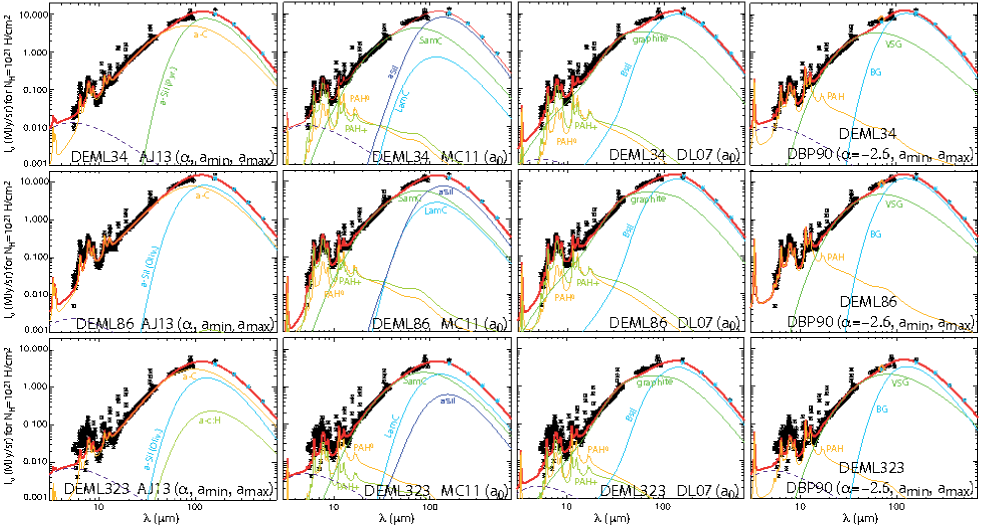
Figure 2: Continued

6.3 Changing the Radiation Field

Dust in galaxies can be illuminated by radiation field coming from different stellar populations. The Solar neighborhood RF is the standard RF used in most of modeling of dust emission. In order to see a possible improvement of our best modeling, as well as to test the robustness of our results, we also performed the modeling using other radiation fields. Bica et al. (1996) made a catalog of 504 star clusters and 120 stellar associations in the LMC using UBV photometry. They studied groups of stellar clusters with ages from 10 Myr to 16 Gyr. Kawamura et al. (2009) estimated that the youngest stellar objects are less than 10 Myr. Using the GALEV code we generated UV/visible spectrum of stellar clusters with various ages: 4-Myr, 60-Myr and 600-Myr. We then make the format of the output files compatible with the DustEM package (see Fig. 3). Results of the modeling using the 4-Myr RF are given in Tables 6.3, 6.3, LABEL:table_chi2_DL07 and LABEL:table_chi2_DBP90. Results of the fits using the 60-Myr and 600-Myr RFs and the corresponding figures are given in the appendix. We can see that changing the RF in the modeling has a direct impact on the values of dust abundances, and on the intensity of the RF in particular (see the following sections), but has a very limited impact on the reduced $\chi^{2}$. Therefore changing the RF does not improve the modeling, nor make it worse.

In addition, the impact of the RFs on the VSG dust size parameters is presented in Fig. LABEL:fig_alpha. The values of $a_{0}$ or $a_{min}$, $a_{max}$ can have some little variations but stay globally stable for MC11, DL07 and DBP90. For AJ13, the impact on $a_{min}$ is negligible, whereas $a_{max}$ is significantly affected for SSDR1, SSDR7 and SSDR9. This means that the $a_{max}$ values are not well constrained. The value of $\alpha$ do not vary much with the RF, except for SSDR9. However, the modeling of SSDR9 is of bad quality, whetever the RF. Therefore the analyis of this region using AJ13 should be considered very cautiously.

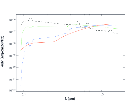
Figure 3: Radiation field templates used for the SED modeling: Mathis (solid red line), 4-Myr (short dashed black line), 60-Myr (dotted green line) and 600-Myr (long dashed blue line) stellar clusters.

Table 3: Best fit parameters for the ten regions obtained with AJ13, using the Mathis RF (top table) and 4-Myr RF (bottom table).

Table 4: Best fit parameters for the ten regions obtained with MC11, using the Mathis RF (top table) and 4-Myr RF (bottom table).

By changing the VSG dust size distribution ($\alpha$, $a_{min}$ and $a_{max}$), we can see that the excess does not appear anymore (see Fig. 2). This study reinforces the idea that in the framework of DBP90, the VSG size distribution in some regions of the LMC is different than that in our Galaxy. The analysis of the dust size distribution for all models is further discussed in the following Section 7.2.

It is known that the dust emission spectrum of the LMC shows a flattening in the submm compared to that of our Galaxy, which is even more pronounced in the SMC. At the same time, the SMC also shows a much larger excess of emission at 70 $\,{\rm\mu m}$ than the LMC (Bernard et al., 2008; Bot et al., 2010). We can therefore examine wether there is a possible link between the 70 $\,{\rm\mu m}$ excess and the submm flattening. For instance, in the LMC, this 70 $\,{\rm\mu m}$ excess and the submm flattening tend to disappear in most of the molecular gas phase, (Paradis et al., 2019). Note that this is not necessarily the case in molecular regions that may mix HI and CO gas phases. However, changing the VSG size distribution does not seem to have an impact on the submm flattening as the diffuse and HII regions have a distinct size distribution while exhibiting submm flattening (Paradis et al., 2019) (see Section 7.2). In the same way, the increase in the VSG relative abundance in the ionized gas of the LMC highlighted by Paradis et al. (2019) could explain the submm flattening observed in the ionized regions, but not in the atomic ones. In conclusion, a change in the size distribution or the relative abundance of VSGs or a combination of both could explain the difference in the submm emission observed in the LMC compared to our Galaxy. Therefore one could expect that the adequate change in the VSG size distribution and abundance in the SMC could help reproducing the 70 $\,{\rm\mu m}$ excess identified in Bot et al. (2004), and could result in a large contribution of the VSG emission in the submm-mm.

If dust mainly originates from carbon stars (Boyer et al., 2012), the large amount of carbon dust relative to the silicate dust could explain the emissivity behavior observed in the LMC. In other words, small carbon grains (or a combination of small and big carbon grains) could be responsible for the general behavior of the submm-mm flattening in the emission spectrum. For the SMC, the flattening seems to be too pronounced to be explained by carbon grains only. Indeed, in a previous study (unpublished) we found a submm emissivity spectral index of 0.9 in the SMC using IRIS (new processing of IRAS data Miville-Deschênes and Lagache, 2005) and Planck data. In addition, variations of the submm flattening have been observed in the diffuse medium of our Galaxy whereas the amount of VSG does not have any impact on the Galactic submm emission due to its low contribution at long wavelengths. The negligible submm emission from VSGs in our Galaxy, which shows a submm excess, indicates that the VSG component alone cannot be responsible of the submm excess observed in our Galaxy. Therefore, other processes might be at play, such as TLS (Two-Level-System) processes proposed by Mény et al. (2007), describing the amorphous state of large dust grains to explain the submm behavior observed in our Galaxy. The TLS model is able to reproduce the different dust emission behavior observed in our Galaxy (Paradis et al, 2011b; Paradis et al., 2012; Planck Collaboration XIV, 2014) and in the Magellanic Clouds (Planck Collaboration XVII, 2014). More recently, the TLS model was also fully able to reproduce observations in molecular complexes of our Galaxy such as the Perseus molecular cloud and W43 (Nashimoto et al., 2020)

To summarize, since in our Galaxy the VSG component emission is negligible in the submm range, the VSG contribution alone cannot be the origin of the submm excess. It is therefore most likely that the very pronounced and important submm flattening evidenced in the Magellanic Clouds originates from a combination of at least two emission processes: the emission from the VSG component plus the TLS processes in large grains; whereas only the TLS processes could be responsible for the local variations observed in the diffuse regions of the MW.

7.2 VSG size distribution: Diffuse versus HII regions

First, we compare the results obtained with the different models using the Mathis RF. For the same reason as in Section LABEL:sec_increase_vsg_mass, AJ13 is not discussed here since the a-C component includes both PAHs and small grains. We observe that the fits are significantly improved when changing some parameters of the VSG dust size distribution. The values of $a_{0}$ presented in Tables 6.3 and LABEL:table_chi2_DL07 show some variations from one model to the other. We observe values of $a_{0}$ going from 2 nm to 4.6 nm for MC11 and from 1 nm to 3.5 nm for DL07. Values for MC11 are close to the Galactic value of 2 nm in HII regions, whereas the values systematically increase in the diffuse regions. For DL07 all the values decrease compared to the Galactic ones. We observe the same trend for MC11: the values in HII regions are significantly lower than those in diffuse regions. Indeed, the mean value of $a_{0}$ in each type of environment is equal to 2.47 nm/1.34 nm in all HII regions with MC11/DL07, whereas the value is 4.17 nm/3.11 nm in diffuse regions with MC11/DL07. Molecular regions evidence intermediate values between these two extreme environments (diffuse and HII regions). We caution however that the mean value for each type of environment has been obtained with only two values for the diffuse and the molecular medium, and with six values for the ionized medium. This shift in the central value of the log-normal VSG size distribution in the different type of environments shows that HII regions contain mostly smaller VSGs (and less large grains in this component), and also an increase in the amount of small VSGs in comparison with the diffuse regions. For DBP90, the fits show lower values for both $a_{min}$ and $a_{max}$ (see Table LABEL:table_chi2_DBP90) in HII regions (mean values $a_{min}$=2.93 nm and $a_{max}$=13.1 nm) when compared to diffuse regions (mean values $a_{min}$=5.65 nm and $a_{max}$=20.3 nm), showing again smaller VSGs in HII regions than in the diffuse ones. The modeling with different RFs (Tables 8 to A) does not change these conclusions and confirms the trend observed with the use of the Mathis RF.

To summarize, our results indicate the same trend for all models, regardless the RF : the size distribution of VSGs is different in HII and diffuse regions with an increase in the quantity of small VSGs (and fewer large VSGs) in HII regions when compared to diffuse LMC regions. In this analysis, the SEDs represent the mixture of all gas phases (except for SSDR7 and SSDR9 that are almost pure atomic regions). For instance, SSDR1 and SSDR5 have a high level of HI emission, and most of the ionized regions of our sample have large column densities in the ionized gas as well as in other gas phases. We therefore expect a larger dispersion in the VSG size parameters, i. e. even more pronounced results, when analyzing dust emission associated with each gas phase independently. For instance, in SSDR8, DEML10 and DEML323 regions, the amount of Hydrogen column density in the HI gas phase is higher than in the H$\alpha$ gas phase. We therefore expect lower values of amin/amax or a0 (depending on the model) in these three regions, when looking at the H$\alpha$ gas phase only.

7.3 VSG lifecycle

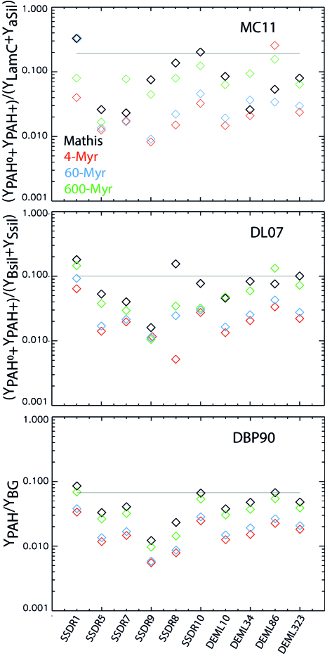
Figure 6: Ratio of the PAHs to the big grain component abundance, for the different models and for the ten regions, using different RFs (Mathis in black, 4-Myr in red, 60-Myr in blue and 600-Myr in green). The Galactic value is indicated with the gray line.

The results of this analysis show a significant increase in the VSG relative abundance compared to the MW. They also show an increase in smaller VSGs, compared to larger ones, in HII regions compared to the atomic medium. Some scenarios emphasize that, while Galactic dust could mainly be produced by O-rich AGB stars (67$\%$ and 20$\%$ from O-rich and C-rich AGBs, Gehrz, 1989), most of the dust in the Magellanic Clouds could originate from carbon stars (extreme AGB, i. e. mostly embedded carbon stars) with a dust production reaching 61$\%$ and 66$\%$ in the LMC and SMC (Boyer et al., 2012). The dust produced in such environments could consist in small carbon grains. Additional sources of dust production are supernovae, although their dust-destruction rates remain poorly constrained, and dust growth in the ISM. Another explanation to the enhancement of small carbon grains could be the destruction of large grains into smaller grains.

Regarding the enhancement of small VSGs in HII regions, two options could explain this behavior. First, (small) VSGs could be formed in HII regions rather than in molecular clouds, as proposed by Paradis et al. (2019). Indeed, in their study they have shown that the relative abundance of VSGs is enhanced in the ionized phase of the gas, whatever the nature of the clouds, ie quiescent or forming stars, and independently of the intensity of the radiation field. Such VSGs could be large PAH clusters or cationic PAH clusters (Rapacioli et al., 2005, 2011; Roser and Ricca, 2020). Then, whatever the nature of these grain species, grain growth could occur in the atomic and molecular regions, via accretion or coagulation, and could explain the presence of larger VSGs in the molecular and diffuse environments. To examine the hypothesis that PAH clusters could be responsible of the VSG increase in the LMC, we present in Fig. 6 the PAH relative abundance for each model (except AJ13) and region. First, for all models, the PAH relative abundance is lower than the Galactic value in agreement with the hypothesis of the presence of PAH clusters. However, Fig. 6 does not show any trend with the nature of the region, unlike in the case of the VSGs. This absence of real trend suggests that other processes might occur. For instance, the BG component could be also affected by strong shocks and turbulence, and contribute to increase the relative abundance of VSGs, as observed in the LMC. In this second option, the largest VSGs could be destroyed in HII regions in shocks, resulting in an increase of the amount of smallest VSGs. This effect could be the result of supernova explosions or turbulence. This hypothesis could explain the changes in size of the VSG population. As these two processes most likely both occur, the VSG component could include two distinct populations: small VSGs originating from large PAH clusters or cationic PAHs clusters, mainly formed in HII regions, and large VSGs resulting from BG destruction.

Heiles et al. (2000) analyzed the Barnard’s Loop HII region and evidenced an increase of the 60 $\,{\rm\mu m}$ emission. They showed that this increase is not the consequence of the presence of warm big grains and proposed that it could be due to an enhancement of the VSG population relative to BGs in the ionized region compared to the global neutral medium. As a consequence it appears that the increase in the VSG relative abundance in the ionized medium could be a more general result than just an isolated result concerning the LMC. Jones et al. (1996) have developed an analytical model to derive the fragment size distribution as well as the final crater mass in grain-grain collisions depending on different parameters (grain properties, sizes and collision velocity). They found that grain shattering leads to the redistribution of the dust mass from large grains into smaller grains. More recently, Hirashita (2010) has theoretically studied interstellar shattering of large grains (a$\sim$0.1 $\,{\rm\mu m}$) to explain the production of small grains. They were able to reproduce the small grain abundance derived by Mathis et al. (1983) in the warm neutral medium. They also showed that additional shattering in the warm ionized medium could destroy carbonaceous grains with a size of $\sim$0.01 $\,{\rm\mu m}$ and generate smaller grains. On the opposite silicate grains are harder to shatter than graphite. However, in this study (see Table LABEL:table_chi2_DL07), we observe in four regions high abundances of small silicates compared to large silicates with DL07. According to the theory of Hirashita (2010), we cannot explain this enhancement of small silicates as resulting from large silicate destruction nor from another source of production.

A recent analysis of the turbulence in the LMC (Szotkowski et al., 2019) evidenced spatial variations of HI turbulent properties. The turbulence is often characterized by estimating spatial power spectrum (SPS) of intensity fluctuations. The authors pointed out several localized steepening of the small-scale SPS slope around HII regions, and around 30 Doradus in particular, in agreement with numerical simulations (Grisdale et al., 2017, 2019) suggesting steepening of the SPS slope due to stellar feedback eroding and destroying small clouds. This study is in agreement with the possible additional grain shattering in the ionized medium, i. e. in HII regions, where we observe the smallest VSG populations when compared to the atomic and molecular environments.

7.4 Extinction

For the four tested models, it is always possible to find a set of parameters that correctly fits the emission part of the SED. Fitting the dust emission from NIR to FIR wavelength therefore does not allow us to unambiguously determine which dust models best reproduce the observations. In the context it is interesting to check wether these best-fit models also show similar extinction curves or whether extinction data could help to differentiate between the different grain models.

Comparing the modeled extinction curves with observations is not easy because we do not have extinction curves associated to the studied regions. In the Milky Way, a wide variety of possible shapes of these curves has been observed (Papaj et al., 1991; Megier et al., 1997; Barbaro et al., 2001; Wegner, 2002; Fitzpatrick and Massa, 2007; Gordon et al., 2021) and we can similarily expect the extinction curves in the LMC have different profiles. This was observed by Gordon et al. (2003) who found that the LMC averaged extinction curve is characterized by a stronger far-UV rise than the one of the MW, and by a weaker 2175 Å bump (see for instance LMC2-supershell, near the 30 Doradus starbursting region). The authors argue that the difference between the extinction curves of the Magellanic Clouds and the MW could be due to the fact that the observed environments are different. For the Magellanic Clouds, the extinction curves are observed in active star formation regions where large grains could be destroyed by strong shocks and/or UV photons. Nevertheless, the sample of LMC extinction curves is quite limited compared to that of our Galaxy.

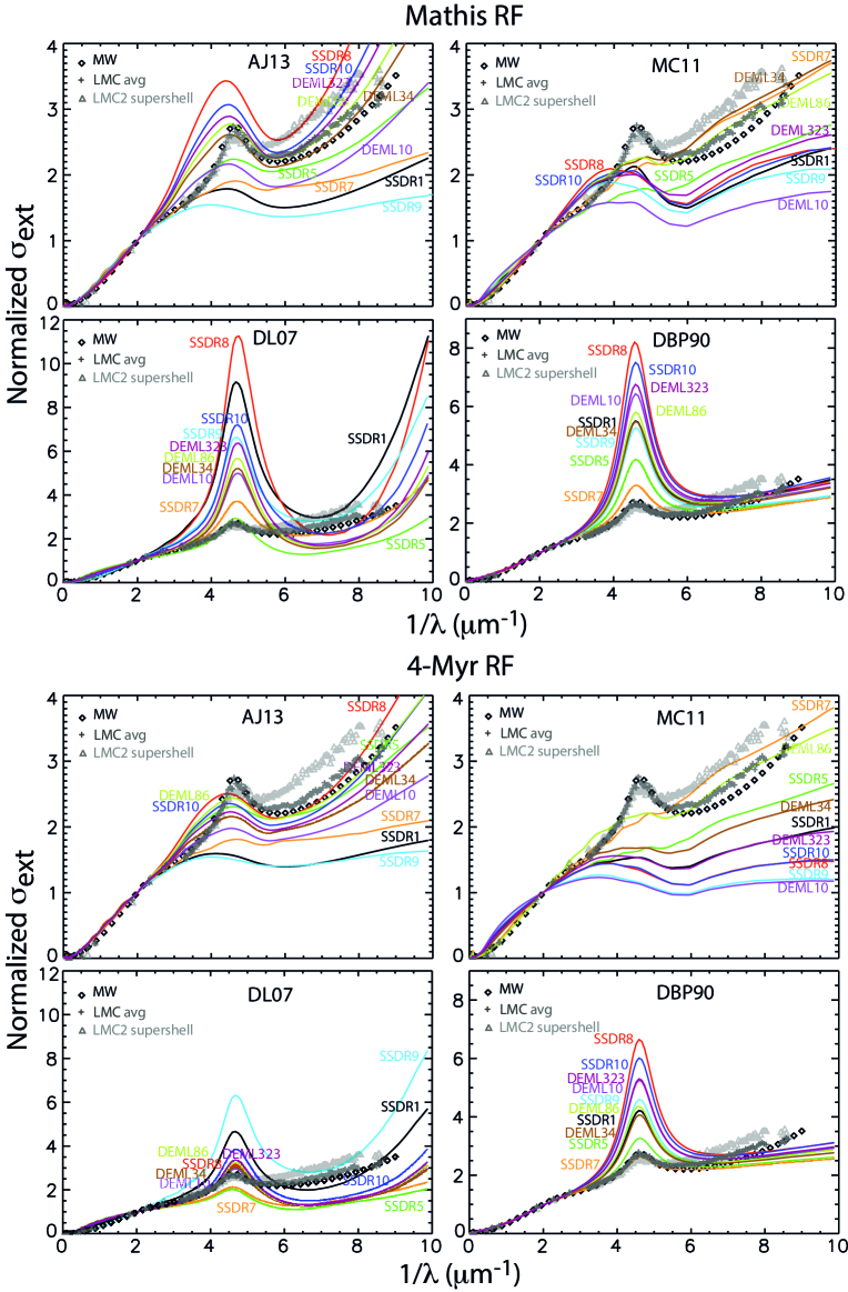
Figure 7: Extinction curves for each region, derived from the different dust models, with Mathis RF (top) and 4-Myr RF (bottom). The averaged Galactic and LMC extinction curves are given in black diamonds and dark gray crosses for comparison. The LMC2 supershell extinction curve is presented with light gray triangles. Caution: the scales have been chosen to show the difference between the different models in a clear way, and one should take this into account in the comparisons.

The extinction curves calculated by DustEM for the different dust best-fit models are shown in Figs. 7 and 11 as well as, for comparison, the average LMC and LMC2-supershell extinction curves (Gordon et al., 2003) and the average Galactic extinction curve representative of the interstellar medium (Cardelli et al., 1989). We notice that the predicted extinction curves are highly model dependent, are also different from one region to another and are sensitive to the RF. According to the model predictions computed using the Mathis RF (Fig. 7) the extinction curves of DL07 and DBP09 models show a prominent 2175 $\AA$ bump followed by a fast far-UV rise in the case of DL07 for all regions. Such strong bumps are not observed in our Galaxy or in the Magellanic Clouds. On the other hand, the extinction curves of all regions modeled with MC11 have large and flattened bumps (except for SSDR7 that does not show any bump at all). When the DBP90 model is used we notice a significant increase in the bump from diffuse/molecular to HII regions. The extinction curves calculated with the AJ13 model show different behaviors depending on the region, with a weaker 2175 $\AA$ bump in diffuse/molecular regions than in ionized regions. The UV bumps are significantly stronger in the extinction curves calculated with DL07 and DBP90 than with AJ13 which are the closest to the observed extinction curves.

Changing the RF has a strong effect on the extinction curves, and more specifically on the 2175 $\AA$ bump whose strength decreases when the strength of the RF increases (see Figs. 7 and 11). However, for some regions and models the bump remains unchanged, e.g. for SSDR9 and DL07. The extinction curves calculated with the 4-Myr RF are in better agreement with the Galactic and LMC behaviors, in contrast with those calculated using Mathis RF and 60-600 Myr RFs. In models using the 4-Myr RF, the extinction curves calculated for DL07 and DBP90 models evidence the strongest 2175 $\AA$ bumps, whereas MC10 shows very flat bumps and UV-rise for almost all the regions. AJ13 model seems to minimize the discrepancies between predictions and observations, which makes this model more compatible with LMC curves than the other models.

Even if it is hard to interpret such results since we do not have the extinction curve associated to the different studied regions, no model seems to give a satisfactory prediction. However, we now know that the dust emission models give very distinct behaviors in terms of extinction predictions. This point is important and should be used to refine constraints on the dust models themselves. For instance, maybe if models consider a two-population of VSG component, as discussed in Section 7.3, with only one carbonaceous component such as large PAH clusters or cationic PAHs impacting the 2175 $\AA$ bump, maybe they would better reconcile with extinction curves. Moreover, it appears that the extinction curves can also play an important role to better constrain the RF of each environments. These preliminary results, in terms of extinction description, seem to indicate that the Mathis RF is not the best to be used in the Magellanic Clouds, and suggest that maybe stronger RFs are necessary.

Recently, new cosmic dust models have been or will soon be made available (Hensley and Draine, 2022; Siebenmorgen, 2022; Ysard, 2020). It would be interesting to continue this study by using these models to fit the LMC observations, both in emission and extinction. Finally, this work highlights the fact that future studies should, if possible, simultaneously fit dust emission and extinction.

8 Conclusion

Using Spitzer IRS, MIPS SED and photometric data combined with Herschel data, we performed modeling of the spectra in diffuse, molecular and HII regions of the LMC. We compared four distinct dust models available in the DustEM package: Jones et al. (2013) (AJ13), Compiègne et al. (2011) (MC11), Draine and Li (2007) (DL07) and an updated version of Désert et al. (1990) (DBP90). To check the robustness of the results, we adopted four different radiation fields (interstellar RF or Mathis, stellar clusters with various ages: 4-Myr, 60-Myr and 600-Myr). None of the models is able to reproduce the MIR-to-FIR emission using the Galactic standard parameters even when the abundances of the dust components and the radiation field strength are allowed to vary. Changes in the size distribution and abundances of the dust component that dominates the MIR-to-FIR emission (commonly referred to as very small grains or VSGs) are needed to reasonably fit the dust emission spectra.

One of the first results of this analysis is the significant increase of the VSG abundance relative to the big grain (BG) component in the LMC compared to the Milky-Way. Changes in the size distribution and abundance of dust have a clear impact on the contribution of the VSG emission in the submm. Depending on the model, the VSG component can strongly dominate the submm emission, especially when using the standard Mathis RF. Although no correlation could be shown between this strong VSG emission in the submm and the type of environment, care should be taken when analysing the FIR to submm emission in the LMC using only the big grain component. Small carbon grains could be partly responsible for the global submm-mm flattening observed in the LMC, even if other processes might be at play to explain local variations observed in the LMC and the Milky-Way. The 70 $\,{\rm\mu m}$ emission excess evidenced in previous studies of the Magellanic Clouds could result from distinct VSG properties (size distribution and abundances) compared to our Galaxy.

Another important result is an increase in the amount of small VSGs (and a decrease of big VSGs) in HII regions when compared to diffuse regions of the LMC. In contrast to our Galaxy, where dust could mainly be produced by O-rich AGB stars, some dust in the LMC could come from C-rich AGB stars (extreme AGB, i. e. mosty embedded carbon stars). The presence of small VSGs in HII regions could be explained by: - the formation of small VSGs in HII regions (rather than in molecular clouds); grain growth could occur in the diffuse and molecular medium via accretion or coagulation processes. - the destruction of the largest VSGs and BG component in HII regions by shocks resulting from supernova explosions or turbulence. If these two scenarios take place, the VSG component could include two populations : small VSGs resulting from large PAH clusters or cationic PAH clusters, and large VSGs resulting from BG destruction.

The extinction curves calculated by DustEM show a great diversity of behaviors according to dust models and radiation fields. The AJ13 model shows reasonable predictions when compared to the ”usual” behaviors. In the LMC stronger RFs seem to reproduce the shape of the extinction curve better, in particular by reducing the strong 2175 Åbump predicted by the models. Observations in the LMC are in that sense important to better constrain the dust models (and more specifically the VSG component) but also to better constrain the RFs. Further studies simultaneously fitting dust emission and extinction and/or using the latest grain models should provide better constraints on the properties of grains in the LMC and other galaxies.

Appendix A Additional material

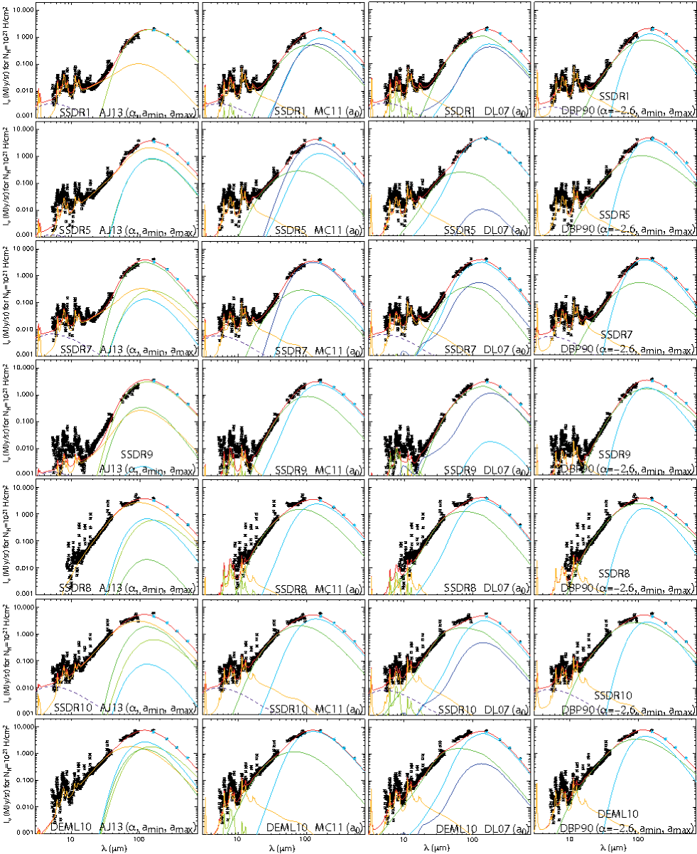
Figure 8: Modeling of the SEDs of the ten regions with different dust models and free parameters ($\rm X_{ISRF}$, dust abundances and small grains dust size distribution), using the 4-Myr RF. The observations (Spitzer IRS SS and LL, MIPS SED, MIPS 160 $\,{\rm\mu m}$, Herschel Photometric PACS 160 $\,{\rm\mu m}$ and SPIRE 250 $\,{\rm\mu m}$, 350 $\,{\rm\mu m}$ and 500 $\,{\rm\mu m}$ data) are shown in black. The total modeled SED is shown as a red line. The other colored lines correspond to the different dust components of the models (see Fig. 1 or 2). The dashed line represents the additional NIR continuum. Blue asterisks show the color-corrected brightness derived from the models. Each column shows the fit using different dust models (from left to right: AJ13, MC11, DL07 and DBP90). Each row presents a different region. The figure continues on the next page.

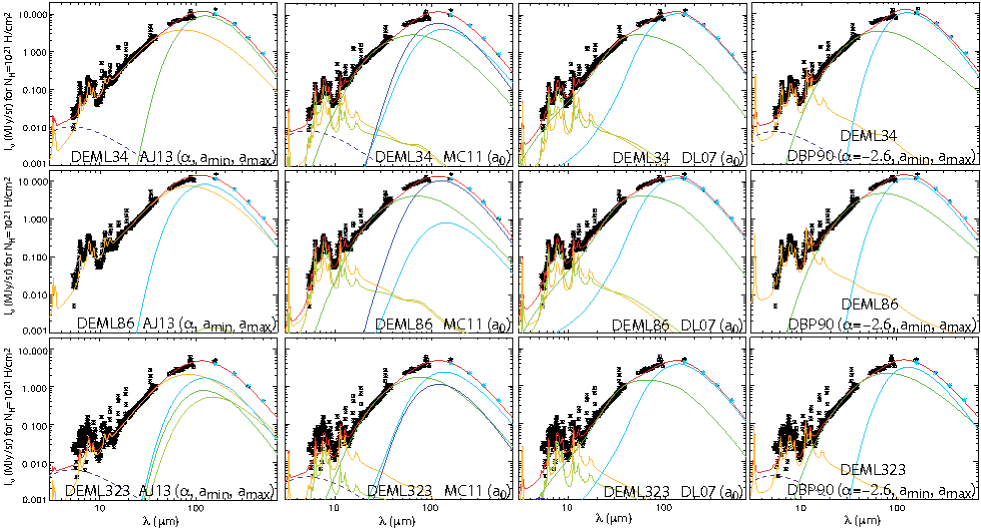
Figure 8: Continued

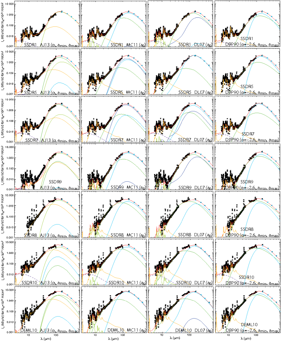
Figure 9: Modeling of the SEDs of the ten regions with different dust models and free parameters ($\rm X_{ISRF}$, dust abundances and small grains dust size distribution), using the 60-Myr RF. The observations (Spitzer IRS SS and LL, MIPS SED, MIPS 160 $\,{\rm\mu m}$, Herschel Photometric PACS 160 $\,{\rm\mu m}$ and SPIRE 250 $\,{\rm\mu m}$, 350 $\,{\rm\mu m}$ and 500 $\,{\rm\mu m}$ data) are shown in black. The total modeled SED is shown as a red line. The other colored lines correspond to the different dust components of the models (see Fig. 1 or 2). The dashed line represents the additional NIR continuum. Blue asterisks show the color-corrected brightness derived from the models. Each column shows the fit using different dust models (from left to right: AJ13, MC11, DL07 and DBP90). Each row presents a different region. The figure continues on the next page.

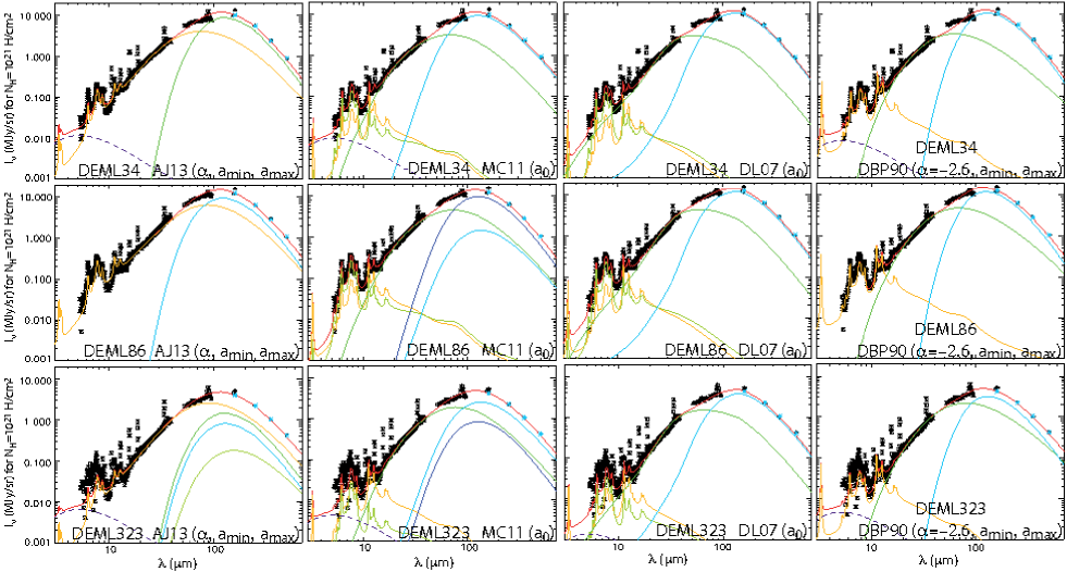
Figure 9: Continued

Figure 10: Modeling of the SEDs of the ten regions with different dust models and free parameters ($\rm X_{ISRF}$, dust abundances and small grains dust size distribution), using the 600-Myr RF. The observations (Spitzer IRS SS and LL, MIPS SED, MIPS 160 $\,{\rm\mu m}$, Herschel Photometric PACS 160 $\,{\rm\mu m}$ and SPIRE 250 $\,{\rm\mu m}$, 350 $\,{\rm\mu m}$ and 500 $\,{\rm\mu m}$ data) are shown in black. The total modeled SED is shown as a red line. The other colored lines correspond to the different dust components of the models (see Fig. 1 or 2). The dashed line represents the additional NIR continuum. Blue asterisks show the color-corrected brightness derived from the models. The orange diamonds that are visible in the DBP90 panels show the MIPS 70 $\,{\rm\mu m}$ photometric data normalized to the integrated flux in the MIPS-SED band. Each column shows the fit using different dust models (from left to right: AJ13, MC11, DL07 and DBP90). Each row presents a different region. The figure continues on the next page.

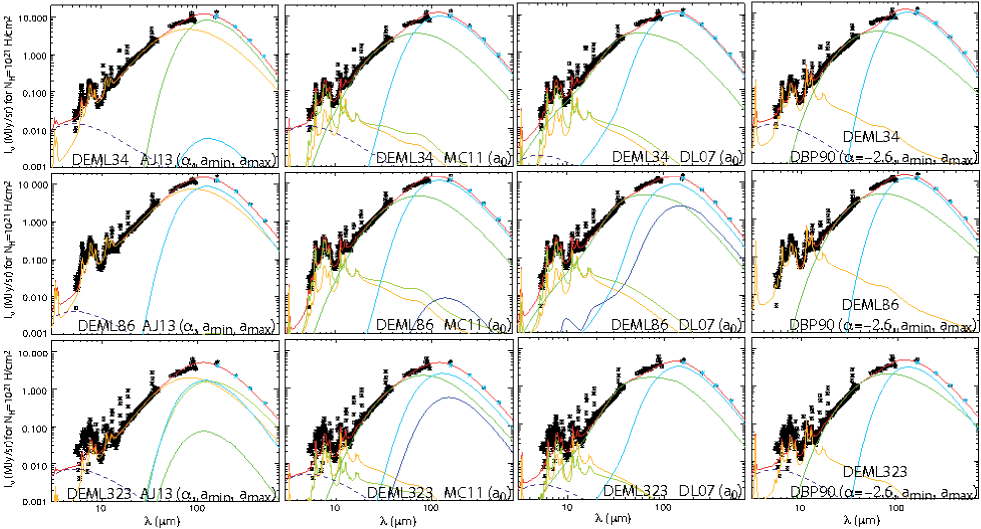
Figure 10: Continued

Table 8: Same table as Table 6.3 but using a 60-Myr (top) and 600-Myr RF (bottom).

AJ13 ($\alpha,a_{min},a_{max}$) - 60-Myr RF
Region	$\chi^{2}/dof$	$X_{ISRF}$	$Y_{a-C}$	$Y_{a-C:H}$	$Y_{Pyr.}$	$Y_{Oliv.}$	$Y_{dust,tot}$	$I_{NIR\,cont.}$	$\alpha$	$a_{min}$	$a_{max}$	$\frac{Y_{a-C}}{Y_{Sil.}+Y_{a-C:H}}$
							($10^{-2}$)	($10^{-3}$)		($10^{-1}$)		($10^{-1}$)
SSDR1	2.42	0.59	1.08$\times 10^{-4}$	1.71$\times 10^{-3}$	1.00$\times 10^{-6}$	1.00$\times 10^{-6}$	0.18	3.59	-4.34	4.00	13.3	0.631
SSDR5	6.01	0.25	4.83$\times 10^{-4}$	1.96$\times 10^{-3}$	9.70$\times 10^{-3}$	4.15$\times 10^{-5}$	1.22	1.16	-3.07	4.00	5.57	0.413
SSDR7	3.53	0.47	2.36$\times 10^{-4}$	4.07$\times 10^{-4}$	6.26$\times 10^{-3}$	1.00$\times 10^{-6}$	0.69	7.00	-4.03	4.00	11.7	0.354
SSDR9	10.6	0.58	1.71$\times 10^{-4}$	2.30$\times 10^{-3}$	6.97$\times 10^{-4}$	2.53$\times 10^{-6}$	0.32	1.33	-3.31	4.18	3830	0.570
SSDR8	3.71	0.97	4.28$\times 10^{-4}$	1.66$\times 10^{-3}$	1.00$\times 10^{-6}$	1.70$\times 10^{-5}$	0.21	0.00	-2.00	14.7	6.25	2.55
SSDR10	2.71	0.86	8.31$\times 10^{-4}$	2.18$\times 10^{-3}$	7.19$\times 10^{-5}$	4.96$\times 10^{-4}$	0.36	11.2	-2.44	4.00	6.64	3.02
DEML10	4.34	0.67	9.30$\times 10^{-4}$	2.54$\times 10^{-3}$	4.23$\times 10^{-3}$	4.68$\times 10^{-5}$	0.77	0.558	-2.12	5.93	5.00	1.36
DEML34	1.56	0.30	5.80$\times 10^{-3}$	1.00$\times 10^{-6}$	2.32$\times 10^{-2}$	1.00$\times 10^{-6}$	2.90	11.6	-2.09	4.00	5.09	2.50
DEML86	2.18	0.40	5.87$\times 10^{-3}$	1.00$\times 10^{-6}$	1.00$\times 10^{-6}$	1.99$\times 10^{-2}$	2.58	0.00	-2.70	4.00	6.90	2.95
DEML323	3.80	0.29	2.89$\times 10^{-3}$	2.79$\times 10^{-4}$	4.05$\times 10^{-3}$	2.28$\times 10^{-3}$	0.95	6.45	-2.00	4.00	6.47	4.37
AJ13 ($\alpha,a_{min},a_{max}$) - 600-Myr RF
Region	$\chi^{2}/dof$	$X_{ISRF}$	$Y_{a-C}$	$Y_{a-C:H}$	$Y_{Oliv}$	$Y_{Pyr.}$	$Y_{dust,tot}$	$I_{NIR\,cont.}$	$\alpha$	$a_{min}$	$a_{max}$	$\frac{Y_{a-C}}{Y_{Sil.}+Y_{a-C:H}}$
							($10^{-2}$)	($10^{-3}$)		($10^{-1}$)		($10^{-1}$)
SSDR1	2.44	3.17	1.96$\times 10^{-4}$	1.59$\times 10^{-3}$	4.25$\times 10^{-6}$	6.42$\times 10^{-6}$	0.18	4.18	-4.45	4.00	13.3	1.22
SSDR5	5.72	1.13	2.17$\times 10^{-3}$	6.32$\times 10^{-4}$	4.75$\times 10^{-3}$	6.35$\times 10^{-3}$	1.39	1.63	-3.12	4.00	10.4	1.85
SSDR7	3.57	3.31	4.35$\times 10^{-4}$	4.00$\times 10^{-4}$	4.73$\times 10^{-3}$	1.00$\times 10^{-6}$	0.56	7.88	-4.10	4.00	180	0.848
SSDR9	11.2	4.03	5.42$\times 10^{-5}$	2.26$\times 10^{-3}$	6.27$\times 10^{-6}$	1.00$\times 10^{-6}$	0.23	0.439	-4.37	4.68	4680	0.239
SSDR8	3.65	1.26	5.43$\times 10^{-3}$	1.00$\times 10^{-6}$	1.00$\times 10^{-6}$	1.35$\times 10^{-3}$	0.68	0.00	-2.00	13.7	6.70	40.2
SSDR10	3.01	7.28	5.10$\times 10^{-4}$	2.14$\times 10^{-3}$	1.00$\times 10^{-6}$	1.00$\times 10^{-6}$	0.27	13.7	-2.29	4.00	3.84	2.38
DEML10	4.25	5.04	1.11$\times 10^{-3}$	2.52$\times 10^{-3}$	1.81$\times 10^{-3}$	2.16$\times 10^{-4}$	0.57	1.63	-2.15	6.16	4.26	2.44
DEML34	1.57	1.89	8.88$\times 10^{-3}$	1.00$\times 10^{-6}$	2.00$\times 10^{-2}$	1.50$\times 10^{-5}$	2.89	14.5	-2.04	4.00	4.43	4.44
DEML86	2.26	2.70	8.29$\times 10^{-3}$	1.00$\times 10^{-6}$	1.00$\times 10^{-6}$	1.63$\times 10^{-2}$	2.46	4.12	-2.69	4.00	5.95	5.09
DEML323	3.79	3.74	1.61$\times 10^{-3}$	1.10$\times 10^{-3}$	1.04$\times 10^{-4}$	2.41$\times 10^{-3}$	0.52	7.35	-2.00	4.00	5.08	4.45

Table 9: Same table as Table 6.3 but using a 60-Myr (top) and 600-Myr RF (bottom).

Table 10: Same table as Table LABEL:table_chi2_DL07 but using a 60-Myr (top) and 600-Myr RF (bottom).

Table 11: Same table as Table LABEL:table_chi2_DBP90 but using a 60-Myr (top) and 600-Myr RF (bottom).

Table 12: Ratio of the small grain component emission to the total dust emission for each best-fit model using the 60-Myr (top table) and 600-Myr RF (bottom table), at 250, 500, 850 and 1100 $\,{\rm\mu m}$.

		60-Myr RF
	AJ13				MC11				DL07				DBP90
Best modeling	($\alpha$, $a_{min}$, $a_{max}$)				($a_{0}$)				($a_{0}$)				($\alpha=-2.6$, $a_{min}$, $a_{max}$)
	$I^{a-C}_{\nu}/I^{tot}_{\nu}$ ($\%$)				$I^{SamC}_{\nu}/I^{tot}_{\nu}$ ($\%$)				$I^{graph.}_{\nu}/I^{tot}_{\nu}$ ($\%$)				$I^{VSG}_{\nu}/I^{tot}_{\nu}$ ($\%$)
Wavelengths	250	500	850	1100	250	500	850	1100	250	500	850	1100	250	500	850	1100
SSDR1	1.6	1.2	1.0	1.0	10.3	8.7	8.7	8.8	69.2	53.3	44.7	41.3	20.0	27.1	39.7	47.1
SSDR5	1.9	1.9	2.1	2.2	2.9	2.4	2.7	2.9	1.2	1.0	1.1	1.1	9.2	12.1	19.0	23.9
SSDR7	2.8	3.4	4.1	4.5	7.5	6.6	7.5	8.2	5.2	4.4	4.1	4.0	5.5	8.7	14.6	18.8
SSDR9	7.1	6.0	5.5	5.4	8.1	7.0	7.0	7.0	59.1	44.0	36.0	33.0	21.8	29.1	42.0	49.4
SSDR8	12.0	9.4	8.6	8.4	17.1	15.1	15.7	16.0	28.6	22.6	22.9	23.5	35.8	46.1	60.2	67.1
SSDR10	14.6	11.9	11.0	10.7	14.2	12.8	13.3	13.7	6.4	5.5	5.9	6.1	22.0	26.8	38.0	45.0
DEML10	6.4	5.7	5.7	5.7	4.2	3.9	4.2	4.4	4.2	3.6	3.9	4.1	21.0	27.8	40.0	47.3
DEML34	15.3	19.2	25.5	29.3	6.7	6.4	6.9	7.2	3.7	3.4	3.8	4.0	5.1	5.9	9.1	11.6
DEML86	26.1	31.1	38.9	43.2	16.0	14.5	17.0	18.6	5.9	5.3	5.7	6.0	8.1	10.1	15.6	19.7
DEML323	34.0	38.3	44.7	47.9	13.9	12.7	13. 6	14.0	6.8	5.9	6.4	6.7	15.4	18.9	27.9	33.9
		600-Myr RF
SSDR1	2.7	2.1	1.9	1.9	37.4	34.9	36.6	37.8	72.5	64.8	58.3	55.2	31.9	46.6	61.6	68.4
SSDR5	23.9	28.0	32.4	34.7	4.9	3.9	5.4	5.7	3.0	2.9	3.0	3.1	17.8	28.2	41.8	49.2
SSDR7	10.8	13.1	15.3	16.3	7.3	7.0	7.0	7.0	15.7	14.0	12.3	11.6	11.3	19.9	31.3	37.9
SSDR9	0.9	0.7	0.7	0.7	34.9	32.6	32.5	32.5	45.5	38.3	32.4	29.7	34.8	50.1	64.9	71.4
SSDR8	87.4	90.3	92.8	93.4	37.5	36.3	37.2	37.7	33.2	31.1	31.7	32.2	53.6	69.1	80.4	84.7
SSDR10	4.6	3.5	3.1	2.9	29.5	28.8	29.6	30.0	24.4	23.0	23.9	24.4	36.8	50.2	64.5	71.0
DEML10	8.5	7.3	6.8	6.6	10.1	10.2	10.7	11.0	11.3	10.9	11.5	11.9	36.3	51.7	66.1	72.4
DEML34	25.4	31.8	39.1	43.1	12.3	12.6	13.4	13. 7	8.8	8.9	9.7	10.0	10.6	15.8	24.6	30.
DEML86	38.3	45.6	53.6	57.7	14.3	14.5	15.1	15.3	13.2	12.8	12.8	12.7	15.7	23.7	35.5	42.5
DEML323	24.6	23.8	23.9	23.9	24.3	24.3	25.7	26.3	17.5	16.9	17.7	18.1	27.9	39.7	54.2	61.4

Figure 11: Extinction curves for each region, derived from the different dust models, with 60-Myr RF (left) and 600-Myr (right). The averaged Galactic and LMC extinction curves are given in black diamonds and dark gray crosses for comparison. The LMC2 supershell extinction curve is presented with light gray triangles. Caution: the scales have been chosen to show the difference between the different models in a clear way, and one should take this into account in the comparisons.