Weak Convergence of Tamed Exponential Integrators for Stochastic Differential Equations

Abstract.

We prove weak convergence of order one for a class of exponential based integrators for SDEs with non-globally Lipschtiz drift. Our analysis covers tamed versions of Geometric Brownian Motion (GBM) based methods as well as the standard exponential schemes. The numerical performance of both the GBM and exponential tamed methods through four different multi-level Monte Carlo techniques are compared. We observe that for linear noise the standard exponential tamed method requires severe restrictions on the stepsize unlike the GBM tamed method.

1. Introduction

We consider weak convergence analysis of tamed schemes for semi-linear Stochastic Differential Equations (SDEs) of the form

(1) $$dX_{t}=\left(AX_{t}+F(X_{t})\right)dt+\sum_{i=1}^{m}\left(B_{i}X_{t}+g_{i}(X_{t})\right)dW_{t}^{i},\quad X_{0}=x\in\mathbb{R}^{d},$$

with $m$, $d\in\mathbb{N}$. Here $W_{t}^{i}$ are iid Brownian motions on the probability space $(\Omega,\mathcal{F},\mathbb{P})$ with filtration $({\mathcal{F}_{t}})_{t\in[0,T]}$. The nonlinearity $F:\mathbb{R}^{d}\rightarrow\mathbb{R}^{d}$ only satisfies a one sided Lipschitz condition, where as the $g_{i}:\mathbb{R}^{d}\rightarrow\mathbb{R}^{d}$ are globally Lipschitz (see Assumption 1). We assume throughout that the matrices $A$, $B_{i}\in\mathbb{R}^{d\times d}$ satisfy the following zero commutator conditions

(2) $$AB_{i}-B_{i}A=0,\quad B_{j}B_{i}-B_{i}B_{j}=0\qquad\text{for}\quad i,j=1,\ldots,m.$$

By introducing the shorthand notation

(3) $$\mu(y):=Ay+F(y),\quad\sigma_{i}(y):=B_{i}y+g_{i}(y),$$

and the matrix $\sigma(x)=[\sigma_{i}(x)]$, (i.e. columns formed by $\sigma_{i}$) we can re-write (1) as

$$dX_{t}=\mu(X_{t})dt+\sigma(X_{t})dW.$$

The schemes we examine are in the class of exponential integrators. These methods have proved to be effective schemes for many SDEs and stochastic partial differential equations (SPDEs). Originally only linear (or linearized) drift terms were exploited, see for example [21, 3, 24, 16, 15], however recently several exponential integrators that also exploit the linear terms in diffusion emerged [14, 9, 8, 29]. We are particularly interested in dealing with a one-sided Lipschitz drift term $F$ with superlinear growth. Hutzenthaler et al. [12] showed both strong and weak divergence Euler’s method for the general SDE (1) with superlinearly growing coefficients $F$ and/or $g_{i}$. Following [12] many explicit variants of Euler-Maruyama schemes that guarantee the strong convergence to the exact solution of SDE were derived, see for example [13, 23, 2, 19, 30, 27]. The most well known approach to deal with superlinearly growing coefficients is to employ ”taming” to prevent the unbounded growth of numerical solutions. Although there has been much consideration of strong convergence of tamed schemes, see for example [13, 25, 26] there has been little consideration of weak convergence for SDEs [5, 4, 28]. In [5], Bréhier investigated the weak error of the explicit tamed Euler scheme for SDE’s with one-sided Lipschitz continuous drift and additive noise to approximate averages with respect to the invariant distribution of the continuous time process. Bossy et al., [4], proposed and proved weak convergence of a semi-explicit exponential Euler scheme for a one-dimensional SDE with non-globally Lipschitz drift and diffusion behaving as $x^{\alpha}$, with $\alpha>1$. Due to the weak condition on the diffusion coefficient, their study covers regularity results for the solution of the Kolmogorov PDE commonly used in weak error analysis. In [28], Wang and Zhao formulated a general weak convergence theorem for one-step numerical approximations of SDEs with non-globally drift coefficients. They applied this to prove weak convergence of rate one for the tamed and backward Euler-Maruyama methods. We would like to point out that their analysis is not directly applicable to our GBM based schemes as it is not a classical one-step method but rather the composition of the GBM flow and a one-step flow. In the context of SPDEs, Cai et al. [6] constructed and analysed a weak convergence of a numerical scheme based on a spectral Galerkin method in space and a tamed version of the exponential Euler method. Below we impose conditions that are similar to those for the SPDE in [6].

We prove weak convergence for a class of exponential integrators where a form of taming is used for the one-sided Lipschitz drift term. The GBM methods exploit the exact solution of geometric Brownian motion, see [9] and [10] where strong convergence of related methods were considered. Further, by taking $A=B_{i}=0$ we simultaneously prove weak convergence for the standard exponential tamed scheme such as in [13]. Our proof is based on the Kolmogorov equation and one of the main difficulties is to take into account the stochasticity in the solution operator.

In our numerical experiments we compare different approaches to estimate the weak errors all using multi-level Monte Carlo (MLMC) techniques as reviewed in [11]. For a linear diffusion term we observe that the exponential tamed method does not perform well for larger timesteps and hence a timestep restriction is required for MLMC techniques (for example to estimate the weak errors). This is of particular interest as tamed methods were originally introduced and strong convergence was examined precisely to control nonlinearities in the context of MLMC type simulations, see [13]. The GBM based method does not suffer in this way in our experiments for linear noise. For nonlinear diffusion both tamed based methods require a step size restriction for convergence on the MLMC techniques.

The paper is organized as follows: in Section 2 we state our assumptions on the drift and diffusion, present the new numerical method and state our main results. In Section 3 we present numerical simulations illustrating the rate of convergence using the MLMC simulations and compare the different approaches. The proofs of the main results are then given in detail in Sections 4 and 5.

2. Setting and Main Results

Throughout the paper we let ${\big{\langle}}\cdot,\cdot{\big{\rangle}}$ denote the standard inner product in $\mathbb{R}^{d}$ (so ${\big{\langle}}y,z{\big{\rangle}}=y^{\intercal}z$ for $y,z\in\mathbb{R}^{d}$ ) and $\left\lVert\cdot\right\rVert$ represent both the Euclidean norm for vectors as well as the induced matrix norm. A vector $\beta=(\beta_{1},\beta_{2},\ldots,\beta_{d})$ is a multiindex of order $|\beta|=\sum_{i=1}^{d}\beta_{i}$ with nonnegative integers components. The partial derivative operator corresponding to the multiindex $\beta$ is defined as

$$D^{\beta}h(x)=\frac{\partial^{|\beta|}h(x)}{\partial_{x_{1}}^{\beta_{1}}\partial_{x_{2}}^{\beta_{2}}\ldots\partial_{x_{d}}^{\beta_{d}}}$$

where $h\in C^{|\beta|}(\mathbb{R}^{d};\mathbb{R}^{l})$. For a nonnegative integer $j$, we let $\mathbf{D}^{j}h(x)$ represent the jth order derivative operator applied to a function $h\in C^{j}(\mathbb{R}^{d};\mathbb{R}^{l})$. When $j=1$ we simply write the Jacobian as $\mathbf{D}h$. We define the sets

$$\mathbb{N}_{n}:=\{0,1,2,\ldots,n\}\qquad\text{and}\qquad\mathbb{N}_{n}^{+}:=\{1,2,\ldots,n\}.$$

Before presenting our class of numerical methods we state our assumptions on the drift $F$ and diffusion $g_{i}$ for the SDE (1).

Assumption 1.

Let $F,g_{i}\in C^{4}(\mathbb{R}^{d};\mathbb{R}^{d})$ for $i=1,2\ldots,m$ and let there exist $r\geq\rho$, $r\geq 0$ and $K,c,a,\gamma>0$, such that for all $y,z\in\mathbb{R}^{d}$ and $j=0,1,2,3,4$

1. $\sup_{y\in\mathbb{R}^{d}}\left\lVert D^{\alpha}F(y)\right\rVert(1+\left\lVert y\right\rVert^{2r+1-j})^{-1}<\infty,\qquad|\alpha|=j$;

2. $\sup_{y\in\mathbb{R}^{d}}\left\lVert D^{\alpha}g_{i}(y)\right\rVert(1+\left\lVert y\right\rVert^{\rho-j})^{-1}<\infty,\qquad|\alpha|=j$;

3. ${\big{\langle}}y,\mathbf{D}F(z)y{\big{\rangle}}\leq K\left\lVert y\right\rVert^{2}$;

4. ${\big{\langle}}F(y+z)-F(y),z{\big{\rangle}}\leq-a\left\lVert z\right\rVert^{2r+2}+c(\left\lVert y\right\rVert^{\gamma}+1)$;

5. $\left\lVert g_{i}(y)-g_{i}(z)\right\rVert\leq K\left\lVert y-z\right\rVert$.

We note that Assumption 1 $(iii)$ implies the one-sided Lipschitz property of $F$

(4) $${\big{\langle}}y-z,F(y)-F(z){\big{\rangle}}\leq K\left\lVert y-z\right\rVert^{2}$$

see [7]. The global Lipschitz condition on $g_{i}$ in Assumption 1 $(v)$ gives a uniformly bounded Jacobian $\mathbf{D}g_{i}$. In particular, under Assumption 1, Cerrai [7] proves the existence and uniqueness of a solution to the SDE (1) along with the following moment bound for $p\geq 1$ and constant $C=C(p,t)>0$

(5) $$\mathbb{E}\left[\left\lVert X_{t}\right\rVert^{p}\right]<C(1+\mathbb{E}\left[\left\lVert X_{0}\right\rVert^{p}\right]).$$

Our class of exponential methods takes advantage of the linear terms in (1) by exploiting the stochastic operator

(6) $$\mathbf{\Phi}_{t,t_{0}}=\exp\left((A-\frac{1}{2}\sum_{i=1}^{m}B_{i}^{2})(t-t_{0})+\sum_{i=1}^{m}B_{i}(W_{t}^{i}-W_{t_{0}}^{i})\right)$$

which is the solution to

$$d\mathbf{\Phi}_{t,t_{0}}=A\mathbf{\Phi}_{t,t_{0}}dt+\sum_{i=1}^{m}\ B_{i}\mathbf{\Phi}_{t,t_{0}}dW_{t}^{i},\qquad\mathbf{\Phi}_{t_{0},t_{0}}=I_{d}.$$

Given $N\in\mathbb{N}$ and final time $T$ we set the time step $\Delta t=\frac{T}{N}$. This gives the uniform time partition $0=t_{0}<t_{1}<t_{2}<\ldots<t_{N}=T$ with $t_{n}=n\Delta t$. We denote increments $\Delta W^{i}_{n}:=W^{i}_{t_{n+1}}-W^{i}_{t_{n}}$.

We propose and prove weak convergence of the tamed GBM method

(7) $$Y_{n+1}^{N}=\mathbf{\Phi}_{t_{n+1},t_{n}}\left(Y_{n}^{N}+\left(F^{tm}_{\Delta t}(Y_{n}^{N})-\sum_{i=1}^{m}B_{i}g_{i}(Y_{n}^{N})\right)\Delta t+\sum_{i=1}^{m}g_{i}(Y_{n}^{N})\Delta W^{i}_{n}\right)$$

where $F^{tm}_{\Delta t}$ is the taming term given by

(8) $$F^{tm}_{\Delta t}(y):=\alpha(\Delta t,y)F(y).$$

The taming function $\alpha(\Delta t,y)$ is assumed to satisfy for all $y\in\mathbb{R}^{d}$ and $\Delta t>0$

(9) $$\left\lVert\alpha(\Delta t,y)F(y)\right\rVert\Delta t\leq 1,\quad 0\leq\alpha(\Delta t,y)\leq 1,\quad|\alpha(\Delta t,y)-1|\leq C\Delta t,$$

where $C>0$ is a constant independent of $\Delta t$. The typical form of taming (e.g. [13, 25]) is to take $\alpha(\Delta t,y)=(1+\Delta t\|F(y)\|^{p})^{-1}$, so that with $p=1$

(10) $$F^{tm}_{\Delta t}(y)=\frac{F(y)}{1+\Delta t\left\lVert F(y)\right\rVert}.$$

Strong convergence of (7) with (10) and $g_{i}\equiv 0$ was considered in [10] and the efficiency of the method was illustrated numerically. If we take $\alpha(t,y)\equiv 1$, so that $F^{tm}_{\Delta t}=F$ in (7), then we obtain one of the methods in [9] (proved to be strongly convergent with order 1/2 under global Lipschitz assumptions). Further it was shown the method is highly efficient for SDE’s with dominant linear terms and, by a homotopy approach, is competitive when applied to highly non-linear forms of (1). Note that it is clear from (1) that taking $B_{i}=0$ and $A=B_{i}=0$ we recover from (7) the exponential tamed and the standard tamed methods respectively.

Before we state our main results we give an integral representation of the continuous version of the numerical method. Let us define continuous the extension of numerical solution $\bar{Y}_{t}$ for $t\in[t_{n},t_{n+1}]$ by

(11) $$\bar{Y}_{t}=\mathbf{\Phi}_{t,t_{n}}\bar{Y}_{t_{n}}+\mathbf{\Phi}_{t,t_{n}}\int_{t_{n}}^{t}\left(F^{tm}_{\Delta t}(\bar{Y}_{t_{n}})-\sum_{i=1}^{m}B_{i}g_{i}(\bar{Y}_{t_{n}})\right)ds+\mathbf{\Phi}_{t,t_{n}}\int_{t_{n}}^{t}\sum_{i=1}^{m}g_{i}(\bar{Y}_{t_{n}})dW^{i}_{s}.$$

Then it is clear that $Y_{n}^{N}=\bar{Y}_{t_{n}}$ for $t_{n}\leq t<t_{n+1}$.

Lemma 1.

Let $\bar{Y}_{t}$ be the interpolated continuous version in (11) of the numerical solution given in (7). Then the differential for this solution is given by

$$d\bar{Y}_{t}=\mu^{tm}dt+\sum_{i=1}^{m}\sigma_{i}^{tm}dW_{t}^{i},\qquad t\in[t_{n},t_{n+1}]$$

where $\mu^{tm}=\mu^{tm}(t,t_{n})$ and $\sigma_{i}^{tm}=\sigma_{i}^{tm}(t,t_{n})$ and

$$\mu^{tm}=A\bar{Y}_{t}+\mathbf{\Phi}_{t,t_{n}}F^{tm}_{\Delta t}(\bar{Y}_{t_{n}}),\quad\text{and}\quad\sigma_{i}^{tm}=B_{i}\bar{Y}_{t}+\mathbf{\Phi}_{t,t_{n}}g_{i}(\bar{Y}_{t_{n}}).$$

Proof.

By the definition of the inverse GBM (see for example [17]),

$$d\mathbf{\Phi}_{t,t_{n}}^{-1}=\left(-A+\sum_{i=1}^{m}B_{i}^{2}\right)\mathbf{\Phi}_{t,t_{n}}^{-1}dt-\sum_{i=1}^{m}B_{i}\mathbf{\Phi}_{t,t_{n}}^{-1}dW_{t}^{i}.$$

We seek the appropriate $\mu^{tm}$ and $\sigma_{i}^{tm}$. The product rule for the Itô differential gives

(12) $$d\left(\mathbf{\Phi}_{t,t_{n}}^{-1}\bar{Y}_{t}\right)=\mathbf{\Phi}_{t,t_{n}}^{-1}\Big{(}(-A+\sum_{i=1}^{m}B_{i}^{2})\bar{Y}_{t}+\mu^{tm}-\sum_{i=1}^{m}B_{i}\sigma_{i}^{tm}\Big{)}dt\\ +\mathbf{\Phi}_{t,t_{n}}^{-1}\Big{(}-\sum_{i=1}^{m}B_{i}\bar{Y}_{t}+\sigma_{i}^{tm}\Big{)}dW_{t}^{i}.$$

On the other hand (11) can be written as

(13) $$d\left(\mathbf{\Phi}_{t,t_{n}}^{-1}\bar{Y}_{t}\right)=\left(F^{tm}_{\Delta t}(\bar{Y}_{t_{n}})-\sum_{i=1}^{m}B_{i}g_{i}(\bar{Y}_{t_{n}})\right)dt+\sum_{i=1}^{m}g_{i}(\bar{Y}_{t_{n}})dW^{i}_{t}.$$

By comparison of (13) with (12), we find

$$\mathbf{\Phi}_{t,t_{n}}^{-1}\left((-A+\sum_{i=1}^{m}B_{i}^{2})\bar{Y}_{t}+\mu^{tm}-\sum_{i=1}^{m}B_{i}\sigma_{i}^{tm}\right)=F^{tm}_{\Delta t}(\bar{Y}_{t_{n}})-\sum_{i=1}^{m}B_{i}g_{i}(\bar{Y}_{t_{n}});$$

$$\mathbf{\Phi}_{t,t_{n}}^{-1}\left(-\sum_{i=1}^{m}B_{i}\bar{Y}_{t}+\sigma_{i}^{tm}\right)=\sum_{i=1}^{m}g_{i}(\bar{Y}_{t_{n}}),$$

and hence the result. ∎

Our main result is weak convergence of order one of the numerical scheme (7) and to prove this we make use of bounded moments.

Theorem 1.

Let Assumption 1 hold. Let $Y_{n}^{N}$ be given by (7) and (9) hold. Then, for all $p\in[1,\infty)$

$$\sup_{N\in\mathbb{N}}\sup_{0\leq n\leq N}\mathbb{E}\left[\left\lVert Y_{n}^{N}\right\rVert^{p}\right]<\infty.$$

The proof of this Theorem is given in Section 4 and follows the approach of [13]. However we need to control the stochastic operator in (6) and in contrast to [10] we also now need to take account of the nonlinear diffusion terms $g_{i}$.

Theorem 2.

Let Assumption 1 hold and let $X_{T}$ be the solution to (1). Let $Y_{N}^{N}$ be found from (7) and (9) hold. Then, for all $\phi:\mathbb{R}^{d}\to\mathbb{R}$, $\phi\in C^{4}_{b}(\mathbb{R}^{d})$ there is a constant $C>0$, independent of $\Delta t$ such that

$$|\mathbb{E}\left[\phi(Y_{N}^{N})\right]-\mathbb{E}\left[\phi(X_{T})\right]|\leq C\Delta t.$$

Here $C^{4}_{b}(\mathbb{R}^{d})$ denotes of the set of four-times differentiable functions, which are uniformly continuous and bounded together with their derivatives up to fourth order. We prove Theorem 2 in Section 5 using the Kolmogorov equation. Once again we need to take careful account of the stochastic operator $\mathbf{\Phi}_{t,t_{0}}$ from (6) as well as dealing with the one-sided Lipschitz drift $F$. Before giving the proofs we present some numerical results.

3. Numerical Results

We seek to estimate numerically the weak discretization error $|\mathbb{E}{\left[\phi(X_{T})\right]}-\mathbb{E}{\left[\phi(Y_{N}^{N})\right]}|$, where $Y_{N}^{N}$ is a numerical approximation to $X_{T}$ with $\Delta t=T/N$. To illustrate the rate of convergence we need to estimate the weak error for different values of $\Delta t$. In practice we take a reference numerical solution so that $X_{T}\approx Y^{N_{R}}$ with ${N_{R}}>>N$ (with $\Delta t_{R}=T/N_{R}$). We then estimate

$$|\mathbb{E}{\left[\phi(Y^{N_{R}})\right]}-\mathbb{E}{\left[\phi(Y_{N}^{N})\right]}|=|\mathbb{E}{\left[\phi(Y^{N_{R}})-\phi(Y_{N}^{N})\right]}|.$$

Note that $Y^{N_{R}}$ may be computed by a different method to that for $Y_{N}^{N}$. In [18] issues in computing weak errors using MLMC methods for SPDEs are discussed with multiplicative noise and upper and lower bounds of simulation errors obtained. However the authors did not consider the simultaneous computation of a reference solution. In [1] the MLMC method is examined where the zero solution is asymptotically mean square stable and an importance sampling technique was introduced. We observe similar stability issues below.

We briefly discuss four approaches to estimate the weak error using the multi-level Monte-Carlo technique (MLMC), see [11, 20]. We denote these methods Trad, MLMCL0, MLMC, MLMCSR and examine them numerically in our experiments. In a traditional method, denoted Trad, we estimate independently $\mathbb{E}{\left[\phi(Y^{N_{R}})\right]}$ and $\mathbb{E}{\left[\phi(Y_{N}^{N})\right]}$ by a MLMC method. Thus, for the reference solution we have

(14) $$\mathbb{E}{\left[\phi(Y^{N_{R}})\right]}=\mathbb{E}{\left[\phi(Y^{N_{0}})\right]}+\sum_{\ell=1}^{N_{R}}\mathbb{E}{\left[\phi(Y^{N_{\ell}})-\phi(Y^{N_{\ell-1}})\right]}$$

and for the approximation, with $N_{L}:=N$

(15) $$\mathbb{E}{\left[\phi(Y_{N}^{N})\right]}=\mathbb{E}{\left[\phi(Y_{N_{0}}^{N_{0}})\right]}+\sum_{\ell=1}^{L}\mathbb{E}{\left[\phi(Y_{N_{\ell}}^{N_{\ell}})-\phi(Y_{N_{\ell-1}}^{N_{\ell-1}})\right]}.$$

An alternative is to exploit difference in the telescoping sums from the MLMC approach for the reference $Y^{N_{R}}$ (14) and numerical approximation $Y_{N}^{N}$ (15). Subtracting we get

$$\mathbb{E}{\left[\phi(Y^{N_{R}})\right]}-\mathbb{E}{\left[\phi(Y_{N}^{N})\right]} =\mathbb{E}{\left[\phi(Y^{N_{0}})-\phi(Y^{N_{0}}_{N_{0}})\right]}$$

$$+\sum_{\ell=1}^{L}\mathbb{E}{\left[\phi(Y^{N_{\ell}})-\phi(Y^{N_{\ell-1}})-[\phi(Y_{N_{\ell}}^{N_{\ell}})-\phi(Y_{N_{\ell-1}}^{N_{\ell-1}})]\right]}$$

(16) $$+\sum_{\ell=L+1}^{{N_{R}}}\mathbb{E}{\left[\phi(Y^{N_{\ell}})-\phi(Y^{N_{\ell-1}})\right]}.$$

For the coarsest level $N_{0}$ we have a choice of estimating $\mathbb{E}{\left[\phi(Y^{N_{0}})\right]}-\mathbb{E}{\left[\phi(Y_{N_{0}}^{N_{0}})\right]}$ or $\mathbb{E}{\left[\phi(Y^{N_{0}}-\phi(Y_{N_{0}}^{N_{0}})\right]}$. If the reference $Y^{N_{0}}$ is found with a different method to that of $Y^{N_{0}}_{N_{0}}$, we can expect some variance reduction using the latter method over the former (and so fewer samples required to approximate the expectation). Note that if only computing for a fixed single $L$ then we expect further variance reduction for the second term, i.e. in estimating

$$\mathbb{E}{\left[\phi(Y^{N_{\ell}})-\phi(Y^{N_{\ell-1}})-[\phi(Y_{N_{\ell}}^{N_{\ell}})-\phi(Y_{N_{\ell-1}}^{N_{\ell-1}})]\right]}.$$

However, here we wish to compute for different values of $L$ in order to illustrate the rate of convergence. Thus, rather than recomputing (16) for different $L$ we instead as follows (to avoid recomputing the MLMC estimates).

For MLMCL0 we exploit efficiency of variance reduction on the coarsest level and so estimate $\mathbb{E}{\left[\phi(Y^{N_{0}})-\phi(Y^{N_{0}}_{N_{0}})\right]},$ with estimations of

$$\mathbb{E}{\left[\phi(Y_{N_{\ell}}^{N_{\ell}})-\phi(Y_{N_{\ell-1}}^{N_{\ell-1}})\right]},\quad\ell\in\mathbb{N}^{+}_{L},\quad\text{\&}\quad\mathbb{E}{\left[\phi(Y^{N_{\ell}})-\phi(Y^{N_{\ell-1}})\right]},\quad\ell\in\mathbb{N}^{+}_{N_{R}}.$$

Where as for MLMC we estimate the weak error by (3) and estimate $\mathbb{E}{\left[\phi(Y^{N_{0}})\right]}$, $\mathbb{E}{\left[\phi(Y^{N_{0}}_{N_{0}})\right]}$ separately. Finally we see from (16) that if the same numerical scheme is used to estimate both the reference solutions and $Y_{N}^{N}$ that

$$\mathbb{E}{\left[\phi(Y^{N_{R}})\right]}-\mathbb{E}{\left[\phi(Y_{N}^{N})\right]} =\sum_{\ell=L+1}^{N_{R}}\mathbb{E}{\left[\phi(Y^{N_{\ell}})-\phi(Y^{N_{\ell-1}})\right]}.$$

This method does not allow for a more accurate (e.g. higher order) reference solution (as it uses a self reference). We call this MLMCSR and estimate

$$\mathbb{E}{\left[\phi(Y^{N_{\ell}})-\phi(Y^{N_{\ell-1}})\right]},\qquad\ell=1,2,\ldots,{N_{R}}.$$

To illustrate the rate one weak convergence results of Theorem 2 we consider the following cubic SDE in $\mathbb{R}^{d}$

$$dX=[AX+X-X^{3}]dt+\beta_{1}XdW+\beta_{2}\frac{X}{1+X^{2}}dW.$$

We first examine the linear diffusion with $\beta_{1}=0.1$, $\beta_{2}=0$ and then non-linear diffusion $\beta_{1}=\beta_{2}=0.1$. We look at dimensions $d=1,4,10,50$ and $d=100$. For $d=1$ we take $A=-4$ $X_{0}=0.5$. For $d\geq 4$ $A$ is the standard tridiagonal matrix from the finite difference approximation to the Laplacian: $A=0.5d^{-2}\text{diag}(1,-2,1)$ and as initial data we take $X_{0}=0.5\exp(-10(y-0.5)^{2})$ where $y=[1/d,2/d,\ldots,(d-1)/d]^{T}$. We solve to $T=1$ and as $\phi$, we take $\phi(y)=\|y\|^{2}$. The standard exponential tamed method is used as the reference solution $Y^{N_{R}}$ (except for MLMCSR when looking at our GBM tamed method) and we take (10) as our taming function. We perform 10 separate runs computing the full weak error convergence plot and use this to estimate the standard deviation.

Method	$d=1$	$d=4$	$d=10$
MLMCL0	179.75 (4.76)	483.23 (4.33)	695.65 (4.39)
MLMC	181.05 (1.37)	485.15 (0.90)	698.80 (0.69)
Trad GBM	709.42 (2.02)	1857.1 (4.12)	2706.1 (12.82)
Trad Tamed	356.11 (1.09)	826.9 (3.11)	1241.7 (4.44)

Table 1. Average computational times in seconds (and standard deviation) required to compute the convergence plots (e.g. such as in Figure 1). Note that MLMCSR is computed directly from MLMC.

First we examine the linear noise with $\beta_{1}=0.1$ (and $\beta_{2}=0$). Table 1 compares the efficiency of the different methods for estimating the weak error for $d=1,4$ and $10$. We restrict $\Delta t<0.0075$ in these computations to ensure we see convergence of the exponential tamed method. We observe, as expected, that estimating the weak error directly by either MLMCL0 or MLMC is far more efficient than using the MLMC in a traditional from Trad. We also observe there is a slight advantage to using MLMCL0 compared to MLMC (due to some variance reduction on the coarsest level). Trad (GBM) looks at convergence for the GBM based methods and (Tamed) to the exponential tamed method, we observe an overhead in the GBM method. However, as we discuss below, there are advantages to the GBM approach.

In Figure 1 we show weak convergence for $d=1$ and in all approaches observe the expected rate of convergence one. Furthermore in (C) and (D), where we have a direct comparison to the exponential tamed method, we see the GBM based method has a smaller error constant.

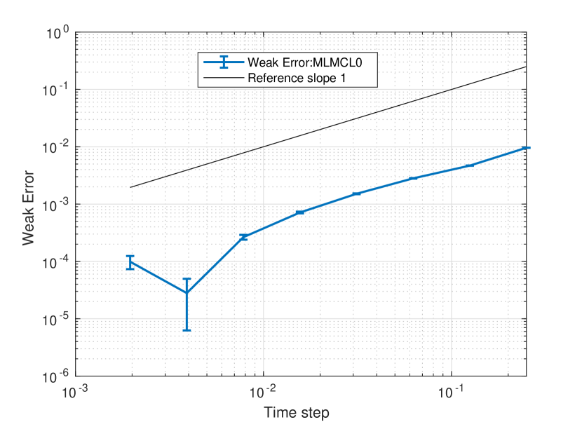
(a) MLMCL0

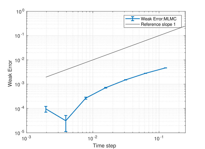
(b) MLMC

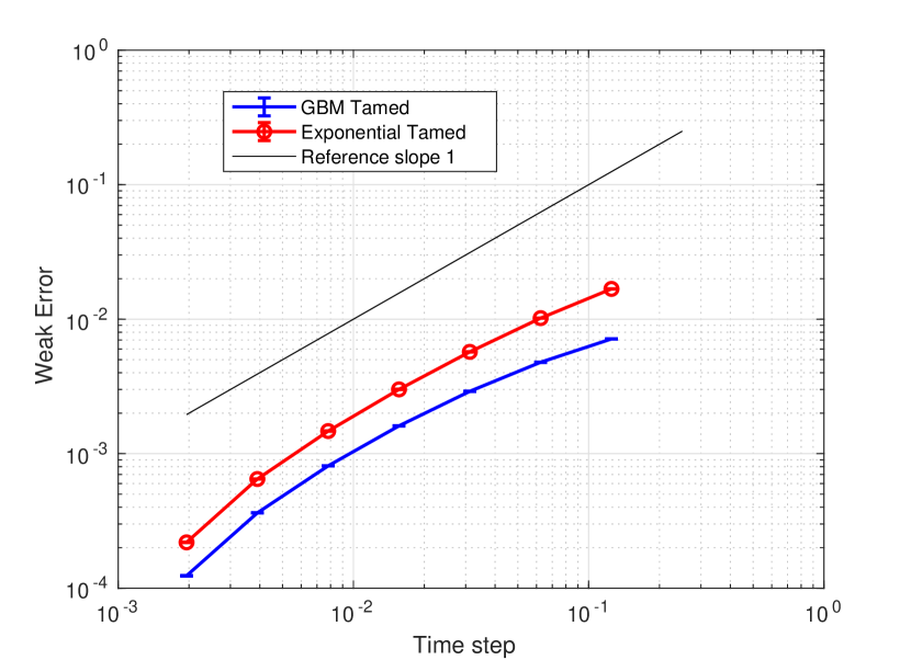
(c) MLMCSR

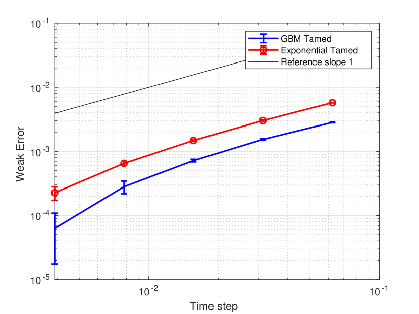
(d) Trad

Figure 1. Comparison of different approaches to estimate the weak error for $d=1$ with $\beta_{1}=0.1$ and $\beta_{2}=0$.

In Figure 2 we show convergence for $d=4$ and observe the predicted convergence of rate 1. In (A), (B) and (C) we restrict the largest step so that $\Delta t<0.02$. For the exponential tamed method it was essential to impose this restriction on the maximum step size as, although solutions remain bounded, the error is too large to observe convergence. These large solutions also lead to large variances and hence an infeasible large number of samples, (see also the discussion in [1]). This is illustrated by comparing (C) where we restrict $\Delta t<0.02$ and (D) where $\Delta t<0.2$. The exponential tamed method only starts to converge for $\Delta t\leq 0.02$. For the larger stepsizes in (D) we see the GBM based method performs well (unlike the exponential tamed method). The small step size restriction on the standard exponential method as $d$ increases makes it difficult to obtain a reference solution using this method using the MLMC method.

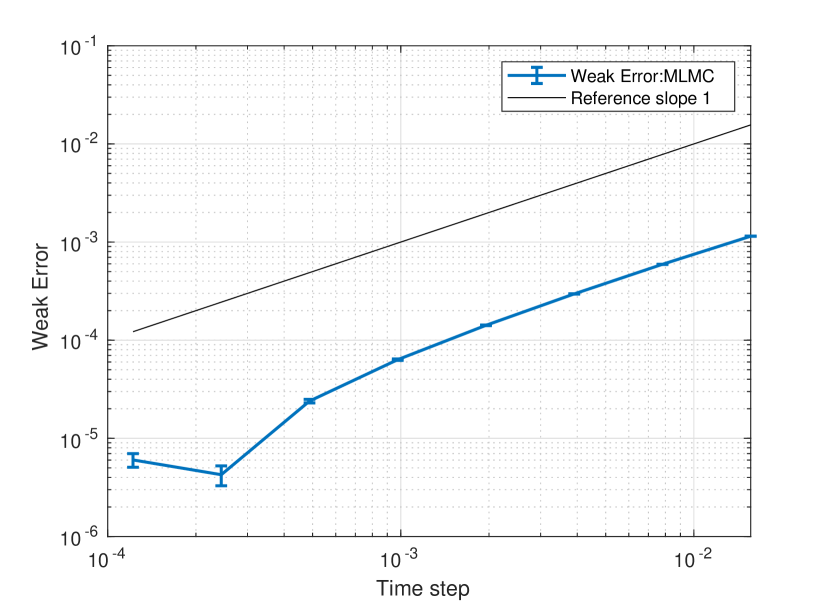
(a) MLMCL0

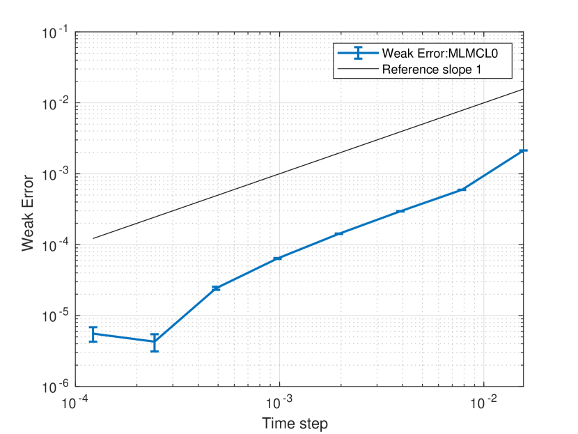
(b) MLMC

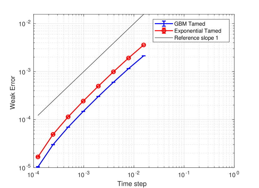
(c) MLMCSR ($\Delta t<0.02$)

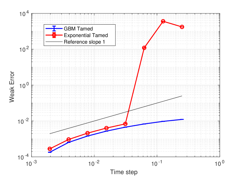
(d) MLMCSR ($\Delta t<0.2$)

Figure 2. Comparison of 3 different approaches to estimate the weak error for $d=4$ with $\beta_{1}=0.1$ and $\beta_{2}=0$. In (D) we see that the exponential tamed method is not well behaved for large time steps.

In Figure 3 we illustrate convergence using MLMCSR for the two methods with $d=50$ and $d=100$. We only examine MLMCSR as for these larger values of $d$ due to unreliable results the exponential tamed method for larger $\Delta t$ values (as discussed for Figure 2). We see that for $d=50$ we require $\Delta t<2\times 10^{-4}$ and for $d=100$ that $\Delta t<10^{-4}$ to obtain an approximation using the standard exponential tamed method. However, we observe that the GBM method converges with the predicted order and there is no issue with large variances.

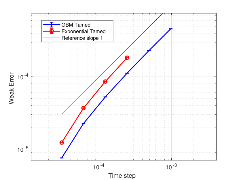
(a) MLMCSR $d=50$

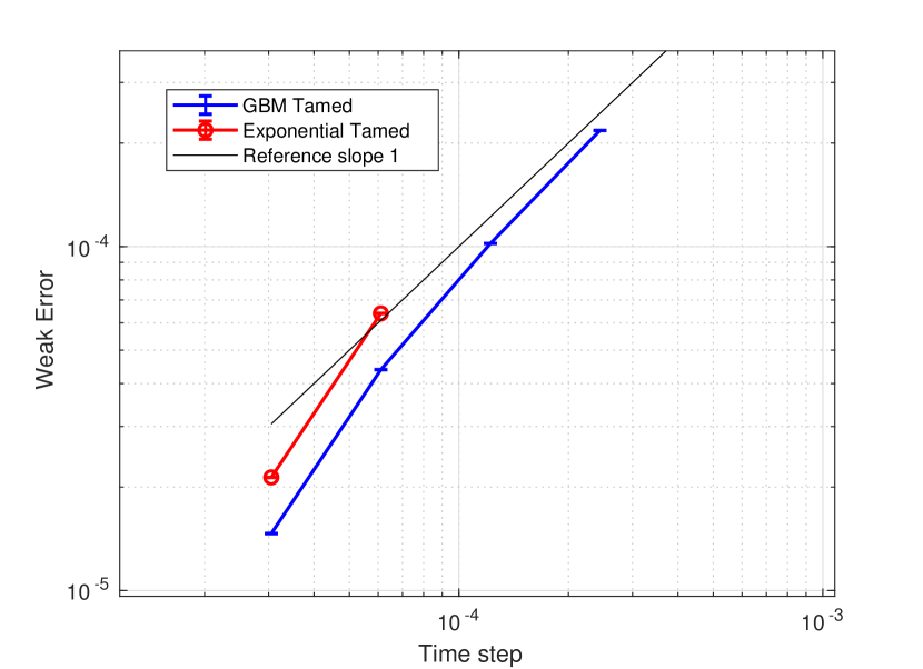
(b) MLMCSR $d=100$

Figure 3. Convergence for $d=50$ and $d=100$ with $\beta_{1}=0.1$ and $\beta_{2}=0$. For larger timesteps the exponential tamed method has a large variance and we do not see convergence until smaller timesteps.

For the nonlinear diffusion, with $\beta_{1}=\beta_{2}=0.1$ in (3), we illustrate convergence in Fig (4) (a) MLMCSR and (b) Trad. We have taken $d=4$ and observe weak convergence of rate one. Both the methods MLMC and MLMCL0 also show rate one convergence with the GBM based method having a smaller error constant. For this nonlinear noise, for larger values of $\Delta t$, although the taming ensures solutions remain bounded the variance does not reduce. This is now for both methods.

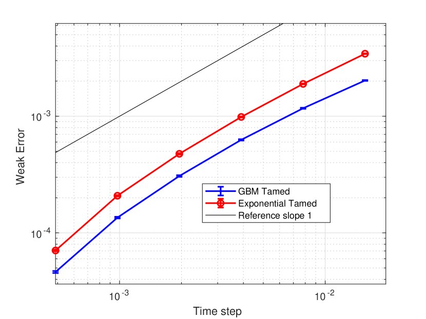
(a) MLMCSR

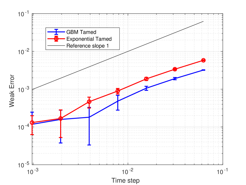
(b) Trad

Figure 4. Weak convergence for $d=4$ with $\beta_{1}=\beta_{2}=0.1$. We observe rate one convergence. A time step restriction is required.

4. Proof of Bounded Moments

We let $\Delta\mathbf{W}_{k}:=(\Delta W_{k}^{1},\Delta W_{k}^{2},\ldots,\Delta W_{k}^{m})^{T}.$ For the drift we define the notation

(17) $$\mathcal{N}(x):=F^{tm}_{\Delta t}(x)-\sum_{i=1}^{m}B_{i}g_{i}(x)$$

where $F^{tm}_{\Delta t}$ is defined in (8). We can use $\mathcal{N}$ to re-write (7) as

$$Y_{n+1}^{N}=\mathbf{\Phi}_{t_{n+1},t_{n}}\left(Y_{n}^{N}+\mathcal{N}(Y_{n}^{N})\Delta t+\sum_{i=1}^{m}g_{i}(Y_{n}^{N})\Delta W^{i}_{n}\right).$$

We now state the boundedness of the operator $\mathbf{\Phi}_{t,t_{0}}$ in stochastic $L^{p}$ spaces.

Lemma 2.

Suppose $p\geq 2$, $0\leq s<t\leq T$ and let $\mathbf{\Phi}_{t,s}$ be given in (6) with $t_{0}=s$. Then,

• For any $\mathcal{F}_{s}$ measurable random variable $v$ in $L^{p}(\Omega,\mathbb{R}^{d})$

  $$\left\lVert\mathbf{\Phi}_{t,s}v\right\rVert_{L^{p}(\Omega,\mathbb{R}^{d})}\leq\exp{\left(\left(\left\lVert A\right\rVert+\frac{p-1}{2}\sum_{i=1}^{m}\left\lVert B_{i}\right\rVert^{2}\right)(t-s)\right)}\left\lVert v\right\rVert_{L^{p}(\Omega,\mathbb{R}^{d})}.$$

• There are constants $\kappa_{1,2}>0$, independent of $(t-s)$ such that

  $$\mathbb{E}\left[\left\lVert\mathbf{\Phi}_{t,s}\right\rVert^{p}\right]\leq\kappa_{1}\exp(\kappa_{2}(t-s)).$$

Proof.

For the proof of $i)$, see [10]. To show $ii)$, we have

(18) $$\left\lVert\mathbf{\Phi}_{t,s}\right\rVert^{p}\leq\exp\left(\left\lVert p(A-\frac{1}{2}\sum_{i=1}^{m}B_{i}^{2})(t-s)\right\rVert\right)\exp\left(p\sum_{i=1}^{m}\left\lVert B_{i}\right\rVert|W_{t}^{i}-W_{s}^{i}|\right).$$

By taking expected value and considering the independence and distribution of random values $|W_{t}^{i}-W_{s}^{i}|$, for $i=1,2,\ldots,m$, we have

$$\mathbb{E}\left[\left\lVert\mathbf{\Phi}_{t,s}\right\rVert\right]^{p}$$

$$\leq \exp\left(\left\lVert p(A-\frac{1}{2}\sum_{i=1}^{m}B_{i}^{2})(t-s)\right\rVert\right)\prod_{i=1}^{m}\mathbb{E}\left[\exp\left(p\left\lVert B_{i}\right\rVert|W_{t}^{i}-W_{s}^{i}|\right)\right]$$

$$= \exp\left(\left\lVert p(A-\frac{1}{2}\sum_{i=1}^{m}B_{i}^{2})(t-s)\right\rVert\right)\prod_{i=1}^{m}\exp(p^{2}\left\lVert B_{i}\right\rVert^{2}(t-s))\left(1+\text{erf}(\frac{p\sqrt{t-s}\left\lVert B_{i}\right\rVert}{\sqrt{2}})\right).$$

By the boundedness of the function erf, the positive constants $\kappa_{1}$ and $\kappa_{2}$ are determined in terms of $p,\left\lVert A\right\rVert$ and $\left\lVert B_{i}\right\rVert$. ∎

For the proof Theorem 1, we adapt the approach given in [13] and we start by introducing appropriate sub events of $\Omega$. We let $\Omega_{0}^{N}:=\Omega$, then for $n\in\mathbb{N}_{N}^{+}$

$$\Omega_{n}^{N}:=\left\{\omega\in\Omega|,\sup_{k\in\mathbb{N}_{n-1}}D_{k}^{N}(\omega)\leq N^{1/4r},\sup_{k\in\mathbb{N}_{n-1}}\left\lVert\Delta\mathbf{W}_{k}\right\rVert\leq 1\right\},$$

where the parameter $r$ is defined in Assumption 1. The dominating stochastic process is defined by $D_{0}^{N}:=\left(\lambda+\left\lVert X_{0}\right\rVert\right)e^{\lambda}$ and for $n\in\mathbb{N}_{N}^{+}$

$$D_{n}^{N}:=(\lambda+\left\lVert X_{0}\right\rVert)\sup_{u\in\mathbb{N}_{n}}\prod_{k=u}^{n-1}\left\lVert\mathbf{\Phi}_{t_{k+1}},t_{k}\right\rVert\exp\left(\lambda+\sup_{u\in\mathbb{N}_{n}}\sum_{k=u}^{n-1}\left(\lambda\left\lVert\Delta\mathbf{W}_{k}\right\rVert^{2}+\beta_{k}^{N}\right)\right)$$

where

$$\beta_{k}^{N}:=\mathbbm{1}_{\left\lVert Y_{k}^{N}\right\rVert\geq 1}\frac{{{\big{\langle}}Y_{k}^{N},\sum_{i=1}^{m}g_{i}(Y_{k}^{N})\Delta W^{i}_{k}{\big{\rangle}}}}{\left\lVert Y_{k}^{N}\right\rVert^{2}}\quad\text{and}\quad\lambda:=\max\{\lambda_{0},\lambda_{1},\lambda_{2},\lambda_{3},\lambda_{4}\}.$$

Here $\lambda_{0},\ldots,\lambda_{4}$ are constants defined by

$$\lambda {}_{0}:=\exp\left({\sum_{i=1}^{m}\left\lVert B_{i}\right\rVert+T\left\lVert A-\frac{1}{2}\sum\limits_{i=1}^{m}B_{i}^{2}\right\rVert}\right)$$

$$\times\left(1+2TK+T\left\lVert F(0)\right\rVert+\sum_{i=1}^{m}\left\lVert B_{i}\right\rVert TK+T\left\lVert\sum_{i=1}^{m}B_{i}g_{i}(0)\right\rVert+mK+\sum_{i=1}^{m}\left\lVert g_{i}(0)\right\rVert\right)$$

$$\lambda_{1}: =m\sum_{i=1}^{m}\left(K+\left\lVert g_{i}(0)\right\rVert\right)^{2}$$

$$\lambda_{2}: =\left(2K+\left\lVert F(0)\right\rVert\right)^{4}$$

$$\lambda_{3}: =\left(\sum_{i=1}^{m}\left\lVert B_{i}\right\rVert K+\left\lVert\sum_{i=1}^{m}B_{i}g_{i}(0)\right\rVert\right)^{4}$$

$$\lambda_{4}: =\left(4T^{2}+2T\right)^{2},$$

and the constant $K$ is from Assumption 1. The first result shows we can dominate the numerical solution on the set $\Omega_{n}^{N}$.

Lemma 3.

Let Assumption 1 hold. Let $Y_{n}^{N}$ be given by (7) and let (9) hold. For all $n\in\mathbb{N}_{N}$ we have

$$1_{\Omega_{n}^{N}}\left\lVert Y_{n}^{N}\right\rVert\leq D_{n}^{N}.$$

Proof.

On $\Omega_{n+1}^{N}$ by construction $\left\lVert\Delta\mathbf{W}_{n}\right\rVert\leq 1$ for $n\in\mathbb{N}_{N-1}$. Therefore, $\left\lVert\mathbf{\Phi}_{t_{n+1},t_{n}}\right\rVert<\infty$ for $n\in\mathbb{N}_{N-1}$. We prove the Lemma on two subsets of $\Omega_{n+1}^{N}$

$$S^{(1)}_{n+1} :=\Omega_{n+1}^{N}\cap\{\omega\in\Omega|\left\lVert Y_{n}^{N}(\omega)\right\rVert\leq 1\}$$

$$S^{(2)}_{n+1} :=\Omega_{n+1}^{N}\cap\{\omega\in\Omega|1\leq\left\lVert Y_{n}^{N}(\omega)\right\rVert\leq N^{1/(4r)}\}.$$

First, on $S^{(1)}_{n+1}$, we have from (7) and the triangle inequality that

$$\left\lVert Y_{n+1}^{N}\right\rVert\leq\left\lVert\mathbf{\Phi}_{t_{n+1},t_{n}}\right\rVert\left(\left\lVert Y_{n}^{N}\right\rVert+\Delta t\left\lVert\mathcal{N}(Y_{n}^{N})\right\rVert+\sum_{i=1}^{m}\left\lVert g_{i}(Y_{n}^{N})\right\rVert\left\lVert\Delta\mathbf{W}_{n}\right\rVert\right).$$

Since $\left\lVert Y_{n}^{N}\right\rVert\leq 1$, $\left\lVert\Delta\mathbf{W}_{n}\right\rVert\leq 1$ on $S^{(1)}_{n+1}$, and by the taming inequality $\alpha(\Delta t,y)\leq 1$ from (9), we have that

$$\left\lVert Y_{n+1}^{N}\right\rVert\leq\left\lVert\mathbf{\Phi}_{t_{n+1},t_{n}}\right\rVert\left(1+\Delta t\left\lVert F(Y_{n}^{N})\right\rVert+\Delta t\left\lVert\sum_{i=1}^{m}B_{i}g_{i}(Y_{n}^{N})\right\rVert+\sum_{i=1}^{m}\left\lVert g_{i}(Y_{n}^{N})\right\rVert\right).$$

Adding and subtracting $F(0)$, $g_{i}(0)$ for $i=1,\ldots,m$, $\sum_{i=1}^{m}B_{i}g_{i}(0)$ and then applying the triangle inequality we get

$$\left\lVert Y_{n+1}^{N}\right\rVert\leq\left\lVert\mathbf{\Phi}_{t_{n+1},t_{n}}\right\rVert\Big{(}1+\Delta t\left\lVert F(Y_{n}^{N})-F(0)\right\rVert+\Delta t\left\lVert F(0)\right\rVert$$

$$+\Delta t\left\lVert\sum_{i=1}^{m}B_{i}g_{i}(Y_{n}^{N})-\sum_{i=1}^{m}B_{i}g_{i}(0)\right\rVert+\Delta t\left\lVert\sum_{i=1}^{m}B_{i}g_{i}(0)\right\rVert+\sum_{i=1}^{m}\left(\left\lVert g_{i}(Y_{n})-g_{i}(0)\right\rVert+\left\lVert g_{i}(0)\right\rVert\right)\Big{)}.$$

By Assumption 1 $(i)$, the global Lipschitz condition on $g_{i}$, and using that $\Delta t\leq T$

$$\left\lVert Y_{n+1}^{N}\right\rVert\leq \left\lVert\mathbf{\Phi}_{t_{n+1},t_{n}}\right\rVert\Big{(}1+TK\left(1+\left\lVert Y_{n}^{N}\right\rVert^{2r}\right)\left\lVert Y_{n}^{N}\right\rVert+T\left\lVert F(0)\right\rVert+TK\sum_{i=1}^{m}\left\lVert B_{i}\right\rVert\left\lVert Y_{n}^{N}\right\rVert$$

$$+T\left\lVert\sum_{i=1}^{m}B_{i}g_{i}(0)\right\rVert+mK\left\lVert Y_{n}^{N}\right\rVert+\sum_{i=1}^{m}\left\lVert g_{i}(0)\right\rVert\Big{)}.$$

On $S^{(1)}_{n+1}$, since $\left\lVert Y_{n}^{N}\right\rVert\leq 1$ and $\left\lVert\Delta\mathbf{W}_{n}\right\rVert\leq 1$, we have

(19) $$\left\lVert Y_{n+1}^{N}\right\rVert\leq\lambda.$$

To obtain an inequality on $S^{(2)}_{n+1}$, we start from (7) by squaring the norm

$$\left\lVert Y_{n+1}^{N}\right\rVert^{2}\leq\left\lVert\mathbf{\Phi}_{t_{n+1},t_{n}}\right\rVert^{2}\left\lVert Y_{n}^{N}+\Delta t\mathcal{N}(Y_{n}^{N})+\sum_{i=1}^{m}g_{i}(Y_{n}^{N})\Delta W^{i}_{n})\right\rVert^{2}$$

$$\leq\left\lVert\mathbf{\Phi}_{t_{n+1},t_{n}}\right\rVert^{2}\left(\left\lVert Y_{n}^{N}\right\rVert^{2}+\Delta t^{2}\left\lVert\mathcal{N}(Y_{n}^{N})\right\rVert^{2}+m\sum_{i=1}^{m}\left\lVert g_{i}(Y_{n}^{N})\right\rVert^{2}\left\lVert\Delta\mathbf{W}_{n}\right\rVert^{2}\right.$$

$$\left.+2\Delta t{\big{\langle}}Y_{n}^{N},\mathcal{N}(Y_{n}^{N}){\big{\rangle}}+2{\big{\langle}}Y_{n}^{N},\sum_{i=1}^{m}g_{i}(Y_{n}^{N})\Delta W^{i}_{n}{\big{\rangle}}+2\Delta t{\big{\langle}}\mathcal{N}(Y_{n}^{N}),\sum_{i=1}^{m}g_{i}(Y_{n}^{N})\Delta W^{i}_{n}{\big{\rangle}}\right).$$

Applying the Cauchy-Schwarz and Arithmetic-Geometric inequalities

$$\left\lVert Y_{n+1}^{N}\right\rVert^{2} \leq\left\lVert\mathbf{\Phi}_{t_{n+1},t_{n}}\right\rVert^{2}\left(\left\lVert Y_{n}^{N}\right\rVert^{2}+2\Delta t^{2}\left\lVert\mathcal{N}(Y_{n}^{N})\right\rVert^{2}+2m\sum_{i=1}^{m}\left\lVert g_{i}(Y_{n}^{N})\right\rVert^{2}\left\lVert\Delta\mathbf{W}_{n}\right\rVert^{2}\right.$$

(20) $$\left.+2\Delta t{\big{\langle}}Y_{n}^{N},\mathcal{N}(Y_{n}^{N}){\big{\rangle}}+2{\big{\langle}}Y_{n}^{N},\sum_{i=1}^{m}g_{i}(Y_{n}^{N})\Delta W^{i}_{n}{\big{\rangle}}\right).$$

Let us consider $\mathcal{N}(Y_{n}^{N})$ (see (17)). Following the argument in [13, (40) in Proof of Lemma 3.1] we have

$$\left\lVert F(Y_{n}^{N})\right\rVert^{2}\leq N\sqrt{\lambda}\left\lVert Y_{n}^{N}\right\rVert^{2}.$$

Further, by Assumption 1 $(v)$, the global Lipschitz property of the function $g_{i}$

(21) $$\left\lVert\sum_{i=1}^{m}B_{i}g_{i}(Y_{n}^{N})\right\rVert^{2} \leq\left(\sum_{i=1}^{m}\left\lVert B_{i}\right\rVert K+\left\lVert\sum_{i=1}^{m}B_{i}g_{i}(0)\right\rVert\right)^{2}\left\lVert Y_{n}^{N}\right\rVert^{2}$$

$$\leq\sqrt{\lambda}\left\lVert Y_{n}^{N}\right\rVert^{2}$$

and

$$\left\lVert g_{i}(Y_{n}^{N})\right\rVert^{2}\leq\left(K+\left\lVert g_{i}(0)\right\rVert\right)^{2}\left\lVert Y_{n}^{N}\right\rVert^{2}.$$

By definition of $\lambda$, we have

$$m\sum_{i}^{m}\left\lVert g_{i}(Y_{n}^{N})\right\rVert^{2}\leq\lambda\left\lVert Y_{n}^{N}\right\rVert^{2}.$$

Therefore the linear growth of the second term on the RHS of (4)

$$\left\lVert\mathcal{N}(Y_{n}^{N})\right\rVert^{2}\leq 4N\sqrt{\lambda}\left\lVert Y_{n}^{N}\right\rVert^{2}$$

on $S^{(2)}_{n+1}$ is obtained. The one sided Lipschitz condition on $F$ given in (4) and the Cauchy–Schwarz inequality give that

(22) $${\big{\langle}}Y_{n}^{N},F(Y_{n}^{N}){\big{\rangle}} \leq{\big{\langle}}Y_{n}^{N},F(Y_{n}^{N})-F(0){\big{\rangle}}+{\big{\langle}}Y_{n}^{N},F(0){\big{\rangle}}$$

(23) $$\leq\left(K+\left\lVert F(0)\right\rVert\right)\left\lVert Y_{n}^{N}\right\rVert^{2}$$

(24) $$\leq\sqrt{\lambda}\left\lVert Y_{n}^{N}\right\rVert^{2}$$

where we have used that $1\leq\|Y_{n}^{N}\|$. Therefore by the inequalities (21), (22), Cauchy-Schwarz inequality for the term ${\big{\langle}}Y_{n}^{N},\sum_{i=1}^{m}B_{i}g_{i}(Y_{n}^{N}){\big{\rangle}}$ and $\lambda>1$

$${\big{\langle}}Y_{n}^{N},\mathcal{N}(Y_{n}^{N}){\big{\rangle}} =\alpha(\Delta t,Y_{n}^{N}){\big{\langle}}Y_{n}^{N},F(Y_{n}^{N}){\big{\rangle}}-{\big{\langle}}Y_{n}^{N},\sum_{i=1}^{m}B_{i}g_{i}(Y_{n}^{N}){\big{\rangle}}$$

$$\leq\left(\alpha(\Delta t,Y_{n}^{N})+1\right)\sqrt{\lambda}\left\lVert Y_{n}^{N}\right\rVert^{2}.$$

As a result, since $\Delta t=T/N$, $\alpha(\Delta t,Y_{n}^{N})<1$, by (9), and $(4T^{2}+2T)\leq\sqrt{\lambda}$, we see that on $S^{(2)}_{n+1}$ (4) becomes

$$\left\lVert Y_{n+1}^{N}\right\rVert^{2} \leq\left\lVert\mathbf{\Phi}_{t_{n+1},t_{n}}\right\rVert^{2}\left\lVert Y_{n}^{N}\right\rVert^{2}\left(1+\frac{8T^{2}}{N}\sqrt{\lambda}+2\lambda\left\lVert\Delta\mathbf{W}_{n}\right\rVert^{2}+\frac{4T}{N}\sqrt{\lambda}+2\beta_{n}^{N}\right)$$

$$\leq\left\lVert\mathbf{\Phi}_{t_{n+1},t_{n}}\right\rVert^{2}\left\lVert Y_{n}^{N}\right\rVert^{2}\left(1+\frac{2\lambda}{N}+2\lambda\left\lVert\Delta\mathbf{W}_{n}\right\rVert^{2}+2\beta_{n}^{N}\right)$$

(25) $$\leq\left\lVert\mathbf{\Phi}_{t_{n+1},t_{n}}\right\rVert^{2}\left\lVert Y_{n}^{N}\right\rVert^{2}\exp\left(\frac{2\lambda}{N}+2\lambda\left\lVert\Delta\mathbf{W}_{n}\right\rVert^{2}+2\beta_{n}^{N}\right).$$

Now we carry out an induction argument on $n$. The case for $n=0$ is obvious by initial condition on $\Omega_{0}^{N}=\Omega$. Let $l\in\mathbb{N}_{N-1}$ and assume $\left\lVert Y_{n}^{N}(\omega)\right\rVert\leq D_{n}^{N}(\omega)$ holds for all $n\in\mathbb{N}_{l}$ where $\omega\in\Omega_{n}^{N}$. We now prove that

$$\left\lVert Y_{l+1}^{N}(\omega)\right\rVert\leq D_{l+1}^{N}(\omega)\quad\text{for all}\quad\omega\in\Omega_{l+1}^{N}.$$

For all $\omega\in\Omega_{l+1}^{N}$, we have by the induction hypothesis $\left\lVert Y_{n}^{N}(\omega)\right\rVert\leq D_{n}^{N}(\omega)\leq N^{1/(4r)}$, $n\in\mathbb{N}_{l}$ and $\Omega_{l+1}^{N}\subseteq\Omega_{n+1}^{N}$. For any $\omega\in\Omega_{l+1}^{N}$, $\omega$ belongs to $S_{n+1}^{(1)}$ or $S_{n+1}^{(2)}$. For the inductive argument we define a random variable

$$\tau_{l}^{N}(\omega):=\max\left(\{-1\}\cup\{n\in\mathbb{N}_{l-1}\}\bigg{|}\left\lVert Y_{n}^{N}(\omega)\right\rVert\leq 1\}\right)$$

as in [13]. This definition implies that $1\leq\left\lVert Y_{n}^{N}(\omega)\right\rVert\leq N^{1/(4r)}$ for all $n\in\{\tau_{l+1}^{N}(\omega)+1,\tau_{l+2}^{N}(\omega),\ldots,l\}$. By the bound in (4)

$$\left\lVert Y_{l+1}^{N}(\omega)\right\rVert\leq\left\lVert\mathbf{\Phi}_{t_{l+1},t_{l}}(\omega)\right\rVert\left\lVert Y_{l}^{N}(\omega)\right\rVert\exp\left(\frac{\lambda}{N}+\lambda\left\lVert\Delta\mathbf{W}_{l}(\omega)\right\rVert^{2}+\beta_{l}^{N}(\omega)\right)$$

$$\leq\left\lVert Y_{\tau_{l+1}^{N}(\omega)+1}^{N}(\omega)\right\rVert$$

$$\times\prod_{n=\tau_{l+1}^{N}(\omega)+1}^{l}\left(\left\lVert\mathbf{\Phi}_{t_{n+1},t_{n}}(\omega)\right\rVert\right)\exp\left(\sum_{n=\tau_{l+1}+1}^{l}\left(\frac{\lambda}{N}+\lambda\left\lVert\Delta\mathbf{W}_{n}(\omega)\right\rVert^{2}+\beta_{n}^{N}(\omega)\right)\right)$$

$$\leq\left\lVert Y_{\tau_{l+1}^{N}(\omega)+1}^{N}(\omega)\right\rVert$$

$$\sup_{u\in\mathbb{N}_{l+1}}\times\prod_{n=u}^{l}\left\lVert\mathbf{\Phi}_{t_{n+1},t_{n}}(\omega)\right\rVert\exp\left(\lambda+\sup_{u\in\mathbb{N}_{l+1}}\sum_{n=u}^{l}\left(\lambda\left\lVert\Delta\mathbf{W}_{n}(\omega)\right\rVert^{2}+\beta_{n}^{N}(\omega)\right)\right).$$

By considering (19), the following completes the induction step and proof

$$\begin{split}&\left\lVert Y_{l+1}^{N}(\omega)\right\rVert\leq(\lambda+\left\lVert X_{0}(\omega)\right\rVert)\\ &\times\sup_{u\in\in\mathbb{N}_{l+1}}\prod_{n=u}^{l}\left\lVert\mathbf{\Phi}_{t_{n+1},t_{n}}(\omega)\right\rVert\exp\left(\lambda+\sup_{u\in\mathbb{N}_{l+1}}\sum_{n=u}^{l}\left(\lambda\left\lVert\Delta\mathbf{W}_{n}(\omega)\right\rVert^{2}+\beta_{n}^{N}(\omega)\right)\right)\\ &=D_{l+1}^{N}(\omega).\end{split}$$

∎

Lemma 4.

For all $p\geq 1$, $\sup_{N\in\mathbb{N}}\mathbb{E}\left[\sup_{n\in\mathbb{N}_{N}}|D_{n}^{N}|^{p}\right]<\infty.$

Proof.

By Hölder’s inequality, we have

$$\begin{split}&\mathop{\sup_{N\in\mathbb{N}}}_{N\geq 8\lambda pT}\left\lVert\sup_{n\in\mathbb{N}_{N}}D_{n}^{N}\right\rVert_{L^{p}(\Omega,\mathbb{R})}\leq e^{\lambda}\Big{(}\lambda+\left\lVert X_{0}\right\rVert_{L^{8p}(\Omega,\mathbb{R}^{d})}\Big{)}\\ &\times\mathop{\sup_{N\in\mathbb{N}}}_{N\geq 8\lambda pT}\left\lVert\prod_{k=0}^{N-1}\left\lVert\mathbf{\Phi}_{t_{k+1},t_{k}}\right\rVert\right\rVert_{L^{8p}(\Omega,\mathbb{R})}\left(\mathop{\sup_{N\in\mathbb{N}}}_{N\geq 8\lambda pT}\left\lVert\exp\sum_{k=0}^{N-1}\left(\lambda\left\lVert\Delta\mathbf{W}_{k}\right\rVert^{2}\right)\right\rVert_{L^{4p}(\Omega,\mathbb{R})}\right)\\ &\times\left(\sup_{N\in\mathbb{N}}\left\lVert\sup_{n\in\mathbb{N}_{N}}\exp\left(\sup_{u\in\mathbb{N}_{n}}\sum_{k=u}^{n-1}\ \beta_{k}^{N}\right)\right\rVert_{L^{4p}(\Omega,\mathbb{R})}\right).\end{split}$$

The boundedness of the third term on the RHS is due to the $\Delta t$ dependence of the upper bound of stochastic norm of $\left\lVert\mathbf{\Phi}_{t_{k+1},t_{k}}\right\rVert$ given in Lemma 2 . On the other hand, the last two terms are shown to be bounded in [13, Lemma 3.5]. ∎

Lemma 5.

Let $\bar{Y}_{t}$ be given by (11). For all $p\geq 1$, there exists $K=K(T)>0$ such that

$$\left\lVert\bar{Y}_{t}\right\rVert_{L^{p}(\Omega,\mathbb{R}^{d})}^{2}\leq K\left(1+\left\lVert\bar{Y}_{t_{n}}\right\rVert_{L^{p}(\Omega,\mathbb{R}^{d})}^{2}\right).$$

Proof.

Follows since $\bar{Y}_{t}$ is the solution to a linear SDE with initial condition $\bar{Y}_{t_{n}}$ on the interval $[t_{n},t]$. ∎

We now use these Lemmas to prove the scheme has bounded moments.

Proof of Theorem 1: Bounded moments

Proof.

Consider the Itô equation for continuous extension of numerical solution given in Lemma (1) on $[0,t]$

$$\bar{Y}_{t_{n}}=X_{0}+\sum_{k=0}^{n-1}\int_{t_{k}}^{t_{k+1}}\left(A\bar{Y}_{s}+\mathbf{\Phi}_{s,t_{k}}\alpha(\Delta t,\bar{Y}_{t_{k}})F(\bar{Y}_{t_{k}})\right)ds\\ +\sum_{k=0}^{n-1}\sum_{i=1}^{m}\int_{t_{k}}^{t_{k+1}}\left(B_{i}\bar{Y}_{s}+\mathbf{\Phi}_{s,t_{k}}g_{i}(\bar{Y}_{t_{k}})\right)dW_{s}^{i}.$$

By adding and subtracting the terms $\sum_{i=1}^{m}\sum_{k=0}^{n-1}\int_{t_{k}}^{t_{k+1}}\mathbf{\Phi}_{s,t_{k}}B_{i}g_{i}(0)ds$, $\sum_{k=0}^{n-1}\int_{t_{k}}^{t_{k+1}}\mathbf{\Phi}_{s,t_{k}}g_{i}(0)dW_{s}^{i}$ and using the triangle inequality, we have

$$\left\lVert\bar{Y}_{t_{n}}\right\rVert_{L^{p}(\Omega,\mathbb{R}^{d})} \leq\left\lVert X_{0}\right\rVert_{L^{p}(\Omega,\mathbb{R}^{d})}+\left\lVert A\right\rVert\sum_{k=0}^{n-1}\int_{t_{k}}^{t_{k+1}}\left\lVert\bar{Y}_{s}\right\rVert_{L^{p}(\Omega,\mathbb{R}^{d})}ds$$

$$+\sum_{k=0}^{n-1}\int_{t_{k}}^{t_{k+1}}\left\lVert\mathbf{\Phi}_{s,t_{k}}\alpha(\Delta t,\bar{Y}_{t_{k}})F(\bar{Y}_{t_{k}})\right\rVert_{L^{p}(\Omega,\mathbb{R}^{d})}ds$$

$$+\left\lVert\sum_{k=0}^{n-1}\int_{t_{k}}^{t_{k+1}}\sum_{i=1}^{m}B_{i}\bar{Y}_{s}dW_{s}^{i}\right\rVert_{L^{p}(\Omega,\mathbb{R}^{d})}$$

$$+\left\lVert\sum_{k=0}^{n-1}\int_{t_{k}}^{t_{k+1}}\mathbf{\Phi}_{s,t_{k}}\sum_{i=1}^{m}g_{i}(0)dW_{s}^{i}\right\rVert_{L^{p}(\Omega,\mathbb{R}^{d})}$$

$$+\left\lVert\sum_{k=0}^{n-1}\int_{t_{k}}^{t_{k+1}}\mathbf{\Phi}_{s,t_{k}}\sum_{i=1}^{m}\left(g_{i}(\bar{Y}_{t_{k}})-g_{i}(0)\right)dW_{s}^{i}\right\rVert_{L^{p}(\Omega,\mathbb{R}^{d})}.$$

By Lemma 2, that $\left\lVert\alpha(\Delta t,\bar{Y}_{t_{k}})F(\bar{Y}_{t_{k}})\Delta t\right\rVert\leq 1$ in (9), along with the Burkholder-Davis-Gundy Inequality (see [22]) we have

$$\begin{split}\left\lVert\bar{Y}_{t_{n}}\right\rVert_{L^{p}(\Omega,\mathbb{R}^{d})}&\leq\left\lVert X_{0}\right\rVert_{L^{p}(\Omega,\mathbb{R}^{d})}+\left\lVert A\right\rVert\left\lVert\sum_{k=0}^{n-1}\int_{t_{k}}^{t_{k+1}}\bar{Y}_{s}\right\rVert_{L^{p}(\Omega,\mathbb{R}^{d})}ds+KN\\ &+p\left(\sum_{k=0}^{n-1}\int_{t_{k}}^{t_{k+1}}\sum_{i=1}^{m}\left\lVert B_{i}\bar{Y}_{s}\right\rVert_{L^{p}(\Omega,\mathbb{R}^{d})}^{2}ds\right)^{1/2}\\ &+pK\left(\sum_{i=1}^{m}\left\lVert g_{i}(0)\right\rVert^{2}T\right)^{1/2}+K^{2}\sqrt{m}p\left(\sum_{k=0}^{n-1}\int_{t_{k}}^{t_{k+1}}\left\lVert\bar{Y}_{t_{k}}\right\rVert_{L^{p}(\Omega,\mathbb{R}^{d})}^{2}ds\right)^{1/2}.\end{split}$$

By taking the square of both sides and applying the Jensen inequalities for sum and integrals

(26) $$\left\lVert\bar{Y}_{t_{n}}\right\rVert_{L^{p}(\Omega,\mathbb{R}^{d})}^{2} \leq 4\left(\left\lVert X_{0}\right\rVert_{L^{p}(\Omega,\mathbb{R}^{d})}+pK\left(\sum_{i=1}^{m}\left\lVert g_{i}(0)\right\rVert^{2}T\right)^{1/2}+KN\right)^{2}$$

$$+4\left\lVert A\right\rVert^{2}T\sum_{k=0}^{n-1}\int_{t_{k}}^{t_{k+1}}\left\lVert\bar{Y}_{s}\right\rVert_{L^{p}(\Omega,\mathbb{R}^{d})}^{2}ds$$

$$+4p^{2}\sum_{k=0}^{n-1}\int_{t_{k}}^{t_{k+1}}\sum_{i=1}^{m}\left\lVert B_{i}\bar{Y}_{s}\right\rVert_{L^{p}(\Omega,\mathbb{R}^{d})}^{2}ds$$

$$+4K^{4}mp^{2}\sum_{k=0}^{n-1}\int_{t_{k}}^{t_{k+1}}\left\lVert\bar{Y}_{t_{k}}\right\rVert_{L^{p}(\Omega,\mathbb{R}^{d})}^{2}ds.$$

Substituting (5) into (26) and rewriting the resulting integral inequality in discrete form, we have

$$\begin{split}&\left\lVert Y_{n}^{N}\right\rVert_{L^{p}(\Omega,\mathbb{R}^{d})}^{2}\leq 4\left(\left\lVert X_{0}\right\rVert_{L^{p}(\Omega,\mathbb{R}^{d})}+pK\left(\sum_{i=1}^{m}\left\lVert g_{i}(0)\right\rVert^{2}T\right)^{1/2}+KN\right)^{2}\\ &\quad+4\left\lVert A\right\rVert^{2}T\sum_{k=0}^{n-1}K(1+\left\lVert Y_{k}^{N}\right\rVert_{L^{p}(\Omega,\mathbb{R}^{d})}^{2})\frac{T}{N}\\ &\quad+4p^{2}\sum_{k=0}^{n-1}\sum_{i=1}^{m}\left\lVert B_{i}\right\rVert^{2}K(1+\left\lVert Y_{k}^{N}\right\rVert_{L^{p}(\Omega,\mathbb{R}^{d})}^{2})\frac{T}{N}+4K^{4}mp^{2}\sum_{k=0}^{n-1}\left\lVert Y_{k}^{N}\right\rVert_{L^{p}(\Omega,\mathbb{R}^{d})}^{2}\frac{T}{N}.\end{split}$$

By the discrete Gronwall inequality

$$\begin{split}\sup_{n\in\mathbb{N}_{N}}\left\lVert Y_{n}^{N}\right\rVert_{L^{p}(\Omega,\mathbb{R}^{d})}\leq C_{\left\lVert A\right\rVert,\left\lVert B_{i}\right\rVert,T,p,K}\left(\left\lVert X_{0}\right\rVert_{L^{p}(\Omega,\mathbb{R}^{d})}+pK\left(\sum_{i=1}^{m}\left\lVert g_{i}(0)\right\rVert^{2}T\right)^{1/2}\right.\\ \left.+KN+\left\lVert A\right\rVert T\sqrt{K}+p\sum_{i=1}^{m}\left\lVert B_{i}\right\rVert\sqrt{KT}\right).\end{split}$$

Following the bootstrap argument presented in [13, Lemma 3.9] to deal with the term $KN$ on the RHS, we get

(27) $$\sup_{N\in\mathbb{N}}\sup_{n\in\mathbb{N}_{N}}\left\lVert 1_{(\Omega_{n}^{N})^{c}}Y_{n}^{N}\right\rVert_{L^{p}(\Omega,\mathbb{R}^{d})}<\infty$$

and

(28) $$\mathop{\sup_{N\in\mathbb{N}}}_{N\geq 8\lambda pT}\sup_{n\in\mathbb{N}_{N}}\left\lVert 1_{\Omega_{n}^{N}}Y_{n}^{N}\right\rVert_{L^{p}(\Omega,\mathbb{R}^{d})}\leq\mathop{\sup_{N\in\mathbb{N}}}_{N\geq 8\lambda pT}\sup_{n\in\mathbb{N}_{N}}\left\lVert D_{n}^{N}\right\rVert_{L^{p}(\Omega,\mathbb{R}^{d})}.$$

The boundedness of the term in right hand side of (28) is proved in Lemma 4. Hence the proof is complete. ∎

5. Proof of Weak Convergence

For an SDE such as (1) with globally-Lipschitz drift and diffusion coefficients many classical textbooks on stochastic analysis consider the Kolmogorov PDE. However, for non-globally Lipschitz drift coefficients there are far fewer results. One key work is Cerrai [7] for the properties of the exact solution to a SDE with one-sided drift coefficient. To get order one weak convergence we need bounded moments of higher derivatives of the exact solution of the SDE (1) with respect to the initial condition. By the notation $X_{t}^{x}$, we emphasize that the initial condition is $X_{0}=x$. We denote the derivative of the exact solution with respect to the initial condition by $\mathbf{D}_{x}X_{t}^{x}$.

The following regularity result is given in [7] (see also [28]).

Lemma 6.

Let Assumption 1 hold and $X_{t}^{x}$ be the solution to (1). Then for $i=1,2,3,4$, $p\geq 1$ and $t\in[0,T]$

$$\sup_{x\in\mathbb{R}^{d}}\mathbb{E}\left[\left\lVert\mathbf{D}_{x}^{i}X_{t}^{x}\right\rVert^{p}\right]<\infty.$$

Before continuing we define two quantities.

(29) $$\Psi(t,x) :=\mathbb{E}\left[\phi(X_{t})|X_{0}=x\right]=\mathbb{E}\left[\phi(X_{t}^{x})\right]$$

(30) $$u(t,\bar{Y}_{t}) :=\Psi_{T-t}(\bar{Y}_{t}).$$

Lemma 7.

Let $X_{t}$ be the solution to (1). Suppose that $\phi:\mathbb{R}^{d}\to\mathbb{R}$ and $\phi\in C^{2}_{b}(\mathbb{R}^{d})$. Then, $\Psi(t,x)$ defined in (29) satisfies the Kolmogorov PDE

$$\frac{\partial}{\partial t}\Psi(t,x)=\mathcal{L}\Psi(t,x)$$

where

$$\mathcal{L}\Psi(t,x):=\mathbf{D}\Psi(t,x)\mu(x)+\frac{1}{2}\sum_{i=1}^{m}\sigma_{i}(x)^{\intercal}\mathbf{D}^{2}\Psi(t,x)\sigma_{i}(x).$$

Proof.

Cerrai [7] imposes the conditions (Hypothesis 1.1 and 1.2 in [7]) which are implied by our Assumption 1. On the other hand, the function $\phi$ is only assumed to be in $C_{b}(\mathbb{R}^{d})$ in [7]. To show that $\Psi(t,x)\in C^{2}_{b}(\mathbb{R}^{d})$ and $\Psi(t,x)$ is solution to (7), an extra hypothesis (Hypothesis 1.3) is imposed on the diffusion coefficient. Here, we directly assume that $\phi$ is in $C^{2}_{b}(\mathbb{R}^{d})$. We note that the global Lipschitz assumption of Assumption 1 $(v)$ for the diffusion term is far stronger than in [7] and hence simplifies many steps in the proof. ∎

Although in Lemma 7 we have $\phi\in C^{2}_{b}(\mathbb{R}^{d})$, to get the correct order of weak convergence, we impose $\phi\in C^{4}_{b}(\mathbb{R}^{d})$ in Theorem 2. We now take $C$ as a generic constant that is independent of the time step $\Delta t$.

Corollary 1.

For each $T>0$, there exists $C>0$ such that for $0\leq t\leq T$

(31) $$|\mathbb{E}\left[\mathbf{D}\Psi(t,x)\xi\right]|\leq C\left\lVert\mathbb{E}\left[\xi\right]\right\rVert,\qquad\text{for all }\xi\in L^{p}(\Omega,\mathbb{R}^{d}),\quad p\geq 1.$$

Proof.

By interchanging the derivative and expectation (see discussion in [4, sections 5.1 and 5.2]), the chain rule and the definition of $\Psi$ in (29)

$$|\mathbb{E}\left[\mathbf{D}\Psi(t,x)\xi\right]| =|\mathbf{D}\Psi(t,x)\mathbb{E}\left[\xi\right]|$$

$$=|\mathbb{E}\left[\mathbf{D}\phi(X_{t}^{x})\mathbf{D}_{x}X_{t}^{x}\right]\mathbb{E}\left[\xi\right]|.$$

Then by the deterministic Cauchy-Schwarz and triangle inequality

$$|\mathbb{E}\left[\mathbf{D}\Psi(t,x)\xi\right]| \leq\left\lVert\mathbb{E}\left[\mathbf{D}\phi(X_{t}^{x})\mathbf{D}_{x}X_{t}^{x}\right]\right\rVert\left\lVert\mathbb{E}\left[\xi\right]\right\rVert$$

$$\leq\mathbb{E}\left[\left\lVert\mathbf{D}\phi(X_{t}^{x})\mathbf{D}_{x}X_{t}^{x}\right\rVert\right]\left\lVert\mathbb{E}\left[\xi\right]\right\rVert$$

$$\leq\mathbb{E}\left[\left\lVert\mathbf{D}\phi(X_{t}^{x})\right\rVert^{2}\right]^{1/2}\mathbb{E}\left[\left\lVert\mathbf{D}_{x}X_{t}^{x}\right\rVert^{2}\right]^{1/2}\left\lVert\mathbb{E}\left[\xi\right]\right\rVert$$

where on the last step we used the stochastic Cauchy-Schwarz inequality. The bounded derivatives condition on $\phi$, and Lemma 6 complete the proof. ∎

We point out inequality (31) implies, for $u$ defined in (30), that

$$|\mathbb{E}\left[\mathbf{D}u(s,\bar{Y}_{s})\xi\right]|\leq C\left\lVert\mathbb{E}\left[\xi\right]\right\rVert$$

where $\xi$ is a $\mathbb{R}^{d}$ -valued random variable. With these preliminary results we are now in a position to prove weak convergence.

Proof of Theorem 2: weak convergence

Proof.

Recall the definition of $\Psi(t,x)$ from (29). Applying the Itô formula on $[t_{n},t_{n+1})$ for $\Psi(t,\bar{Y}_{t})$ with $\bar{Y}_{t}$ given by (1) gives

$$d\Psi(t,\bar{Y}_{t})=\left(\frac{\partial}{\partial t}+\mathcal{\hat{L}}_{n}(t)\right)\Psi(t,\bar{Y}_{t})dt+\sum_{i=1}^{m}\mathcal{\hat{L}}^{i}_{n}(t)\Psi(t,\bar{Y}_{t})dW^{i}_{t}$$

where

$$\begin{split}\mathcal{\hat{L}}_{n}(t)\Psi(t,\bar{Y}_{t})&:=\mathbf{D}\Psi(t,\bar{Y}_{t})\mu^{tm}(t,t_{n})+\frac{1}{2}\sum_{i=1}^{m}\sigma_{i}^{tm}(t,t_{n})^{\intercal}\mathbf{D}^{2}\Psi(t,\bar{Y}_{t})\sigma_{i}^{tm}(t,t_{n})\\ \mathcal{\hat{L}}^{i}_{n}(t)\Psi(t,\bar{Y}_{t})&:=\mathbf{D}\Psi(t,\bar{Y}_{t})\sigma_{i}^{tm}(t,t_{n})\end{split}$$

and $\mu^{tm}$ and $\sigma_{i}^{tm}$ are defined in (1). Now we define the error function $e$ by

$$e:=|\Psi_{0}(\bar{Y}_{T})-\Psi_{T}(\bar{Y}_{0})|=\bigg{|}\mathbb{E}\left[\phi(\bar{Y}_{T})-\phi(X_{T})|X_{0}=x\right]\bigg{|}.$$

By definition of $u$ in (30) and the fundamental theorem of calculus for the deterministic function $u$

$$e=|u(T,\bar{Y}_{T})-u(0,\bar{Y}_{0})|=\Big{|}\int_{0}^{T}d(u(s,\bar{Y}_{s}))\Big{|}=\Big{|}\sum_{k=0}^{N-1}\int_{s=t_{k}}^{s=t_{k+1}}d(u(s,\bar{Y}_{s}))\Big{|}.$$

We note that $u(s,\bar{Y}_{s})=\mathbb{E}\left[\phi(X_{T-s})|X_{0}=\bar{Y}_{s}\right]=\mathbb{E}\left[u(s,\bar{Y}_{s})\right]$. Then exchanging the expectation and differential, Itô’s formula for $u(s,\bar{Y}_{s})$ using (5) and the zero expectation of Itô integrals,

$$e=\Bigg{|}\sum_{k=0}^{N-1}\mathbb{E}\left[\int_{s=t_{k}}^{s=t_{k+1}}\left(\frac{\partial}{\partial s}u(s,\bar{Y}_{s})+\mathcal{\hat{L}}_{k}(s)u(s,\bar{Y}_{s})\right)\right]\Bigg{|}.$$

On the other hand, $u(s,\bar{Y}_{s})=\Psi_{T-s}(\bar{Y}_{s})$ satisfies the Kolmogorov PDE (7)

$$\frac{\partial}{\partial s}u(s,\bar{Y}_{s})=-\mathcal{L}u(s,\bar{Y}_{s}).$$

So we have

$$e=\bigg{|}\sum_{k=0}^{N-1}\mathbb{E}\left[\int_{t_{k}}^{t_{k}+1}\left(\mathcal{\hat{L}}_{k}(s)u(s,\bar{Y}_{s})-\mathcal{L}u(s,\bar{Y}_{s})\right)ds\right]\bigg{|}.$$

Consider the integrand

$$\begin{split}&\mathcal{\hat{L}}_{k}(s)u(s,\bar{Y}_{s})-\mathcal{L}u(s,\bar{Y}_{s})=\mathbf{D}u(s,\bar{Y}_{s})\left(\mu^{tm}(s,t_{k})-\mu(\bar{Y}_{s})\right)\\ &+\frac{1}{2}\sum_{i=1}^{m}\sigma_{i}^{tm}(s,t_{k})^{\intercal}\mathbf{D}^{2}u(s,\bar{Y}_{s})\sigma_{i}^{tm}(s,t_{k})-\frac{1}{2}\sum_{i=1}^{m}\sigma_{i}(\bar{Y}_{s})^{\intercal}\mathbf{D}^{2}u(s,\bar{Y}_{s})\sigma_{i}(\bar{Y}_{s})\\ &=\mathbf{D}u(s,\bar{Y}_{s})\left(\mathbf{\Phi}_{s,t_{k}}F^{tm}_{\Delta t}(\bar{Y}_{t_{k}})-F(\bar{Y}_{s})\right)+\sum_{i=1}^{m}(B_{i}\bar{Y}_{s})^{\intercal}\mathbf{D}^{2}u(s,\bar{Y}_{s})\left(\mathbf{\Phi}_{s,t_{k}}g_{i}(\bar{Y}_{t_{k}})-g_{i}(\bar{Y}_{s})\right)\\ &+\frac{1}{2}\sum_{i=1}^{m}\left(\mathbf{\Phi}_{s,t_{k}}g_{i}(\bar{Y}_{t_{k}})\right)^{\intercal}\mathbf{D}^{2}u(s,\bar{Y}_{s})\left(\mathbf{\Phi}_{s,t_{k}}g_{i}(\bar{Y}_{t_{k}})\right)-\frac{1}{2}\sum_{i=1}^{m}g_{i}(\bar{Y}_{s})^{\intercal}\mathbf{D}^{2}u(s,\bar{Y}_{s})g_{i}(\bar{Y}_{s}).\end{split}$$

Adding and subtracting the terms $\mathbf{D}u(s,\bar{Y}_{s})F^{tm}_{\Delta t}(\bar{Y}_{t_{k}})$, $\mathbf{D}u(s,\bar{Y}_{s})F(\bar{Y}_{t_{k}})$ and defining

$$\Theta_{1}(s,\mathbf{x}) :=\sum_{i=1}^{m}\left(B_{i}\bar{Y}_{s}\right)^{\intercal}\mathbf{D}^{2}u(s,\mathbf{x})\left(\mathbf{\Phi}_{s,t_{k}}g_{i}(\bar{Y}_{t_{k}})\right)$$

$$\Theta_{2}(s,\mathbf{x}) :=\sum_{i=1}^{m}\left(B_{i}\bar{Y}_{s}\right)^{\intercal}\mathbf{D}^{2}u(s,\mathbf{x})g_{i}(\mathbf{x})$$

$$\Theta_{3}(s,\mathbf{x}) :=\frac{1}{2}\sum_{i=1}^{m}\left(\mathbf{\Phi}_{s,t_{k}}g_{i}(\bar{Y}_{t_{k}})\right)^{\intercal}\mathbf{D}^{2}u(s,\mathbf{x})\left(\mathbf{\Phi}_{s,t_{k}}g_{i}(\bar{Y}_{t_{k}})\right)$$

$$\Theta_{4}(s,\mathbf{x}) :=\frac{1}{2}\sum_{i=1}^{m}g_{i}(\mathbf{x})^{\intercal}\mathbf{D}^{2}u(s,\mathbf{x})g_{i}(\mathbf{x})$$

such that $\Theta_{1}(t_{k},\bar{Y}_{t_{k}})=\Theta_{2}(t_{k},\bar{Y}_{t_{k}})$, $\Theta_{3}(t_{k},\bar{Y}_{t_{k}})=\Theta_{4}(t_{k},\bar{Y}_{t_{k}})$, we have

$$\mathcal{\hat{L}}_{k}(s)u(s,\bar{Y}_{s})-\mathcal{L}u(s,\bar{Y}_{s}):=T_{1}+T_{2}+T_{3}+T_{4}+T_{5}+T_{6}+T_{7}$$

where

$$T_{1} :=\mathbf{D}u(s,\bar{Y}_{s})\left(\mathbf{\Phi}_{s,t_{k}}F^{tm}_{\Delta t}(\bar{Y}_{t_{k}})-F^{tm}_{\Delta t}(\bar{Y}_{t_{k}})\right) T_{4} :=\Theta_{1}(s,\bar{Y}_{s})-\Theta_{1}(t_{k},\bar{Y}_{t_{k}})$$

$$T_{2} :=\mathbf{D}u(s,\bar{Y}_{s})\left(F^{tm}_{\Delta t}(\bar{Y}_{t_{k}})-F(\bar{Y}_{t_{k}})\right) T_{5} :=\Theta_{2}(s,\bar{Y}_{s})-\Theta_{2}(t_{k},\bar{Y}_{t_{k}})$$

$$T_{3} :=\mathbf{D}u(s,\bar{Y}_{s})\left(F(\bar{Y}_{t_{k}})-F(\bar{Y}_{s})\right) T_{6} :=\Theta_{3}(s,\bar{Y}_{s})-\Theta_{3}(t_{k},\bar{Y}_{t_{k}})$$

$$T_{7} :=\Theta_{4}(s,\bar{Y}_{s})-\Theta_{4}(t_{k},\bar{Y}_{t_{k}}).$$

We now bound above each $|\mathbb{E}\left[T_{i}\right]|$ ($i=1,2,\ldots,7$). Starting with $T_{1}$, the Itô equation for $\mathbf{\Phi}$ in (2) for $\mathcal{F}_{t_{k}}$ measurable, $\mathbb{R}^{d}$ valued random variables $v\in L^{2}(\Omega,\mathbb{R}^{d})$ gives

$$\mathbf{\Phi}_{s,t_{k}}v=v+\int_{t_{k}}^{s}\mathbf{\Phi}_{r,t_{k}}vdr+\int_{t_{k}}^{s}\sum_{i=1}^{m}B_{i}\mathbf{\Phi}_{r,t_{k}}vdW^{i}_{r}.$$

By the zero expectation of Itô integrals and Fubini’s Theorem,

$$\mathbb{E}\left[\mathbf{\Phi}_{s,t_{k}}v-v\right]=\int_{t_{k}}^{s}\mathbb{E}\left[\mathbf{\Phi}_{r,t_{k}}v\right]dr.$$

Taking $v=F^{tm}_{\Delta t}(\bar{Y}_{t_{k}})$, inequality (5), boundedness of the operator $\mathbf{\Phi}$ from Lemma 2 and bounded moments of numerical solution in Theorem 1, we have

$$\mathbb{E}\left[T_{1}\right]\leq C\left\lVert\int_{t_{k}}^{s}\mathbb{E}\left[\mathbf{\Phi}_{r,t_{k}}F^{tm}_{\Delta t}(\bar{Y}_{t_{k}})\right]dr\right\rVert\leq C(s-t_{k}).$$

By the definition of $F^{tm}_{\Delta t}$ in (9) we have

$$|\mathbb{E}\left[T_{2}\right]|=\big{|}\mathbb{E}\left[\mathbf{D}u(s,\bar{Y}_{s})\left(-\Delta t\alpha(\Delta t,\bar{Y}_{t_{k}})\left\lVert F(\bar{Y}_{t_{k}})\right\rVert F(\bar{Y}_{t_{k}})\right)\right]\big{|}\leq\Delta tC,$$

where the inequality $\alpha(\Delta t,\bar{Y}_{t_{k}})<1$ from (9), bounded moments of numerical solution from Theorem 1 and the inequality (5) are used.

By Itô’s formula for $F(\bar{Y}_{s})$ around $\bar{Y}_{t_{k}}$, and zero expectation of Itô integral and (5) and bounded numerical moments

$$|\mathbb{E}\left[T_{3}\right]|=C\left\lVert\mathbb{E}\left[F(\bar{Y}_{s})-F(\bar{Y}_{t_{k}})\right]\right\rVert\leq C(s-t_{k}).$$

Now consider the terms $\Theta_{i}(s,\bar{Y}_{s})-\Theta_{i}(t_{k},\bar{Y}_{t_{k}})$, ($i=1,2,3,4$) by applying the Itô formula to the function $\Theta_{i}(t,\bar{Y}_{t})$ over the interval $[t_{k},s]$ and taking expectation, we have

$$\mathbb{E}\left[\Theta_{i}(s,\bar{Y}_{s})-\Theta_{i}(t_{k},\bar{Y}_{t_{k}})\right]=\mathbb{E}\left[\int_{t_{k}}^{s}\left((\frac{\partial}{\partial r}+\mathcal{\hat{L}})\Theta_{i}(r,\bar{Y}_{r})\right)dr\right].$$

For $i=1$, we have

$$(\frac{\partial}{\partial r}+ \mathcal{\hat{L}})\Theta_{1}(r,\bar{Y}_{r})=\sum_{i=1}^{m}\left(B_{i}\bar{Y}_{r}\right)^{\intercal}\frac{\partial}{\partial r}\left(\mathbf{D}^{2}u(r,\bar{Y}_{r})\right)\left(\mathbf{\Phi}_{r,t_{k}}g_{i}(\bar{Y}_{t_{k}})\right)$$

$$+\sum_{i=1}^{m}\left(B_{i}\bar{Y}_{r}\right)^{\intercal}\mathbf{D}^{2}u(r,\bar{Y}_{r})(A-\frac{1}{2}\sum_{k=1}^{m}B_{k}^{2})\mathbf{\Phi}_{r,t_{k}}g_{i}(\bar{Y}_{t_{k}})$$

$$+\sum_{i=1}^{m}\mathbf{D}\Big{[}\left(B_{i}\bar{Y}_{r}\right)^{\intercal}\mathbf{D}^{2}u(r,\bar{Y}_{r})\left(\mathbf{\Phi}_{r,t_{k}}g_{i}(\bar{Y}_{t_{k}})\right)\Big{]}\mu^{tm}(r,t_{k})$$

(32) $$+\frac{1}{2}\sum_{i=1}^{m}\sigma_{i}^{tm}(r)^{\intercal}\mathbf{D}^{2}\Big{[}\left(B_{i}\bar{Y}_{r}\right)^{\intercal}\mathbf{D}^{2}u(r,\bar{Y}_{r})\left(\mathbf{\Phi}_{r,t_{k}}g_{i}(\bar{Y}_{t_{k}})\right)\Big{]}\sigma_{i}^{tm}(r,t_{k}).$$

For the first term by continuity of derivatives,

$$\frac{\partial}{\partial r}\mathbf{D}^{2}u(r,\bar{Y}_{r}) =-\mathbf{D}^{2}\mathcal{L}u(r,\bar{Y}_{r})$$

$$=-\mathbf{D}^{2}\Big{[}\mathbf{D}u(r,\bar{Y}_{r})\mu(\bar{Y}_{r})+\frac{1}{2}\sum_{i=1}^{m}\sigma_{i}(\bar{Y}_{r})^{\intercal}\mathbf{D}^{2}u(r,\bar{Y}_{r})\sigma_{i}(\bar{Y}_{r})\Big{]}.$$

The reason that we impose up to fourth order differentiability conditions on drift and diffusion coefficients and the function $\phi$ and polynomial growth conditions on derivatives is to make the term (5) bounded. By chain rule and stochastic Cauchy-Schwarz inequality, we have

$$\frac{\partial u(t,x)}{\partial x_{i}}=\mathbb{E}\left[\mathbf{D}\phi(X_{t}^{x})\frac{\partial}{\partial x_{i}}X_{t}^{x}\right]\leq\left\lVert\mathbf{D}\phi(X_{t}^{x})\right\rVert_{L^{2}(\Omega,\mathbb{R}^{d})}\left\lVert\frac{\partial}{\partial x_{i}}X_{t}^{x}\right\rVert_{L^{2}(\Omega,\mathbb{R}^{d})}$$

for $i=1,\ldots,d$. Similary, higher derivatives of $u(t,x)$ with respect to initial data $x=\bar{Y}_{r}$ is bounded above by derivatives of $\phi$ and exact solution $X_{t}^{x}$. $\phi$ is assumed to have bounded derivatives and by Lemma 6 derivatives of exact solution $X_{t}^{x}$ up to fourth order have bounded moments. Theorem 1 reveals $\left\lVert\bar{Y}_{r}\right\rVert_{L^{p}(\Omega,\mathbb{R}^{d})}<\infty$. Additionally, the polynomial growth condition on $F$ and its derivatives as well as bounded derivatives condition on $g_{i}$ prove the boundedness of the term

$$\mathbb{E}\left[(\frac{\partial}{\partial r}+\mathcal{\hat{L}})\Theta_{1}(r,\bar{Y}_{r})\right].$$

The same argument is applied to $T_{5},T_{6},T_{7}$ as well. Thus, by Fubini’s theorem for integrals

$$e =\left|\sum_{k=0}^{N-1}\mathbb{E}\left[\int_{t_{k}}^{t_{k+1}}(T_{1}+T_{2}+T_{3}+T_{4}+T_{5}+T_{6}+T_{7})ds\right]\right|$$

$$\leq C\left(\Delta t+\sum_{k=0}^{N-1}\int_{t_{k}}^{t_{k+1}}(s-t_{k})ds\right)$$

we obtain the desired order for the weak error of the scheme.

∎

Acknowledgments

The first author is supported by The Scientific and Technological Research Council of Turkey (TUBITAK) 2219-International Postdoctoral Research Fellowship Program, grant number 1059B192202051.

References

- [1] M. Ableidinger, E. Buckwar, and A. Thalhammer. An importance sampling technique in Monte Carlo methods for SDEs with a.s. stable and mean-square unstable equilibrium. Journal of Computational and Applied Mathematics, 316:3–14, 2017. Selected Papers from NUMDIFF-14.
- [2] Wolf-Jürgen Beyn, Elena Isaak, and Raphael Kruse. Stochastic C-Stability and B-Consistency of explicit and implicit Euler-type schemes. Journal of Scientific Computing, 67(3):955–987, Jun 2016.
- [3] R Biscay, J.C. Jimenez, J.J. Riera, and PA Valdes. Local linearization method for the numerical solution of stochastic differential equations. Annals of the Institute of Statistical Mathematics, 48(4):631–644, 1996.
- [4] Mireille Bossy, Jean-François Jabir, and Kerlyns Martinez. On the weak convergence rate of an exponential Euler scheme for SDEs governed by coefficients with superlinear growth. Bernoulli, 27(1):312–347, 2021.
- [5] Charles-Edouard Bréhier. Approximation of the invariant distribution for a class of ergodic SDEs with one-sided Lipschitz continuous drift coefficient using an explicit tamed Euler scheme. arXiv preprint arXiv:2010.00512, 2020.
- [6] Meng Cai, Siqing Gan, and Xiaojie Wang. Weak convergence rates for an explicit full-discretization of stochastic Allen–Cahn equation with additive noise. Journal of Scientific Computing, 86(3):1–30, 2021.
- [7] Sandra Cerrai. Second order PDE’s in finite and infinite dimension: a probabilistic approach. Springer, Berlin Heidelberg, 1 edition, 2001.
- [8] Kristian Debrabant, Anne Kværnø, and Nicky Cordua Mattsson. Runge–Kutta Lawson schemes for stochastic differential equations. BIT Numerical Mathematics, 61(2):381–409, 2021.
- [9] U. Erdogan and G. J. Lord. A new class of exponential integrators for SDEs with multiplicative noise. IMA Journal of Numerical Analysis, 39(2):820–846, 03 2018.
- [10] Utku Erdogan and Gabriel J. Lord. Strong convergence of a GBM based tamed integrator for SDEs and an adaptive implementation. Journal of Computational and Applied Mathematics, 399:113704, 2022.
- [11] Michael B. Giles. Multilevel Monte Carlo methods. Acta Numerica, 24:259–328, 2015.
- [12] Martin Hutzenthaler, Arnulf Jentzen, and Peter E. Kloeden. Strong and weak divergence in finite time of Euler’s method for stochastic differential equations with non-globally Lipschitz continuous coefficients. Proceedings of the Royal Society A, 467(2130):1563–1576, 2011.
- [13] Martin Hutzenthaler, Arnulf Jentzen, and Peter E. Kloeden. Strong convergence of an explicit numerical method for SDEs with nonglobally Lipschitz continuous coefficients. Ann. Appl. Probab., 22(4):1611–1641, 08 2012.
- [14] Arnulf Jentzen and Michael Röckner. A Milstein scheme for SPDEs. Foundations of Computational Mathematics, 15(2):313–362, 2015.
- [15] J. C. Jimenez and F. Carbonell. Convergence rate of weak local linearization schemes for stochastic differential equations with additive noise. J. Comput. Appl. Math., 279:106–122, 2015.
- [16] JC Jimenez, I Shoji, and T Ozaki. Simulation of stochastic differential equations through the local linearization method. a comparative study. Journal of Statistical Physics, 94(3-4):587–602, 1999.
- [17] P.E. Kloeden and E. Platen. Numerical Solution of Stochastic Differential Equations. Stochastic Modelling and Applied Probability. Springer, Berlin Heidelberg, 2011.
- [18] Annika Lang and Andreas Petersson. Monte Carlo versus multilevel Monte Carlo in weak error simulations of SPDE approximations. Mathematics and Computers in Simulation, 143:99–113, 2018. 10th IMACS Seminar on Monte Carlo Methods.
- [19] Xiaoyue Li, Xuerong Mao, and George Yin. Explicit numerical approximations for stochastic differential equations in finite and infinite horizons: truncation methods, convergence in pth moment and stability. IMA Journal of Numerical Analysis, 39(2):847–892, 04 2018.
- [20] G. J. Lord, C. E. Powell, and T. Shardlow. An introduction to computational stochastic PDEs. 2014.
- [21] Gabriel J Lord and Jacques Rougemont. A numerical scheme for stochastic PDEs with Gevrey regularity. IMA J. of Numerical Analysis, 24(4):587–604, 2004.
- [22] Xuerong Mao. Stochastic differential equations and applications. Elsevier, Amsterdam, 2007.
- [23] Xuerong Mao. The truncated Euler–Maruyama method for stochastic differential equations. Journal of Computational and Applied Mathematics, 290:370 – 384, 2015.
- [24] Carlos M. Mora. Weak exponential schemes for stochastic differential equations with additive noise. IMA J. Numer. Anal., 25(3):486–506, 2005.
- [25] Sotirios Sabanis. A note on tamed Euler approximations. Electronic Communications in Probability, 18:1–10, 2013.
- [26] Sotirios Sabanis. Euler approximations with varying coefficients: The case of superlinearly growing diffusion coefficients. Ann. Appl. Probab., 26(4):2083–2105, 08 2016.
- [27] M. V. Tretyakov and Z. Zhang. A fundamental mean-square convergence theorem for SDEs with locally Lipschitz coefficients and its applications. SIAM J. Numer. Anal., 51(6):3135–3162, 2013.
- [28] Xiaojie Wang and Yuying Zhao. Weak approximations of nonlinear SDEs with non-globally Lipschitz continuous coefficients. arXiv preprint arXiv:2112.15102, 2021.
- [29] Guoguo Yang, Kevin Burrage, Yoshio Komori, Pamela Burrage, and Xiaohua Ding. A class of new Magnus-type methods for semi-linear non-commutative Ito stochastic differential equations. Numerical Algorithms, pages 1–25, 2021.
- [30] Burhaneddin İzgi and Coşkun Çetin. Semi-implicit split-step numerical methods for a class of nonlinear stochastic differential equations with non-Lipschitz drift terms. Journal of Computational and Applied Mathematics, 343:62 – 79, 2018.