A pedagogical revisit on the hydrogen atom induced by a uniform static electric field

Abstract

In this article, we pedagogically revisit the Stark effect of hydrogen atom induced by a uniform static electric field. In particular, a general formula for the integral of associated Laguerre polynomials was derived by applying the method for Hermite polynomials of degree n proposed in the work [Anh-Tai T.D. et al., 2021 AIP Advances 11 085310]. The quadratic Stark effect is obtained by applying this formula and the time-independent non-degenerate perturbation theory to hydrogen. Using the Siegert State method, numerical calculations are performed and serve as data for benchmarking. The comparisons are then illustrated for the ground and some highly excited states to provide an insightful look at the applicable limit and precision of the quadratic Stark effect formula for other atoms with comparable properties.

Keywords: hydrogen atom, Stark effect, perturbation theory.

1 Introduction

Atomic/molecular ionization is one of the most fundamental quantum mechanical phenomena and a comprehensive understanding of its mechanism could have implications for a variety of physics topics. In the last three decades, strong-electric-field ionization of atoms and molecules has attracted a great deal of experimental and theoretical interest due to its abundance of non-linear physical processes, such as high-harmonic generation (HHG) [1, 2, 3] and non-sequential double ionization (NSDI) [4, 5, 6, 7, 8]. In the presence of a weak electric field, the spectral levels of atomic bound states are typically divided and shifted, resulting in the well-known Stark effect—the effect named after Johannes Stark, who discovered it in 1913 [9, 10, 11]. P. Epstein introduced the first satisfactory theoretical explanation of this effect using the old quantum mechanics [12]. Subsequently, E. Schrödinger also provided an explanation for the hydrogen Stark effect as a part of the formalism of wave mechanics [13]. P. Epstein independently revisited the problem using wave mechanics [14]. It is noteworthy to note that Epstein solved the problem using parabolic coordinates, which have more advantages than spherical coordinates and are widely employed in the study of strong-field ionization of atoms and molecules [15, 16, 17, 18, 19]. Various approaches, including the WKB [20, 21], group theory [22], hypervirial relations [23], numerical methods [24, 25, 26, 27], Bender-Wu asymptotic formula [28], classical viewpoint [29], and a generalization to arbitrarily high-order perturbed corrections [30, 31, 32], have revisited the problem. Intriguingly, experimental imaging of the nodal structure of hydrogen Stark states has recently revealed a significant finding [33]. Consequently, it is evident that the Stark effect and the hydrogen atom continue to play vital roles in modern physics.

The perturbation theory is a fundamental and essential approximation method in quantum mechanics and is a typical pedagogical topic in standard quantum mechanics textbooks [34, 35, 36, 37, 38, 39, 40, 41]. Since the calculation is simple enough, the derivation of the Stark effect of the hydrogen atom with the second-order correction, also known as the quadratic Stark effect, would be an outstanding pedagogical illustration for perturbation theory at the undergraduate level. In order for the perturbation theory to be legitimate, the applied electric field potential must be sufficiently small, resulting in a weak electric-field strength. Nonetheless, we discover that defining a weak electric field is not trivial. In early experiments [42, 43, 44], for instance, field strengths on the order of $10^{-7}$–$10^{-6}$ were considered strong; however, in more recent experiments [33, 45, 46], a field strength of $0.1$ a.u. is regarded as weak. To the best of our knowledge, the applicable interval for the approximation of the formula characterizing the Stark effect of hydrogen derived from perturbation theory has not yet been thoroughly investigated. Consequently, it is essential to revisit the Stark effect of atomic hydrogen from a pedagogical perspective and also consider the remaining issues discussed previously.

Our primary objective is to present a mathematically rigorous and straightforward method for approximating the eigenvalues of a hydrogen atom induced by a uniform static electric field as a pedagogical illustration of using advanced one-variable calculus to solve fundamental quantum mechanics problems for undergraduates. Quantum mechanics is related to perturbation theory and the non-relativistic hydrogen atom in parabolic coordinates, while advanced one-variable calculus is represented by the integral of associated Laguerre polynomials. In our method, the operators are expressed in parabolic coordinates, which are efficient and widely-utilized for atomic ionization studies. Using the parabolic coordinates effectively reduces the number of analytical calculations, as the integrals of the associated Laguerre polynomials can be calculated using the general formula. Moreover, by performing numerical calculations based on the Siegert State (SS) method [15, 16, 17], we also address the issue of evaluating the exactness and the range of field strength such that the approximated formula continues to accurately characterize the dependence of the eigenvalues on the field strength. The comparisons are illustrated for the ground state and some highly-excited states with the principal quantum number up to $n=10$.

The article’s structure is as follows. In Section 2, the general formula for the integral of associated Laguerre polynomials is derived in detail. In Section 3, we present the derivation of the formula characterizing the quadratic Stark effect of hydrogen as a pedagogical application of using advanced one-variable calculus to solve quantum mechanical problems, as well as comparisons of the approximate formula and numerical calculations. The conclusion is presented in Section 4. This article employs the atomic units in which $\hbar=m_{e}=e=1$ for the sake of simplification. $X^{(n)}$ denotes the $n$th-order perturbative correction to the physical quantity $X$.

2 Derivation of the general formula for the integral of associated Laguerre polynomials

Following the procedure proposed in Ref. [47] to deduce the general formula for integrals of Hermite polynomials, this section derives the general formula for the integral of the associated Laguerre polynomials, which is given by

$$Z(\alpha,k,k^{\prime})=\int\limits_{0}^{\infty}x^{\alpha}u_{k,m}\left(x\right)u_{k^{\prime},m}\left(x\right)dx,$$ (1)

where

$$u_{k,m}\left(x\right)=x^{m/2}\exp(-x/2)L_{k}^{m}(x),$$ (2)

with $L_{k}^{m}(x)$ and $\alpha$ are the associated Laguerre polynomial and non-negative integer, respectively. The two associated Laguerre polynomials in Eq. (1) are then expanded by the generating function [48] as shown:

$$U(x,t) =\sum\limits_{k=0}^{\infty}L_{k}^{m}(x)t^{k}=\dfrac{1}{(1-t)^{m+1}}\exp\left(-\dfrac{xt}{1-t}\right),$$ (3)

$$V(x,y) =\sum\limits_{k^{\prime}=0}^{\infty}L_{k^{\prime}}^{m}(x)y^{k^{\prime}}=\dfrac{1}{(1-y)^{m+1}}\exp\left(-\dfrac{xy}{1-y}\right),$$ (4)

where $|t|<1$, and $|y|<1$. Multiplying Eqs. (3) and (4) side by side and by $x^{m+\alpha}\exp(-x)$, then taking the integral from 0 to $\infty$, we get

$$\sum\limits_{k=0}^{\infty}\sum\limits_{k^{\prime}=0}^{\infty}\left[\int\limits_{0}^{\infty}x^{m+\alpha}\exp(-x)L_{k}^{m}(x)L_{k^{\prime}}^{m}(x)dx\right]t^{k}y^{k^{\prime}}=\\ \dfrac{1}{(1-t)^{m+1}(1-y)^{m+1}}\int\limits_{0}^{\infty}x^{m+\alpha}\exp\left[-x\left(1+\dfrac{t}{1-t}+\dfrac{y}{1-y}\right)\right]dx.$$ (5)

The result of the integral on the right hand side (RHS) of Eq. (5) can be straightforwardly obtained,

$$I=\int\limits_{0}^{\infty}x^{m+\alpha}\exp\left[-x\left(1+\dfrac{t}{1-t}+\dfrac{y}{1-y}\right)\right]dx=\dfrac{(m+\alpha)!(1-t)^{m+\alpha+1}(1-y)^{m+\alpha+1}}{(1-ty)^{m+\alpha+1}},$$ (6)

by applying the integral $\int\limits_{0}^{\infty}x^{n}\exp(-px)dx=\dfrac{n!}{p^{n+1}}.$ Substituting Eq. (6) back into the RHS of Eq. (5), we obtain

$$RHS=\dfrac{(m+\alpha)!(1-t)^{\alpha}(1-y)^{\alpha}}{(1-ty)^{m+\alpha+1}}.$$ (7)

The binomials in Eq. (7) are then expanded as

$$(1-ty)^{-(m+\alpha+1)} =\sum\limits_{s=0}^{\infty}{m+s+\alpha\choose s}(ty)^{s},$$ (8)

$$(1-t)^{\alpha}(1-y)^{\alpha} =\sum\limits_{i=0}^{\alpha}\sum\limits_{j=0}^{\alpha}(-1)^{i+j}{\alpha\choose i}{\alpha\choose j}t^{i}y^{j}.$$ (9)

Hence, the RHS can be rewritten as

$$RHS=\sum_{s=0}^{\infty}\sum_{i=0}^{\alpha}\sum_{j=0}^{\alpha}(-1)^{i+j}{\alpha\choose i}{\alpha\choose j}{m+s+\alpha\choose s}t^{s+i}y^{s+j}.$$ (10)

The value of $Z(\alpha,k,k^{\prime})$ is obviously the coefficient of $t^{s+i}y^{s+j}$ and can therefore be determined by unifying the coefficients of $t^{s+i}y^{s+j}$ from both sides of Eq. (5). We acquire

$$\begin{cases}s+i=k\\ s+j=k^{\prime}\end{cases}\Rightarrow k^{\prime}=k-i+j.$$ (11)

Consequently, the desired formula for the general integral of the associated Laguerre polynomials is attained

$$Z(\alpha,k,k^{\prime})=\sum\limits_{i=0}^{\alpha}\sum\limits_{j=0}^{\alpha}(-1)^{i+j}{\alpha\choose i}{\alpha\choose j}\dfrac{(m+\alpha+k-i)!}{(k-i)!}\delta_{k^{\prime},k-i+j}.$$ (12)

$Z(\alpha,k,k^{\prime})$ is non-zero if, for a given set of $\alpha$ and $k$, only $k^{\prime}$ satisfies the selection rule determined by the Kronecker delta, $\delta_{k^{\prime},k-i+j}$. To illustrate the application of the general formula Eq. (12), we take the known integral [48]

$$I_{1}=\int\limits_{0}^{\infty}u_{k,m}(x)u_{k^{\prime},m}(x)dx=\int\limits_{0}^{\infty}x^{m}\exp(-x)L_{k}^{m}(x)L_{k^{\prime}}^{m}(x)dx=\dfrac{(k+m)!}{k!}\delta_{k^{\prime},k},$$ (13)

as an illustration. One can readily observe that the integral $I_{1}$ is equivalent to the case where $\alpha=0$ and that the indices $i=j=0$. Substituting $\alpha=i=j=0$ back into Eq. (12) yields

$$Z(0,k,k^{\prime})=(-1)^{0+0}{0\choose 0}{0\choose 0}\dfrac{(m+0+k-0)!}{(k-0)!}\delta_{k^{\prime},k-0+0}=\dfrac{(k+m)!}{k!}\delta_{k^{\prime},k}.$$ (14)

The well-known integral [48]

$$I_{2}=\int\limits_{0}^{\infty}x^{m+1}\exp(-x)L_{k}^{m}(x)L_{k^{\prime}}^{m}(x)dx=\dfrac{(k+m)!}{k!}(2k+m+1)\delta_{k^{\prime},k},$$ (15)

will be left as an exercise, and we encourage readers to derive the result in Eq. (15) on their own.

3 Results and discussion

Following are the eigenvalues of the Hamiltonian describing non-relativistic hydrogen induced by a uniform z-axis directed static electric field

$$\widehat{H}=-\dfrac{1}{2}\Delta-\frac{1}{r}+Fz,$$ (16)

is discussed. Here

$$\widehat{H}_{0}=-\dfrac{1}{2}\Delta-\frac{1}{r},$$ (17)

is the Hamiltonian characterizing the non-relativistic hydrogen atom in the Coulomb field, and $Fz$ is the potential resulting from the uniform static electric field with the strength $F\geq 0$. Here, $r$ and $z$ represent the distance and $z$-axis displacement of the electron from the proton, which is assumed to be at the origin of the coordinate system, respectively. In the parabolic coordinates, the three-dimensional Laplacian operator, $\Delta$, is given by

$$\Delta=\dfrac{4}{\xi+\eta}\dfrac{\partial}{\partial\xi}\left(\xi\dfrac{\partial}{\partial\xi}\right)+\dfrac{4}{\xi+\eta}\dfrac{\partial}{\partial\eta}\left(\eta\dfrac{\partial}{\partial\eta}\right)+\dfrac{4}{\xi\eta}\dfrac{\partial^{2}}{\partial\varphi^{2}},$$ (18)

where ($\xi,\eta,\varphi$) corresponds to the $\xi$ distance, the $\eta$ distance, and the azimuthal angle, respectively. The parabolic coordinates are connected to the spherical coordinates via the transformation

$$\xi=r+z\left(0\leq\xi<+\infty\right),\eta=r-z\left(0\leq\eta<+\infty\right),\varphi\left(0\leq\varphi\leq 2\pi\right),$$ (19)

and the Jacobian of the transformation of coordinates is given by

$$|J|=\dfrac{\xi+\eta}{4}.$$ (20)

The general Hamiltonian Eq.(16) reduces to $\widehat{H}_{0}$ whose bound-state eigenvalues and eigenfunctions are already known in the absence of an electric field. Since the analytical derivation of the eigenvalues and eigenfunctions of the hydrogen atom in parabolic coordinates has been rigorously presented in Refs. [49, 35, 34], we briefly present the necessary results for the derivation of the hydrogen quadratic Stark effect formula in the following. The bound-state eigenvalues are given as

$$E^{(0)}=-\dfrac{1}{2n^{2}},$$ (21)

where $n$ is the principal quantum number. The parabolic coordinates enable us to express the bound-state eigenfunctions of $\widehat{H}_{0}$ as

$$\psi^{(0)}_{n_{1},n_{2},m}(\xi,\eta,\varphi)=Au_{n_{1},m}\left(\xi/n\right)u_{n_{2},m}\left(\eta/n\right)\exp(im\varphi),$$ (22)

with

$$A=\dfrac{1}{n^{2}}\sqrt{\dfrac{n_{1}!n_{2}!}{\pi(n_{1}+m)!(n_{2}+m)!}},$$ (23)

is the normalization factor. In parabolic coordinates, a bound state of the hydrogen atom is denoted by a set of three quantum numbers $(n_{1},n_{2},m)$, where $n_{1}$ and $n_{2}$ represent the parabolic quantum numbers describing the $\xi$ and $\eta$ variables, respectively, and $m$ is the magnetic quantum number. Note that in the calculations that follow, the magnetic quantum number should be positive because the eigenfunctions $\psi^{(0)}_{n_{1},n_{2},m}(\xi,\eta,\varphi)$ with $\pm m$ are degenerate, as is evident from Eq. (22). The relationship between the three quantum numbers $(n_{1},n_{2},m)$ and the principal quantum number $n$ is as

$$n=n_{1}+n_{2}+m+1.$$ (24)

The functions $u_{n_{1},m}(\xi/n)$ and $u_{n_{2},m}(\eta/n)$, which independently describe the dependence of eigenfunctions along $\xi$ and $\eta$ coordinates, have the identical form given by

$$u_{k,m}\left(x\right)=x^{m/2}\exp\left(-x/2\right)L_{k}^{m}\left(x\right),$$ (25)

where $L_{k}^{m}(x)$ is the associated Laguerre polynomials. Physically, the parabolic quantum number $k=\{n_{1},n_{2}\}$ determines the number of $u_{k,m}\left(x\right)$ nodes, whereas the magnetic quantum number $m$ is associated with the boundary condition at $x=0$. For $m=0$, $u_{k,0}\left(0\right)$ decays from 1, whereas $u_{k,m\neq 0}\left(0\right)=0$ for $m\neq 0$. This characteristic is evident in Fig. 1, which depicts the absolute squared of $u_{k,m}\left(x\right)$ for various values $(k,m)$.

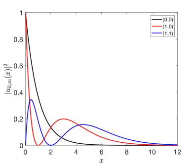
Figure 1: The absolute squared of $u_{k,m}\left(x\right)$ for three sets of $(k,m)$. Note that in the plot $\int\limits_{0}^{\infty}|u_{k,m}\left(x\right)|^{2}dx=1$.

In the presence of the electric field, the Hamiltonian (16) eigenvalues cannot be determined analytically. Consequently, the time-independent non-degenerate perturbation theory is utilized to approximate the required eigenvalues. In this method, it is assumed that the uniform static electric field is sufficiently weak, so that the potential caused by such a field can be regarded as a minor perturbation. In the present study, the eigenvalues of the Hamiltonian (16) are expanded up to the second order of the electric field strength

$$E=E^{(0)}+E^{(1)}F+E^{(2)}F^{2}+\mathcal{O}(F^{3}).$$ (26)

Here $E^{(0)}$, $E^{(1)}$ and $E^{(2)}$ are the zero-, first- and second-order corrections to the eigenvalues, respectively. $E^{(0)}$ coincides to the eigenvalues of hydrogen atom in the Coulomb field given by Eq. (21). $E^{(1)}$ and $E^{(2)}$ are then determined by the time-independent non-degenerate perturbation theory. $E^{(1)}$ is obtained by evaluating

$$E^{(1)} =\langle\psi^{(0)}_{n_{1},n_{2},m}|\dfrac{\xi-\eta}{2}|\psi^{(0)}_{n_{1},n_{2},m}\rangle$$

$$=2\pi A^{2}\int\limits_{0}^{\infty}\int\limits_{0}^{\infty}u^{*}_{n_{1},m}\left(\xi/n\right)u^{*}_{n_{2},m}\left(\eta/n\right)\dfrac{\xi-\eta}{2}u_{n_{1},m}\left(\xi/n\right)u_{n_{2},m}\left(\eta/n\right)|J|d\xi d\eta,$$ (27)

where $u^{*}_{k,m}\left(x\right)=u_{k,m}\left(x\right)$ denotes the complex conjugate of $u_{k,m}\left(x\right)$. Note that in the following, the results of the integrations over $\xi$ and $\eta$ will be automatically multiplied by the factor $2\pi$ because the integration over the azimuthal variable, $\varphi$, always yields the factor $2\pi$.

Substituting the Jacobian given by Eq. (20) into Eq. (3) yields

$$E^{(1)}=E_{1}^{(1)}-E_{2}^{(1)}$$ (28)

with

$$E_{1}^{(1)}=\dfrac{\pi n^{2}A^{2}}{4}\int\limits_{0}^{\infty}\left(\xi/n\right)^{2}u^{2}_{n_{1},m}\left(\xi/n\right)d\left(\xi/n\right)\int\limits_{0}^{\infty}u^{2}_{n_{2},m}\left(\eta/n\right)d\left(\eta/n\right),$$ (29)

$$E_{2}^{(1)}=\dfrac{\pi n^{2}A^{2}}{4}\int\limits_{0}^{\infty}\left(\eta/n\right)^{2}u^{2}_{n_{2},m}\left(\eta/n\right)d\left(\eta/n\right)\int\limits_{0}^{\infty}{u^{2}_{n_{1},m}}\left(\xi/n\right)d\left(\xi/n\right).$$ (30)

Obviously, the integrals $E_{1}^{(1)}$, and $E_{2}^{(1)}$ can be rewritten in an unified form as

$$I_{k,\ell}=\dfrac{\pi n^{2}A^{2}}{4}\int\limits_{0}^{\infty}x^{2}u^{2}_{k,m}(x)dx\int\limits_{0}^{\infty}u^{2}_{\ell,m}(y)dy.$$ (31)

The integral $I_{k,\ell}$ can be evaluated by using the Eq. (12), hence we get

$$E_{1}^{(1)}=I_{n_{1},n_{2}}=\dfrac{1}{4}\left(6n_{1}^{2}+6n_{1}m+6n_{1}+m^{2}+3m+2\right),$$ (32)

$$E_{2}^{(1)}=I_{n_{2},n_{1}}=\dfrac{1}{4}\left(6n_{2}^{2}+6n_{2}m+6n_{2}+m^{2}+3m+2\right).$$ (33)

Plugging Eqs. (32) and (33) to Eq. (28), we obtain

$$E^{(1)}=\dfrac{3}{2}n(n_{1}-n_{2}).$$ (34)

With this first-order correction, the formula describing the eigenvalues’ dependence on the electric field strength is given as

$$E=-\dfrac{1}{2n^{2}}+\dfrac{3}{2}n(n_{1}-n_{2})F+\mathcal{O}(F^{2}).$$ (35)

The Stark effect described by Eq. (35) is called the linear Stark effect since the splitting of the energy levels is

$$\Delta E^{(1)}=\dfrac{3}{2}n(n_{1}-n_{2})F\propto F.$$ (36)

Moreover, substates with identical parabolic quantum numbers, $n_{1}=n_{2}$, do not perceive the applied electric field with the first-order field-induced correction because their distribution of the electrical charge between the $\xi$ and $\eta$ coordinates is symmetric, whereas the linear Stark effect derives from the asymmetric distribution of the electrical charge [35, 34].

The second-order correction to the eigenvalues can be computed as follows,

$$E^{(2)}=\langle\psi^{(0)}_{n_{1},n_{2},m}|\dfrac{\xi-\eta}{2}|\psi^{(1)}_{n_{1},n_{2},m}\rangle$$ (37)

where $|\psi^{(1)}_{n_{1},n_{2},m}\rangle$ is the first-order correction to the eigenfunctions which could be found in Ref [50] and reads as

$$\psi^{(1)}_{n_{1},n_{2},m}(\xi,\eta,\varphi)=\dfrac{n^{3}A}{4}\left[\Phi_{n_{1},m}\left(\xi/n\right)u_{n_{2},m}\left(\eta/n\right)-u_{n_{1},m}\left(\xi/n\right)\Phi_{n_{2},m}\left(\eta/n\right)\right]\exp(im\varphi),$$ (38)

in which

$$\Phi_{k,m}(x)=\dfrac{(k+m)(k+m-1)}{2}u_{k-2,m}(x)-(3n-m-3-2n_{1})(k+m)u_{k-1,m}(x)+\\ +3ku_{k,m}(x)-(3n-m+1-2n_{1})(k+1)u_{k+1,m}(x)+\dfrac{(k+1)(k+2)}{2}u_{k+2,m}(x).$$ (39)

Combining Eqs. (22), (39), and (38) again yields

$$E^{(2)}=E_{1}^{(2)}+E_{2}^{(2)},$$ (40)

where the two integrals $E_{1}^{(2)}$ and $E_{2}^{(2)}$ have an unified form as

$$K_{i,j}=\dfrac{\pi n^{7}A^{2}}{16}\left\{\int\limits_{0}^{\infty}x^{2}\Phi_{i,m}\left(x\right)u_{i,m}\left(x\right)dx\int\limits_{0}^{\infty}u_{j,m}\left(y\right)u_{j,m}\left(y\right)dy\right.+\\ \left.-\int\limits_{0}^{\infty}x^{2}u_{i,m}\left(x\right)u_{i,m}\left(x\right)dx\int\limits_{0}^{\infty}\Phi_{j,m}\left(y\right)u_{j,m}\left(y\right)dy\right\}.$$ (41)

Again, the integral $K_{i,j}$ can be evaluated and derived with the help of Eq. (12)

$$K_{i,j}= \dfrac{n^{3}}{16}\left[4i(i^{2}-1)+6i(i+im+m^{2}+m-1)\right.+$$

$$\left.+(m^{2}+3m+2)(3i-3j+2m-3)+18(i^{2}+im+i)(i-j-2n)\right].$$ (42)

Substituting $E^{(2)}_{1}=K_{n_{1},n_{2}}$ and $E^{(2)}_{2}=K_{n_{2},n_{1}}$ into Eq. (40) yields the second-order correction to the eigenvalues as

$$E^{(2)}=-\dfrac{n^{4}}{16}\left[17n^{2}-3(n_{1}-n_{2})^{2}-9m^{2}+19\right].$$ (43)

Consequently, the formula that describes the so-called quadratic Stark effect is obtained

$$E=-\dfrac{1}{2n^{2}}+\dfrac{3n(n_{1}-n_{2})}{2}F-\dfrac{n^{4}}{16}\left[17n^{2}-3(n_{1}-n_{2})^{2}-9m^{2}+19\right]F^{2}+\mathcal{O}(F^{3}).$$ (44)

In contrast to the linear Stark effect, the quadratic Stark effect involves the splitting of energy levels

$$\Delta E^{(2)}=\dfrac{3n(n_{1}-n_{2})}{2}F-\dfrac{n^{4}}{16}\left[17n^{2}-3(n_{1}-n_{2})^{2}-9m^{2}+19\right]F^{2},$$ (45)

exists even when the electrical charge distribution is symmetric, $n_{1}=n_{2}$. This indicates that the substates are always able to detect the presence of the applied electric field, despite its weakness. When the hydrogen atom is exposed to a uniform static electric field, the degeneracy of substates with the same principal quantum number $n$ is completely eliminated [34, 35].

Using the Siegert State (SS) method, we explicitly verify the exactness and applicability of the approximated formula given by the equation (44) using numerical calculations. Thus, we compute the relative deviation specified by

$$\sigma=\left|\dfrac{E_{ana}-E_{num}}{E_{num}}\right|\times 100\%,$$ (46)

where $E_{num}$ and $E_{ana}$ represent the results of numerical and analytical methods, respectively. Figure 2 illustrates explicitly the evaluation for the ground state and the first excited state with three substates of hydrogen induced by a uniform static electric field. For the ground state, it can be observed that in the regime $0\leq F\leq 0.5$ a.u., the results obtained by the approximated formula and numerical calculation are well-matched, and the relative error is close to $0$. The discrepancy between two approaches increases as the electric-field strength increases; however, it is still less than $1\%$ at $F=0.1$ a.u. In Figs.2(c-d), the three substates of the first excited state exhibit the same characteristic. When $F=0.01$ a.u., the $(0,1,0)$ substate has the maximum relative deviation, below $2\%$, while the $(1,0,0)$ substate has the smallest relative error, approximately $0.5\%$.

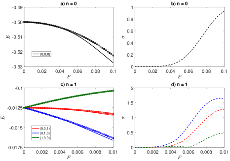
Figure 2: The first column illustrates the dependence of the eigenvalue, $E$, on the external field strength, $F$ for the ground state and the first excited state of the hydrogen atom induced by a static electric field. In the second column, the relative errors between the numerical result obtained by the Siegert State method and the approximated formula are displayed. Note that the solid line represents the numerical results, whereas the squares represent the approximations.

Figure 3 displays the comparison for the excited states with the principle quantum number $n=\{4,6,8,10\}$. In these instances, relative deviations are less than $3.5\%$, which is still an acceptable value.

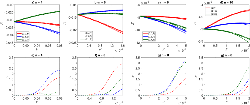
Figure 3: Same as Fig. 2 for a) $n=4$, b) $n=6$, c) $n=8$, and d) $n=10$.

4 Conclusion

In conclusion, we have revisited the quadratic Stark effect of hydrogen for educational purposes. Our method relies on the time-independent non-degenerate perturbation theory and the general integral formula for associated Laguerre polynomials. We have also investigated the applicability interval of the approximated formula describing the quadratic Stark effect of hydrogen using a numerical technique based on the Siegert State method. The comparison demonstrates that when the applied electric field is suitably weak, the approximated formula agrees well with numerical calculations not only for the ground state, but also for highly excited states as well. The approximated formula can therefore be used to predict the eigenvalues of highly excited states in the presence of an exceedingly weak electric field for future high-precision numerical calculations. In addition, we wish to emphasize that, in quantum mechanics, perturbation theory is uncomplicated but never trivial. To address the problem of a stronger electric field, it should be noted that higher-order corrections or improved approaches should be considered; however, these are not our pedagogical objectives. In conclusion, we anticipate that the results of this study will serve as a valuable resource for undergraduates studying quantum mechanics and be readily accessible to them.

References

References

- [1] Chelkowski S, Bandrauk A D and Corkum P B 1990 Physical Review Letters 65 2355
- [2] Lewenstein M, Balcou P, Ivanov M Y, L’huillier A and Corkum P B 1994 Physical Review A 49 2117
- [3] Winterfeldt C, Spielmann C and Gerber G 2008 Reviews of Modern Physics 80 117
- [4] Suran V and Zapesochny I 1975 Sov. Tech. Phys. Lett 1 2
- [5] Rudenko A, De Jesus V, Ergler T, Zrost K, Feuerstein B, Schröter C, Moshammer R and Ullrich J 2007 Physical Review Letters 99 263003
- [6] Bergues B, Kübel M, Johnson N G, Fischer B, Camus N, Betsch K J, Herrwerth O, Senftleben A, Sayler A M, Rathje T et al. 2012 Nature Communications 3 1–6
- [7] Staudte A, Ruiz C, Schöffler M, Schössler S, Zeidler D, Weber T, Meckel M, Villeneuve D, Corkum P, Becker A et al. 2007 Physical Review Letters 99 263002
- [8] Truong T D, Nguyen H H, Le H B, Tran H M, Vy N D, Anh-Tai T D, Pham V N et al. 2022 Computer Physics Communications 276 108372
- [9] Stark J 1913 Nature 92 401–401
- [10] Stark J 1914 Annalen der Physik 348 965–982
- [11] Stark J and Wendt G 1914 Annalen der Physik 348 983–990
- [12] Epstein P S 1916 Annalen der Physik 355 489–520
- [13] Schrödinger E 1926 Annalen der physik 385 437–490
- [14] Epstein P 1926 Physical Review 28 695
- [15] Batishchev P A, Tolstikhin O I and Morishita T 2010 Physical Review A 82 023416
- [16] Pham V, Tolstikhin O and Morishita T 2014 Physical Review A 89 033426
- [17] Ohgoda S, Tolstikhin O I and Morishita T 2017 Physical Review A 95 043417
- [18] Trinh V H, Pham V N, Tolstikhin O I and Morishita T 2015 Physical Review A 91 063410
- [19] Pham V N, Tolstikhin O I and Morishita T 2019 Physical Review A 99 013428
- [20] Wentzel G 1926 Zeitschrift für Physik A Hadrons and Nuclei 38 518–529
- [21] Bekenstein J and Krieger J 1969 Physical Review 188 130
- [22] Alliluev S and Malkin I 1974 Zhurnal Ehksperimental’noj i Teoreticheskoj Fiziki 66 1283–1294
- [23] Lai C 1981 Physics Letters A 83 322–325
- [24] Damburg R J and Kolosov V V 1976 Journal of Physics B: Atomic and Molecular Physics 9 3149
- [25] Damburg R J and Kolosov V V 1978 J. Phys. B: Atom. Molec. Phys. 11 1921–1930
- [26] Damburg R J and Kolosov V V 1979 J. Phys. B: Atom. Molec. Phys. 12 2637–2643
- [27] Damburg R J and Kolosov V V 1981 J. Phys. B. At. Mol. Phys. 14 829–834
- [28] Benassi L, Grecchi V, Harrell E and Simon B 1979 Physical Review Letters 42 704
- [29] Hooker Aand Greene C and Clark W 1997 Physical Review A 55 4609
- [30] Silverstone H 1978 Physical Review A 18 1853
- [31] Alliluev S, Eletsky V, Popov V and Weinberg V 1980 Physics Letters A 78 43–46
- [32] Bolgova I, Ovsyannikov V, Pal’chikov V, Magunov A and von Oppen G 2003 Journal of Experimental and Theoretical Physics 96 1006–1018
- [33] Stodolna A, Rouzée A, Lépine F, Cohen S, Robicheaux F, Gijsbertsen A, Jungmann J, Bordas C and Vrakking M 2013 Physical Review Letters 110 213001
- [34] Landau L D and Lifshitz E M 1958 Quantum mechanics: non-relativistic theory (Pergamon)
- [35] Bethe H and Salpeter E 1957 Quantum mechanics of one- and two-electron atoms (Springer)
- [36] Magnasco V 2006 Elementary methods of molecular quantum mechanics (Elsevier)
- [37] Schwabl F 2007 Quantum mechanics (Springer Science & Business Media)
- [38] Shankar R 2012 Principles of quantum mechanics (Springer Science & Business Media)
- [39] Razavy M 2013 Quantum theory of tunneling (World Scientific)
- [40] Fernández-Menchero L and Summers H 2013 Physical Review A 88 022509
- [41] Griffiths D J and Schroeter D F 2018 Introduction to Quantum Mechanics (Cambridge University Press)
- [42] Rottke H and Welge K 1986 Physical Review A 33 301
- [43] Glab W L, Ng K, Yao D and Nayfeh M H 1985 Physical Review A 31 3677
- [44] Glab W L and Nayfeh M H 1985 Physical Review A 31 530
- [45] Cohen S, Harb M, Ollagnier A, Robicheaux F, Vrakking M, Barillot T, Lepine F and Bordas C 2013 Physical Review Letters 110 183001
- [46] Cohen S, Harb M, Ollagnier A, Robicheaux F, Vrakking M, Barillot T, Lepine F and Bordas C 2016 Physical Review A 94 013414
- [47] Anh-Tai T D, Hoang D T, Truong T D, Nguyen C D, Uyen L N, Dung D H, Vy N D and Pham V N 2021 AIP Advances 11 085310
- [48] Weber H J and Arfken G B 2003 Essential mathematical methods for physicists (Elsevier)
- [49] Anh-Tai T D and Pham V N 2015 Hue University Journal of Science 107 89–97
- [50] Kamenski A and Ovsiannikov V 2000 Journal of Physics B: Atomic, Molecular and Optical Physics 33 491