Pointerformer: Deep Reinforced Multi-Pointer Transformer for the Traveling Salesman Problem

Abstract

Traveling Salesman Problem (TSP), as a classic routing optimization problem originally arising in the domain of transportation and logistics, has become a critical task in broader domains, such as manufacturing and biology. Recently, Deep Reinforcement Learning (DRL) has been increasingly employed to solve TSP due to its high inference efficiency. Nevertheless, most of existing end-to-end DRL algorithms only perform well on small TSP instances and can hardly generalize to large scale because of the drastically soaring memory consumption and computation time along with the enlarging problem scale. In this paper, we propose a novel end-to-end DRL approach, referred to as Pointerformer, based on multi-pointer Transformer. Particularly, Pointerformer adopts both reversible residual network in the encoder and multi-pointer network in the decoder to effectively contain memory consumption of the encoder-decoder architecture. To further improve the performance of TSP solutions, Pointerformer employs both a feature augmentation method to explore the symmetries of TSP at both training and inference stages as well as an enhanced context embedding approach to include more comprehensive context information in the query. Extensive experiments on a randomly generated benchmark and a public benchmark have shown that, while achieving comparative results on most small-scale TSP instances as SOTA DRL approaches do, Pointerformer can also well generalize to large-scale TSPs.

Introduction

The Traveling Salesman Problem (TSP) is a well-known combinatorial optimization problem. It can be stated as follows: given a set of cities/nodes, a salesman departing from one city needs to traverse all other cities exactly once and finally returns to the start city. The objective of TSP is to find the shortest route for the salesman. In addition to its well-recognized theoretical importance as a classic combinatorial optimization problem, TSP also has a wide range of real-world applications, such as drilling of printed circuit boards (Alkaya and Duman 2013), X-Ray crystallography (Bland and Shallcross 1989), warehouse order picking (Madani, Batta, and Karwan 2020), transport routes optimization (Hacizade and Kaya 2018), and many others (Matai, Singh, and Lal 2010).

Due to both of its theoretical and practical importance, TSP has attracted a great number of research efforts in the past decades that attempted to address it using either exact or heuristic algorithms. In fact, the NP-hardness nature of TSP makes it computationally intractable to leverage exact algorithms to find the optimal solutions over a large-scale TSP, since the corresponding computation complexity increases exponentially with respect to the number of nodes. Hence, facing most real-world TSP applications, heuristic algorithms are usually adopted to obtain near-optimal solutions. However, to ensure achieving high-quality solutions, a few heuristic algorithms are designed to further rely on fine-tuned search strategies, which may significantly increase the time complexity for solving large-scale TSP.

Recently, there have been a soaring number of studies trying to solve TSP using either Supervised Learning (SL) or Reinforcement Learning (RL) approaches  (Vinyals, Fortunato, and Jaitly 2015; Nowak et al. 2017; Kool, van Hoof, and Welling 2018; Kwon et al. 2020; Zheng et al. 2021; Fu, Qiu, and Zha 2021a). Compared with SL relying on the optimal solution as the learning labels, which is usually unknown when facing the large-scale TSP, RL yields the advantage since it can be applied to attain near-optimal solutions without requiring the existence of ground truth. Therefore, most recent studies tend to apply the Deep Reinforcement Learning (DRL) approach to solve the large-scale TSP.

Depending on the specific ways to construct solutions, DRL algorithms can be roughly divided into two main categories: search-based DRL (d O Costa et al. 2020; Fu, Qiu, and Zha 2021a) and end-to-end DRL (Kool, van Hoof, and Welling 2018; Kwon et al. 2020; Kim, Park et al. 2021). By incorporating heuristic search operators with learning-based policy, search-based DRL can solve larger-scale TSP instances. However, they usually suffer from two major limitations. The first one lies in the inference efficiency issue, meaning that the search component usually takes a long time to terminate to obtain high quality solutions. Moreover, the obtained solution performance is very sensitive to the selection of search operators which is highly dependent on sophisticated domain knowledge. In contrast, end-to-end DRL algorithms are very efficient in generating solutions and bear much lower dependencies on domain knowledge. Therefore, end-to-end DRL algorithms are more suitable for many emerging TSP application scenarios, such as on-call routing (Ghiani et al. 2003) and ride hailing service (Xu et al. 2018), that require to generate solutions in almost real-time. Nevertheless, most of existing end-to-end DRL algorithms only perform well on small TSP instances (no more than 100 nodes) and cannot generalize to larger instances easily. This is mainly due to the drastically soaring memory consumption and computation time along with the increasing nodes.

In this paper, we propose a novel scalable DRL method based on multi-pointer Transformer, denoted as Pointerformer, aiming to solve TSP in an end-to-end manner. While following the classical encoder-decoder architecture (Vaswani et al. 2017), this new approach adopts reversible residual network (Gomez et al. 2017; Kitaev, Kaiser, and Levskaya 2019) instead of the standard residual network in the encoder to significantly reduce memory consumption. Furthermore, instead of employing the memory-consuming self-attention module as in (Kool, van Hoof, and Welling 2018; Kwon et al. 2020), we propose a multi-pointer network in the decoder to sequentially generate the next node according to a given query. Besides addressing the issues of memory consumption, Pointerformer contains delicate design to further improve the model effectiveness. Particularly, to improve the effectiveness of obtained solutions, Pointerformer employs both a feature augmentation method to explore the symmetries of TSP at both training and inference stages as well as an enhanced context embedding approach to include more comprehensive context information in the query.

To demonstrate the effectiveness of Pointerformer, we conducted extensive experiments on two datasets, including randomly generated instances and widely used public benchmarks. Experimental results have shown that Pointerformer not only achieves comparative results on small-scale TSP instances as SOTA DRL approaches do, but also can generalize to large-scale TSPs. More importantly, while being trained on randomly generated instances, our approach can achieve much better performance on instances with different distributions, indicating a better generalization.

Our main contributions can be summarized as follows.

• We propose an effective end-to-end DRL algorithm without relying on any hand-crafted heuristic operators, which is the first end-to-end DRL approach that can scale to TSP instances with up to 500 nodes to the best of our knowledge.

• Our algorithm applies an auto-regressive decoder with a proposed multi-pointer network to generate solutions sequentially without relying on any search components. Compared with existing search-based DRL algorithms, we can achieve comparable solutions while the inference time is reduced by almost an order of magnitude.

• Besides scalability, we also show via extensive experiments that our approach can generalize well to instances that have varied distributions without re-training.

Related work

Here we highlight a few of the best traditional algorithms for solving TSP, and then focus on presenting the DRL algorithms that are more related to our work.

Traditional TSP algorithms. TSP is one of the most popular combinatorial optimization problems, and numerous algorithms have been proposed for TSP over the past decades. Traditional TSP algorithms can be classified into three categories, i.e., exact algorithms, approximate algorithms and heuristic algorithms. Concorde (Applegate et al. 2007) is one of the fastest exact solvers. It models TSP as a mixed-integer programming problem, and then adopts a branch and cut algorithm (Padberg and Rinaldi 1991) to search the solution. Christofides et al.,  (Christofides 1976) proposed an approximation algorithm, and the approximation ratio of 1.5 is achieved by constructing the minimum spanning tree and the minimum perfect matching of the graph. LKH-3 (Helsgaun 2017) is one of the SOTA heuristics, which uses the $k$-opt operator to search in the solution space, with the guidance of an $\alpha-$measure based on the minimum spanning tree. Among these traditional algorithms, the heuristics are the most widely used algorithms in practice, yet they are still time-consuming and difficult to be extended to other problems.

Besides of these traditional algorithms, there are also works that attempted to utilize the power of machine learning and reinforcement learning techniques. Earlier machine learning approaches include the Hopfield neural network (Hopfield and Tank 1985) and self-organising feature maps (Angeniol, Vaubois, and Le Texier 1988). There are several works like Ant-Q (Gambardella and Dorigo 1995) and Q-ACS (Sun, Tatsumi, and Zhao 2001) that combined reinforcement learning with ant colony algorithm, and Liu and Zeng (Liu and Zeng 2009) used reinforcement learning to improve the mutation of a successful genetic algorithm called EAX-GA (Nagata 2006). It is worth mentioning that a recent work, called VSR-LKH (Zheng et al. 2021), defined a novel Q-value based on reinforcement learning to replace the $\alpha-$value used by the LKH algorithm, and achieved a better performance on TSP.

DL-based TSP algorithms. DL-based TSP algorithms are mainly proposed in recent years, according to the way the solution is generated, they can be classified into two categories: end-to-end methods and search-based methods.

End-to-end methods create a solution from the scratch (Bello et al. 2016; Dai et al. 2017; Kim, Park et al. 2021; Kool, van Hoof, and Welling 2018; Kwon et al. 2020; Nazari et al. 2018; Vinyals, Fortunato, and Jaitly 2015). Vinyals et al.,  (Vinyals, Fortunato, and Jaitly 2015) proposed a Pointer NetWork to solve TSP with SL. Bello et al.,  (Bello et al. 2016) then used RL to train a PtrNet model to minimize the length of solutions. This method achieves better performance and has stronger generalization and scalability. To deal with both static and dynamic information, Nazari (Nazari et al. 2018) improved PtrNet, which is more effective than many traditional methods. Dai et al.,  (Dai et al. 2017) proposed Structure2Vec which encodes partial solutions and predicts the next node. The Q-learning method is used to train the whole policy model. Attention Model in (Kool, van Hoof, and Welling 2018) adopts the Transformer (Vaswani et al. 2017) architecture and the model is trained through the REINFORCE algorithm with a greedy roll-out baseline. It shows the efficiency of Transformer in solving TSP. Then Kwon et al., proposed POMO (Kwon et al. 2020) using REINFORCE algorithm with a shared baseline. It leverages the existence of multiple optimal solutions of a combinatorial optimization problem. Currently, end-to-end methods perform well on TSP instances with nodes less than 100, but due to the complexity of the model and the low sampling efficiency of reinforcement learning, it is hard to extend them to a larger scale.

Search-based methods start from a feasible solution and learn how to constantly improve it (Chen and Tian 2019; d O Costa et al. 2020; Fu, Qiu, and Zha 2021b; Joshi, Laurent, and Bresson 2019; Kool et al. 2022). The improvement is often achieved by integrating with heuristic operators. For instance, Chen et al., proposed NeuRewriter (Chen and Tian 2019), which rewrites local components through region-pick and rule-pick. They trained the model with Advantage Actor-Critic, and the reduced cost per iteration is used as its reward. Two approaches (Joshi, Laurent, and Bresson 2019; Kool et al. 2022) use SL to generate the heat maps of the given graphs, and then employ dynamic programming and beam search to find near-optimal solutions respectively. There is another method using Monte Carlo tree search (MCTS) to improve the solution such as Att-GCRN+MCTS (Fu, Qiu, and Zha 2021b). They first trained a model to generate heat maps for guiding MCTS on small-scale instances by SL, based on which heat maps of larger TSP instances were then constructed by graph sampling, graph converting and heat maps merging. Finally, MCTS is used to search for solutions based on these heat maps. However, performance of such approaches highly depends on the number of iterations or search, which is usually time-consuming hindering their applications in time sensitive tasks.

Problem formulation

While there are many varieties of TSP problems, we focus on the classic two-dimensional Euclidean TSP in this paper. Let $G(V,E)$ denote an undirected full connection graph, where $V=\{v_{i}\mid 1\leq i\leq N\}$ represents all $N$ cities/nodes and $E=\{e_{ij}\mid 1\leq i,j\leq N\}$ is the set of all edges. Let $\mathit{cost}(i,j)$ be the cost of moving from $v_{i}$ to $v_{j}$, which equates the Euclidean distance between $v_{i}$ and $v_{j}$. We further assume $\mathit{depot}\in V$ denoting the depot city, from which the salesman starts the trip and will go back to it in the end. A route is defined as a sequence of cities. A route is feasible iff it starts from and ends at $\mathit{depot}$ while traverses all other cities exactly once. Given a route $\tau$, its total cost, denoted by $L(\tau)$, can be calculated by Eq. (1), where $\tau_{[i]}$ denotes the $i$-th node on $\tau$ and $N=|\tau|$ is the length of $\tau$.

$$L(\tau)=cost(\tau_{[N]},\tau_{[1]})+\sum_{i=1}^{N-1}cost(\tau_{[i]},\tau_{[i+1]}).$$ (1)

A solution $\tau$ of TSP can be generated sequentially by selecting the next node from all nodes that are to be visited until returning to the $\mathit{depot}$. This can be seen as a Markov decision process. The decision of each step can be modeled by a deep neural network parameterized by $\theta$: $\pi_{\theta}(\tau_{[i]}\mid s,\tau[:i))$, where $s$ denotes a TSP instance and $\tau[:i)$ is the partial route on $\tau$ before the $i$-th step. The reward of each step is defined as the negative cost of the newly added edge. For each problem instance $s$, our goal is to maximize the expected cumulative reward defined as follows:

$$J(\theta\mid s)=\mathbb{E}_{\tau\sim p_{\theta}(\tau\mid s)}R(\tau),$$ (2)

where $R(\tau)=-L(\tau)$ and $p_{\theta}(\tau\mid s)=\Pi_{i=1}^{N}\pi_{\theta}(\tau_{[i]}\mid s,\tau[:i))$.

According to the policy gradient theorem (Sutton et al. 2000), we can calculate the derivative of the objective function to update the model using many existing policy gradient algorithms.

$$\nabla_{\theta}J(\theta\mid s)=\mathbb{E}_{p_{\theta}(\tau\mid s)}\left[\nabla_{\theta}\log p_{\theta}(\tau\mid s)R(\tau)\right]$$ (3)

The Pointerformer approach

The proposed Pointerformer is an end-to-end DRL algorithm based on multi-pointer transformer which combines a transformer encoder and an auto-regressive decoder. The general framework of Pointerformer is illustrated in Figure 1.

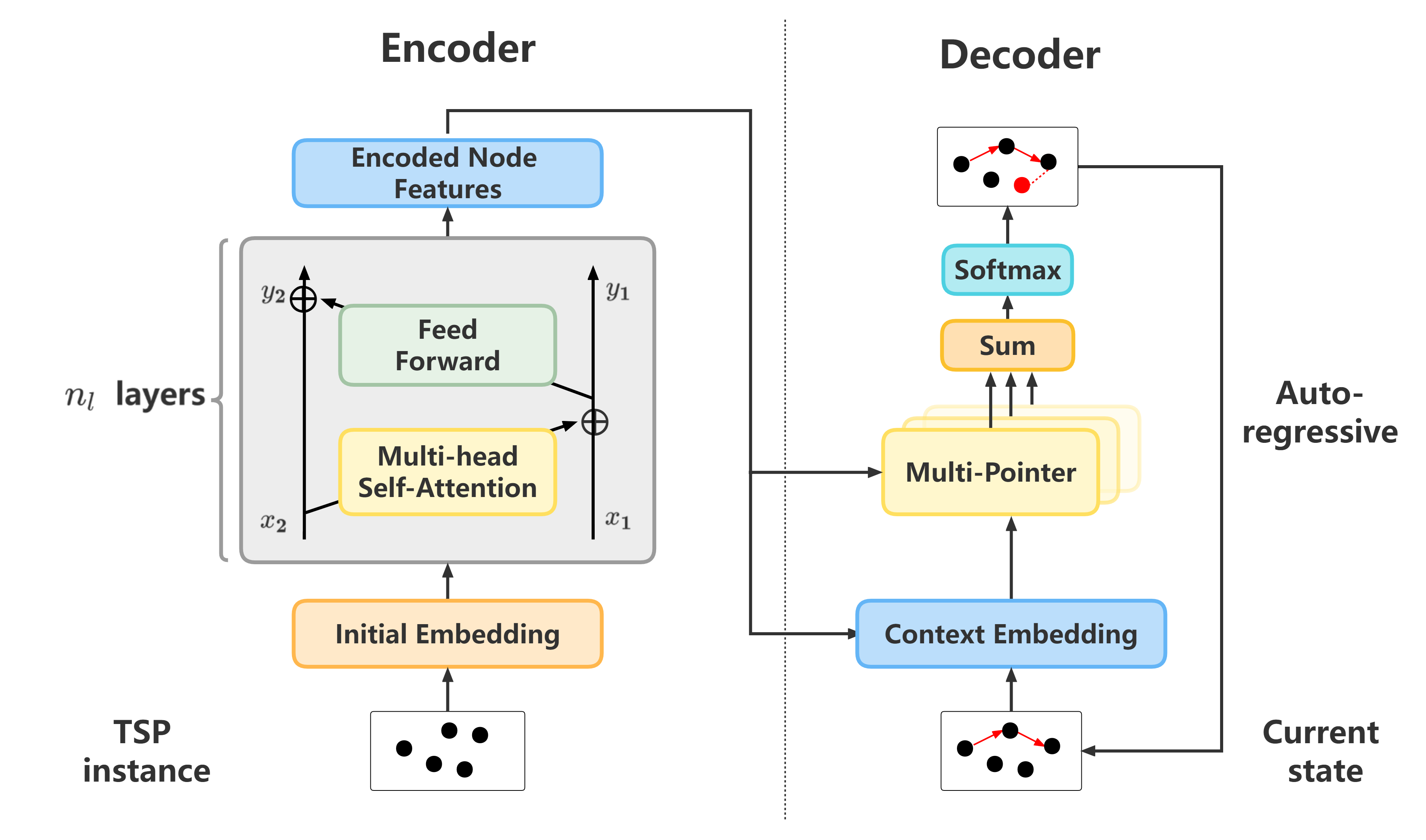
Figure 1: The overall architecture of Pointerformer. First, multiple attention layers are applied to encode the nodes of the input TSP instance. Next, a multi-pointer network is used to sequentially decode the solution by a query composed of an enhanced embedding.

In principle, Pointerformer applies multiple attention layers that consist of multi-head self-attention and feed-forward layers to encode the input nodes for obtaining an embedding of each node. Then, a multi-pointer network with a single head attention is employed to decode sequentially according to a query composed of an enhanced context embedding. Here, the enhanced context embedding contains not only information about the instance itself and nodes that are to be visited, but also information about nodes that have been visited. The solution is generated by choosing a node at each step according to the probability distribution given by the decoder, where all visited nodes are masked so that their probability is 0. Finally, the proposed Pointerformer is trained with a modified REINFORCE algorithm, which is based on a shared baseline for policy gradients while unifying the mean and variance of a batch of instances. In the following subsections, we describe the key components of Pointerformer.

Reversible residual network based encoder

The encoder is an important ingredient for the Pointerformer architecture. As we mentioned before, the resource consumed by the origin Transformer (Vaswani et al. 2017) increases dramatically as the length of the input sequence increases, which equates the number of nodes in TSP. Therefore, we adopt a Transformer without positional encoding but including a reversible residual network, in order to scale to large TSP instances. To our knowledge, the reversible residual network has not been introduced into the DRL approaches of combinatorial optimization problems before.

In the classic two-dimensional Euclidean TSP setting, each node is denoted by its coordinates $(x,y)$ and nothing else. To obtain a robust embedding for each node, we propose a feature augmentation mechanism such that each node is denoted by $(x,y,\eta)$, where $\eta=atanh\frac{y}{x}$. Furthermore, inspired by the data augmentation in POMO (Kwon et al. 2020) that generates 8 equivalent instances of each instance by flipping and rotating its underlying graph, we finally use them on the defined feature to obtain 24 features for each node. These features will be input of the initial embedding layer.

After the initial embedding layer, nodes will go through the encoder with multiple residual layers, each of which is constituted by a multi-head self-attention ($\mathbf{MHA}$) sub-layer and a feed-forward ($\mathbf{FF}$) sub-layer. Here, we employ the reversible residual network (Gomez et al. 2017; Kitaev, Kaiser, and Levskaya 2019) to save memory consumption. Different from residual networks where activation values of all residual layers need to be stored in order to calculate the derivations during back-propagation, in reversible residual networks, $\mathbf{MHA}$ and $\mathbf{FF}$ maintain a pair of input and output embedding features $(X_{1},X_{2})$ and $(Y_{1},Y_{2})$ so that derivations can be calculated directly. Below we illustrate the details in Eq. (4) and (5):

$$Y_{1} =X_{1}+\mathbf{MHA}(X_{2}),$$ (4)

$$Y_{2} =X_{2}+\mathbf{FF}(Y_{1}).$$

Obviously, the input embedding features $(X_{1},X_{2})$ can be calculated from the output embeddings $(Y_{1},Y_{2})$ easily during back-propagation:

$$X_{2} =Y_{2}-\mathbf{FF}(Y_{1}),$$ (5)

$$X_{1} =Y_{1}-\mathbf{MHA}(X_{2}).$$

Note that the deeper of the residual network, the more memory the reversible residual network can save. In our work, we apply $\mathbf{MHA}$ and $\mathbf{FF}$ of six layers, we can observe dramatic reduction of memory consumption without affecting performance.

Multi-pointer network based decoder

The decoder is an auto-regressive process that is to sequentially generate a feasible route for each TSP instance. A context embedding is used to represent the current state, and is used as a query to interact with embeddings of nodes that are to be selected. The context embedding is updated constantly as more nodes are selected until a feasible route is obtained. The auto-regressive decoder is generally very fast but memory-consuming, mainly due to the attention module used in the query. To alleviate this, we improve our decoder by integrating the following distinguishing features.

Enhanced Context Embedding. Recall that a route $\tau$ of TSP is composed of a sequence of nodes on it. We propose an effective and enhanced context embedding that contains the following information $h_{\tau_{[1]}},h_{\tau_{[t]}},h_{g}$, and $h_{\tau}$, where $t=|\tau|$ is used to denote the length of $\tau$:

• $h_{\tau_{[1]}}$ embedding of the first node on $\tau$: A static information that is the embedding of $\mathit{depot}$;

• $h_{\tau_{[t]}}$ embedding of the last node on $\tau$: A dynamic information that is updated according to the current route;

• $h_{g}$ graph embedding: To encode the whole TSP instance, which is the summation of embeddings of all nodes in the instance: $h_{g}=\sum_{i=1}^{N}h^{enc}_{i}$, where $h^{enc}_{i}$ is the embedding of the $i-$th node obtained by the encoder;

• $h_{\tau}$ embedding of $\tau$: To encode the current partial route, which is the summation of embeddings of all nodes on $\tau$ $h_{\tau}=\sum_{i=1}^{t}h_{\tau_{[i]}}^{enc}$.

The enhanced context embedding is used as a query $q_{t}$, which is computed by $q_{t}=\frac{1}{N}(h_{g}+h_{\tau})+h_{\tau_{[t-1]}}+h_{\tau_{[1]}}$. Since the graph embedding is able to reflect different graph structures while information about $\mathit{depot}$ and the last visited node is crucial for selecting future nodes, we include such information to guide the decoder similar as in the previous DRL algorithms (Kool, van Hoof, and Welling 2018; Kwon et al. 2020). Additionally, we also utilize $h_{\tau}$ in our decoder which is ignored in previous solutions. The motivation is that even with the same first and last nodes, two routes may cause different distributions over nodes that are to be visited. As shown in our experiments, such information is crucial, particularly for instances from practical applications. Notice that we normalize the graph embedding and the current partial route embedding by dividing the total number of nodes $N$.

A Multi-pointer Network. At each step, the above enhanced context embedding is used to interact with all nodes that are to be visited to output a probability distribution over them. We devise a multi-pointer network to better utilize the context embedding. More specifically, we linearly project the queries $q_{t}$ and keys $k_{j}$ (embedding of the $j-$th node given by the encoder) to $d_{k}$ dimensions by using $H$ different linear projections for each of them. For each projection, we are able to obtain an interaction between the query and node $j$ via a dot operator and normalization by $\sqrt{d_{k}}$. The final interaction is simply evaluated by an average operator over all $H$ interactions, namely, $\mathit{PN}=\frac{1}{H}\sum_{h=0}^{H}{\frac{{(\mathbf{q}_{t}W_{h}^{q}})^{T}(\mathbf{k}_{j}W_{h}^{k})}{\sqrt{d_{\mathrm{k}}}}}.$

We further minus $\mathit{PN}$ by the cost between the last node $i$ of the partial route and node $j$ to obtain the interaction score between $i$ and $j$: $score_{ij}=\mathit{PN}-\mathit{cost}(i,j)$. By doing so, we encourage the approach to start from a good policy that is always selecting the nearest node as the next one to visit. Comparing to starting from a random policy, this will accelerate our training procedure considerably.

Similar to (Bello et al. 2016), the probability is obtained by Eq. (6), where we clip the score with $\mathit{tanh}$ and mask all visited nodes. Here, $C$ is a coefficient that controls the range of values. The larger $C$ is, the smaller of the entropy, hence can be seen as a parameter to control the trade-off between exploitation and exploration during training. We will show via ablation experiments that the value of $C$ has a significant impact on performance.

$$\vspace{-5pt}u_{ij}=\begin{cases}C\cdot\tanh\left(score_{ij}\right)&\text{node $j$ is to be visited}\\ -\infty&\text{ otherwise }\end{cases}$$ (6)

Finally, we are able to compute the output probability vector $p$ using a $\mathit{softmax}$ function.

A modified REINFORCE algorithm

We train our Pointerformer model by using the REINFORCE algorithm (Williams 1992), whose baseline applies diverse greedy roll-outs of all instances for policy gradient. Inspired by POMO (Kwon et al. 2020), our decoder also starts from $N$ different nodes for each TSP instance with $N$ nodes. By taking each node as the depot, for each TSP instance $i$, we can sample $N$ feasible routes $\tau_{i}=\left\{\tau_{i}^{1},\tau_{i}^{2},\ldots,\tau_{i}^{N}\right\}$ by Monte Carlo sampling method. Therefore, given a batch containing $B$ TSP instances, we can obtain $B\times N$ routes, which can be used to train our policy according to Eq. (3). However, directly applying REINFORCE will cause the algorithm hard to converge because of high variance of costs among different instances. In order to alleviate such a problem, we further use a variance-consistent normalization mechanism before training, which can increase the speed of convergence while also stabilizes the training. More details can be found in Eq. (7), where $\mu(\tau_{i})$ and $\sigma(\tau_{i})$ are the mean and variance of the $N$ trajectories of instance $i$, respectively. One can easily observe that $\frac{R\left(\tau^{j}_{i}\right)-\mu(\tau_{i})}{\sigma(\tau_{i})}$ is an unbiased estimation of the TSP objective function, which eliminates the effect of different rewards among different instances.

$$\nabla_{\theta}J(\theta) \approx\frac{1}{B\times N}\sum_{i=1}^{B}\sum_{j=1}^{N}\left(\frac{R\left(\tau^{j}_{i}\right)-\mu(\tau_{i})}{\sigma(\tau_{i})}\right)\nabla_{\theta}\log p_{\theta}\left(\tau^{j}_{i}\mid s\right),$$ (7)

$$\mu(\tau_{i}) =\frac{1}{N}\sum_{j=1}^{N}R\left(\tau_{i}^{j}\right),$$

$$\sigma(\tau_{i}) =\frac{1}{N}\sum_{j=1}^{N}\left(R\left(\tau_{i}^{j}\right)-\mu(\tau_{i})\right)^{2}.$$

Experiment

To evaluate the efficiency of Pointerformer, we compare its performance with SOTA DRL approaches. We train and test Pointerformer on randomly generated instances, and verified its generalization on a public benchmark.

Benchmark Instances

• TSP_random: Uniformly sample a certain number of nodes from the unit square of $[0,1]^{2}$. It includes five sets of TSP instances with $N$ = 20, 50, 100, 200, 500. Same as in Att-GCRN+MCTS (Fu, Qiu, and Zha 2021b), for TSP instances with $N\leq 100$, we sample 10,000 instances for each set, while for larger instance with $N\geq 200$, the set size is 128. The same benchmark is also widely adopted to testify existing DRL approaches except that they only consider instances with $N\leq 100$;

• TSPLIB: A well-known TSP library (Reinelt 1991) that contains 100 instances with various nodes distributions. These instances come from practical applications with size ranging from 14 to 85,900. In our experiment, we consider all instances with no more than 1002 nodes.

Baselines

The following SOTA DRL algorithms are considered as our baselines.

End-to-end DRL algorithms:

• AM (Kool, van Hoof, and Welling 2018): A model based on attention layer is trained using the REINFORCE algorithm with a deterministic greedy roll-out baseline. AM can achieve good performance on small-scale TSP instances;

• POMO (Kwon et al. 2020): To reduce the variance of advantage estimation, POMO improves the algorithm in AM such that it generates $N$ trajectories for each instance with $N$ nodes and uses data augmentation to improve the quality of solutions during validation;

• AM+LCP (Kim, Park et al. 2021): It proposes a training paradigm for solving TSP called termed learning collaborative policy. It distinguishes policy seeder and policy reviser, which focus on exploration and exploitation, respectively.

Search-based DRL algorithms:

• DRL+2opt (d O Costa et al. 2020): DRL+2opt guides the search of 2-opt operator through DRL. The combination of reinforcement learning and heuristic search operator constantly improve solutions to achieve good results.

• Att-GCN+MCTS (Fu, Qiu, and Zha 2021a): It trains a model to generate heat maps for guiding MCTS on small-scale instances by supervised learning, based on which heat maps of larger instances are then constructed by graph sampling, graph converting and heat maps merging. Finally, MCTS is used to search for solutions based on the heat maps.

Hyper-parameters

In our experiments, we only use instances from TSP_random to train various models corresponding to instances with different nodes. During each training epoch, 100,000 instances are randomly sampled. To train models for instances of size $N\leq 200$, we use a single GPU V100 (16G) with batch size $B=64$, while for other cases the models are trained on four GPUs V100 (32G) with batch size $B=32$. Adam is used as the optimizer for all models with a learning rate $\eta=10^{-4}$ and a weight decay $\omega=10^{-6}$. We use 6 layers in the encoder ($n_{t}=6$) and let $d_{k}=128$ and $H=8$ of multi-pointer in the decoder. The number of heads is 8 in the $\mathbf{MHA}$ layer. When evaluating on TSP_random, the batch size $B$ is 128 for instances with $N\leq 200$, while $B=64$ for other cases. Our algorithm is implemented based on PyTorch (Paszke et al. 2019) and the trained models and the related data will be publicly available once the paper is accepted .

Experimental Results

Table 1: Comparison results on instances from TSP_random.

Method	TSP_random20			TSP_random50			TSP_random100			TSP_random200			TSP_random500
	Len	Gap	Time	Len	Gap	Time	Len	Gap	Time	Len	Gap	Time	Len	Gap	Time
		(%)			(%)			(%)			(%)			(%)
OPT	3.83			5.69			7.76			10.72			16.55
AM	3.83	0.06	5.22s	5.72	0.49	12.76m	7.94	23.20	32.72m	-	-	-	-	-	-
POMO	3.83	0.00	36.86s	5.69	0.02	1.15m	7.77	0.16	2.17m	-	-	-	-	-	-
AM+LCP	3.84	0.00	30.00m	5.70	0.02	6.89h	7.81	0.54	11.94h	-	-	-	-	-	-
DRL+2opt	3.83	0.00	3.33h	5.70	0.12	4.62m	7.82	0.78	6.57h	-	-	-	-	-	-
Att-GCN+MCTS	3.83	0.00	1.6m	5.69	0.01	7.90m	7.76	0.04	15m	10.81	0.88	2.5m	16.97	2.54	5.9m
Pointerformer	3.83	0.00	5.82s	5.69	0.02	11.63s	7.77	0.16	52.34s	10.79	0.68	5.54s	17.14	3.56	59.35s

TSP20, TSP50 and TSP100: 10,000 instances; TSP200 and TSP500: 128 instances.

Table 2: Comparison results on practical instances from TSPLIB.

Method	TSPLIB1$\sim$100			TSPLIB101$\sim$500			TSP501$\sim$1002
	Len	Gap	Time	Len	Gap	Time	Len	Gap	Time
		(%)			(%)			(%)
OPT	19454.17			40842.43			62427.71
AM	22283.67	15.36	0.23s	72137.93	78.18	0.86s	140664.29	139.02	5.79s
POMO	19628.67	1.20	1.41s	43652.77	6.99	1.55s	82162.29	26.93	3.49s
DRL+2opt	19916.50	2.43	15.20m	46651.40	13.85	27.92m	82797.71	42.57	1.24h
Pointerformer (Model100)	19728.50	1.33	0.20s	42963.20	5.43	0.46s	75081.43	18.65	5.14s
Pointerformer (Model200)	20135.00	2.91	0.20s	43810.67	8.37	0.46s	73915.57	18.20	5.14s

To show effectiveness of Pointerformer, we first train models with different number of nodes, denoted by Model$N$ with $N=$ 20, 50, 100, 200, and 500, respectively. For training Model$N$, random instances of size $N$ are sampled from TSP_random using parameters as stated in the above section.

We have conducted the experiment on TSP_random and a further study of generalization on TSPLIB, in all of which we observe advantages of Pointerformer over others. For the group of TSP_random benchmark, the results are shown in Table 1, from which we can see that Pointerformer has the best trade-off between efficiency and optimality compared to others. Pointerformer can achieve results of relatively small gaps to the optimal solutions, denoted by OPT and achieved by running the exact algorithm Concorde. More importantly, one easily observes that Pointerformer can scale to TSP instances with up to 500 nodes while other DRL algorithms except Att-GCN+MCTS quickly run out of memory for TSP instances with $N>100$ (indicated by - in Table 1). In Fig. 2, we also compare memory consumption of our model with the SOTA DRL approach POMO trained on instances of different size. One easily observes that along with the enlarging problem size, the memory consumption of POMO increases sharply, while our model increases gradually. Note that since the architecture of POMO is the most similar with ours, so it is more fair to use POMO for comparison of memory consumption when comparing to other DRL models. Comparing to search-based approach, the solutions obtained by Pointerformer may be slightly worse than Att-GCN+MCTS on TSP instances with 500 nodes. However, we can accelerate the computing time by up to 6 times (5.9m to 59.35s). In particular, we can attain a better result on TSP instances with 200 nodes in less time. We shall mention that results of Att-GCN+MCTS are taken directly from (Fu, Qiu, and Zha 2021b), where the search component is implemented in C++ and runs in a CPU with 8 cores in parallel.

To the best of our knowledge, Pointerformer is the first end-to-end DRL algorithm that can scale to TSP instances with more than 100 nodes while still achieve comparable results as search-based DRL approaches, but in shorter time.

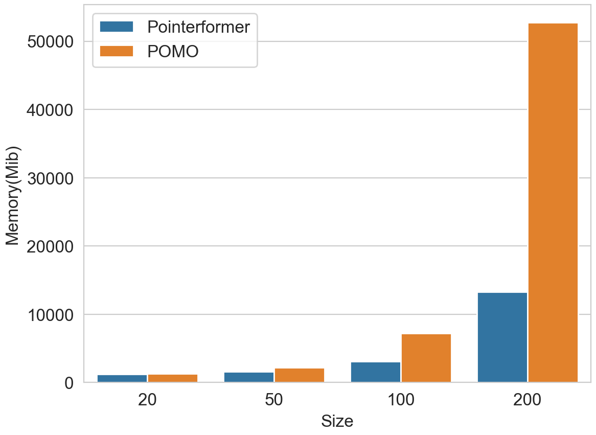
Figure 2: Comparison of memory consumption between Pointerformer and POMO. Along with the enlarging problem size, the memory consumption of POMO increases sharply, while our model increases gradually.

In order to evaluate the generalization of the proposed Pointerformer, we apply Model100 directly to the TSPLIB instances, similar for the baseline algorithms AM, POMO, and DRL+2opt. Note that we do not compare with Att-GCN+MCTS and AM+LCP here, since we have not figured out how to extend Att-GCN+MCTS to non-random setting, while the implementation of AM+LCP is not publicly available. To further verify the importance of scalability, we also apply Model200 to these instances, which are unavailable for the baselines due to lack of scalability. We shall see that Model200 has better generalization comparing to Model100, particularly for large-scale instances. Table 2 summarizes the results of Pointerformer in comparison with the three baselines on instances from TSPLIB, where we classify instances in TSPLIB into three groups according to their sizes, i.e., TSPLIB1$\sim$100, TSPLIB101$\sim$500, and TSPLIB501$\sim$1002. From the results, we can see that POMO performs the best on instances with no more than 100 nodes and the second best on instances between 101 to 500 nodes. While Pointerformer (Model100) performs the best on instances between 101 to 500 nodes and the second best on the other two groups. One notices that most instances of second group are around 100 nodes, so Pointerformer (Model100) has the best performance and POMO has the second best performance for them. Pointerformer (Model200) and Pointerformer (Model100) perform the best and the second best on instances with more than 500 nodes, indicating that our model generalizes best to large-scale instances.

Due to space limit, we only show partial results in the paper. We shall refer interested readers to the appendix for a complete list of our experiment results.

Ablation experiments

In this section, we present some ablation experiment results that explain some important choices of our approach.

Importance of different components of Pointerformer To assess the influence of some key components to the performance of Pointerformer, we carry out an additional ablation study to compare Pointerformer and its four variants on instances from TSP_random with 200 nodes (TSP_random200). The results are summarized in Table 3. The first variant only uses the coordinates of each node as inputs without any feature augmentation (denoted by w.o. feature augmentation in the table). The second variant removes the embedding of the current partial route from the context embedding (denoted by w.o. enhanced context embedding).

Table 3: Ablations of three key elements of Pointerformer on TSP_random200.

Algorithm	Len	Gap
Pointerformer	10.793	0.68%
w.o. feature augmentation	10.813	0.87%
w.o. enhanced context embedding	11.013	2.73%
w.o. multi-pointer network	10.797	0.72%

And the third variant does not use the multi-pointer networks, denoted by w.o. multi-pointer network. From Table 3, it is clear that Pointerformer achieves the best performance comparing to all the variants, which indicates all components play positive roles to our algorithm. Furthermore, we apply these models directly test the instances from TSPLIB and provide their comparisons in Figure 3. Pointerformer with all components outperforms the three variants, indicating that these components are also important for the generalization of Pointerformer.

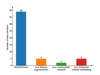
Figure 3: Ablations of three key elements of Pointerformer on TSP_random200.

How $C$ affects the performance As we mentioned before, the value of $C$ in Eq. (6) affects the entropy of distributions over nodes that are to be visited, which consequently has a big impact on the trade-off between exploitation and exploration. As shown in Figure 4, once $C$ is too small ($\leq 10$ in our experiment on instances from TSP_random with 100 and 200 nodes), namely, it encourages exploitation too much, then the algorithm will quickly fall into a local optima. However, once $C$ is big enough ($\geq 50$), the difference will be negligible and the algorithm will constantly converge to a better policy than the one for $C=10$.

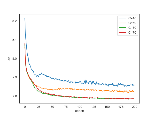
(a)

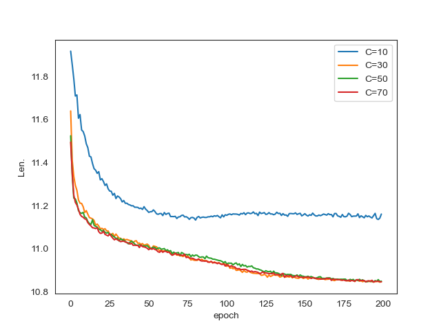
(b)

Figure 4: Comparison of different clipping values.

Conclusion

In this paper, we propose an end-to-end DRL approach called Pointerformer to solve large-scale TSPs. By integrating feature augmentation, reversible residual network, and enhanced context embedding with the well-known Transformer architecture, Pointerformer can achieve comparable results as SOTA algorithms do but using less resources (time or memory). While being memory-efficient, Pointerformer can be scaled to handle TSP instances with 500 nodes, that existing end-to-end DRL approaches could not solve. More importantly, we show via extensive experiments on well-known TSP instances with different distributions that our approach has better generalization. For future work, we will explore how to extend our approach to address the more complicated problem of vehicle routing and other combinatorial optimization problems.

Appendix

More results

We list all the detailed computational results as follows. Furthermore, we also provide four example solutions obtained by our Pointerformer in Figure 5. And one easily observes that even distribution of nodes in TSPLIB instances is different from TSP_random, Pointerformer is able to generalize to different scenarios and makes good routing decisions accordingly.

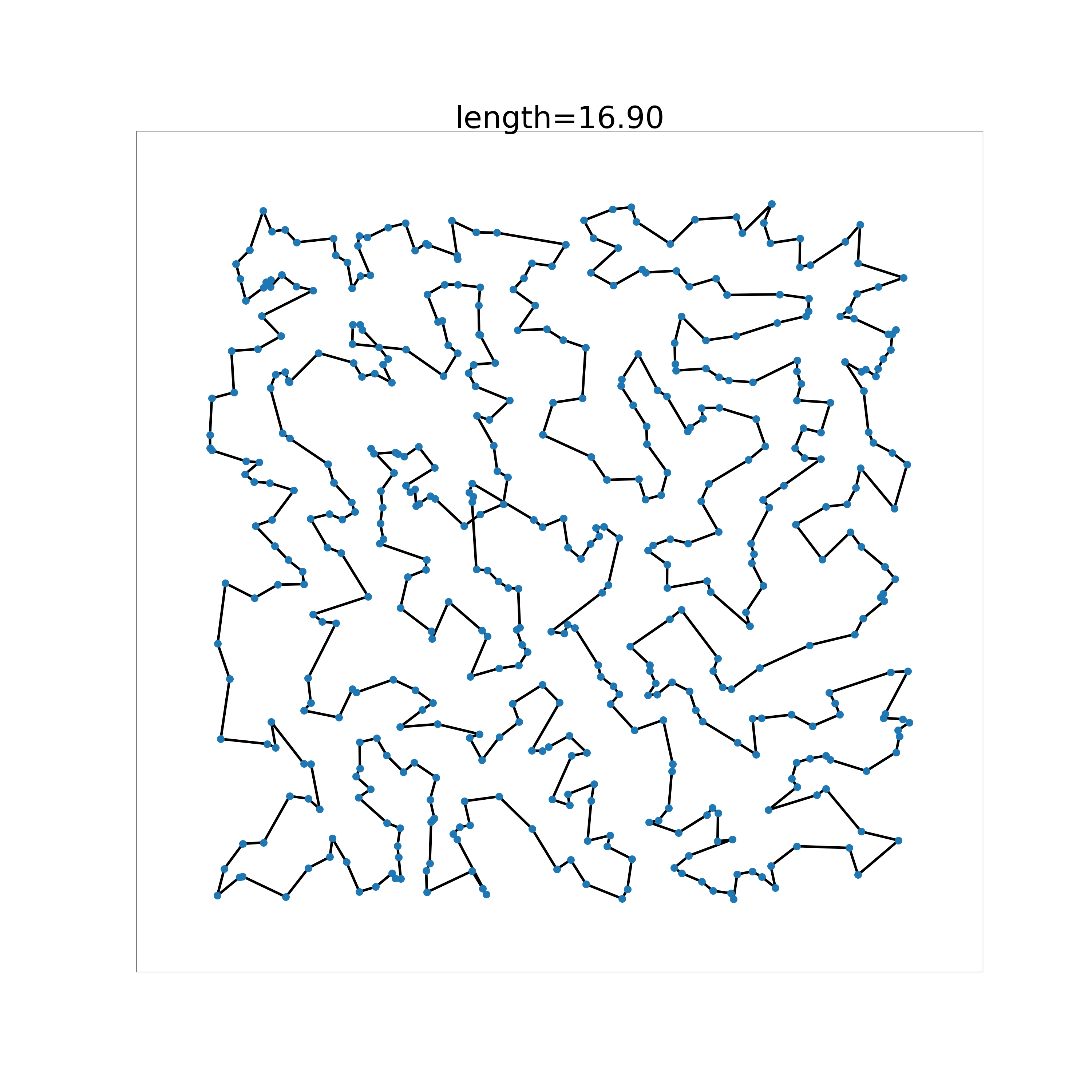
(a)

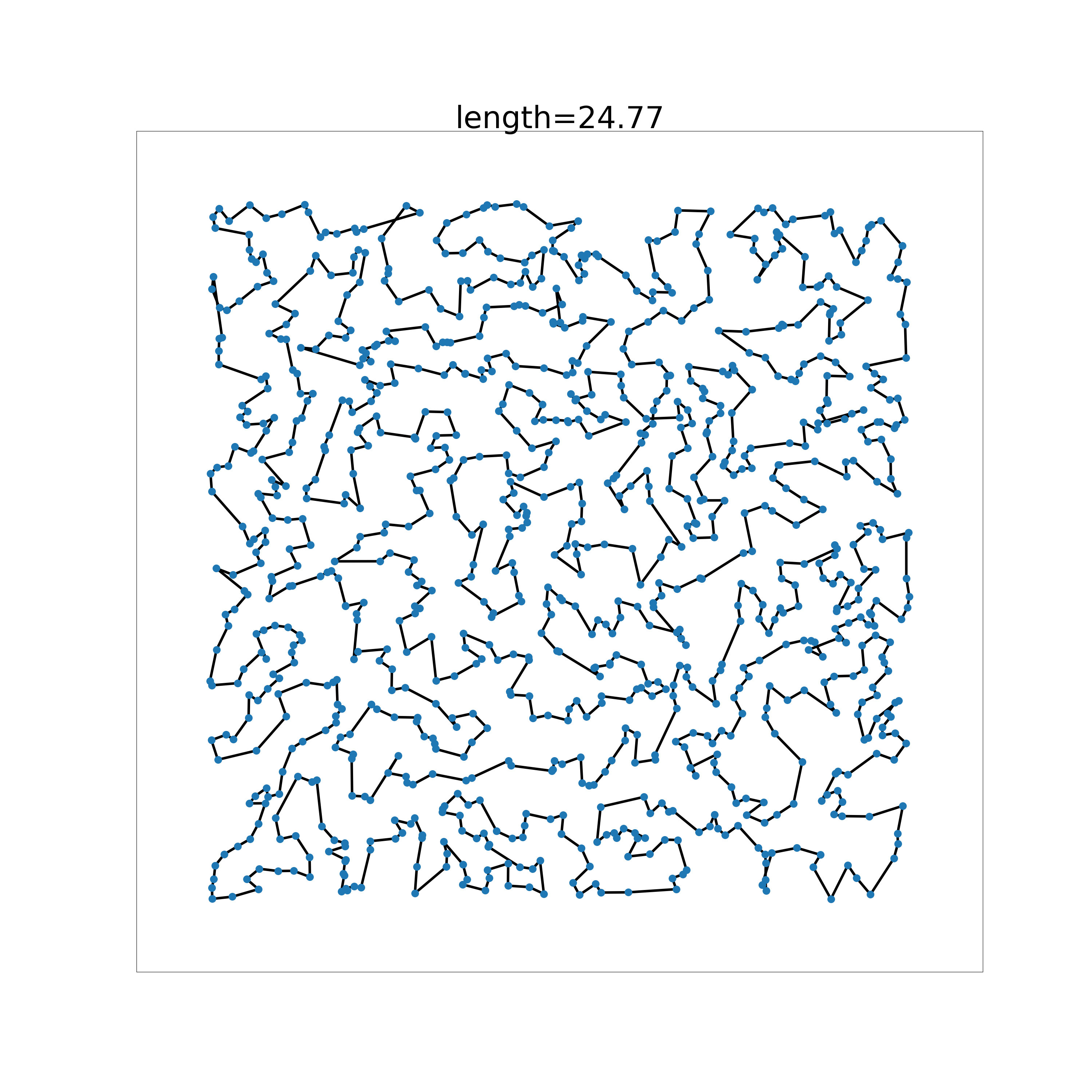
(b)

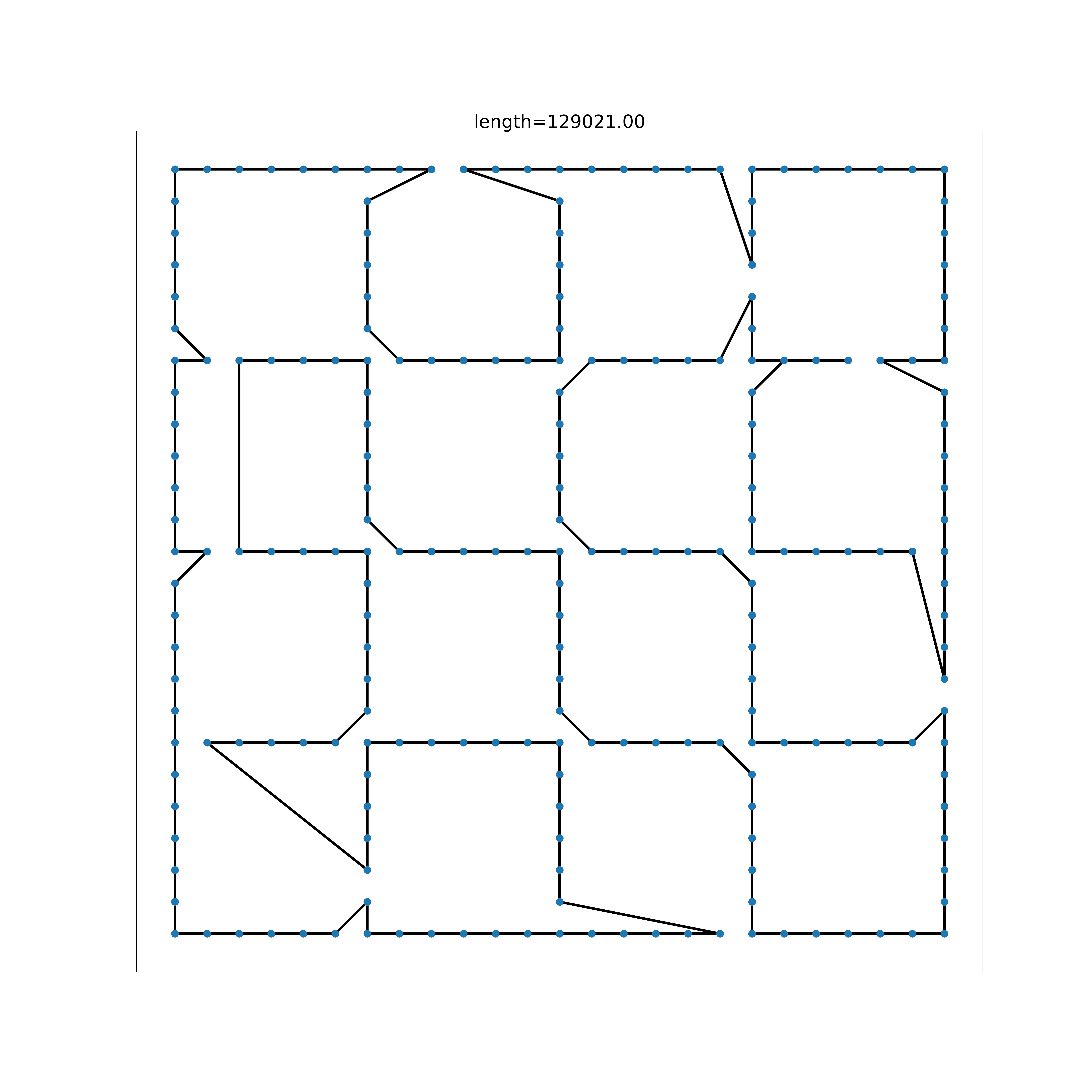
(c)

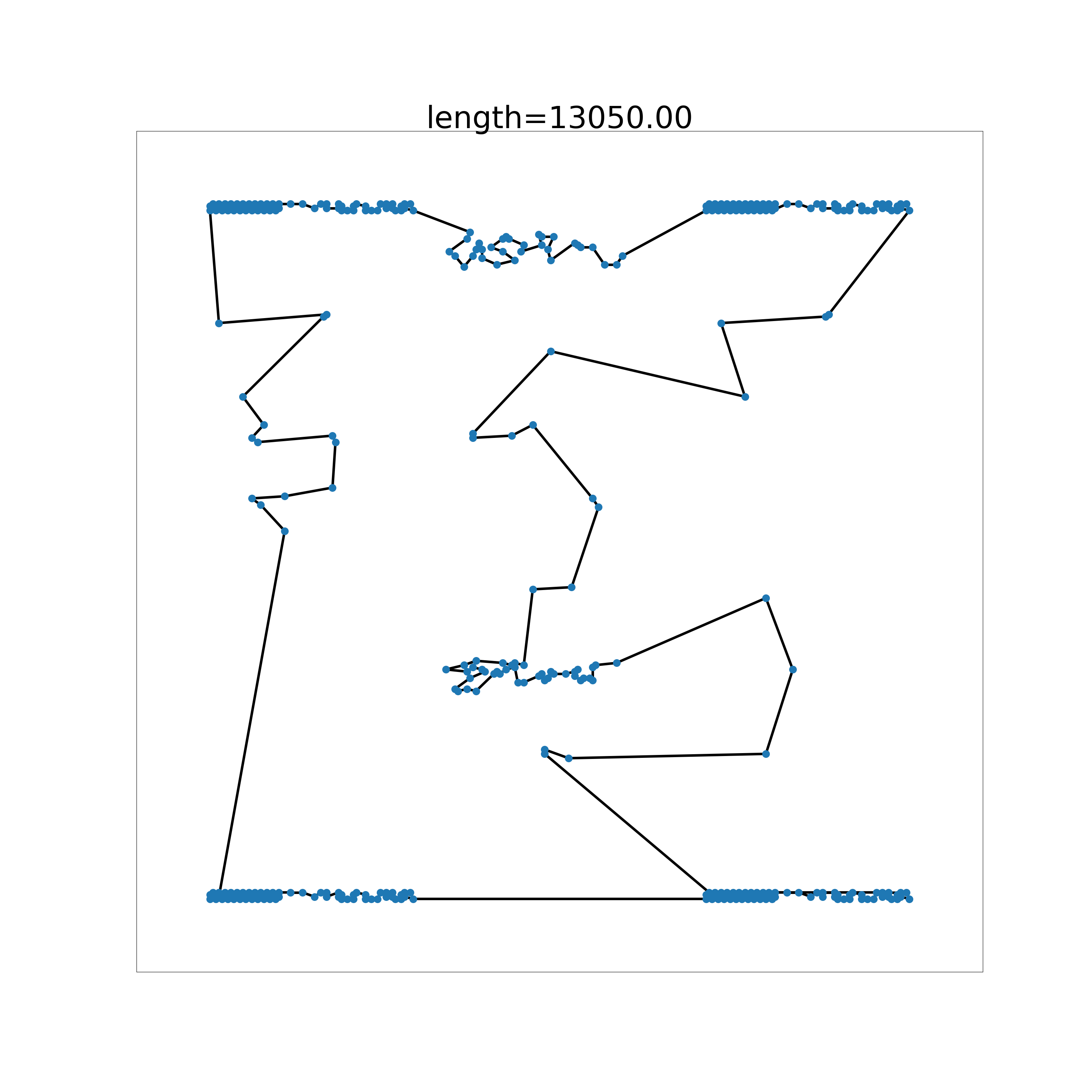
(d)

Figure 5: Example solutions by Pointerformer.

Table 4: Detailed results on practical instances from TSPLIB.

	OPT	Pointerformer (Model100)		Pointerformer (Model200)		POMO		AM		DRL+2opt		AM+LCP
		Len.(Gap)	Time(s)	Len.(Gap)	Time(s)	Len.(Gap)	Time(s)	Len.(Gap)	Time(s)	Len.(Gap)	Time(s)	Len.(Gap)	Time(s)
eil51	426	428(0.47%)	0.20	426(0.00%)	0.20	431(1.17%)	1.33	435(2.11%)	0.86	431(1.17%)	697.24	429(0.73%)	13
berlin52	7542	7542(0.00%)	0.19	7740(2.63%)	0.19	7542(0.00%)	1.38	11336(50.30%)	0.09	7547(0.07%)	703.77	7550(0.10%)	13
st70	675	675(0.00%)	0.17	678(0.44%)	0.17	675(0.00%)	1.43	684(1.33%)	0.12	681(0.89%)	868.52	680(0.74%)	13
eil76	538	538(0.00%)	0.17	541(0.56%)	0.17	538(0.00%)	1.47	550(2.23%)	0.13	549(2.04%)	913.19	547(1.64%)	18
pr76	108159	109117(0.89%)	0.17	111173(2.79%)	0.17	108159(0.00%)	1.48	115300(6.60%)	0.14	109300(1.05%)	873.01	108633(0.44%)	18
rat99	1211	1258(3.88%)	0.19	1274(5.20%)	0.19	1253(3.47%)	1.38	1363(12.55%)	0.20	1252(3.39%)	1007.35	1292(6.67%)	24
kroA100	21282	21452(0.80%)	0.20	21817(2.51%)	0.20	21550(1.26%)	1.41	28464(33.75%)	0.21	22517(5.80%)	959.44	21910(2.95%)	26
kroB100	22141	22579(1.98%)	0.27	23029(4.01%)	0.27	22199(0.26%)	1.38	27755(25.36%)	0.21	23515(6.21%)	985.26	22476(1.51%)	26
kroC100	20749	20958(1.01%)	0.20	21755(4.85%)	0.20	21017(1.29%)	1.43	23653(14.00%)	0.20	20856(0.52%)	967.05	21337(2.84%)	26
kroD100	20749	21923(5.66%)	0.19	22546(8.66%)	0.19	21893(5.51%)	1.50	26274(26.63%)	0.21	22045(6.25%)	949.33	21714(1.97%)	26
kroE100	22068	22362(1.33%)	0.19	22694(2.84%)	0.19	22377(1.40%)	1.30	23415(6.10%)	0.21	22352(1.29%)	972.64	22488(1.90%)	26
rd100	7910	7910(0.00%)	0.20	7947(0.47%)	0.20	7910(0.00%)	1.39	8175(3.35%)	0.20	7953(0.54%)	1044.88	22488(1.90%)	26
eil101	629	630(0.16%)	0.19	632(0.48%)	0.19	630(0.16%)	1.30	643(2.23%)	0.21	639(1.59%)	1046.10	645(2.59%)	26
lin105	14379	14774(2.75%)	0.20	15545(8.11%)	0.20	14580(1.40%)	1.37	32024(122.71%)	0.22	16161(12.39%)	1047.25	14934(3.86%)	26
pr107	44303	45307(2.27%)	0.22	45573(2.87%)	0.22	44907(1.36%)	1.42	46763(5.55%)	0.28	51180(15.52%)	1009.91	-(-%)	-
pr124	59030	59076(0.08%)	0.21	59416(0.65%)	0.21	59076(0.08%)	1.52	61323(3.88%)	0.28	59850(1.39%)	1072.35	61294(3.84%)	37
bier127	118282	121047(2.34%)	0.21	130513(10.34%)	0.21	124531(5.28%)	1.41	135357(14.44%)	0.29	124580(5.32%)	1154.38	128832(8.92%)	37
ch130	6110	6116(0.10%)	0.25	6139(0.47%)	0.25	6124(0.23%)	1.44	6331(3.62%)	0.30	6205(1.55%)	1137.89	6145(0.57%)	38
pr136	96772	97718(0.98%)	0.23	97466(0.72%)	0.23	97493(0.75%)	1.39	102347(5.76%)	0.34	99582(2.90%)	1193.28	98285(1.56%)	38
pr144	58537	58634(0.17%)	0.25	58617(0.14%)	0.25	58924(0.66%)	1.43	64399(10.01%)	0.36	60511(3.37%)	1066.46	60571(3.47%)	43
ch150	6528	6562(0.52%)	0.24	6570(0.64%)	0.24	6558(0.46%)	1.52	6839(4.76%)	0.38	6618(1.38%)	1314.38	-(-%)	-
kroA150	26524	27410(3.34%)	0.25	27736(4.57%)	0.25	26734(0.79%)	1.47	31602(19.14%)	0.40	28400(7.07%)	1311.79	27501(3.68%)	44
kroB150	26130	26810(2.60%)	0.24	27235(4.23%)	0.24	26583(1.73%)	1.51	32043(22.63%)	0.39	27828(6.50%)	1245.82	26962(3.18%)	44
pr152	73682	74610(1.26%)	0.23	74791(1.51%)	0.23	74382(0.95%)	1.47	84778(15.06%)	0.39	78632(6.72%)	1169.23	75539(2.52%)	44
u159	42080	42495(0.99%)	0.26	42487(0.97%)	0.26	42510(1.02%)	1.46	45681(8.56%)	0.42	42800(1.71%)	1286.03	46640(10.84%)	45
rat195	2323	2488(7.10%)	0.31	2490(7.19%)	0.31	2549(9.73%)	1.49	2763(18.94%)	0.58	\textbf{2455(5.68%)}	1639.36	2574(10.81%)	57
d198	15780	18290(15.91%)	0.32	23390(48.23%)	0.32	18766(18.92%)	1.39	85221(440.06%)	0.60	20982(32.97%)	1439.20	-(-%)	-
kroA200	29368	30905(5.23%)	0.31	30509(3.89%)	0.31	29939(1.94%)	1.40	38739(31.91%)	0.59	32208(9.67%)	1558.14	31172(6.14%)	86
kroB200	29437	30978(5.23%)	0.31	30578(3.88%)	0.31	30522(3.69%)	1.42	38106(29.45%)	0.62	31422(6.74%)	1549.52	-(-%)	-
ts225	126643	134522(6.22%)	0.35	128755(1.67%)	0.35	136221(7.56%)	1.58	140768(11.15%)	0.71	132677(4.76%)	1622.01	134827(6.46%)	113
tsp225	3916	4269(9.01%)	0.37	4233(8.09%)	0.37	4142(5.77%)	1.54	5249(34.04%)	0.71	4224(7.87%)	1766.53	4487(14.50%)	113
pr226	80369	81593(1.52%)	0.34	82275(2.37%)	0.34	82632(2.82%)	1.51	93144(15.90%)	0.72	90017(12.00%)	1485.56	85262(6.09%)	113
gil262	2378	2425(1.98%)	0.43	2409(1.30%)	0.43	2440(2.61%)	1.56	2696(13.37%)	0.92	2476(4.12%)	1973.80	2508(5.49%)	134
pr264	49135	51494(4.80%)	0.45	52489(6.83%)	0.45	55003(11.94%)	1.59	68677(39.77%)	0.94	66737(35.82%)	1856.47	-(-%)	-
a280	2579	2824(9.50%)	0.51	2724(5.62%)	0.51	2837(10.00%)	1.67	3330(29.12%)	1.03	2808(8.88%)	2007.79	-(-%)	-
pr299	48191	54718(13.54%)	0.54	54407(12.90%)	0.54	53754(11.54%)	1.60	256687(432.65%)	1.16	61145(26.88%)	2159.60	-(-%)	-
lin318	42029	44312(5.43%)	0.62	44117(4.97%)	0.62	45423(8.08%)	1.58	51507(22.55%)	1.29	47456(12.91%)	2236.29	46540(10.72%)	158
rd400	15281	16659(9.02%)	0.99	15848(3.71%)	0.99	17056(11.62%)	1.75	19010(24.40%)	1.93	17010(11.31%)	2804.61	16519(8.10%)	209
f1417	11861	12782(7.76%)	1.05	12860(8.42%)	1.05	13529(14.06%)	1.83	25813(117.63%)	2.09	17655(48.85%)	2623.33	-(-%)	-
pr439	107217	121515(13.34%)	1.18	117302(9.41%)	1.18	122512(14.27%)	1.96	386134(260.14%)	2.39	151400(41.21%)	2796.83	130996(22.18%)	228
pcb442	50778	56432(11.13%)	1.22	53927(6.20%)	1.22	58287(14.79%)	1.84	67828(33.58%)	2.42	59257(16.70%)	2638.25	57051(12.35%)	228
d493	35002	41501(18.57%)	1.56	63287(80.81%)	1.56	50939(45.53%)	2.00	228336(552.35%)	2.92	56627(61.78%)	3050.07	-(-%)	-
u574	36905	43517(17.92%)	2.40	42967(16.43%)	2.40	45356(22.90%)	2.35	75761(105.29%)	3.73	40197(8.92%)	3838.43	-(-%)	-
rat575	6773	7991(17.98%)	2.40	7844(15.81%)	2.40	8322(22.87%)	2.36	10388(53.37%)	3.75	8539(26.07%)	4108.52	-(-%)	-
p654	34643	38463(11.03%)	3.53	39138(12.98%)	3.53	41978(21.17%)	2.91	117482(239.12%)	4.77	55372(59.84%)	3200.09	-(-%)	-
d657	48912	58113(18.81%)	3.61	63151(29.11%)	3.61	64789(32.46%)	2.99	208309(325.89%)	4.85	78444(60.38%)	4102.30	-(-%)	-
u724	41910	50497(20.49%)	4.88	48292(15.23%)	4.88	52849(26.10%)	3.44	79541(89.79%)	5.79	63492(51.50%)	4751.20	-(-%)	-
rat783	8806	10764(22.23%)	6.22	10562(19.94%)	6.22	11242(27.66%)	3.96	15432(75.24%)	6.68	14815(68.24%)	5592.80	-(-%)	-
pr1002	259045	316225(22.07%)	12.91	305455(17.92%)	12.91	350600(35.34%)	6.43	477737(84.42%)	10.97	318725(23.04%)	5674.53	-(-%)	-

References

- Alkaya and Duman (2013) Alkaya, A. F.; and Duman, E. 2013. Application of sequence-dependent traveling salesman problem in printed circuit board assembly. IEEE Transactions on Components, Packaging and Manufacturing Technology, 3(6): 1063–1076.
- Angeniol, Vaubois, and Le Texier (1988) Angeniol, B.; Vaubois, G. D. L. C.; and Le Texier, J.-Y. 1988. Self-organizing feature maps and the travelling salesman problem. Neural Networks, 1(4): 289–293.
- Applegate et al. (2007) Applegate, D. L.; Bixby, R. E.; Chvátal, V.; and Cook, W. J. 2007. The Traveling Salesman Problem: a Computational Study. Princeton Series in Applied Mathematics.
- Bello et al. (2016) Bello, I.; Pham, H.; Le, Q. V.; Norouzi, M.; and Bengio, S. 2016. Neural combinatorial optimization with reinforcement learning. arXiv preprint arXiv:1611.09940.
- Bland and Shallcross (1989) Bland, R. G.; and Shallcross, D. F. 1989. Large travelling salesman problems arising from experiments in X-ray crystallography: A preliminary report on computation. Operations Research Letters, 8(3): 125–128.
- Chen and Tian (2019) Chen, X.; and Tian, Y. 2019. Learning to perform local rewriting for combinatorial optimization. In Proceedings of the 33rd International Conference on Neural Information Processing Systems, 6281–6292.
- Christofides (1976) Christofides, N. 1976. Worst-case analysis of a new heuristic for the travelling salesman problem. Technical report, Carnegie-Mellon Univ Pittsburgh Pa Management Sciences Research Group.
- d O Costa et al. (2020) d O Costa, P. R.; Rhuggenaath, J.; Zhang, Y.; and Akcay, A. 2020. Learning 2-opt Heuristics for the Traveling Salesman Problem via Deep Reinforcement Learning. In Asian Conference on Machine Learning, 465–480. PMLR.
- Dai et al. (2017) Dai, H.; Khalil, E. B.; Zhang, Y.; Dilkina, B.; and Song, L. 2017. Learning Combinatorial Optimization Algorithms over Graphs. Advances in Neural Information Processing Systems, 30: 6348–6358.
- Fu, Qiu, and Zha (2021a) Fu, Z.; Qiu, K.; and Zha, H. 2021a. Generalize a Small Pre-trained Model to Arbitrarily Large TSP Instances. In Thirty-Fifth AAAI Conference on Artificial Intelligence, AAAI 2021, Thirty-Third Conference on Innovative Applications of Artificial Intelligence, IAAI 2021, The Eleventh Symposium on Educational Advances in Artificial Intelligence, EAAI 2021, Virtual Event, February 2-9, 2021, 7474–7482. AAAI Press.
- Fu, Qiu, and Zha (2021b) Fu, Z.-H.; Qiu, K.-B.; and Zha, H. 2021b. Generalize a Small Pre-trained Model to Arbitrarily Large TSP Instances. In Proceedings of the AAAI Conference on Artificial Intelligence, volume 35, 7474–7482.
- Gambardella and Dorigo (1995) Gambardella, L. M.; and Dorigo, M. 1995. Ant-Q: A reinforcement learning approach to the traveling salesman problem. In Machine learning proceedings 1995, 252–260. Elsevier.
- Ghiani et al. (2003) Ghiani, G.; Guerriero, F.; Laporte, G.; and Musmanno, R. 2003. Real-time vehicle routing: Solution concepts, algorithms and parallel computing strategies. European Journal of Operational Research, 151(1): 1–11.
- Gomez et al. (2017) Gomez, A. N.; Ren, M.; Urtasun, R.; and Grosse, R. B. 2017. The reversible residual network: Backpropagation without storing activations. In Proceedings of the 31st International Conference on Neural Information Processing Systems, 2211–2221.
- Hacizade and Kaya (2018) Hacizade, U.; and Kaya, I. 2018. GA Based Traveling Salesman Problem Solution and its Application to Transport Routes Optimization. IFAC-PapersOnLine, 51(30): 620–625.
- Helsgaun (2017) Helsgaun, K. 2017. An extension of the Lin-Kernighan-Helsgaun TSP solver for constrained traveling salesman and vehicle routing problems. Roskilde: Roskilde University.
- Hopfield and Tank (1985) Hopfield, J. J.; and Tank, D. W. 1985. “Neural” computation of decisions in optimization problems. Biological cybernetics, 52(3): 141–152.
- Joshi, Laurent, and Bresson (2019) Joshi, C. K.; Laurent, T.; and Bresson, X. 2019. An efficient graph convolutional network technique for the travelling salesman problem. arXiv preprint arXiv:1906.01227.
- Kim, Park et al. (2021) Kim, M.; Park, J.; et al. 2021. Learning Collaborative Policies to Solve NP-hard Routing Problems. Advances in Neural Information Processing Systems, 34.
- Kitaev, Kaiser, and Levskaya (2019) Kitaev, N.; Kaiser, L.; and Levskaya, A. 2019. Reformer: The Efficient Transformer. In International Conference on Learning Representations.
- Kool et al. (2022) Kool, W.; van Hoof, H.; Gromicho, J.; and Welling, M. 2022. Deep policy dynamic programming for vehicle routing problems. In International Conference on Integration of Constraint Programming, Artificial Intelligence, and Operations Research, 190–213. Springer.
- Kool, van Hoof, and Welling (2018) Kool, W.; van Hoof, H.; and Welling, M. 2018. Attention, Learn to Solve Routing Problems! In International Conference on Learning Representations.
- Kwon et al. (2020) Kwon, Y. D.; Choo, J.; Kim, B.; Yoon, I.; Gwon, Y.; and Min, S. 2020. POMO: Policy optimization with multiple optima for reinforcement learning. Advances in Neural Information Processing Systems, 2020-December.
- Liu and Zeng (2009) Liu, F.; and Zeng, G. 2009. Study of genetic algorithm with reinforcement learning to solve the TSP. Expert Systems with Applications, 36(3): 6995–7001.
- Madani, Batta, and Karwan (2020) Madani, A.; Batta, R.; and Karwan, M. 2020. The balancing traveling salesman problem: application to warehouse order picking. Top.
- Matai, Singh, and Lal (2010) Matai, R.; Singh, S.; and Lal, M. 2010. Traveling Salesman Problem: an Overview of Applications, Formulations, and Solution Approaches. Traveling Salesman Problem, Theory and Applications.
- Nagata (2006) Nagata, Y. 2006. Fast EAX algorithm considering population diversity for traveling salesman problems. In European Conference on Evolutionary Computation in Combinatorial Optimization, 171–182. Springer.
- Nazari et al. (2018) Nazari, M.; Oroojlooy, A.; Takáč, M.; and Snyder, L. V. 2018. Reinforcement learning for solving the vehicle routing problem. In Proceedings of the 32nd International Conference on Neural Information Processing Systems, 9861–9871.
- Nowak et al. (2017) Nowak, A.; Villar, S.; Bandeira, A. S.; and Bruna, J. 2017. A Note on Learning Algorithms for Quadratic Assignment with Graph Neural Networks. ArXiv e-prints, 1706: arXiv:1706.07450.
- Padberg and Rinaldi (1991) Padberg, M.; and Rinaldi, G. 1991. A branch-and-cut algorithm for the resolution of large-scale symmetric traveling salesman problems. SIAM review, 33(1): 60–100.
- Paszke et al. (2019) Paszke, A.; Gross, S.; Massa, F.; Lerer, A.; Bradbury, J.; Chanan, G.; Killeen, T.; Lin, Z.; Gimelshein, N.; Antiga, L.; Desmaison, A.; Kopf, A.; Yang, E.; DeVito, Z.; Raison, M.; Tejani, A.; Chilamkurthy, S.; Steiner, B.; Fang, L.; Bai, J.; and Chintala, S. 2019. PyTorch: An Imperative Style, High-Performance Deep Learning Library. In Advances in Neural Information Processing Systems 32, 8024–8035. Curran Associates, Inc.
- Reinelt (1991) Reinelt, G. 1991. TSPLIB—A traveling salesman problem library. ORSA journal on computing, 3(4): 376–384.
- Sun, Tatsumi, and Zhao (2001) Sun, R.; Tatsumi, S.; and Zhao, G. 2001. Multiagent reinforcement learning method with an improved ant colony system. In 2001 IEEE International Conference on Systems, Man and Cybernetics. e-Systems and e-Man for Cybernetics in Cyberspace (Cat. No. 01CH37236), volume 3, 1612–1617. IEEE.
- Sutton et al. (2000) Sutton, R. S.; McAllester, D. A.; Singh, S. P.; and Mansour, Y. 2000. Policy gradient methods for reinforcement learning with function approximation. In Advances in neural information processing systems, 1057–1063.
- Vaswani et al. (2017) Vaswani, A.; Shazeer, N.; Parmar, N.; Uszkoreit, J.; Jones, L.; Gomez, A. N.; Kaiser, Ł.; and Polosukhin, I. 2017. Attention is all you need. In Advances in neural information processing systems, 5998–6008.
- Vinyals, Fortunato, and Jaitly (2015) Vinyals, O.; Fortunato, M.; and Jaitly, N. 2015. Pointer Networks. In Cortes, C.; Lawrence, N.; Lee, D.; Sugiyama, M.; and Garnett, R., eds., Advances in Neural Information Processing Systems, volume 28. Curran Associates, Inc.
- Williams (1992) Williams, R. J. 1992. Simple Statistical Gradient-Following Algorithms for Connectionist Reinforcement Learning. In Reinforcement Learning, 5–32. Springer.
- Xu et al. (2018) Xu, Z.; Li, Z.; Guan, Q.; Zhang, D.; Li, Q.; Nan, J.; Liu, C.; Bian, W.; and Ye, J. 2018. Large-scale order dispatch in on-demand ride-hailing platforms: A learning and planning approach. Proceedings of the ACM SIGKDD International Conference on Knowledge Discovery and Data Mining, 905–913.
- Zheng et al. (2021) Zheng, J.; He, K.; Zhou, J.; Jin, Y.; and Li, C.-M. 2021. Combining Reinforcement Learning with Lin-Kernighan-Helsgaun Algorithm for the Traveling Salesman Problem. In Proceedings of the AAAI Conference on Artificial Intelligence, volume 35, 12445–12452.