On the Capacity Region of Reconfigurable Intelligent Surface Assisted Symbiotic Radios

Abstract

In this paper, we are interested in reconfigurable intelligent surface (RIS)-assisted symbiotic radio (SR) systems, where an RIS assists a primary transmission by passive beamforming and simultaneously acts as an information transmitter by periodically adjusting its reflecting coefficients. The above modulation scheme innately enables a new multiplicative multiple access channel (M-MAC), where the primary and secondary signals are superposed in a multiplicative and additive manner. To pursue the fundamental performance limits of the M-MAC, we focus on the characterization of the capacity region of such systems. Due to the passive nature of RISs, the transmitted signal of the RIS should satisfy the peak power constraint. Under this constraint at the RIS as well as the average power constraint at the primary transmitter (PTx), we analyze the capacity-achieving distributions of the transmitted signals and characterize the capacity region of the M-MAC. Then, theoretical analysis is performed to reveal insights into the RIS-assisted SR. It is observed that: 1) the capacity region of the M-MAC is strictly convex and larger than that of the conventional TDMA scheme; 2) the secondary transmission can achieve the maximum rate when the PTx transmits the constant envelope signals; 3) and the sum rate can achieve the maximum when the PTx transmits Gaussian signals and the RIS transmits the constant envelope signals. Finally, extensive numerical results are provided to evaluate the performance of the RIS-assisted SR and verify the accuracy of our theoretical analysis.

I Introduction

Wireless communication systems continue to strive for ever higher data rates and more access devices. It is envisioned that the sixth generation (6G) mobile wireless systems will accommodate up to $1$ terabyte per second (Tb/s) peak data rates and more than $10^{7}$ connections per square kilometer [1, 2]. This goal is particularly challenging for wireless communication systems due to the limited power and spectrum [3]. Symbiotic radio (SR) has emerged as a promising technology to overcome the challenges of spectrum scarcity and high power consumption due to its high spectral and energy efficiencies. Specifically, in SR, a passive secondary transmitter (STx) modulates its information bits over the signal emitted from a primary transmitter (PTx) by periodically adjusting its reflecting coefficient [4]. This modulation scheme innately enables the STx to transmit information without additional spectrum and energy, thereby yielding high spectral and energy efficiencies [5]. In return, the secondary transmission provides multipath gain to the primary transmission, thereby yielding mutual benefits between the two transmissions [6]. Due to its mutualistic potential and high spectral and energy efficiencies, SR has attracted extensive attention from both academia and industry [7, 8].

In SR, there are a number of studies on receiver design and resource allocation. Particularly, the mutualistic condition of SR through which the primary and secondary transmissions can benefit each other is analyzed in [6] from the perspective of bit error rate (BER) performance. Various types of detectors and the corresponding BERs are studied in [9]. In [10], the stochastic optimization techniques are used to jointly design the transmit beamforming and the linear detector. In [11] and [12], the constellation learning detector and the iterative detector are designed, respectively, to recover the transmitted signals of STx when the secondary receiver does not know the pilot information of the primary transmission. As for the resource allocation schemes, the beamforming vectors of PTx are designed in [13] and [14] under the infinite-block length and finite-block length scenarios, respectively. The penalty method is used in [15] to design the beamforming matrix at PTx by maximizing the sum rate of primary and secondary transmissions.

However, the performance of both primary and secondary transmissions is limited by the strength of the backscatter link due to the double fading effect. Fortunately, the reconfigurable intelligent surface (RIS) can operate as an STx to enhance the backscatter link by passive beamforming. Specifically, in the RIS-assisted SR system, the RIS transmits information via passive radio technology and simultaneously assists the primary transmission by reconfiguring the wireless environment. The RIS carries information by periodically adjusting its reflecting coefficients, which is an extension of the backscatter modulation [16]. Besides, RIS can carry information by spatial modulation [17, 18] and symbol level precoding [19, 20], which are summarized in [21]. The existing studies on the RIS-assisted SR mainly focus on the joint design of the transmit beamforming at the PTx and the reflecting coefficients at the RIS. Particularly, the transmit power minimization problem is investigated in [16] for RIS-assisted MIMO SR. The BER minimization, transmit power minimization, and secondary transmission rate maximization problems are studied in [22],  [23], and [24] for the RIS-assisted MISO SR, respectively.

Despite the above notable advancements, the fundamental performance limits of the RIS-assisted SR system have not been addressed well due to the following two reasons. On one hand, the primary and secondary signals in SR are superposed in a multiplicative and additive manner, which forms a new multiplicative multiple access channel (M-MAC). However, over the last few decades, most of the studies focus on the additive multiple access channel (MAC) [25]. When facing the M-MAC, the results of the additive MAC can not be applied directly. On the other hand, the RIS is a passive device whose input should satisfy the peak power constraint. Thus, the widely studied channel capacities under the average power constraint are no longer applicable. Nevertheless, there are still some studies on the M-MAC and on the peak power constraint, respectively, which can provide guidance to the capacity characterization of the RIS-assisted SR.

To be specific, in [26], the capacity region of a binary M-MAC without noise has been explored. The capacity region of the M-MAC with noise is characterized under the average power constraints in [27]. It is worth noting that the capacity region for the above two cases indeed is a triangle. Under the peak constraint, the most interesting result is due to Smith [28], which indicates that the capacity-achieving distribution is discrete with a finite number of mass points. In [29], the peak power limited quadrature Gaussian channel is considered, in which the optimal input distribution is supported on a finite number of concentric circles, i.e., discrete amplitude and uniform independent phase. The $n$-dimensional vector Gaussian noise channel is investigated under the peak power constraint in [30], where the optimal input distribution is geometrically characterized by concentric spheres. Meanwhile, there are some studies on the characterization of the capacity region under the peak power constraint over the additive MAC [31, 32], which show that any point on this capacity region can be achieved by the discrete input distributions of finite support. On the other hand, there are a few studies on the capacity characterization of SR. The achievable rate region with given input distributions is derived for SR in [33]. In [34], the upper bound of the achievable rate for the secondary transmission, i.e., Shannon capacity, is used to analyze the ergodic rate and outage probabilities for both primary and secondary transmissions. In [35], the capacity of the secondary transmission subject to peak power constraint is derived, which, however, does not consider the capacity of the primary transmission and the maximum sum rate in SR. In [36], the capacity of RIS-assisted SR is derived under the condition of discrete transmitted constellation points. In [37], the capacity of the primary transmission is derived, while the capacity of the secondary transmission and the sum rate are not considered. In summary, although there are already several works on M-MAC, peak power constraint, and capacity characterization of SR, respectively, when the M-MAC meets the peak power constraint, the optimal joint distributions and the capacity region of the M-MAC in RIS-assisted SR are still unknown. Meanwhile, the interrelationship between the primary and secondary transmissions in RIS-assisted SR has not been addressed well from the perspective of information theory. Thus, the characterization of the capacity region for RIS-assisted SR is very challenging and crucial.

In this paper, we are interested in the characterization of the capacity region of the M-MAC in the RIS-assisted SR system. To pursue the fundamental performance limits, we first determine the optimal reflecting coefficients of the RIS and analyze the capacity-achieving distributions of the transmitted signals under the average power constraint at the PTx and the peak power constraint at the RIS. Then, we derive the maximum achievable rates for both primary and secondary transmissions. Due to the fact that the rate pairs on the M-MAC capacity region boundary involve the discrete distribution and the continuous distribution, we present one general distribution expression that represents both the discrete and continuous distributions simultaneously. To obtain the distribution parameters in the general distribution expression, we maximize the weighted sum rate of the primary and secondary transmissions, and accordingly characterize the capacity region of the RIS-assisted SR. To reveal insights into the RIS-assisted SR system, we investigate two achievable rate pairs and prove that both of them are on the boundary of the capacity region. The theoretical results show that: 1) the capacity region of the M-MAC is strictly convex and larger than the time division multiple access (TDMA) scheme; 2) the primary transmission can achieve the maximum rate when the RIS only assists the primary transmission; 3) the secondary transmission can achieve the maximum rate when the PTx transmits signals with a constant envelope; 4) the capacity-achieving distribution of the secondary signal is geometrically characterized by concentric circles, whose corresponding rate has more than $4.34$ dB power loss at high SNR compared with Shannon capacity due to the peak power constraint; 5) the sum rate of the primary and secondary transmissions can achieve the maximum when the PTx transmits Gaussian signals and the RIS transmits the constant envelope signals; 6) and when the direct link is weak or blocked, the primary and secondary transmissions can transmit the amplitude and the phase of the Gaussian signals, respectively, to achieve the maximum sum rate. Finally, extensive numerical results are presented to evaluate the performance of the RIS-assisted SR. Surprisingly, even though the secondary signal is unknown to the receiver, the primary transmission can still achieve a higher rate than the rate without the RIS. This implies that the secondary transmission is a beneficial composition instead of interference to the primary transmission. In a nutshell, the main contributions of this paper are summarized as follows.

• We characterize the capacity region for the RIS-assisted SR, which involves the M-MAC, the average power constraint at the PTx, and the peak power constraint at the RIS. We derive the optimal reflecting coefficients of the RIS and the optimal input distributions.

• To reveal insights into the RIS-assisted SR system, we investigate two achievable rate pairs on the boundary of the capacity region, and characterize the performance loss caused by the passive nature of RIS in terms of the capacity region.

• Extensive numerical results are provided to evaluate the performance of the RIS-assisted SR and demonstrate the advantage of M-MAC and the mutually beneficial relationship between primary and secondary transmissions.

The rest of the paper is organized as follows. In Section II, we establish the system model and represent the capacity region mathematically for RIS-assisted SR. The maximum achievable rate for the primary and secondary transmissions are developed in Sections III and IV, respectively. The maximum achievable sum rate is characterized in Section V. The theoretical analysis and the performance evaluation are presented in Sections VI and VII, respectively. Finally, the paper is concluded in Section VIII.

The notation used in this paper is listed as follows. The lowercase and boldface lowercase $x$ and $\mathbf{x}$ denote a scalar variable (or constant) and a vector, respectively. $\mathcal{C}\mathcal{N}(\mbox{\boldmath{$\mu$}},\mbox{\boldmath{$\Sigma$}})$ denotes the complex Gaussian distribution with mean $\mu$ and variance $\Sigma$. The notation $\mathbf{x}^{H}$ denotes the conjugate transpose of $\mathbf{x}$. The notation $\mathbb{E}(\cdot)$ denotes the statistical expectation. The notation $\mathrm{diag}(\mathbf{x})$ denotes a diagonal matrix whose diagonal elements are given by the vector $\mathbf{x}$.

II RIS-assisted SR

In this section, we will describe the system model of the RIS-assisted SR system and illustrate the capacity region mathematically for the RIS-assisted SR system.

II-A System Model

The RIS-assisted SR system consists of a single-antenna PTx, a single-antenna cooperative receiver (C-Rx), and an RIS equipped with $K$ reflecting elements. Let $X_{1}$ denote the signal transmitted by PTx. Due to the active nature of PTx, the primary signal should satisfy the average power constraint, i.e., $\mathbb{E}[|X_{1}|^{2}]\leq P$, where $P$ is the maximum average transmitted power of PTx. The RIS transmits signals by periodically adjusting its reflecting coefficients, i.e., $\mbox{\boldmath{$\phi$}}=[\phi_{1},\cdots,\phi_{K}]^{T}$. Due to the passive nature of RIS, its reflecting coefficients satisfy $|\phi_{k}|^{2}\leq 1$ for $k=1,\cdots,K$. Denote $X_{2}$ as the RIS transmitted signal by RIS, which satisfies the peak power constraint, i.e., $|X_{2}|^{2}\leq 1$. According to the modulation scheme in [16], the mapping rule between $\phi$ and $X_{2}$ is described as $\mbox{\boldmath{$\phi$}}=\mbox{\boldmath{$\varphi$}}X_{2}$, where $\mbox{\boldmath{$\varphi$}}=[\varphi_{1},\cdots,\varphi_{K}]^{T}$ is the passive beamforming vector. Note that the functionality of $\varphi$ is the same as the beamforming vector in traditional wireless communication. The main difference between them is that the power of each element in $\varphi$ is less than one due to the passive nature of RIS.

As shown in Fig. 1, denote by $h_{1}$ the channel coefficient from PTx to C-Rx, by $\mathbf{f}=[\tilde{f}_{1},\cdots,\tilde{f}_{K}]^{T}\in\mathbb{C}^{K\times 1}$ the channel coefficient from PTx to RIS, and by $\mathbf{g}^{H}=[g_{1},\cdots,g_{K}]\in\mathbb{C}^{1\times K}$ the channel coefficient from RIS to C-Rx. The received signal $Y$ at the C-Rx is given by

$${Y} =h_{1}X_{1}+\mathbf{g}^{H}\mbox{\boldmath{$\Psi$}}\mathbf{f}X_{1}X_{2}+{Z}$$

$$=h_{1}X_{1}+h_{2}(\mbox{\boldmath{$\varphi$}})X_{1}X_{2}+{Z},$$ (1)

where $h_{2}(\mbox{\boldmath{$\varphi$}})\triangleq\mathbf{g}^{H}\mbox{\boldmath{$\Psi$}}\mathbf{f}$, $\mbox{\boldmath{$\Psi$}}=\mathrm{diag}(\mbox{\boldmath{$\varphi$}})$, and $Z\sim\mathcal{C}\mathcal{N}(0,\sigma^{2})$ is the additive white Gaussian noise at the C-Rx.

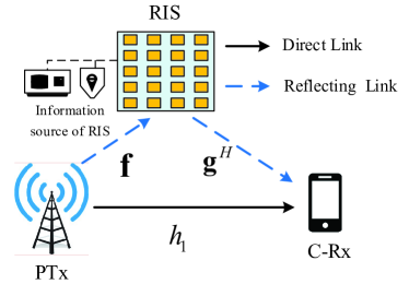
Figure 1: System model.

II-B Capacity Region

Denote by $R_{1}$ and $R_{2}$ the achievable rates of the primary and secondary transmissions, respectively. The capacity region of the M-MAC is the convex hull of the closure of all rate pairs $(R_{1},R_{2})$, which is denoted by $\mathcal{C}_{\mathrm{M-MAC}}$. Following the standard approach in [26], the capacity region of the M-MAC in the RIS-assisted SR is characterized as

$$\mathcal{C}_{\mathrm{M-MAC}}(R_{1},R_{2})=\mathrm{conv}\left(\bigcup_{|\varphi_{k}|^{2}\leq 1}\mathcal{R}(R_{1},R_{2};\mbox{\boldmath{$\varphi$}})\right),$$ (2)

where $\mathrm{conv}(\mathcal{A})$ is the closure of the convex hull of a subset $\mathcal{A}$ and $\mathcal{R}(R_{1},R_{2};\mbox{\boldmath{$\varphi$}})$ is the set of all tuples $(R_{1},R_{2})$ given $\varphi$. Given the distributions of the primary and secondary signals, the tuples $(R_{1},R_{2})$ should satisfy:

$$R_{1} \leq I(X_{1};Y|X_{2}),$$ (3)

$$R_{2} \leq I(X_{2};Y|X_{1}),$$ (4)

$$R_{1}+R_{2} \leq I(X_{1},X_{2};Y).$$ (5)

Note that the capacity region $\mathcal{C}_{\mathrm{M-MAC}}$ goes through all input distributions. In the following, we will present the maximum achievable rates and the maximum sum rate of the primary and secondary transmissions.

III Maximum Achievable Rate of the Primary Transmission

In this section, we will provide the maximum achievable rate of the primary transmission. The maximum achievable rate, also called channel capacity, can be described as

$$C_{1}\triangleq\mathop{\max}\limits_{\mbox{\boldmath{$\varphi$}},f_{1}(X_{1}),f_{2}(X_{2})}I(X_{1};Y|X_{2}),$$ (6)

where $f_{1}(X_{1})$ and $f_{2}(X_{2})$ are the probability density functions (PDFs) of $X_{1}$ and $X_{2}$, respectively. Given $\varphi$, for any distributions $f_{1}(X_{1})$ and $f_{2}(X_{2})$, we have

$$I(X_{1};Y|X_{2}) =\sum_{X_{2}}f_{2}(X_{2})I(X_{1};Y|X_{2}=x_{2})$$

$${\leq}\mathop{\max}\limits_{x_{2}}I(X_{1};Y|X_{2}=x_{2}),$$ (7)

since the average is less than the maximum. That means when the RIS purely assists the primary transmission by passive beamforming, the maximum rate is achievable for the primary transmission. Under the average power constraint, the Gaussian distribution can achieve the maximal entropy over all distributions [26]. Thus, when $X_{1}\sim\mathcal{CN}(0,P)$, the primary transmission can achieve the maximum rate, which is given by

$$C_{1}=\mathop{\max}\limits_{\mbox{\boldmath{$\varphi$}},x_{2}}~{}\log(1+\frac{P|h_{1}+h_{2}(\mbox{\boldmath{$\varphi$}})x_{2}|^{2}}{\sigma^{2}}).$$ (8)

From (8), when $|h_{1}+h_{2}(\mbox{\boldmath{$\varphi$}})x_{2}|^{2}$ is maximized, the primary transmission can achieve the maximum rate, whose solution is $\phi_{k}=\varphi_{k}x_{2}=e^{j(\mathrm{arg}(h_{1})-\mathrm{arg}(\tilde{f}_{k}g_{k}))}$. Accordingly, we have

$$C_{1}=\log(1+\frac{P(|h_{1}|+\sum_{k=1}^{K}|\tilde{f}_{k}||g_{k}|)^{2}}{\sigma^{2}}).$$ (9)

IV Maximum Achievable Rate of the Secondary Transmission

Figure 2: An example of the optimal input distribution with peak power constraint.

In this section, we will provide the maximum achievable rate of the secondary transmission. The maximum achievable rate, i.e., channel capacity, can be described as

$$C_{2}\triangleq\mathop{\max}\limits_{\mbox{\boldmath{$\varphi$}},f_{1}(X_{1}),f_{2}(X_{2})}I(X_{2};Y|X_{1}).$$ (10)

According to [29], the higher transmit power enables a higher achievable rate in the peak power constraint system. Thus, the PTx is required to use its full power to stimulate the secondary transmission. Although the peak power of the PTx can be greater than $P$, the secondary transmission can achieve the maximum rate when the PTx emits a deterministic sinusoidal signal with power $P$. The main reason is that the variation of power will reduce the achievable rate [29]. On the other hand, the stronger the reflecting link is, the higher the achievable rate will be, since the stronger reflecting link will enable a higher signal-to-noise ratio (SNR). Thus, the passive beamforming vector $\varphi$ can be designed by maximizing $|h_{2}(\mbox{\boldmath{$\varphi$}})|^{2}$, whose solution is $\varphi_{k}=e^{-\mathrm{arg}(\tilde{f}_{k}g_{k})}$. Accordingly, the reflecting channel can be written as $h_{2}^{*}=\sum_{k=1}^{K}|\tilde{f}_{k}||g_{k}|$. Thus, the channel capacity of the secondary transmission can be described as:

$$C_{2}=\mathop{\max}\limits_{f_{2}(X_{2})}I(X_{2};\tilde{Y}),$$ (11)

where $\tilde{Y}=\sqrt{P}h_{2}^{*}X_{2}+Z$. Due to physical amplitude constraint, the transmitted signal of the RIS requires to satisfy $|X_{2}|^{2}\leq 1$. Given this constraint, the capacity-achieving distribution is geometrically characterized by concentric circles, i.e., discrete amplitude and uniform independent phase, as shown in Fig. 2 [29]. Denote the amplitude of $X_{2}$ by $r$, whose optimal distribution can be characterized by the following theorem:

Theorem 1 (Characterization of the optimal distribution of the amplitude of $X_{2}$)

Suppose $f_{r^{*}}$ is an optimizer of (11), which is given by

$$f_{r^{*}}(r)=\sum_{\ell=1}^{L}p_{\ell}\delta(r-r_{l}),$$ (12)

with $0\leq r_{l}\leq 1$, $r_{\ell+1}>r_{l}$, $0\leq p_{l}\leq 1$, and $\sum_{\ell=1}^{L}p_{\ell}=1$, where $\delta(\cdot)$ stands for the Dirac-$\delta$ function, $L$ is the number of mass points, $r_{l}$ is the location of the $\ell$-mass point, and $p_{\ell}$ is the corresponding probability of the $\ell$-mass point.

Proof:

Please see [29]. ∎

Note that the number of mass points and the corresponding locations and probabilities can be calculated by maximizing the achievable rate of the secondary transmission, which is given by the following theorem:

Theorem 2 (Capacity of the secondary transmission)

The capacity of the secondary transmission is given by

$$C_{2}=-\int_{0}^{+\infty}\frac{2{r}\kappa({r})}{\sigma^{2}}\log\left(\kappa({r})\right)d{r}-\log(e),$$ (13)

where $\kappa(r)=\sum_{\ell=1}^{L}p_{\ell}\exp\left(-\frac{{r}^{2}+{P}|h_{2}^{*}|^{2}r_{\ell}^{2}}{\sigma^{2}}\right)I_{0}\left(\frac{2{r}\sqrt{P}|h_{2}^{*}|r_{\ell}}{\sigma^{2}}\right)$ and $I_{0}(x)=\frac{1}{2\pi}\int_{-\pi}^{\pi}e^{x\cos\theta}d\theta$.

Proof:

Please see Appendix A. ∎

Compared with the Shannon capacity, the results presented in Theorem 2 provide a more accurate rate bound for the system with peak power constraint. When the SNR is low, the capacity-achieving distribution is geometrically characterized by a unit circle, i.e., the amplitude of $X_{2}$ is equal to $1$, which can be achieved by the symmetric $M$-phase shift-keying examples in practice. With the growth of SNR, the number of the mass points $L$ for the capacity-achieving distribution of the amplitude of $X_{2}$ will increase. This indicates that the number of concentric circles, as shown in Fig. 2, increases with SNR, which corresponds to the quadrature amplitude modulation with peak power constraint in practice.

Theorem 2 presents the maximum achievable rate of the secondary transmission with a complicated expression. Further, the calculations of (12) and (13) are complicated. Here, we provide an upper bound of the capacity of the secondary transmission [38], which has a simplified expression and is given by

$$C_{2}\leq\min\left\{\log\left(1+\sqrt{\frac{\pi P|h_{2}^{*}|^{2}}{\sigma^{2}}}+\frac{P|h_{2}^{*}|^{2}}{e\sigma^{2}}\right)\right.,\left.\log\left(1+\frac{P|h_{2}^{*}|^{2}}{\sigma^{2}}\right)\right\}.$$ (14)

In (14), the first part in the min function represents the McKellips-type bound and the second part represents the Shannon capacity. For low SNR, the capacity of the secondary transmission approaches the Shannon capacity, while the secondary transmission capacity is close to the McKellips-type bound for high SNR. The power loss at high-SNR between the two parts is $10\log_{10}(e)\approx 4.34$ dB. This indicates that if we use the Shannon capacity to approximate the channel capacity under the peak power constraint, we will get a power loss of more than $4.34$ dB at high SNR. Thus, it is essential to analyze the performance of the secondary transmission according to the accurate capacity shown in (13) and the upper bound shown in (14).

V Maximum Achievable Sum Rate

In this section, we will provide the maximum achievable sum rate of the primary and secondary signals. The maximum achievable sum rate can be mathematically described as

$$C_{\mathrm{sum}}\triangleq\mathop{\max}\limits_{\mbox{\boldmath{$\varphi$}},f_{1}(X_{1}),f_{2}(X_{2})}I(X_{1},X_{2};Y).$$ (15)

Since the higher signal power enables a higher achievable rate [25], the passive beamforming vector can be designed as $\varphi_{k}=e^{j(\mathrm{arg}(h_{1})-\mathrm{arg}(\tilde{f}_{k}g_{k}))}$ to enhance the reflecting link and align with the direct link. However, the RIS-assisted SR system involves the M-MAC, the average power constraint, and the peak power constraint, leading to the difficulty in obtaining the optimal joint distribution of $X_{1}$ and $X_{2}$ directly. In fact, on the capacity region boundary, the distributions of the amplitude of $X_{1}$ involve the discrete one and the continuous one, which will be detailedly discussed in Section VI. In what follows, we will present one general distribution expression that can represent the discrete distribution and the continuous distribution simultaneously, based on which we will characterize the capacity region of the RIS-assisted SR.

V-A General Distribution Expressions for Primary and Secondary Signals

To explore the distribution of the amplitude of $X_{1}$, we use the discrete variable distribution to approach the continuous variable distribution. Specifically, we assume that the distribution of the amplitude of $X_{1}$ follows

$${f_{{s^{*}}}}(s)= \mathop{\lim}\limits_{M\rightarrow\infty}\sum_{m=1}^{M}{{q_{m}}}\delta(s-{s_{m}}),$$ (16)

$$s.t.~{}~{}~{}~{} {\mathbb{E}}{\left|{{s_{m}}}\right|^{2}}\leq P,0\leq q_{m}\leq 1,\mathrm{and}\sum_{m=1}^{M}q_{m}=1,$$

where $s$ is the amplitude of $X_{1}$, $M$ is the number of mass points, $s_{m}$ is the location of the $m$-mass point, and $q_{m}$ is the corresponding probability of the $m$-mass point. Meanwhile, the phase of $X_{1}$ follows the uniform independent distribution from $-\pi$ to $\pi$. Note that when $M\rightarrow\infty$, the discrete variable distribution can approach the continuous variable distribution. Even with $M\rightarrow\infty$, the distribution of $s$ in (16) can represent a discrete one since the value of $s_{m}$ can be the same. For example, if $s_{m}=1$ for all $m$, the amplitude of $X_{1}$ is only equal to $1$, yielding a discrete distribution over $s$. Thus, the distribution in (16) can represent a discrete one.

Similarly, the distribution of the amplitude of the secondary signal $X_{2}$ is shown in (12) and the phase of $X_{2}$ follows the uniform independent distribution from $-\pi$ to $\pi$.

V-B Capacity Region Characterization

Since the MAC capacity region is convex, it is well known that the boundary of the capacity region can be characterized by maximizing the function $\mu_{1}R_{1}+\mu_{2}R_{2}$ over all rate pairs in the capacity region [39]. Note that the capacity priorities $(\mu_{1},\mu_{2})$ are nonnegative and satisfy $\mu_{1}+\mu_{2}=1$. For a fixed set $(\mu_{1},\mu_{2})$, the slope of the tangent of one point on the capacity region boundary is defined by the priorities. This implies that the boundary points with different slopes of the capacity region may correspond to different distributions for both primary and secondary transmissions. Furthermore, according to [39], the order of the increasing priority will affect the successive decoding. Specifically, the user with the lower priority will be decoded first. When decoding the primary signal first, the capacity region can be characterized by maximizing $\mu_{1}I(X_{1},Y)+\mu_{2}I(X_{2},Y|X_{1})$, which is given by the following theorem.

Theorem 3

When decoding the primary signal first, the achievable rates for both primary and secondary transmissions can be calculated by

$$I(X_{1};Y) =\sum_{m=1}^{M}q_{m}\int_{0}^{+\infty}\frac{2{r}\bar{\kappa}({r},s_{m})}{\sigma^{2}}\log\left({\bar{\kappa}({r},s_{m})}\right)d{r}-\int_{0}^{+\infty}\!\frac{2{r}\check{\kappa}({r})}{\sigma^{2}}\log\left(\check{\kappa}({r})\right)d{r},$$ (17)

$$I(X_{2};Y|X_{1}) =-\sum_{m=1}^{M}q_{m}\int_{0}^{+\infty}\frac{2{r}\bar{\kappa}({r},s_{m})}{\sigma^{2}}\log\left({\bar{\kappa}({r},s_{m})}\right)d{r}-\log(e),$$ (18)

where $\bar{\kappa}({r},s_{m})\!=\!\sum_{\ell}^{L}p_{\ell}\!\exp\!\left(-\frac{{r}^{2}+|h_{2}|^{2}|s_{m}|^{2}|r_{\ell}|^{2}}{\sigma^{2}}\!\right)\!I_{0}\left(\frac{2{r}|h_{2}||s_{m}||r_{\ell}|}{\sigma^{2}}\right)$, $\check{\kappa}({r})\!=\!\sum_{\ell=1}^{L}\!\frac{p_{\ell}q_{m}}{4\pi^{2}}\!\exp\!\left(\!-\frac{{r}^{2}+|h_{1}|^{2}s_{m}^{2}}{\sigma^{2}}\!\right)$ $\exp\!\left(\!\!\frac{-|h_{2}|^{2}r_{\ell}^{2}s_{m}^{2}}{\sigma^{2}}\!\!\right)\!\!\int_{-\pi}^{\pi}\!\!\int_{-\pi}^{\pi}\!\exp\!\!\left(\!\!\frac{-2|h_{1}||h_{2}|s_{m}^{2}r_{\ell}\cos(\theta_{2})+2{r}\!\sqrt{|h_{1}|^{2}s_{m}^{2}\!+\!|h_{2}|^{2}r_{\ell}^{2}s_{m}^{2}\!+\!2|h_{1}||h_{2}|s_{m}^{2}r_{\ell}\cos(\theta_{2})}\!\cos(\theta_{1}\!+\!\alpha(\theta_{2}))}{\sigma^{2}}\!\!\right)\!\!d\theta_{1}d\theta_{2}$, and $\alpha(\theta_{2})=\arctan(\frac{|h_{2}|s_{m}r_{\ell}\sin(\theta_{2})}{|h_{1}|s_{m}+|h_{2}|s_{m}r_{\ell}\cos(\theta_{2})})$.

Proof:

Please see Appendix B. ∎

When decoding the secondary signal first, the capacity region can be characterized by maximizing $\mu_{1}I(X_{1},Y|X_{2})+\mu_{2}I(X_{2},Y)$, which is given by the following theorem.

Theorem 4

When decoding the secondary signal first, the achievable rates for both primary and secondary transmissions can be calculated by

$$\!\!I(X_{1};Y|X_{2})\!=\!-\sum_{\ell=1}^{L}p_{\ell}\int_{-\pi}^{\pi}\int_{0}^{+\infty}\frac{2{r}\underline{\kappa}({r},r_{\ell},\theta_{2})}{\sigma^{2}}\log\left({\underline{\kappa}({r},r_{\ell},\theta_{2})}\right)d{r}d\theta_{2}-\log(e)$$ (19)

$$\!\!I(X_{2};Y)\!=\!\sum_{\ell=1}^{L}p_{\ell}\int_{-\pi}^{\pi}\!\int_{0}^{+\infty}\!\frac{2{r}\underline{\kappa}({r},r_{\ell},\theta_{2})}{\sigma^{2}}\!\log\left({\underline{\kappa}({r},r_{\ell},\theta_{2})}\right)d{r}d\theta_{2}\!-\!\!\int_{0}^{+\infty}\!\!\frac{2{r}\check{\kappa}({r})}{\sigma^{2}}\!\log\left(\check{\kappa}({r})\right)d{r},$$ (20)

where $\underline{\kappa}({r},r_{\ell},\theta_{2})=\sum_{m=1}^{M}q_{m}\exp\left(-\frac{{r}^{2}+|h_{1}+h_{2}r_{\ell}e^{j\theta_{2}}|^{2}|s_{m}|^{2}}{\sigma^{2}}\right)I_{0}\left(\frac{2{r}|h_{1}+h_{2}r_{\ell}e^{j\theta_{2}}||s_{m}|}{\sigma^{2}}\right)$.

Proof:

Please see Appendix C. ∎

Based on Theorem 3 and Theorem 4, the problems of finding the boundary point on the capacity region associated with priorities can be written as

$$\mathbf{P1}:\;\;\mathop{\max}\limits_{L,M,r_{\ell},s_{m},p_{\ell},q_{m}}\;\; \mu_{1}I(X_{1};Y)+\mu_{2}I(X_{2};Y|X_{1})$$

$$\mathrm{s.t.}~{}~{}~{}~{}~{}~{}\;\; \mathrm{C1}:{f_{{s^{*}}}}(s)=\mathop{\lim}\limits_{M\rightarrow\infty}\sum_{m=1}^{M}{{q_{m}}}\delta(s-{s_{m}}),~{}~{}\mathrm{C}2:f_{r^{*}}(r)=\sum_{\ell=1}^{L}p_{\ell}\delta(r-r_{l}),$$

$$\mathrm{C}3:0\leq r_{l}\leq 1,~{}~{}\mathrm{C}4:r_{\ell+1}>r_{l},~{}~{}\mathrm{C}5:0\leq p_{l}\leq 1,~{}~{}\mathrm{C}6:\sum_{\ell=1}^{L}p_{\ell}=1,$$

$$\mathrm{C}7:{\mathbb{E}}{\left|{{s_{m}}}\right|^{2}}\leq P,~{}~{}\mathrm{C}8:0\leq q_{m}\leq 1,~{}~{}\mathrm{C}9:\sum_{m=1}^{M}q_{m}=1,$$

and

$$\mathbf{P2}:\;\;\mathop{\max}\limits_{L,M,r_{\ell},s_{m},p_{\ell},q_{m}}\;\; \mu_{1}I(X_{1};Y|X_{2})+\mu_{2}I(X_{2};Y)$$

$$\mathrm{s.t.}~{}~{}~{}~{}~{}~{}\;\; \mathrm{C}1-\mathrm{C}9,$$

respectively. By solving the above two optimization problems with the interior-point algorithm, we can characterize the capacity region for the RIS-assisted SR system. From the solved distributions, we can analyze the characteristics and variation of the optimal distributions on the boundary of the capacity region, which will be shown in Section VII.

As aforementioned, the capacity region of RIS-assisted SR can be characterized by solving optimization problems. Although it is difficult to analyze the capacity-achieving distributions for each rate pair on the capacity region boundary, we can still investigate some important corner points on the capacity region to obtain more insights into the RIS-assisted SR, which will be presented in the next section.

VI Theoretical Analysis

In this section, to obtain essential insights, we will investigate two rate pairs on the capacity region boundary for the RIS-assisted SR system. The investigation will be presented in the following two scenarios, i.e., the direct link is present and absent, respectively.

VI-A Direct Link is Present

VI-A1 Rate Pair A on Capacity Region Boundary

Here, we are interested in the possible rate pairs that can achieve the maximum rate of the primary or secondary transmissions while the other can still transmit information. In fact, the primary signal achieves its maximum rate only when the reflecting coefficients of RIS remain unchanged given one channel realization. However, the secondary transmission requires that the RIS periodically adjusts its reflecting coefficients. Hence, the maximum rate is unachievable for the primary transmission when the RIS transmits signals. In contrast, we find that when $|X_{1}|^{2}=P$, the secondary transmission can still achieve its maximum rate, which is shown in the following theorem:

Theorem 5

Given $|X_{1}|^{2}=P$, the secondary transmission can achieve the maximum rate.

Proof:

Given $|X_{1}|^{2}=P$, the mutual information of the secondary transmission can be written as $I(X_{2};Y|X_{1})=H(Y|X_{1})-\log(\pi e\sigma^{2})$. Since adding a constant does not change the differential entropy, we have $H(Y|X_{1})=H(h_{2}X_{1}X_{2}+{Z}|X_{1})$. Let us multiply $h_{2}X_{1}X_{2}+{Z}$ by $\frac{X_{1}^{H}}{|X_{1}|}$, yielding $\frac{X_{1}^{H}}{|X_{1}|}(h_{2}X_{1}X_{2}+Z)=\sqrt{P}h_{2}X_{2}+\tilde{Z}$ with $\tilde{Z}\sim\mathcal{CN}(0,\sigma^{2})$. Since $H(\sqrt{P}h_{2}X_{2}+\tilde{Z})=H(\sqrt{P}h_{2}X_{2}+{Z})$, we can find that given $|X_{1}|^{2}=P$, the mutual information between $X_{2}$ and $Y$ is equal to the result in (13). ∎

The above theorem shows that when the PTx transmits signals with the constant envelope, the secondary transmission can achieve the maximum rate, shown as (13). In fact, according to the chain rule, the primary signal $X_{1}$ needs to be decoded first, i.e., $I(X_{1},X_{2};Y)=I(X_{1};Y)+I(X_{2};Y|X_{1})$. In such a setting, the achievable rates $R_{1}^{\mathrm{A}}=I(X_{1};Y)$ of the primary transmission and $R_{2}^{\mathrm{A}}=I(X_{2};Y|X_{1})$ of the secondary transmission can be calculated by using the Theorem 3 where $s_{m}=1,\forall m$, and $r_{\ell}$ and $p_{\ell}$ are obtained by maximizing the secondary transmission rate.

VI-A2 Rate Pair B on Capacity Region Boundary

By defining ${X}=h_{1}X_{1}+h_{2}X_{1}X_{2}$, the received signal at the C-Rx is given by $Y=X+Z$, where ${X}$ can be treated as the virtual transmitted signal. Due to the constraints of $X_{1}$ and $X_{2}$, the virtual signal ${X}$ satisfies the average power constraint, which is given by

$$\mathbb{E}[|{X}|^{2}]\overset{(a)}{=}|h_{1}|^{2}\mathbb{E}[|X_{1}|^{2}]+|h_{2}|^{2}\mathbb{E}[|X_{1}|^{2}]\mathbb{E}[|X_{2}|^{2}]+2|h_{1}h_{2}|\mathbb{E}[|X_{1}|^{2}]\mathbb{E}[\textit{Re}(X_{2})],$$ (23)

where $(a)$ holds due to the alignment between the reflecting link and the direct link. According to [26], we know that when ${X}$ follows Gaussian distribution, the entropy can achieve the maximum over all distributions. Thus, to maximize the sum rate, we aim to design the scheme that ${X}$ follows Gaussian distribution with higher average power.

From (23), it can be found that when $X_{2}=1$, the average power of ${X}$ is the maximum, and the virtual signal ${X}$ follows Gaussian distribution. In this case, the RIS does not transmit information, and the PTx transmits the Gaussian signal with the maximum achievable rate. When the RIS transmits signals, we have $\mathbb{E}[\textit{Re}(X_{2})]\leqslant 1$ due to the peak power constraint $|X_{2}|^{2}\leqslant 1$, which implies that when the RIS transmits information, the average power of ${X}$ is less than that when the RIS does not transmit information. This indicates that when RIS transmits information, the maximum sum rate is less than the maximum achievable rate of the primary transmission when RIS does not transmit information. Nonetheless, the scenario of RIS transmitting information is still worth paying attention to. The main reason is that this scenario can realize the access of multiple devices, which only uses one energy source without additional spectrum and infrastructure deployment.

When $X_{2}$ is not a constant, according to Appendix D, we find that the virtual signal ${X}$ is impossible to follow the Gaussian distribution if $\mathbb{E}[\textit{Re}(X_{2})]\neq 0$. When $\mathbb{E}[\textit{Re}(X_{2})]=0$, i.e., the average power of ${X}$ is equal to the sum power of the direct link and the reflecting link, the virtual signal ${X}$ can be designed to follow the Gaussian distribution, which will be presented in the following theorem.

Proposition VI.1

When $X_{1}\sim\mathcal{CN}(0,P)$ and $X_{2}$ follows circular uniform distribution, the virtual signal ${X}$ follows Gaussian distribution, i.e., ${X}\sim\mathcal{CN}(0,P(|h_{1}|^{2}+|h_{2}|^{2}))$.

Proof:

Please see Appendix E. ∎

According to Proposition VI.1, when the primary signal follows the Gaussian distribution and the secondary signal follows the circular uniform distribution, the sum rate of the primary and secondary transmissions can achieve the maximum under the setup that the RIS transmits information. Based on the above distributions, we can obtain one achievable rate pair $(R_{1}^{\mathrm{B}},R_{2}^{\mathrm{B}})$. Although the decoding order does not affect the sum rate of the primary and secondary transmissions, we still consider that the primary signal $X_{1}$ is first decoded followed by the secondary signal $X_{2}$ since decoding $X_{1}$ first can lead to a larger region, which will be discussed in Section VI-A3. The rate pair $(R_{1}^{\mathrm{B}},R_{2}^{\mathrm{B}})$ can be calculated by the following theorem.

Proposition VI.2

The achievable rates $R_{1}^{\mathrm{B}}$ and $R_{2}^{\mathrm{B}}$ can be calculated by

$$R_{1}^{\mathrm{B}} =\log(\frac{e(P|h_{1}|^{2}+P|h_{2}|^{2}+\sigma^{2})}{\sigma^{2}})+\mathbb{E}_{|x_{1}|}\int_{0}^{+\infty}\frac{2{r}\tilde{\kappa}({r},x_{1})}{\sigma^{2}}\log\left({\tilde{\kappa}({r},x_{1})}\right)d{r},$$ (24)

$$R_{2}^{\mathrm{B}} =-\mathbb{E}_{|x_{1}|}\int_{0}^{+\infty}\frac{2{r}\tilde{\kappa}({r},x_{1})}{\sigma^{2}}\log\left(\tilde{\kappa}({r},x_{1})\right)d{r}-\log(e),$$ (25)

where $\tilde{\kappa}({r},x_{1})\!=\!\exp\!\left(\!-\!\frac{{r}^{2}\!+\!|h_{2}|^{2}\!|x_{1}|^{2}}{\sigma^{2}}\!\right)\!I_{0}\!\left(\!\frac{2{r}|h_{2}||x_{1}|}{\sigma^{2}}\!\right)$ and the PDF of $|x_{1}|$ is given by $f_{|x_{1}|}=\frac{2|x_{1}|}{P}\exp(\frac{-|x_{1}|^{2}}{P})$.

Proof:

Please see Appendix F. ∎

From Proposition VI.2, it is easy to find that $R_{1}^{\mathrm{B}}+R_{2}^{\mathrm{B}}=\log(1+\frac{P|h_{1}|^{2}+P|h_{2}|^{2}}{\sigma^{2}})$, which indicates that the sum rate of the primary and secondary transmissions is equal to the capacity of the virtual signal $X$ based on Proposition VI.1.

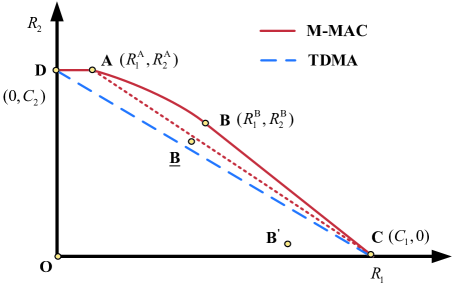
Figure 3: Structure of the capacity region of RIS-assisted SR when the direct link is present.

VI-A3 Discussions

Based on the above analysis, we plot the structure of the capacity region for the RIS-assisted SR system, as shown in Fig. 3. Points C and D represent the maximum achievable rates of the primary and secondary transmissions, illustrated in Section III and Section IV. Point A represents the rate pair A as discussed in Section VI-A1, which indicates that even though the PTx transmits signals, the secondary transmission can achieve the maximum rate. Nevertheless, at point A, the achievable rate of the primary transmission is limited since the PTx is required to transmit a constant envelope signal. Due to the existence of point A, the capacity region of the M-MAC is larger than with the conventional TDMA scheme which is achieved by the time-sharing between two transmissions with the maximum achievable rates, which can be seen in Fig. 3.

Point B in Fig. 3 represents the rate pair B, which achieves the maximum sum rate when the RIS transmits information. Since the maximum achievable rate of the primary transmission is higher than the sum rate when the RIS transmits information, the capacity region of the RIS-assisted SR is represented by closure O-D-A-B-C or the closure O-D-A-C, plotted in Fig. 3. Note that even though point B may not be on the boundary of the capacity region, e.g. the point $\underline{\mathrm{B}}$ in Fig. 3, the sum rate on point B is larger than that on point A. In Fig. 3, point $\mathrm{B}^{\prime}$ represents the rate pair based on the distributions illustrated in Proposition VI.1 when secondary signal $X_{2}$ is decoded first. Although points B and $\mathrm{B}^{\prime}$ have the same sum rate, point $\mathrm{B}^{\prime}$ is not on the capacity region boundary since the slope between points B and $\mathrm{B}^{\prime}$ is less than that between points B and C. It is worth noticing that the rate pairs on the boundary from B to C can be achieved by the time-sharing between the two transmission schemes of rate pairs B and C.

VI-B Direct Link is Absent

Here, we consider that the direct link is much weaker than the reflecting link. In this case, we can ignore the impact of the direct link. As a result, the C-Rx can only receive the signal from RIS due to the blocked direct link, whose received signal is given by

$$\bar{Y}= h_{2}X_{1}X_{2}+{Z}\triangleq h_{2}\bar{X}+{Z},$$ (26)

where $\bar{X}=X_{1}X_{2}$ is the composite signal. Due to $\mathbb{E}[|X_{1}|^{2}]\leq P$ and $|X_{2}|^{2}\leq 1$, the composite signal $\bar{X}$ should satisfy the average power constraint, i.e, $\mathbb{E}[|\bar{X}|^{2}]=\mathbb{E}[|X_{1}|^{2}]\mathbb{E}[|X_{2}|^{2}]\leq P$. Note that due to the existence of $X_{1}$, there is no peak power constraint for $\bar{X}$.

According to [26], under the average power constraint, when $\bar{X}\sim\mathcal{CN}(0,P)$, the RIS-assisted SR with the blocked direct link can achieve the maximum sum rate, which is given by

$$\bar{C}_{\mathrm{sum}}=\log(1+\frac{P|h_{2}|^{2}}{\sigma^{2}}).$$ (27)

This indicates that when $X_{1}X_{2}\sim\mathcal{CN}(0,P)$, the RIS-assisted SR can achieve the maximum sum rate. With the average power constraint of $X_{1}$ and the peak power constraint of $X_{2}$, we present the following two schemes to achieve the Gaussian distribution for $\bar{X}$.

• Scheme I: When $X_{2}=1$ and $X_{1}\sim\mathcal{CN}(0,P)$, the composite signal $\bar{X}$ follows the Gaussian distribution.

• Scheme II: When the primary signal $X_{1}$ follows the Rayleigh distribution and the secondary signal $X_{2}$ follows the uniform distribution from $-\pi$ to $\pi$ with unit power, the composite signal $\bar{X}$ follows the Gaussian distribution.

For scheme I, the RIS does not transmit information and only assists the primary transmission by passive beamforming. For scheme II, the PTx transmits the amplitude of the Gaussian signals while the RIS transmits the phase of the Gaussian signals since the amplitude of the Gaussian distribution follows the Rayleigh distribution and the phase follows the uniform distribution from $-\pi$ to $\pi$. Note that the calculation of the rates corresponding to scheme II can refer to Proposition VI.2. It is obvious that the achievable rate pair based on scheme I is one corner point on the boundary of the capacity region. To characterize the capacity region, we still need to make sure that the achievable rate pair based on scheme II is the corner point on the capacity region boundary.

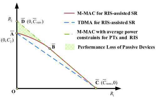
Figure 4: Structure of capacity region of RIS-assisted SR when the direct link is absent.

As shown in Fig. 4, point $\bar{\mathrm{B}}$ represents the rate pair based on scheme II. It can be found that the corner point requires to correspond to the minimum primary rate and the maximum secondary rate, under the condition that the sum rate is maximized. To achieve this, the C-Rx decodes $X_{1}$ first and then decodes $X_{2}$. From Section IV, when the SNR is low, the capacity-achieving distribution for the secondary transmission is geometrically characterized by a unit circle. This indicates that when SNR is low, point $\bar{\mathrm{B}}$ can achieve the maximum rate for the secondary transmission with the maximum sum rate. Meanwhile, when SNR is high, the capacity-achieving distribution of the amplitude of $X_{2}$ has multiple mass points. From Appendix D, we know that the composite signal $\bar{X}$ is impossible to follow Gaussian distribution when the amplitude of $X_{2}$ has multiple values. Thus, even when the SNR is high, the RIS is required to transmit phase information only to ensure that $\bar{X}$ follows Gaussian distribution. As a result, point $\bar{\mathrm{B}}$ can achieve the maximum secondary rate for any SNR, under the condition that the sum rate is maximized. Therefore, point $\bar{\mathrm{B}}$ is one corner point on the boundary of the capacity region.

When the direct link is blocked, the receiver can not recover the phase information if both PTx and RIS transmit phase signals. The main reason is that the product of $X_{1}$ and $X_{2}$ will lead to the ambiguity problem between the phase of $X_{1}$ and $X_{2}$. Therefore, different from the scenario where the direct link is present, even though the PTx transmits the constant envelop signal, the $X_{1}$ can not be decoded first, and $I(X_{1};Y)=0$. As a result, for the scenarios where the direct link is present and absent, the capacity region structures of the RIS-assisted SR are different.

From (27), it is easy to find that if the RIS satisfies the average power constraint, $\mathbb{E}[|X_{2}|^{2}]\leq 1$, the maximum achievable rate for the secondary transmission is $\log(1+\frac{P|h_{2}|^{2}}{\sigma^{2}})$, which is the same as the maximum sum rate in (27). Thus, in this case, the capacity region is a triangle, shown as the closure O-$\bar{\mathrm{C}}$-$\bar{\mathrm{D}}$ in Fig. 4. The shadow closure $\bar{\mathrm{A}}$-$\bar{\mathrm{B}}$-$\bar{\mathrm{D}}$ in Fig. 4 represents the performance loss caused by the passive nature of RIS.

VII Performance Evaluation

In this section, numerical results are presented to evaluate the capacity region of the M-MAC in the RIS-assisted SR system. The region is plotted by using the definitions in Section II-B and the derived results in Section III, IV, and V. Meanwhile, unless specified otherwise, we set $|h_{1}|^{2}=1$ and $|g_{k}\tilde{f}_{k}|^{2}=0.003$. To reveal essential insights into RIS-assisted SR, we also plot the capacity region of the conventional TDMA scheme and the capacity of the primary transmission without the RIS, given by $\log(1+\frac{P|h_{1}|^{2}}{\sigma^{2}})$.

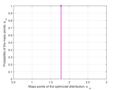
	(a) Primary signals with $\mu_{1}=0$	(b) Secondary signals with $\mu_{1}=0$
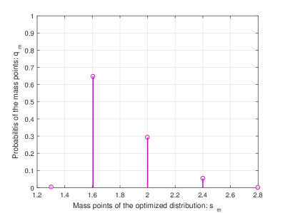
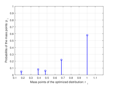
	(c) Primary signals with $\mu_{1}=0.2$	(d) Secondary signals with $\mu_{1}=0.2$
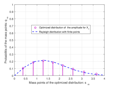
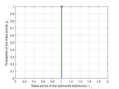
	(e) Primary signals with $\mu_{1}=0.5$	(f) Secondary signals with $\mu_{1}=0.5$

Figure 5: The optimized location of the mass points versus the corresponding probabilities for the distributions of the primary and secondary transmissions with $\mu_{1}=0$, $\mu_{1}=0.2$, and $\mu_{1}=0.5$.

Fig. 5 plots the optimized location of the mass points versus the corresponding probabilities of the distributions for both the primary and secondary transmissions with $\mu_{1}=0$, $\mu_{1}=0.2$, and $\mu_{1}=0.5$. In this figure, we set $P/\sigma^{2}=5$ dB and $K=64$. From Fig. 5 (a) and (b), we can find that when $|X_{1}|^{2}=P$, the secondary transmission can achieve its maximum rate, which is consistent with the analysis in Section VI-A1. The solid line in Fig. 5 (e) is plotted by using the PDF of the Rayleigh distribution with finite points. We can see that all the hollow circles in Fig. 5 (e) are almost scattered on the solid line. This implies that the optimized distribution of the primary transmission by maximizing the sum rate is the Gaussian distribution, which is coincident with the analysis in Section VI-A2. In addition, it is obvious that when $\mu_{1}=0.2$, the distribution of the amplitude of $X_{1}$ is discrete. This indicates that the points on the boundary of the capacity involve the continuous distribution and the discrete distribution, which verifies the necessity of introducing the expression in (16).

Figure 6: Capacity region with $K=64$.

In Fig. 6, the capacity region of the M-MAC in the RIS-assisted SR system is plotted for different $P/\sigma^{2}$. We consider that the number of the reflecting elements at the RIS is $K=64$. We can see that the higher average transmit power at the PTx can lead to a larger capacity region. Meanwhile, the capacity region of the M-MAC is always strictly convex and is larger than the traditional TDMA manner, which is coincident with the analysis in Section VI and verifies the superiority of the multiplicative multiple-access scheme. Note that the tangents of partial points on the capacity region boundary have different slopes, which is mainly related to the predesigned priorities $(\mu_{1},\mu_{2})$. The simulated structure of the capacity region is consistent with the analyzed one in Section VI, which verifies the effectiveness of the analysis.

Fig. 7 shows the capacity region of the M-MAC in the RIS-assisted SR system for the different number of reflecting elements when $P/\sigma^{2}=-5$ dB. We can find that the capacity region enlarges with the increase of $K$, which means that the strong reflecting link can enhance the rate performance for both primary and secondary transmissions. Moreover, we plot the maximum achievable rate of the primary transmission without the RIS, shown as the pentagram in Fig. 7. Interestingly, the achievable rate $R_{1}^{\mathrm{B}}$ for the primary transmission increases with $K$, and when $K$ is large, the achievable rate $R_{1}^{\mathrm{B}}$ is greater than the rate without the RIS, even though the secondary signals are unknown at the C-Rx. This fantastic phenomenon implies that different from the traditional additive MAC, when $K$ is large, the secondary transmission in the M-MAC is a beneficial composition instead of interference for the primary transmission whether the secondary signal is known or not. In addition, we can find that when $K=32$, the slopes of the rate pairs on the capacity region boundary are limited. The main reason is that the slope of the line from rate pair $(R_{1}^{\mathrm{B}},R_{2}^{\mathrm{B}})$ to rate pair $(C_{1},0)$ is higher than that from rate pair $(R_{1}^{\mathrm{A}},R_{2}^{\mathrm{A}})$ to rate pair $(C_{1},0)$ , even though the sum rate of rate pair $(R_{1}^{\mathrm{B}},R_{2}^{\mathrm{B}})$ is higher than that of rate pair $(R_{1}^{\mathrm{A}},R_{2}^{\mathrm{A}})$, which is coincident with the analysis in Section VI.

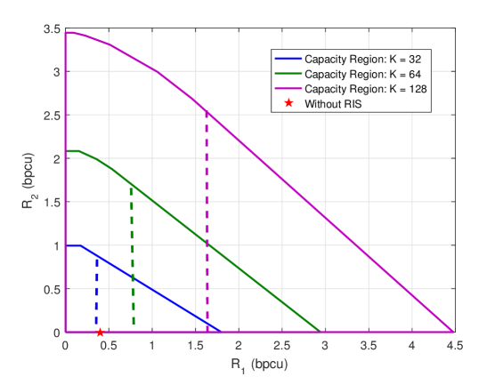
Figure 7: Capacity region with $P/\sigma^{2}=-5$ dB.

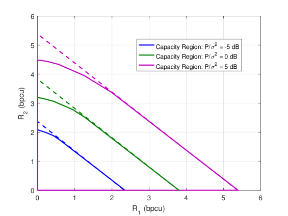
Figure 8: Capacity region when the direct link is blocked with $K=64$.

Fig. 8 shows the capacity region of the M-MAC in the RIS-assisted SR system for the different $P/\sigma^{2}$ when the direct link is weak or blocked. The number of the reflecting elements at the RIS is set to $K=64$. Similar to Fig. 6, the capacity region becomes larger with the growth of the transmit power and is larger than the traditional TDMA manner. Besides, we calculate the maximum achievable rate of the secondary transmission if the RIS satisfies the average power constraint, given by $\log(1+\frac{P|h_{2}|^{2}}{\sigma^{2}})$, which is equal to the maximum sum rate and the maximum achievable rate of the primary transmission. Thus, if the RIS satisfies the average power constraint, the capacity region, plotted using the dotted line in Fig. 8, is one triangle, which is consistent with the results in [27]. The capacity region gap between the solid and dotted lines represents the performance loss caused by the passive nature of RIS.

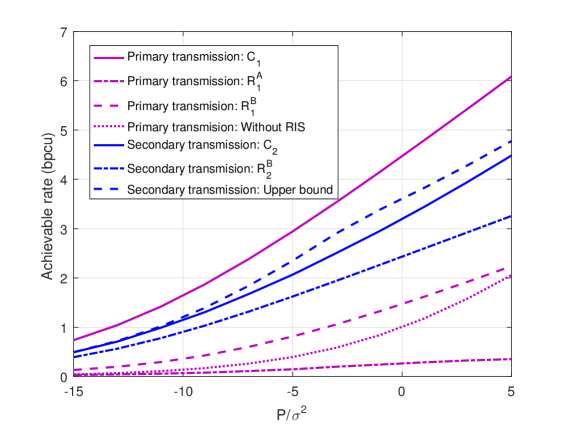
Figure 9: Achievable rates versus transmit SNR, i.e., $P/\sigma^{2}$.

Fig. 9 demonstrates the achievable rates for both primary and secondary transmissions versus $P/\sigma^{2}$ with $K=64$. Note that the calculations of $R_{1}^{\mathrm{A}}$, $R_{1}^{\mathrm{B}}$ and $R_{2}^{\mathrm{B}}$ are based on the results in Section VI-A1 and Section VI-A2. It can be found that the maximum achievable rate of the primary transmission is always greater than the rate without the RIS, which verifies the effectiveness of RIS. The achievable rates of the primary transmission $R_{1}^{\mathrm{A}}$ and $R_{1}^{\mathrm{B}}$ increase with the growth of the transmit power. In addition, rate $R_{1}^{\mathrm{B}}$ is larger than the rate without RIS, which shows the benefits from the secondary transmission to the primary transmission. Furthermore, we can find that secondary achievable rates $R_{2}^{\mathrm{B}}$ and $C_{2}$ increase with the growth of $P/\sigma^{2}$. It means that the stronger the reflecting link is, the higher the achievable rate will be, which is consistent with the analysis in Section IV. Meanwhile, the upper bound of the capacity of the secondary transmission is tight when $P/\sigma^{2}$ is small.

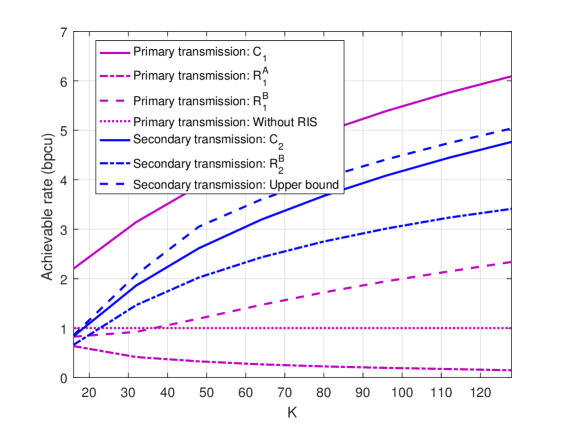
Figure 10: Achievable rates versus the number of reflecting elements, i.e., $K$.

Fig. 10 demonstrates the achievable rates for both primary and secondary transmissions versus the number of reflecting elements $K$ with $P/\sigma^{2}=0$ dB. The increase in the number of reflecting elements is equivalent to the growth of the strength of the reflecting link. From Fig. 10, it can be found that the stronger the strength of the reflecting link is, the higher the secondary transmission rates will achieve. For the primary transmission, achievable rates $C_{1}$ and $R_{1}^{\mathrm{B}}$ increase with the growth of the number of reflecting elements. For large $K$, the rate $R_{1}^{\mathrm{B}}$ is larger than the rate without RIS, which indicates that when the reflecting link is strong enough, the primary transmission can gain the benefits from the secondary transmission when the secondary signal is unknown to the decoder. Meanwhile, the rate $R_{1}^{\mathrm{A}}$ decreases with the increase of the number of reflecting elements, which can also be observed in Fig 7. The main reason is that when the reflecting link is strong enough, especially much stronger than the direct link, the phase ambiguity between $X_{1}$ and $X_{2}$ will lead to the failure in decoding $X_{1}$ first. Meanwhile, if $K\rightarrow\infty$, the capacity region of the RIS-assisted SR will approach that for the scenario where the direct link is blocked.

VIII Conclusions

This paper has investigated the characterization of the capacity region of the M-MAC in the RIS-assisted SR system. The capacity-achieving distributions of the transmitted signals at the PTx and RIS have been analyzed under the average power constraint at the PTx and the peak power constraint at the RIS. Also, the maximum achievable rates for both primary and secondary transmissions have been derived and the capacity region of the M-MAC has been characterized. Furthermore, the theoretical analysis has been performed to reveal insights into RIS-assisted SR. We have shown that the capacity region of the M-MAC is strictly convex and larger than the conventional TDMA scheme. The secondary transmission can achieve the maximum rate when the PTx transmits signals with the constant envelope. Moreover, even though the secondary signals are unknown at the C-Rx, the primary transmission in the M-MAC can achieve a higher rate than the rate without the RIS, which verifies that the primary and secondary transmissions can benefit each other. Finally, extensive numerical results have been presented to verify the accuracy of our theoretical analysis and illustrate the mutualistic relationship between the primary and secondary transmissions.

Appendix A

From (11), we have $I(X_{2};Y|X_{1})=I(X_{2};\tilde{Y})=H(\tilde{Y})-H(\tilde{Y}|X_{2})$, where $\tilde{Y}=\sqrt{P}h_{2}^{*}X_{2}+Z$. It is straightforward to have $H(\tilde{Y}|X_{2})=H(Z)=\log(\pi e\sigma^{2})$. To calculate $H(\tilde{Y})$, we use the polar coordinates of $\tilde{Y}$, which is given by $(\tilde{r},\tilde{\psi})$, where $\tilde{r}$ is the amplitude of $\tilde{Y}$ and $\tilde{\psi}$ is the phase of $\tilde{Y}$. According to the Jacobian of transformation in terms of PDF, we have $f_{\tilde{y}}(\tilde{r},\tilde{\psi})=\tilde{r}p_{\tilde{y}}(\mathrm{Re}(\tilde{y}),\mathrm{Im}(\tilde{y}))$, where $p_{\tilde{y}}$ is the PDF of $\tilde{Y}$ in the Cartesian coordinates. Hence, we have $H(\tilde{Y})=-\int_{\mathbb{C}}p_{\tilde{y}}(\mathrm{Re}(\tilde{y}),\mathrm{Im}(\tilde{y}))\log(p_{\tilde{y}}(\mathrm{Re}(\tilde{y}),\mathrm{Im}(\tilde{y})))d\tilde{y}\overset{(a)}{=}-\int_{0}^{+\infty}\int_{-\pi}^{\pi}\tilde{r}p_{\tilde{y}}(\tilde{r}\cos\tilde{\psi},\tilde{r}\sin\tilde{\psi})\log($ $p_{\tilde{y}}(\tilde{r}\cos\tilde{\psi},\tilde{r}\sin\tilde{\psi})d\tilde{\psi}d\tilde{r}=-\int_{0}^{+\infty}\int_{-\pi}^{\pi}f_{\tilde{y}}(\tilde{r},\tilde{\psi})\log(\frac{f_{\tilde{y}}(\tilde{r},\tilde{\psi})}{\tilde{r}})d\tilde{\psi}d\tilde{r},$ where $(a)$ follows from the Jacobian of transformation in terms of integration. The PDF of $\tilde{Y}$ in terms of the polar coordinates, i.e., $f_{\tilde{y}}(\tilde{r},\tilde{\psi})$, is given by

$$f_{\tilde{y}}(\tilde{r},\tilde{\psi}) =\tilde{r}p_{\tilde{r}}(\tilde{r}\cos\tilde{\psi},\tilde{r}\sin\tilde{\psi})=\tilde{r}\int_{x_{2}}f_{2}(X_{2})p_{\tilde{r}}(\tilde{r}\cos\tilde{\psi},\tilde{r}\sin\tilde{\psi}|x_{2})dx_{2}$$

$$=\int_{x_{2}}f_{2}(X_{2})\frac{\tilde{r}}{\pi\sigma^{2}}\exp\left(-\frac{|\tilde{r}e^{j\tilde{\psi}}-\sqrt{P}h_{2}^{*}x_{2}|^{2}}{\sigma^{2}}\right)dx_{2}$$

$$=\int_{-\pi}^{\pi}\sum_{\ell=1}^{L}\frac{p_{\ell}\tilde{r}}{2\pi^{2}\sigma^{2}}\exp\left(-\frac{\tilde{r}^{2}+{P}(h_{2}^{*})^{2}r_{\ell}^{2}}{\sigma^{2}}\right)\exp\left(\frac{2\tilde{r}\sqrt{P}h_{2}^{*}r_{\ell}\cos(\theta_{2}-\tilde{\psi})}{\sigma^{2}}\right)d\theta_{2}$$

$$=\sum_{\ell=1}^{L}\frac{p_{\ell}\tilde{r}}{\pi\sigma^{2}}\exp\left(-\frac{\tilde{r}^{2}+{P}(h_{2}^{*})^{2}r_{\ell}^{2}}{\sigma^{2}}\right)I_{0}\left(\frac{2\tilde{r}\sqrt{P}h_{2}^{*}r_{\ell}}{\sigma^{2}}\right),$$ (28)

where $\theta_{2}$ is the phase of $X_{2}$ and $I_{0}(x)=\frac{1}{2\pi}\int_{-\pi}^{\pi}e^{x\cos\theta}d\theta$. Then, the marginal density for $\tilde{y}$ can be obtained by integrating $\tilde{\psi}$ out of (A):

$$f_{\tilde{y}}(\tilde{r})\!=\!\int_{-\pi}^{\pi}f_{\tilde{y}}(\tilde{r},\tilde{\psi})d\tilde{\psi}=\sum_{\ell=1}^{L}\frac{2p_{\ell}\tilde{r}}{\sigma^{2}}\exp\left(-\frac{\tilde{r}^{2}+{P}(h_{2}^{*})^{2}r_{\ell}^{2}}{\sigma^{2}}\right)I_{0}\left(\frac{2\tilde{r}\sqrt{P}h_{2}^{*}r_{\ell}}{\sigma^{2}}\right)=\frac{2\tilde{r}\kappa(\tilde{r})}{\sigma^{2}},$$ (29)

where $\kappa(\tilde{r})=\sum_{\ell=1}^{L}p_{\ell}\exp\left(-\frac{\tilde{r}^{2}+{P}(h_{2}^{*})^{2}r_{\ell}^{2}}{\sigma^{2}}\right)I_{0}\left(\frac{2\tilde{r}\sqrt{P}h_{2}^{*}r_{\ell}}{\sigma^{2}}\right)$. From (A) and (29), it is easy to find that $f_{\tilde{y}}(\tilde{r},\tilde{\psi})=\frac{1}{2\pi}f_{\tilde{y}}(\tilde{r})$, which means that the amplitude and the phase of $\tilde{Y}$ are independent. Substituting (A) and (29) into $H(\tilde{Y})$, we have

$$H(\tilde{Y}) =-\int_{0}^{+\infty}f_{\tilde{y}}(\tilde{r})\log{\frac{f_{\tilde{y}}(\tilde{r})}{\tilde{r}}}d\tilde{r}+\log(2\pi)=-\int_{0}^{+\infty}\frac{2\tilde{r}\kappa(\tilde{r})}{\sigma^{2}}\log\left(\kappa(\tilde{r})\right)d\tilde{r}+\log(\pi\sigma^{2}).$$

Thus, the channel capacity of the secondary transmission is given by

$$I(X_{2};\tilde{Y})=~{}H(\tilde{Y})-\log(\pi e\sigma^{2})=-\int_{0}^{+\infty}\frac{2\tilde{r}\kappa(\tilde{r})}{\sigma^{2}}\log\left(\kappa(\tilde{r})\right)d\tilde{r}-\log(e).$$

Therefore, Theorem 2 can be proved.

Appendix B

Denote by $\theta_{1}$ the phase of $X_{1}$. The distribution of $X_{1}$ is $f_{1}(X_{1})=\frac{1}{2\pi}\sum_{m=1}^{M}q_{m}\delta(s-s_{m})$ and the distribution of $X_{2}$ is $f_{2}(X_{2}=re^{j\theta_{2}})=\frac{1}{2\pi}\sum_{\ell=1}^{L}p_{\ell}\delta(r-r_{l})$. Accordingly, the achievable rate of the primary transmission $I(X_{1};Y)$ is given by $H(Y)-H(Y|X_{1})$ and the achievable rate of the secondary transmission $I(X_{2};Y|X_{1})$ is given by $H(Y|X_{1})-H(Y|X_{1},X_{2})$. It is straightforward to have $H(Y|X_{1},X_{2})=H(Z)=\log(\pi e\sigma^{2})$. Based on Appendix A, we have

$$H({Y}|X_{1}) =H({Y}=\sqrt{P}h_{2}X_{1}X_{2}+Z|X_{1})=\int_{x_{1}}f_{1}(x_{1})H(\tilde{Y}|X_{1}=x_{1})dx_{1}$$

$$=-\sum_{m=1}^{M}q_{m}\int_{0}^{+\infty}\frac{2\tilde{r}\bar{\kappa}(\tilde{r},s_{m})}{\sigma^{2}}\log\left(\frac{2\bar{\kappa}(\tilde{r},s_{m})}{\sigma^{2}}\right)d\tilde{r}+\log(2\pi),$$ (30)

where $\bar{\kappa}(\tilde{r},s_{m})=\sum_{\ell=1}^{L}p_{\ell}\exp\left(-\frac{\tilde{r}^{2}+|h_{2}|^{2}|s_{m}|^{2}|r_{\ell}|^{2}}{\sigma^{2}}\right)I_{0}\left(\frac{2\tilde{r}|h_{2}||s_{m}||r_{\ell}|}{\sigma^{2}}\right)$. Therefore, we have $I(X_{2};Y|X_{1})=-\sum_{m=1}^{M}q_{m}\int_{0}^{+\infty}\frac{2\tilde{r}\bar{\kappa}(\tilde{r},s_{m})}{\sigma^{2}}\log\left({\bar{\kappa}(\tilde{r},s_{m})}\right)d\tilde{r}-\log(e)$.

Next, we focus on the calculation of $H(Y)$. Denote the polar coordinates of $Y$ by $(\bar{r},{\psi})$. According to the Jacobian of transformation, we have $H(Y)\!=\!-\!\int_{0}^{+\infty}\!\!\int_{-\pi}^{\pi}f_{y}(\bar{r},\psi)\log(\frac{f_{y}(\bar{r},\psi)}{\bar{r}})d\psi d\bar{r}$. To calculate $H({Y})$, we next focus on $f_{y}(\bar{r},\psi)$, which can be written as

$$f_{y}(\bar{r},\psi)=\bar{r}\int_{x_{1}}\int_{x_{2}}f_{1}(X_{1})f_{2}(X_{2})\frac{1}{\pi\sigma^{2}}\exp\left(-\frac{|\bar{r}e^{j\psi}-h_{1}x_{1}-h_{2}x_{1}x_{2}|^{2}}{\sigma^{2}}\right)dx_{1}dx_{2}$$

$$= \sum_{\ell=1}^{L}\sum_{m=1}^{M}\frac{p_{\ell}q_{m}\bar{r}}{4\pi^{3}\sigma^{2}}\int_{-\pi}^{\pi}\int_{-\pi}^{\pi}\exp\left(-\frac{|\bar{r}e^{j\psi}-|h_{1}|s_{m}e^{j(\theta_{1}+\vartheta_{1})}-|h_{2}|s_{m}r_{\ell}e^{j(\theta_{1}+\theta_{2}+\vartheta_{1})}|^{2}}{\sigma^{2}}\right)d\theta_{1}d\theta_{2},$$

$$\!=\! \sum_{\ell=1}^{L}\sum_{m=1}^{M}\frac{p_{\ell}q_{m}\bar{r}}{4\pi^{3}\sigma^{2}}\exp\!\left(\!-\frac{\bar{r}^{2}+|h_{1}|^{2}s_{m}^{2}+|h_{2}|^{2}r_{\ell}^{2}s_{m}^{2}}{\sigma^{2}}\!\right)\!\int_{-\pi}^{\pi}\!\int_{-\pi}^{\pi}\!\exp\!\left(\!\frac{-2|h_{1}||h_{2}|s_{m}^{2}r_{\ell}\cos(\theta_{2})}{\sigma^{2}}\!\right)$$

$$~{}~{}\exp\!\left(\!\frac{2\bar{r}|h_{1}|s_{m}\cos(\theta_{1}+\vartheta_{1}-\psi)}{\sigma^{2}}\!\right)\!\exp\left(\!\frac{2\bar{r}|h_{2}|s_{m}r_{\ell}\cos(\theta_{1}+\theta_{2}+\vartheta_{1}-\psi)}{\sigma^{2}}\!\right)d\theta_{1}d\theta_{2},$$ (31)

where $\vartheta_{1}$ is the phase of $h_{1}$ and the reflecting channel has the same channel phase as the direct link channel due to the design scheme of RIS. To calculate $f_{y}(\bar{r},\psi)$, we first expand $\cos(\theta_{1}+\theta_{2}+\vartheta_{1}-\psi)$ based on $\cos(\theta_{1}+\theta_{2})=\cos\theta_{1}\cos\theta_{2}-\sin\theta_{1}\sin\theta_{2}$. Accordingly, we have

$$v(\psi,\theta_{1},\theta_{2})\triangleq |h_{1}|s_{m}\cos(\theta_{1}+\vartheta_{1}-\psi)+|h_{2}|s_{m}r_{\ell}\cos(\theta_{1}+\theta_{2}+\vartheta_{1}-\psi)$$

$$= (|h_{1}|s_{m}+|h_{2}|s_{m}r_{\ell}\cos(\theta_{2}))\cos(\theta_{1}+\vartheta_{1}-\psi)-|h_{2}|s_{m}r_{\ell}\sin\theta_{2}\sin(\theta_{1}+\vartheta_{1}-\psi)$$

$$\overset{(a)}{=} \sqrt{|h_{1}|^{2}s_{m}^{2}+|h_{2}|^{2}s_{m}^{2}r_{\ell}^{2}+2|h_{1}||h_{2}|s_{m}^{2}r_{\ell}\cos(\theta_{2})}\cos(\theta_{1}+\vartheta_{1}-\psi+\alpha(\theta_{2})),$$ (32)

where $\alpha(\theta_{2})=\arctan(\frac{|h_{2}|s_{m}r_{\ell}\sin\theta_{2}}{|h_{1}|s_{m}+|h_{2}|s_{m}r_{\ell}\cos(\theta_{2})})$ and $(a)$ holds based on $a\cos(\psi)-b\sin(\psi)=\sqrt{a^{2}+b^{2}}\cos(\psi+A)$ with $\tan A=b/a$. Therefore, $f_{y}(\bar{r},\psi)$ can be simplified as

$$f_{y}(\bar{r},\psi)= \sum_{\ell=1}^{L}\sum_{m=1}^{M}\frac{p_{\ell}q_{m}\bar{r}}{4\pi^{3}\sigma^{2}}\exp\left(-\frac{\bar{r}^{2}+|h_{1}|^{2}s_{m}^{2}+|h_{2}|^{2}r_{\ell}^{2}s_{m}^{2}}{\sigma^{2}}\right)\int_{-\pi}^{\pi}\int_{-\pi}^{\pi}\exp\left(\frac{2\bar{r}v(\psi,\theta_{1},\theta_{2})}{\sigma^{2}}\right)$$

$$~{}~{}~{}~{}\exp\left(\frac{-2|h_{1}||h_{2}|s_{m}^{2}r_{\ell}\cos(\theta_{2})}{\sigma^{2}}\right)d\theta_{1}d\theta_{2}.$$ (33)

It is easy to find that $f_{y}(\bar{r})$ for ${y}$ satisfies $f_{y}(\bar{r},\psi)=\frac{1}{2\pi}f_{y}(\bar{r})$, we have

$$H({Y}) =-\int_{0}^{+\infty}f_{{y}}(\bar{r})\log{\frac{f_{\bar{y}}(\bar{r})}{\bar{r}}}d\bar{r}+\log(2\pi)=-\int_{0}^{+\infty}\frac{2\bar{r}\check{\kappa}(\bar{r})}{\sigma^{2}}\log\left(\check{\kappa}({\bar{r}})\right)d\bar{r}+\log(\pi\sigma^{2}),$$

where $\check{\kappa}(\bar{r})=\sum_{\ell=1}^{L}\frac{p_{\ell}q_{m}}{4\pi^{2}}\exp\left(-\frac{\bar{r}^{2}+|h_{1}|^{2}s_{m}^{2}+|h_{2}|^{2}r_{\ell}^{2}s_{m}^{2}}{\sigma^{2}}\right)\int_{-\pi}^{\pi}\int_{-\pi}^{\pi}$ $\exp\left(\frac{-2|h_{1}||h_{2}|s_{m}^{2}r_{\ell}\cos(\theta_{2})}{\sigma^{2}}\right)$

$\exp\left(\frac{2\bar{r}\sqrt{|h_{1}|^{2}s_{m}^{2}+|h_{2}|^{2}r_{\ell}^{2}s_{m}^{2}+2|h_{1}||h_{2}|s_{m}^{2}r_{\ell}\cos(\theta_{2})}\cos(\theta_{1}+\alpha(\theta_{2}))}{\sigma^{2}}\right)d\theta_{1}d\theta_{2}$.

According to the definition of mutual information, we have

$$I(X_{1},Y)=\sum_{m=1}^{M}q_{m}\int_{0}^{+\infty}\frac{2\tilde{r}\bar{\kappa}(\tilde{r},s_{m})}{\sigma^{2}}\log\left({\bar{\kappa}(\tilde{r},s_{m})}\right)d\tilde{r}-\int_{0}^{+\infty}\!\frac{2{r}\check{\kappa}({r})}{\sigma^{2}}\log\left(\check{\kappa}({r})\right)d{r}.$$

Therefore, Theorem 3 can be proved.

Appendix C

To calculate $I(X_{1};Y|X_{2})=H(Y|X_{2})-H(Y|X_{1},X_{2})$, we first focus on the calculation of $H(Y|X_{2})$, which is given by

$$H({Y}|X_{2}) =\int_{x_{2}}f_{2}(x_{2})H(Y|X_{2}=x_{2})dx_{2}$$

$$=-\sum_{\ell=1}^{L}p_{\ell}\int_{-\pi}^{\pi}\int_{0}^{+\infty}\frac{2\bar{r}\underline{\kappa}(\bar{r},r_{\ell},\theta_{2})}{\sigma^{2}}\log\left(\frac{2\bar{r}\underline{\kappa}(\bar{r},r_{\ell},\theta_{2})}{\sigma^{2}}\right)d\bar{r}d\theta_{2}+\log(2\pi),$$ (34)

where $\underline{\kappa}(\bar{r},r_{\ell},\theta_{2})=\sum_{m=1}^{M}q_{m}\exp\left(-\frac{\bar{r}^{2}+|h_{1}+h_{2}r_{\ell}e^{j\theta_{2}}|^{2}|s_{m}|^{2}}{\sigma^{2}}\right)$ $I_{0}\left(\frac{2\bar{r}|h_{1}+h_{2}r_{\ell}e^{j\theta_{2}}||s_{m}|}{\sigma^{2}}\right)$. Similar to Appendix B, we have

$$I(X_{1};Y|X_{2}) =H(Y|X_{2})-H(Y|X_{1},X_{2})$$

$$=-\sum_{\ell=1}^{L}p_{\ell}\int_{-\pi}^{\pi}\int_{0}^{+\infty}\frac{2\bar{r}\underline{\kappa}(\bar{r},r_{\ell},\theta_{2})}{\sigma^{2}}\log\left({\underline{\kappa}(\bar{r},r_{\ell},\theta_{2})}\right)d\bar{r}d\theta_{2}-\log(e),$$

Meanwhile, we have

$$I(X_{2};Y) =\!H(Y)\!-\!H(Y|X_{2})$$

$$=\!\sum_{\ell=1}^{L}p_{\ell}\!\int_{0}^{+\infty}\!\frac{2\bar{r}\underline{\kappa}(\bar{r},r_{\ell})}{\sigma^{2}}\!\log\left({\underline{\kappa}(\bar{r},r_{\ell})}\right)d\bar{r}-\int_{0}^{+\infty}\!\!\frac{2\bar{r}\check{\kappa}(\bar{r})}{\sigma^{2}}\!\log\left(\check{\kappa}(\bar{r})\right)d\bar{r}.$$

Therefore, Theorem 4 can be proved.

Appendix D

When $\mathbb{E}[\textit{Re}(X_{2})]\neq 0$, the amplitude and the phase of $X_{2}$ are not symmetric about the origin, respectively. For the case where the phase of $X_{2}$ does not uniformly range from $-\pi$ to $\pi$, the phases of $X_{1}$ and $X_{1}X_{2}$ are difficult to uniformly range from $-\pi$ to $\pi$ simultaneously. Thus, in this case, the phase of the virtual signal $X$ does not follow the uniform from $-\pi$ to $\pi$, which indicates that the virtual signal ${X}$ does not follow the Gaussian distribution. Similarly, for the case where the amplitude of $X_{2}$ has multiple values, the amplitude of $X_{1}X_{2}$ is difficult to follow the Rayleigh distribution, since the continuous $X_{1}$ can not compensate for the variation of $X_{2}$. In summary, when $\mathbb{E}[\textit{Re}(X_{2})]\neq 0$, ${X}$ is impossible to follow the Gaussian distribution.

Appendix E

Since $X_{1}$ follows the Gaussian distribution, it is easy to find that the received direct link signal $h_{1}X_{1}$ follows the Gaussian distribution, i.e., $h_{1}X_{1}\sim\mathcal{CN}(0,|h_{1}|^{2}P)$. When $X_{2}$ follows the circular uniform distribution, the received reflecting link signal can be written as $h_{2}X_{1}X_{2}=h_{2}se^{j(\theta 1+\theta 2)}$, where $\theta_{1}$ and $\theta_{2}$ are the phases of $X_{1}$ and $X_{2}$, respectively, and $s$ is the amplitude of $X_{1}$. Since $\theta_{1}$ and $\theta_{2}$ follow the uniform distribution from $-\pi$ to $\pi$, according to the periodicity of the trigonometric functions, it can be found that $\theta_{1}+\theta_{2}$ still follows the uniform distribution from $-\pi$ to $\pi$. As a result, $h_{2}X_{1}X_{2}$ follows the Gaussian distribution, i.e., $h_{2}X_{1}X_{2}\sim\mathcal{CN}(0,|h_{2}|^{2}P)$.

Meanwhile, we will analyze the correlation of $h_{1}X_{1}$ and $h_{2}X_{1}X_{2}$. The covariance of $h_{1}X_{1}$ and $h_{2}X_{1}X_{2}$ can be written as $\mathbb{E}[h_{1}X_{1}(h_{2}X_{1}X_{2})^{H}]=\mathbb{E}[h_{1}h_{2}^{H}|X_{1}|^{2}X_{2}^{H}]=h_{1}h_{2}^{H}\mathbb{E}[|X_{1}|^{2}]\mathbb{E}[X_{2}^{H}]=0$. Since the Gaussian variables are independent of each other when their covariance is equal to zero [40], we can find that $h_{1}X_{1}$ and $h_{2}X_{1}X_{2}$ are independent of each other. Meanwhile, the sum of two independent Gaussian variables still follows Gaussian distribution [40]. Thus, we have $X\sim\mathcal{CN}(0,P(|h_{1}|^{2}+|h_{2}|^{2}))$. Therefore, Proposition VI.1 can be proved.

Appendix F

The distribution of $X_{1}$ is $f_{1}(X_{1}=x_{1})=\frac{1}{\pi P}\exp(-\frac{|x_{1}|^{2}}{P})$ and the distribution of $X_{2}$ is $f_{2}(X_{2}=e^{j\theta_{2}})=\frac{1}{2\pi}$. Since $h_{1}X_{1}+h_{2}X_{1}X_{2}\sim\mathcal{CN}(0,P(|h_{1}|^{2}+|h_{2}|^{2}))$ from Appendix E, we have $H(Y)=\log(\pi e(P|h_{1}|^{2}+P|h_{2}|^{2}+\sigma^{2}))$. Then, $H(Y|X_{1})$ is given by

$$H(Y|X_{1}) =H({Y}=\sqrt{P}h_{2}X_{1}X_{2}+Z|X_{1})=\int_{x_{1}}f_{1}(x_{1})H(\tilde{Y}|X_{1}=x_{1})dx_{1}$$

$$=-\mathbb{E}_{x_{1}}\int_{0}^{+\infty}\int_{-\pi}^{\pi}f_{\tilde{y}}(\tilde{r},\tilde{\psi}|x_{1})\log(\frac{f_{\tilde{y}}(\tilde{r},\tilde{\psi}|x_{1})}{\tilde{r}})d\tilde{\psi}d\tilde{r},$$ (35)

To calculate $H(Y|X_{1})$, we next focus on $f_{\tilde{y}}(\tilde{r},\tilde{\psi}|x_{1})$, which can be written as

$$f_{\tilde{y}}(\tilde{r},\tilde{\psi}|x_{1})=\frac{\tilde{r}}{\pi\sigma^{2}}\exp\left(-\frac{\tilde{r}^{2}+|h_{2}|^{2}|x_{1}|^{2}}{\sigma^{2}}\right)I_{0}\left(\frac{2\tilde{r}|h_{2}||x_{1}|}{\sigma^{2}}\right).$$ (36)

It is easy to find that the marginal density $f_{y}(\bar{r})$ for ${Y}$ satisfies $f_{y}(\tilde{r},\tilde{\psi}|x_{1})=\frac{1}{2\pi}f_{y}(\tilde{r}|x_{1})$. Thus, we have

$$H({Y}|X_{1}) =-\mathbb{E}_{|x_{1}|}\int_{0}^{+\infty}f_{y}(\tilde{r}|x_{1})\log{\frac{f_{y}(\tilde{r}|x_{1})}{\tilde{r}}}d\tilde{r}+\log(2\pi)$$

$$=-\mathbb{E}_{|x_{1}|}\int_{0}^{+\infty}\frac{2\tilde{r}\tilde{\kappa}(\tilde{r},x_{1})}{\sigma^{2}}\log\left({\tilde{\kappa}(\tilde{r},x_{1})}\right)d\tilde{r}+\log(\pi\sigma^{2}),$$ (37)

where $\tilde{\kappa}(\tilde{r},x_{1})=\exp\left(-\frac{\tilde{r}^{2}+|h_{2}|^{2}|x_{1}|^{2}}{\sigma^{2}}\right)I_{0}\left(\frac{2\tilde{r}|h_{2}||x_{1}|}{\sigma^{2}}\right)$. According to the definition of mutual information, we have

$$R_{1}^{\mathrm{B}} =\log(\frac{e(P|h_{1}|^{2}+P|h_{2}|^{2}+\sigma^{2})}{\sigma^{2}})+\mathbb{E}_{|x_{1}|}\int_{0}^{+\infty}\frac{2\tilde{r}\tilde{\kappa}(\tilde{r},x_{1})}{\sigma^{2}}\log\left({\tilde{\kappa}(\tilde{r},x_{1})}\right)d\tilde{r},$$ (38)

$$R_{2}^{\mathrm{B}} =-\mathbb{E}_{|x_{1}|}\int_{0}^{+\infty}\frac{2{\tilde{r}}\tilde{\kappa}(\tilde{r},x_{1})}{\sigma^{2}}\log\left(\tilde{\kappa}(\tilde{r},x_{1})\right)d\tilde{r}-\log(e)$$ (39)

Therefore, Proposition VI.2 can be proved.

References

- [1] M. Latva-aho and K. Leppanen, “Key drivers and research challenges for 6G ubiquitous wireless intelligence,” University of Oulu, While Paper, 2019. Available: http://urn.fi/urn:isbn:9789526223544.
- [2] M. Giordani, M. Polese, M. Mezzavilla, S. Rangan, and M. Zorzi, “Toward 6G networks: Use cases and technologies,” IEEE Commun. Mag., vol. 58, no. 3, pp. 55–61, 2020.
- [3] X. You et al., “Towards 6G wireless communication networks: Vision, enabling technologies, and new paradigm shifts,” Sci. China Inf. Sci., vol. 64, no. 1, pp. 1–74, 2021.
- [4] Y.-C. Liang, Q. Zhang, E. G. Larsson, and G. Y. Li, “Symbiotic radio: Cognitive backscattering communications for future wireless networks,” IEEE Trans. Cogn. Commun. Netw., vol. 6, no. 4, pp. 1242–1255, 2020.
- [5] G. Yang, Y.-C. Liang, R. Zhang, and Y. Pei, “Modulation in the air: Backscatter communication over ambient OFDM carrier,” IEEE Trans. Commun., vol. 66, no. 3, pp. 1219–1233, Mar. 2018.
- [6] Q. Zhang, Y.-C. Liang, H.-C. Yang, and H. V. Poor, “Mutualistic mechanism in symbiotic radios: When can the primary and secondary transmissions be mutually beneficial?” IEEE Trans. Wireless Commun., vol. 21, no. 10, pp. 8036–8050, 2022.
- [7] S. Chen, Y.-C. Liang, S. Sun, S. Kang, W. Cheng, and M. Peng, “Vision, requirements, and technology trend of 6G: How to tackle the challenges of system coverage, capacity, user data-rate and movement speed,” IEEE Wireless Commun., vol. 27, no. 2, pp. 218–228, 2020.
- [8] L. Bariah, L. Mohjazi, S. Muhaidat, P. C. Sofotasios, G. K. Kurt, H. Yanikomeroglu, and O. A. Dobre, “A prospective look: Key enabling technologies, applications and open research topics in 6G networks,” IEEE Access, vol. 8, pp. 174 792–174 820, 2020.
- [9] G. Yang, Q. Zhang, and Y.-C. Liang, “Cooperative ambient backscatter communications for green Internet-of-Things,” IEEE Internet Things J., vol. 5, no. 2, pp. 1116–1130, Apr. 2018.
- [10] X. Chen, H. V. Cheng, K. Shen, A. Liu, and M.-J. Zhao, “Stochastic transceiver optimization in multi-tags symbiotic radio systems,” IEEE Internet Things J., vol. 7, no. 9, pp. 9144–9157, 2020.
- [11] Q. Zhang, H. Guo, Y.-C. Liang, and X. Yuan, “Constellation learning-based signal detection for ambient backscatter communication systems,” IEEE J. Sel. Areas Commun., vol. 37, no. 2, pp. 452–463, 2019.
- [12] H. Guo, Q. Zhang, S. Xiao, and Y.-C. Liang, “Exploiting multiple antennas for cognitive ambient backscatter communication,” IEEE Internet Things J., vol. 6, no. 1, pp. 765–775, 2019.
- [13] R. Long, Y.-C. Liang, H. Guo, G. Yang, and R. Zhang, “Symbiotic radio: A new communication paradigm for passive internet-of-things,” IEEE Internet Things J., vol. 7, pp. 1350–1363, 2020.
- [14] Z. Chu, W. Hao, P. Xiao, M. Khalily, and R. Tafazolli, “Resource allocations for symbiotic radio with finite block length backscatter link,” IEEE Internet Things J., vol. 7, no. 9, pp. 8192–8207, 2020.
- [15] T. Wu, M. Jiang, Q. Zhang, Q. Li, and J. Qin, “Beamforming design in multiple-input-multiple-output symbiotic radio backscatter systems,” IEEE Commun. Lett., vol. 25, no. 6, pp. 1949–1953, 2021.
- [16] Q. Zhang, Y.-C. Liang, and H. V. Poor, “Reconfigurable intelligent surface assisted MIMO symbiotic radio networks,” IEEE Trans. Commun., vol. 69, no. 7, pp. 4832–4846, 2021.
- [17] M. Wu, X. Lei, X. Zhou, Y. Xiao, X. Tang, and R. Q. Hu, “Reconfigurable intelligent surface assisted spatial modulation for symbiotic radio,” IEEE Trans. Veh. Technol., vol. 70, no. 12, pp. 12 918–12 931, 2021.
- [18] T. Ma, Y. Xiao, X. Lei, P. Yang, X. Lei, and O. A. Dobre, “Large intelligent surface assisted wireless communications with spatial modulation and antenna selection,” IEEE J. Sel. Areas Commun., vol. 38, no. 11, pp. 2562–2574, 2020.
- [19] R. Liu, H. Li, M. Li, and Q. Liu, “Symbol-level precoding design for intelligent reflecting surface assisted multi-user MIMO systems,” in Proc. IEEE Int. Conf. Wireless Commun. Signal Process. (WCSP). IEEE, 2019, pp. 1–6.
- [20] A. Bereyhi, V. Jamali, R. R. Müller, A. M. Tulino, G. Fischer, and R. Schober, “A single-RF architecture for multiuser massive MIMO via reflecting surfaces,” in Proc. IEEE Int. Conf. Acoustics, Speech, and Signal Process. (ICASSP). IEEE, 2020, pp. 8688–8692.
- [21] Y.-C. Liang, Q. Zhang, J. Wang, R. Long, H. Zhou, and G. Yang, “Backscatter communication assisted by reconfigurable intelligent surfaces,” Proc. IEEE, vol. 110, no. 9, pp. 1339–1357, 2022.
- [22] M. Hua, Q. Wu, L. Yang, R. Schober, and H. V. Poor, “A novel wireless communication paradigm for intelligent reflecting surface based symbiotic radio systems,” IEEE Trans. Signal Process., vol. 70, pp. 550–565, 2021.
- [23] H. Zhou, X. Kang, Y.-C. Liang, S. Sun, and X. Shen, “Cooperative beamforming for reconfigurable intelligent surface-assisted symbiotic radios,” IEEE Trans. Veh. Technol., DOI: 10.1109/TVT.2022.3190515, 2022.
- [24] Q. Zhang, Y.-C. Liang, and H. V. Poor, “Symbiotic radio: A new application of largeintelligent surface/antennas (LISA),” Proc. IEEE Wireless Commun. Netw. Conf. (WCNC), May 2020.
- [25] D. Tse and P. Viswanath, Fundamentals of Wireless Communication. Cambridge university press, 2005.
- [26] T. M. Cover, Elements of Information Theory. John Wiley & Sons, 1999.
- [27] S. R. B. Pillai, “On the capacity of multiplicative multiple access channels with AWGN,” in IEEE Inf. Theory Workshop. IEEE, 2011, pp. 452–456.
- [28] J. G. Smith, “The information capacity of amplitude-and variance-constrained scalar Gaussian channels,” Inf. Control, vol. 18, no. 3, pp. 203–219, 1971.
- [29] S. Shamai and I. Bar-David, “The capacity of average and peak-power-limited quadrature Gaussian channels,” IEEE Trans. Inf. Theory, vol. 41, no. 4, pp. 1060–1071, 1995.
- [30] A. Dytso, M. Al, H. V. Poor, and S. S. Shitz, “On the capacity of the peak power constrained vector Gaussian channel: An estimation theoretic perspective,” IEEE Trans. Inf. Theory, vol. 65, no. 6, pp. 3907–3921, 2019.
- [31] B. Mamandipoor, K. Moshksar, and A. K. Khandani, “Capacity-achieving distributions in Gaussian multiple access channel with peak power constraints,” IEEE Trans. Inf. Theory, vol. 60, no. 10, pp. 6080–6092, 2014.
- [32] O. Ozel and S. Ulukus, “On the capacity region of the Gaussian MAC with batteryless energy harvesting transmitters,” in IEEE GLOBECOM. IEEE, 2012, pp. 2385–2390.
- [33] W. Liu, Y.-C. Liang, Y. Li, and B. Vucetic, “Backscatter multiplicative multiple-access systems: Fundamental limits and practical design,” IEEE Trans. Wireless Commun., vol. 17, no. 9, pp. 5713–5728, 2018.
- [34] Q. Zhang, L. Zhang, Y.-C. Liang, and P. Kam, “Backscatter-NOMA: A symbiotic system of cellular and Internet-of-Things networks,” IEEE Access, vol. 7, pp. 20 000–20 013, 2019.
- [35] G. Dumphart, J. Sager, and A. Wittneben, “Load modulation for backscatter communication: Channel capacity and capacity-approaching finite constellations,” arXiv preprint arXiv:2207.08100, 2022.
- [36] R. Karasik, O. Simeone, M. Di Renzo, and S. Shamai, “Single-RF multi-user communication through reconfigurable intelligent surfaces: An information-theoretic analysis,” in IEEE Int. Symp. Inf. Theory (ISIT), 2021, pp. 2352–2357.
- [37] J. Ye, S. Guo, S. Dang, B. Shihada, and M.-S. Alouini, “On the capacity of reconfigurable intelligent surface assisted MIMO symbiotic communications,” IEEE Trans. Wireless Commun., vol. 21, no. 3, pp. 1943–1959, 2021.
- [38] A. Thangaraj, G. Kramer, and G. Böcherer, “Capacity bounds for discrete-time, amplitude-constrained, additive white Gaussian noise channels,” IEEE Trans. Inf. Theory, vol. 63, no. 7, pp. 4172–4182, 2017.
- [39] A. Goldsmith, S. A. Jafar, N. Jindal, and S. Vishwanath, “Capacity limits of MIMO channels,” IEEE J. Sel. Areas Commun., vol. 21, no. 5, pp. 684–702, 2003.
- [40] R. V. Hogg, J. McKean, and A. T. Craig, Introduction to Mathematical Statistics. Pearson Education, 2005.