The spin and mass ratio affects the gravitational waveforms of binary black hole mergers with a total system mass of 12-130
Abstract
Analyzing the observations obtained by the LIGO Scientific Collaboration and the Virgo Collaboration, a new era has begun in binary black hole (BBH) merger processes and black hole physics studies. The fact that very massive stars that will become black holes at the end of their evolution are in binary or multiple states adds particular importance to BBH studies. In this study, using the SEOBNRv4_opt gravitational waveform model developed for compact binary systems, many () models were produced under different initial conditions, and the pre- and post-merge parameters were compared. In the models, it is assumed that the initial total mass (Mtot) of the binary systems varies between 12-130 with step interval 1, the mass ratios () vary between 1 and 2 with step interval 0.004, and the initial spin () value varies between and with step interval 0.017. Final spin (), fractional mass loss (MFL), and the maximum gravitational wave amplitude (hmax) obtained during the merger were compared with appropriate tables and figures obtained from the results of the relativistic numeric model obtained according to the initial parameters. Our results show that the fractional mass loss (MFL) in generated BBH coalescences varied about 2.7 to 9.2%, and the final spin value () between 0.29 and 0.91. In most of the BBHs we have modeled, we found that MFL varies inversely with . However, it has been found that MFL values are not always inversely varied to the parameter in systems of opposite initial spin, where the large mass black hole component is positively oriented. Accordingly, it is understood that the values of MFL decrease to a certain point of and then increase according to the increasing direction of . We also discussed and catalogued these obtained results with the initial parameter sets in four tables.
keywords:
black holes, gravitational waves, binaries, High Energy Astrophysical Phenomenav#1
1 Introduction
Einstein obtained equations in 1916 describing a gravitational field in space-time geometry according to the General Relativity (GR) (1916AnP…354..769E, ). He solved the field equations, named after him, for some quantities of perturbations in space-time under certain conditions. Einstein revealed that these solutions correspond to the wave equations. From this point of view, Einstein predicted any perturbations that occurred in space-time can propagate in the form of waves at the speed of light (1916SPAW…….688E, ). After that, such waves were called gravitational waves (GWs). Binary black holes (BBHs) are one of the important astrophysical objects that can be modelled as GW sources. The theoretical studies on the evolution of BBHs continued and many advances have been made in numerical relativity (NR) studies of BBH simulations. At last, the gravitational waveform evolution of a BBH merger has been fully obtained by Pretorius (2005PhRvL..95l1101P, ) for the first time.
GW signals contain lots of data about the astrophysical systems that cannot be obtained from the electromagnetic spectrum. Also, these analyses are used for consistency tests of the GR in strong gravitational fields (2016PhRvL.116v1101A, ; 2019CQGra..36n3001B, ). By comparing the obtained GW observation data with the wave models calculated within the framework of the GR, various information about the physical parameters of the wave sources is obtained. In the research area known as parameter estimation (2019CQGra..36n3001B, ; 2013PhRvD..88f2001A, ; 2009CQGra..26k4007R, ; 2009CQGra..26t4010V, ; 2013PhRvD..87l2002S, ), suitable waveforms with sufficient sensitivity are produced to determine the physical parameters of the wave sources using observation data of the GWs.
In GR, due to the lack of analytical solutions for the evolution of the BBHs, numerical solutions and some approximation methods have been developed for the production of waveforms, used in the parameter estimation within the framework of NR. By making numerical solutions of GR according to many different parameters, the modeled gravitational waveforms can be produced with sufficient accuracy (2009PhRvD..79b4003S, ; 2012CQGra..29d5003L, ; 2012PhRvD..86h4033B, ; 2015PhRvD..92j4028O, ; 2014CQGra..31k5004A, ; 2010APS..NWS.H1012D, ; 2013APS..APRC10004T, ; 2013CQGra..31b5012H, ). However, especially for BBHs, the numerical solutions, used in the production of waveforms, require high performance computers. Also, these calculations can take days or even weeks for a single parameter set. Therefore, many approximation models have been developed to produce accurate waveforms quickly and reliably according to various parameter sets. These models are arranged into three main groups: post Newtonian (PN) (2006LRR…..9….4B, ; poisson2014gravity, ), Phenomenological (phenom) (2007CQGra..24S.689A, ; 2011PhRvL.106x1101A, ; 2016PhRvD..93d4007K, ; 2014PhRvL.113o1101H, ), and the effective-one-body (EOB) (1999PhRvD..59h4006B, ; 2011PhRvD..84l4052P, ; 2012PhRvD..86b4011T, ; 2014PhRvD..89f1502T, ; 2014PhRvD..89h4006P, ) approaches. Phenom and EOB models can be used to model the inspiral, merger, and ring-down phase of the BBH systems. However, the PN type approach models can only generate gravitational waveforms for the early inspiral phase. Since the sensitivity of the ground-based GW detectors will be increased in the coming years, many studies are underway to develop Phenom and EOB waveform models (2017CQGra..34j4002A, ; 2013PhRvD..87j4003L, ; 2015PhRvD..92j2001K, ). In addition to these approach models, some EOB-based waveform models are developed by using the reduced-order modeling (ROM) techniques (prudhomme:hal-00798326, ; BARRAULT2004, ; 2011PhRvL.106v1102F, ; 2014PhRvX…4c1006F, ) for numerical solutions of the BBHs in high-performance computers. These waveform models (produced by ROM techniques) are called surrogate-waveform models (2017PhRvD..96b4058B, ).
Today, some codes have been developed that run the mentioned approach models. Among these codes, Python Compact Binary Coalescence (PyCBC) code (alex_nitz_2019_3265452, ), which was developed and used by the LIGO/Virgo team, produces waveforms of the BBHs according to various parameters using approach models. In this study, PyCBC code was used in the generation of waveform models of BBHs according to the determined parameter sets.
In Section 2, detailed information about the GW observations used in some plots of this study was given. In the section 3, the importance of the waveform models used in the analysis of the observation data was emphasised, and NR simulation studies in this field were given. Also, the selected approach models were outlined and some comparison studies between approximation models and observation data are given as an example. In the section 4, according to various parameters such as initial spin directions and chirp-mass (1996CQGra..13..575B, ) of the BBHs, the approximation models which are suitable for our purpose were determined and some interesting results were obtained as a result of these studies. In the final section 5, possible initial conditions for the observed systems have been treated. Also, in the section A, other tables made for this study were left online.
2 Observation of GWs from BBH Mergers
Direct observations of GWs started with the observation of a BBH system called GW150914 by LIGO detectors (2016PhRvL.116f1102A, ). Following the first GW observation, two more BBH merger systems were observed during the run. These are named GW151012 (2019PhRvX…9c1040A, ) and GW151226 (2016PhRvL.116x1103A, ). Also, the first four GW observations made during the run could only be made with LIGO detectors, and these observations were found to belong to BBH merger systems of GW170104 (2017PhRvL.118v1101A, ), GW170608 (2017ApJ…851L..35A, ), GW170729 (2019PhRvX…9c1040A, ), and GW170809 (2019PhRvX…9c1040A, ).
Within the first 10 BBHs observed, the less massive system was determined to be GW170608. Just after this observation, GW170729 was recorded as the most massive and distant BBH system. Following this event, technical improvements of the Virgo detector were completed and observations started as the third GW detector with the LIGO. The observations made by LIGO and Virgo detectors together are as follows GW170814 (2017PhRvL.119n1101A, ), GW170817 (2017PhRvL.119p1101A, ), GW170818 (2019PhRvX…9c1040A, ), and GW170823 (2019PhRvX…9c1040A, ). Consequently, a total of 11 GW observations were performed during the and runs. Ten of these observations belong to the BBHs. Unlike these observations, the GW170817 is the first GW observation of a binary neutron star system. GRB170817A gamma-ray burst was also observed simultaneously in the electromagnetic spectrum related to this observation (2017ApJ…848L..13A, ). In the period covering April - October 2019, 39 new observations were made and published as GWTC-2 (2021PhRvX..11b1053A, ). Most of these observations have produced binary black hole observations. However, binary neutron stars and the first neutron star-black hole binary systems have also been observed.
The mass of the component BHs of systems, the final mass Mf, and the final spin are given in Table 1. The data listed in the Table 1 are taken from the GWTC catalogues. Other observations, such as GW150914, appear to have been published as single articles. Therefore, some of the data written in Table 1 are taken from these individual observation articles. (The references of all these observations are given in this study). We have shown them in the Figures [1 - 4] to show their compatibility. All BBHs observed in the , runs and some BBHs of the run are added. These observations are; GW190408_181802, GW190413_052954, GW190512_180714, GW190517_055101, GW190630_185205 and GW190910_112807 (2021PhRvX..11b1053A, ; 2021PhRvD.103l2002A, ). Since the observational systems were selected according to the parameter ranges used for the gravitational waveform studies in the section 4, not all of the systems observed in the period could be included.
| Name | id | ||||
|---|---|---|---|---|---|
| GW150914 | G1 | 35.6 | 30.6 | 63.1 | 0.69 |
| GW151012 | G2 | 23.2 | 13.6 | 35.6 | 0.67 |
| GW151226 | G3 | 13.7 | 7.7 | 20.5 | 0.74 |
| GW170104 | G4 | 30.8 | 20.0 | 48.9 | 0.66 |
| GW170608 | G5 | 11.0 | 7.6 | 17.8 | 0.69 |
| GW170729 | G6 | 50.2 | 34.0 | 79.5 | 0.81 |
| GW170809 | G7 | 35.0 | 23.8 | 56.3 | 0.70 |
| GW170814 | G8 | 30.6 | 25.2 | 53.2 | 0.72 |
| GW170818 | G9 | 35.4 | 26.7 | 59.4 | 0.67 |
| GW170823 | G10 | 39.5 | 29.0 | 65.4 | 0.72 |
| GW190408_181802 | G11 | 24.6 | 18.4 | 41.1 | 0.67 |
| GW190413_052954 | G12 | 34.7 | 23.7 | 56.0 | 0.68 |
| GW190512_180714 | G13 | 23.3 | 12.6 | 34.5 | 0.65 |
| GW190517_055101 | G14 | 37.4 | 25.3 | 59.3 | 0.87 |
| GW190630_185205 | G15 | 35.1 | 23.7 | 56.4 | 0.70 |
| GW190910_112807 | G16 | 43.9 | 35.6 | 75.8 | 0.70 |
3 A Case Study: Use of Some Approximation Models with Observational Data
The main purpose of this section is to show a sample study on how gravitational waveform approximation models are used in the analysis of observational data. As the gravitational waveform approximation model, SEOBNRv4_opt model (2017PhRvD..95d4028B, ) and NRSur7dq2 approximation model (2017PhRvD..96b4058B, ) were used. GW150914 observation data was used as the observation data. SEOBNRv4_opt (Spinning Effective One-Body Numerical Relativity) is an EOB-based GW approximation model. The EOB formalism is an analytical approach to the gravitational two-body problem in GR. It aims to describe all the different phases of the two-body dynamics in a single analytical method.
NRSur7dq2 model, which is compatible with GW150914 observation data, is a surrogate model for GWs from NR simulations of BBHs, and it is a ROM (Reduced Ordering Model) (2014PhRvX…4c1006F, ) based GW approximation model. This approximation model has been developed for GW modeling of BBHs with a 7-dimensional parameter space (3-dimensional spin parameters of each component BH and mass ratio of the system) and covers spin magnitudes up to 0.8 and mass ratios up to 2. We just wanted to compare both approaches based on different foundations and see how well these models fit the observation data in this section. However, NRSur7dq2 model was not used in the studies in section 4, as it is not suitable for producing waveform of BBHs with a total mass of less than 60 .
We obtained H1 detector raw data of 32 seconds-long at 16 kHz resolution from the Gravitational Wave Open Science Center (GWOSC) (2019arXiv191211716T, ; gwosc, ). To compare the observed data and the SEOBNRv4_opt waveform model data, some processes called ”whitening and smoothing” were performed with the help of PyCBC signal processing codes. The whitening and smoothing terms are generally used in signal image processing and are related to filtering the signal data in desired frequency ranges by removing noise. For the processing of raw gravitational wave data, the methods described on the official site of PyCBC were used smoothed_strain . Accordingly, the power spectral density (PSD) value of the raw data is calculated using Welch’s method 1161901 first. The whitening process is obtained by converting the raw observation data to the frequency series and dividing it by the square root of the PSD. The smoothing process is the filtering of the whitened data in a specific frequency range according to the technical specifications of the detector and other known different environmental noise sources.
The matched-filtering signal-processing method (1999PhRvD..60b2002O, ) was implemented on raw observed data by the \codewordmatched_filter() function of the PyCBC code. In addition, some of the codes of the PyCBC, such as high pass filtering \codewordhighpass() (bandpass, ), have been used since the noises of the frequencies of less than 15 Hz is dominant on the observation data. The signal processes on raw GW data mentioned above were adapted using similar PyCBC tutorials (signal_tutorials, ). Also, some Python codes, that produce templates to fit the observation data for comparison from the SEOBNRv4_opt and NRSur7dq2 waveform models, were written (by following the instructions in (signal_tutorials, )) by us to compare for the purposes of the study. Finally, the merge-time (GPS time (gpstime, )) and the signal to noise ratio (SNR) were found using \codewordmatched_filter() function of PyCBC for GW150914’s observation data. To calculate the SNR value of the raw observation data, templates are first created by using SEOBNRv4_opt and NRSur7dq2 models. For this, we use PyCBC code and import \codewordget_fd_waveform() and generate a template as a frequency series \codewordFrequencySeries(). So, we import the \codewordmatched_filter() method, and pass it our templates, the observation data, and the PSD.
Finally, SNR was found to be 19.68 at 1126259462.425 s for SEOBNRv4_opt and 19.62 at 1126259462.423 s for NRSur7dq2. The aim of the studies in this section is to convey some processes about how the SEOBNRV4_opt model, which we use to generate waveforms according to certain parameter sets, is used with observational data. This study was not done to prove that the SEOBNRv4_opt model or NRSur7dq2 are successful. The necessary information regarding the performance of these models are specified in the relevant references.
4 Produced BBH models and some unusual results
In this section, the final spin () and the final mass Mf parameters were investigated by using SEOBNRv4 waveform model (2017PhRvD..95d4028B, ) according to various initial spin and mass ratio parameter values. For the reliability of the data produced with the SEOBNRv4_opt waveform model, the uncertainty (unfaithfulness) of the data is less than (2017PhRvD..95d4028B, ). It was determined that the final parameter values changed unusually according to some initial parameter sets. Therefore, in the waveform data made for this study, to examine these unusual changes, only spin-aligned (i.e., the spin directions of the modelled BBH components were chosen to be perpendicular to the orbital plane) situations were considered by using a simple approach in the initial spin parameters. Thus, the SEOBNRv4_opt waveform model was used to determine the final parameters resulting from the evolution of BBHs. In our produced GW waveform data, the total mass parameters were limited to in the range 12 and 130 with the step intervals . The initial component mass of the modeled systems were represented as . Mass ratios were limited to and step intervals . The initial spin directions of the systems are positive in the same direction as the orbital angular momentum and negative in the opposite direction. The spin intervals were limited to step and values. Also, the initial spin magnitudes of the BHs forming the systems due to the size of the data obtained from the models were taken as . The distance parameter was taken as . The orbital inclination angle of the systems was taken as , i.e., face-on view, in which the wave amplitudes reach the maximum value. Consequently, we wrote new codes in the Python programming language to use the SEOBNRv4_opt waveform model for these selected parameter ranges.
The produced model data were simply grouped and analysed in four different categories according to the initial spin directions of the BHs forming the components of the systems. The first of these categories is Both Positive case) where both component BHs have positive spin directions, i.e., the same direction of the orbital angular momentum. The second category is (Primary Positive case) which includes cases where the massive BH has positive and the other one has negative initial spins. The third category (Primary Negative case) is the opposite spins of . The fourth category is (Both Negative case), where both components are negative.
To analyze the modeled BBHs data according to the different parameter sets mentioned above, four different appropriate plot types were determined. In the parameter settlements made on the plots, data from the initial parameters of the modeled systems, are placed on the x-axis. These initial parameters are the initial mass ratios , and the initial spin values of the component BHs , . The final parameters of the systems are fractional mass loss M, and spin magnitude of the remnant BH.
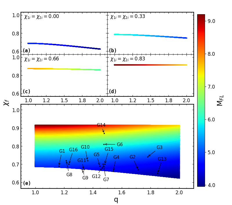
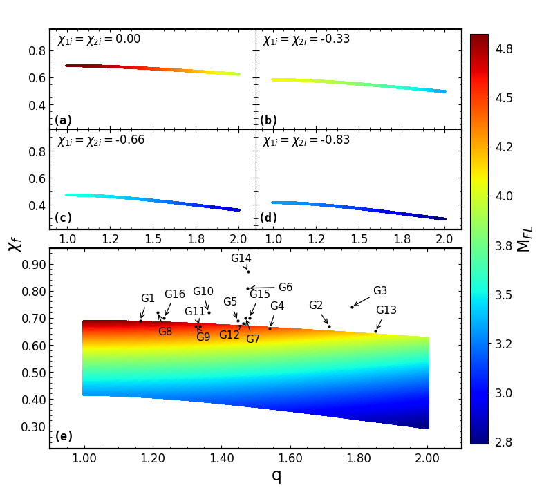


It is aimed to show the parameter changes numerically by giving the generated waveform data briefly in Tables 2, 3, 4, and 5. Numerical data generated from SEOBNRv4_opt are shown for models in Table 2. Furthermore, the plots according to , and cases are shown in Figures [2 - 4] and numerical data are given in Tables [3 - 5].
Variations of parameters of the modelled systems (i.e., the produced gravitational waveforms of BBHs according to certain parameter sets in this study.) with respect to and MFL distributions of the systems are shown in Figures [1 - 4] All of these 4 figures consist of 5 panels. In the panels on these figures, modelled systems are shown collectively in the range. In addition, , , and panels are plotted by single initial spin value. Also, the observation data from Table 1 are dotted on the plot. Accordingly, it is seen that the parameters of the BHs with large initial spins have large values as it’s supposed to be in GWOSC results (2019arXiv191211716T, ) and relevant numerical data can be seen from Table 2. In addition, the computed fractional mass losses MFL reached maximum values of , which is inversely varied with the and varied with the parameters. Furthermore, in Figures 1 and 2 show that there is a relationship between parameter and MFL.
It is understood from Tables [3, 4] that parameter is independent of in systems with the equal mass components of and cases. In such states, it can be seen that MFL parameter is not affected by changes. Therefore, in systems that have similar component mass and opposite initial spin-sign (i.e., component black holes have opposite spins relative to each other.), it can be thought that the spin vectors of the components are not affected by changes since the parameters cancel out each other.
Variations of the , Mtot and parameters of the produced GW waveform data were obtained from the SEOBNRv4_opt and some of the results were given in Table [2 - 5]. Accordingly, it is understood from the tables and plots that and MFL parameters obtained from all modelled systems except , are inversely changed with .
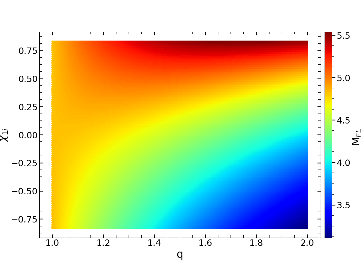
However, when Figure 4 is examined, there is a linear relationship between and with spin. In the same plot, it is seen that MFL parameter shows a linear relationship, up to certain values depending on spin values and inversely varied change for subsequent values due to initial spins. In order to better analyse these situations in models based on parameters, Figure 5 (including models), is plotted. In Figure 5, it is seen that MFL parameter have turning-points according to certain values for the condition . Particularly in the region , the changing trends become more efficient. The MFL values of corresponding values where trend-turning occurred are underlined in Table 3. Accordingly, it was found that MFL increased to maximum value up to at and tend to decrease after .
From Table 2, the maximum final spin value could occur in case. Likewise, the maximum fractional mass loss is also found to be M in . In all modelled data, the systems with a minimum value of and MFL parameters are examined in the case of . When top panel of Figure 2 and Table 5 are examined for , it is seen that the systems have minimum values at and M.
| Mtot/M⊙ | 1.00 | 1.10 | 1.20 | 1.30 | 1.40 | 1.50 | 1.60 | 1.70 | 1.80 | 1.90 | 2.00 | ||
|---|---|---|---|---|---|---|---|---|---|---|---|---|---|
| 0.00 | 15 | hmax | 0.179 | 0.178 | 0.177 | 0.175 | 0.173 | 0.170 | 0.168 | 0.164 | 0.161 | 0.159 | 0.156 |
| MFL | 4.821 | 4.803 | 4.754 | 4.683 | 4.596 | 4.498 | 4.394 | 4.285 | 4.174 | 4.062 | 3.951 | ||
| 0.686 | 0.685 | 0.682 | 0.677 | 0.671 | 0.664 | 0.656 | 0.648 | 0.640 | 0.632 | 0.623 | |||
| 30 | hmax | 0.357 | 0.356 | 0.354 | 0.350 | 0.346 | 0.340 | 0.335 | 0.330 | 0.324 | 0.318 | 0.312 | |
| MFL | 4.821 | 4.803 | 4.754 | 4.683 | 4.596 | 4.498 | 4.394 | 4.285 | 4.174 | 4.062 | 3.951 | ||
| 0.686 | 0.685 | 0.682 | 0.677 | 0.671 | 0.664 | 0.656 | 0.648 | 0.640 | 0.632 | 0.623 | |||
| 60 | hmax | 0.714 | 0.712 | 0.707 | 0.700 | 0.691 | 0.681 | 0.670 | 0.659 | 0.647 | 0.636 | 0.624 | |
| MFL | 4.821 | 4.803 | 4.754 | 4.683 | 4.596 | 4.498 | 4.394 | 4.285 | 4.174 | 4.062 | 3.951 | ||
| 0.686 | 0.685 | 0.682 | 0.677 | 0.671 | 0.664 | 0.656 | 0.648 | 0.640 | 0.632 | 0.623 | |||
| 90 | hmax | 1.071 | 1.068 | 1.061 | 1.050 | 1.037 | 1.022 | 1.006 | 0.989 | 0.971 | 0.954 | 0.936 | |
| MFL | 4.821 | 4.803 | 4.754 | 4.683 | 4.596 | 4.498 | 4.394 | 4.285 | 4.174 | 4.062 | 3.951 | ||
| 0.686 | 0.685 | 0.682 | 0.677 | 0.671 | 0.664 | 0.656 | 0.648 | 0.640 | 0.632 | 0.623 | |||
| 0.33 | 15 | hmax | 0.179 | 0.178 | 0.177 | 0.175 | 0.173 | 0.170 | 0.167 | 0.165 | 0.162 | 0.159 | 0.156 |
| MFL | 5.934 | 5.910 | 5.849 | 5.760 | 5.651 | 5.529 | 5.399 | 5.263 | 5.124 | 4.985 | 4.846 | ||
| 0.784 | 0.784 | 0.782 | 0.779 | 0.775 | 0.771 | 0.766 | 0.761 | 0.756 | 0.751 | 0.745 | |||
| 30 | hmax | 0.357 | 0.356 | 0.354 | 0.350 | 0.346 | 0.341 | 0.335 | 0.330 | 0.324 | 0.318 | 0.312 | |
| MFL | 5.934 | 5.910 | 5.849 | 5.760 | 5.651 | 5.529 | 5.399 | 5.263 | 5.124 | 4.985 | 4.846 | ||
| 0.784 | 0.784 | 0.782 | 0.779 | 0.775 | 0.771 | 0.766 | 0.761 | 0.756 | 0.751 | 0.745 | |||
| 60 | hmax | 0.715 | 0.713 | 0.708 | 0.700 | 0.692 | 0.682 | 0.671 | 0.660 | 0.648 | 0.636 | 0.625 | |
| MFL | 5.934 | 5.910 | 5.849 | 5.760 | 5.651 | 5.529 | 5.399 | 5.263 | 5.124 | 4.985 | 4.846 | ||
| 0.784 | 0.784 | 0.782 | 0.779 | 0.775 | 0.771 | 0.766 | 0.761 | 0.756 | 0.751 | 0.745 | |||
| 90 | hmax | 1.072 | 1.069 | 1.062 | 1.051 | 1.037 | 1.022 | 1.006 | 0.989 | 0.972 | 0.955 | 0.937 | |
| MFL | 5.934 | 5.910 | 5.849 | 5.760 | 5.651 | 5.529 | 5.399 | 5.263 | 5.124 | 4.985 | 4.846 | ||
| 0.784 | 0.784 | 0.782 | 0.779 | 0.775 | 0.771 | 0.766 | 0.761 | 0.756 | 0.751 | 0.745 | |||
| 0.66 | 15 | hmax | 0.180 | 0.179 | 0.178 | 0.176 | 0.174 | 0.171 | 0.168 | 0.166 | 0.163 | 0.160 | 0.157 |
| MFL | 7.762 | 7.731 | 7.649 | 7.530 | 7.385 | 7.223 | 7.048 | 6.867 | 6.683 | 6.498 | 6.314 | ||
| 0.874 | 0.874 | 0.873 | 0.872 | 0.871 | 0.869 | 0.868 | 0.866 | 0.864 | 0.862 | 0.860 | |||
| 30 | hmax | 0.360 | 0.359 | 0.356 | 0.352 | 0.348 | 0.343 | 0.337 | 0.332 | 0.326 | 0.320 | 0.314 | |
| MFL | 7.762 | 7.731 | 7.649 | 7.530 | 7.385 | 7.223 | 7.048 | 6.867 | 6.683 | 6.498 | 6.314 | ||
| 0.874 | 0.874 | 0.873 | 0.872 | 0.871 | 0.869 | 0.868 | 0.866 | 0.864 | 0.862 | 0.860 | |||
| 60 | hmax | 0.719 | 0.717 | 0.712 | 0.705 | 0.696 | 0.686 | 0.675 | 0.664 | 0.652 | 0.640 | 0.628 | |
| MFL | 7.762 | 7.731 | 7.649 | 7.530 | 7.385 | 7.223 | 7.048 | 6.867 | 6.683 | 6.498 | 6.314 | ||
| 0.874 | 0.874 | 0.873 | 0.872 | 0.871 | 0.869 | 0.868 | 0.866 | 0.864 | 0.862 | 0.860 | |||
| 90 | hmax | 1.079 | 1.076 | 1.069 | 1.058 | 1.044 | 1.029 | 1.012 | 0.995 | 0.978 | 0.960 | 0.942 | |
| MFL | 7.762 | 7.731 | 7.649 | 7.530 | 7.385 | 7.223 | 7.048 | 6.867 | 6.683 | 6.498 | 6.314 | ||
| 0.874 | 0.874 | 0.873 | 0.872 | 0.871 | 0.869 | 0.868 | 0.866 | 0.864 | 0.862 | 0.860 | |||
| 0.83 | 15 | hmax | 0.181 | 0.181 | 0.179 | 0.177 | 0.175 | 0.172 | 0.170 | 0.167 | 0.164 | 0.161 | 0.158 |
| MFL | 9.204 | 9.166 | 9.068 | 8.925 | 8.751 | 8.556 | 8.347 | 8.130 | 7.909 | 7.688 | 7.468 | ||
| 0.915 | 0.915 | 0.915 | 0.915 | 0.915 | 0.915 | 0.915 | 0.914 | 0.914 | 0.914 | 0.914 | |||
| 30 | hmax | 0.362 | 0.361 | 0.359 | 0.355 | 0.350 | 0.345 | 0.339 | 0.334 | 0.328 | 0.322 | 0.316 | |
| MFL | 9.204 | 9.166 | 9.068 | 8.925 | 8.751 | 8.556 | 8.347 | 8.130 | 7.909 | 7.688 | 7.468 | ||
| 0.915 | 0.915 | 0.915 | 0.915 | 0.915 | 0.915 | 0.915 | 0.914 | 0.914 | 0.914 | 0.914 | |||
| 60 | hmax | 0.724 | 0.722 | 0.717 | 0.710 | 0.700 | 0.690 | 0.679 | 0.667 | 0.656 | 0.644 | 0.632 | |
| MFL | 9.204 | 9.166 | 9.068 | 8.925 | 8.751 | 8.556 | 8.347 | 8.130 | 7.909 | 7.688 | 7.468 | ||
| 0.915 | 0.915 | 0.915 | 0.915 | 0.915 | 0.915 | 0.915 | 0.914 | 0.914 | 0.914 | 0.914 | |||
| 90 | hmax | 1.086 | 1.083 | 1.076 | 1.064 | 1.051 | 1.035 | 1.019 | 1.001 | 0.983 | 0.966 | 0.948 | |
| MFL | 9.204 | 9.166 | 9.068 | 8.925 | 8.751 | 8.556 | 8.347 | 8.130 | 7.909 | 7.688 | 7.468 | ||
| 0.915 | 0.915 | 0.915 | 0.915 | 0.915 | 0.915 | 0.915 | 0.914 | 0.914 | 0.914 | 0.914 |
| Mtot/M⊙ | 1.00 | 1.10 | 1.20 | 1.30 | 1.40 | 1.50 | 1.60 | 1.70 | 1.80 | 1.90 | 2.00 | ||
|---|---|---|---|---|---|---|---|---|---|---|---|---|---|
| 0.00 | 15 | hmax | 0.179 | 0.178 | 0.177 | 0.175 | 0.173 | 0.170 | 0.168 | 0.164 | 0.161 | 0.159 | 0.156 |
| MFL | 4.821 | 4.803 | 4.754 | 4.683 | 4.596 | 4.498 | 4.394 | 4.285 | 4.174 | 4.062 | 3.951 | ||
| 0.686 | 0.685 | 0.682 | 0.677 | 0.671 | 0.664 | 0.656 | 0.648 | 0.640 | 0.632 | 0.623 | |||
| 30 | hmax | 0.357 | 0.356 | 0.354 | 0.350 | 0.346 | 0.340 | 0.335 | 0.330 | 0.324 | 0.318 | 0.312 | |
| MFL | 4.821 | 4.803 | 4.754 | 4.683 | 4.596 | 4.498 | 4.394 | 4.285 | 4.174 | 4.062 | 3.951 | ||
| 0.686 | 0.685 | 0.682 | 0.677 | 0.671 | 0.664 | 0.656 | 0.648 | 0.640 | 0.632 | 0.623 | |||
| 60 | hmax | 0.714 | 0.712 | 0.707 | 0.700 | 0.691 | 0.681 | 0.670 | 0.659 | 0.647 | 0.636 | 0.624 | |
| MFL | 4.821 | 4.803 | 4.754 | 4.683 | 4.596 | 4.498 | 4.394 | 4.285 | 4.174 | 4.062 | 3.951 | ||
| 0.686 | 0.685 | 0.682 | 0.677 | 0.671 | 0.664 | 0.656 | 0.648 | 0.640 | 0.632 | 0.623 | |||
| 90 | hmax | 1.071 | 1.068 | 1.061 | 1.050 | 1.037 | 1.022 | 1.006 | 0.989 | 0.971 | 0.954 | 0.936 | |
| MFL | 4.821 | 4.803 | 4.754 | 4.683 | 4.596 | 4.498 | 4.394 | 4.285 | 4.174 | 4.062 | 3.951 | ||
| 0.686 | 0.685 | 0.682 | 0.677 | 0.671 | 0.664 | 0.656 | 0.648 | 0.640 | 0.632 | 0.623 | |||
| 0.33 | 15 | hmax | 0.179 | 0.178 | 0.176 | 0.175 | 0.173 | 0.170 | 0.167 | 0.165 | 0.162 | 0.159 | 0.156 |
| MFL | 4.821 | 4.889 | 4.918 | 4.917 | 4.890 | 4.843 | 4.781 | 4.707 | 4.624 | 4.535 | 4.441 | ||
| 0.686 | 0.697 | 0.704 | 0.709 | 0.712 | 0.714 | 0.714 | 0.714 | 0.713 | 0.711 | 0.709 | |||
| 30 | hmax | 0.357 | 0.356 | 0.354 | 0.350 | 0.346 | 0.340 | 0.335 | 0.330 | 0.324 | 0.318 | 0.312 | |
| MFL | 4.821 | 4.889 | 4.918 | 4.917 | 4.890 | 4.843 | 4.781 | 4.707 | 4.624 | 4.535 | 4.441 | ||
| 0.686 | 0.697 | 0.704 | 0.709 | 0.712 | 0.714 | 0.714 | 0.714 | 0.713 | 0.711 | 0.709 | |||
| 60 | hmax | 0.714 | 0.712 | 0.707 | 0.700 | 0.691 | 0.681 | 0.670 | 0.659 | 0.647 | 0.636 | 0.624 | |
| MFL | 4.821 | 4.889 | 4.918 | 4.917 | 4.890 | 4.843 | 4.781 | 4.707 | 4.624 | 4.535 | 4.441 | ||
| 0.686 | 0.697 | 0.704 | 0.709 | 0.712 | 0.714 | 0.714 | 0.714 | 0.713 | 0.711 | 0.709 | |||
| 90 | hmax | 1.071 | 1.068 | 1.061 | 1.050 | 1.037 | 1.022 | 1.005 | 0.989 | 0.971 | 0.954 | 0.936 | |
| MFL | 4.821 | 4.889 | 4.918 | 4.917 | 4.890 | 4.843 | 4.781 | 4.707 | 4.624 | 4.535 | 4.441 | ||
| 0.686 | 0.697 | 0.704 | 0.709 | 0.712 | 0.714 | 0.714 | 0.714 | 0.713 | 0.711 | 0.709 | |||
| 0.66 | 15 | hmax | 0.178 | 0.178 | 0.176 | 0.175 | 0.173 | 0.170 | 0.168 | 0.165 | 0.162 | 0.159 | 0.156 |
| MFL | 4.821 | 4.979 | 5.096 | 5.177 | 5.227 | 5.249 | 5.249 | 5.228 | 5.192 | 5.141 | 5.080 | ||
| 0.686 | 0.709 | 0.727 | 0.741 | 0.753 | 0.763 | 0.772 | 0.778 | 0.784 | 0.789 | 0.792 | |||
| 30 | hmax | 0.357 | 0.356 | 0.354 | 0.350 | 0.346 | 0.341 | 0.335 | 0.330 | 0.324 | 0.318 | 0.313 | |
| MLR | 4.821 | 4.979 | 5.096 | 5.177 | 5.227 | 5.249 | 5.249 | 5.228 | 5.192 | 5.141 | 5.080 | ||
| 0.686 | 0.709 | 0.727 | 0.741 | 0.753 | 0.763 | 0.772 | 0.778 | 0.784 | 0.789 | 0.792 | |||
| 60 | hmax | 0.714 | 0.712 | 0.707 | 0.700 | 0.691 | 0.681 | 0.671 | 0.660 | 0.648 | 0.637 | 0.625 | |
| MFL | 4.821 | 4.979 | 5.096 | 5.177 | 5.227 | 5.249 | 5.249 | 5.228 | 5.192 | 5.141 | 5.080 | ||
| 0.686 | 0.709 | 0.727 | 0.741 | 0.753 | 0.763 | 0.772 | 0.778 | 0.784 | 0.789 | 0.792 | |||
| 90 | hmax | 1.071 | 1.068 | 1.061 | 1.050 | 1.037 | 1.022 | 1.006 | 0.989 | 0.972 | 0.955 | 0.938 | |
| MFL | 4.821 | 4.979 | 5.096 | 5.177 | 5.227 | 5.249 | 5.249 | 5.228 | 5.192 | 5.141 | 5.080 | ||
| 0.686 | 0.709 | 0.727 | 0.741 | 0.753 | 0.763 | 0.772 | 0.778 | 0.784 | 0.789 | 0.792 | |||
| 0.83 | 15 | hmax | 0.178 | 0.178 | 0.176 | 0.175 | 0.172 | 0.170 | 0.168 | 0.165 | 0.162 | 0.159 | 0.156 |
| MFL | 4.821 | 5.025 | 5.189 | 5.318 | 5.414 | 5.480 | 5.521 | 5.538 | 5.535 | 5.514 | 5.479 | ||
| 0.686 | 0.715 | 0.738 | 0.757 | 0.774 | 0.788 | 0.800 | 0.810 | 0.819 | 0.827 | 0.834 | |||
| 30 | hmax | 0.357 | 0.356 | 0.353 | 0.350 | 0.346 | 0.341 | 0.336 | 0.330 | 0.324 | 0.319 | 0.313 | |
| MFL | 4.821 | 5.025 | 5.189 | 5.318 | 5.414 | 5.480 | 5.521 | 5.538 | 5.535 | 5.514 | 5.479 | ||
| 0.686 | 0.715 | 0.738 | 0.757 | 0.774 | 0.788 | 0.800 | 0.810 | 0.819 | 0.827 | 0.834 | |||
| 60 | hmax | 0.714 | 0.712 | 0.707 | 0.700 | 0.691 | 0.682 | 0.671 | 0.660 | 0.649 | 0.637 | 0.626 | |
| MFL | 4.821 | 5.025 | 5.189 | 5.318 | 5.414 | 5.480 | 5.521 | 5.538 | 5.535 | 5.514 | 5.479 | ||
| 0.686 | 0.715 | 0.738 | 0.757 | 0.774 | 0.788 | 0.800 | 0.810 | 0.819 | 0.827 | 0.834 | |||
| 90 | hmax | 1.071 | 1.068 | 1.061 | 1.050 | 1.037 | 1.022 | 1.007 | 0.990 | 0.973 | 0.956 | 0.939 | |
| MFL | 4.821 | 5.025 | 5.189 | 5.318 | 5.414 | 5.480 | 5.521 | 5.538 | 5.535 | 5.514 | 5.479 | ||
| 0.686 | 0.715 | 0.738 | 0.757 | 0.774 | 0.788 | 0.800 | 0.810 | 0.819 | 0.827 | 0.834 |
5 Conclusion and Discussions
Although there are many studies on black hole mergers, as briefly summarised above, there are no detailed studies in which the total mass of the system is in a very different range ( 12-130 ) and the components have different spin directions for the cases where the relations between the parameters are considered as discussed in this study. Some of the results obtained in this study will contribute to the studies on binary black hole systems with different total masses, mass ratios and spin values in different orientations, which have not yet been observed.
In the Section 3, the use of the SEOBNRv4_opt (2017PhRvD..95d4028B, ) and NRSur7dq2 (2017PhRvD..96b4058B, ) gravitational waveform approximation models together with the GW150914 gravitational observation data is given as an example.
In the Section 4, the produced waveform data of BBHs using SEOBNRv4_opt gravitational waveform model were examined. To operate SEOBNRv4_opt waveform model according to different physical parameter sets, suitable codes were written in Python programming language. As a result, the waveform data of BBHs produced with the selected waveform models were examined, and the waveform structures varying by many physical parameters were discussed. Finally, the data obtained from the models with the catalogue data of the observed GW sources were plotted. The final mass Mf, final spin (), and fractional mass losses (MFL) of the systems were determined. The results are tabulated in Table [2 - 5] and plotted in Figures [1 - 5].
From Table 2, which is formed from the models of both positive spin systems ( case), it is calculated that the mass ratio can change the wave amplitude hmax, up to for the parameter value range used in this study. MFL and parameters are inversely change with for all the modeled systems except . For all modeled systems except , the parameters MFL and change inversely with . However, in systems with the same initial spins, the final spin parameters decrease despite increasing values. In addition, the fractional mass loss MFL decreases with the mass ratio up to certain values, and then it decreases. Detailed results are given and discussed in the Section 4 (see Figures 4, 5 and Table 3).
Maximum fractional mass loss and final spin value in systems; M and , respectively (see Table 2). From the analysis of the other models, the minimum values are found to be M and (see Table 5). Therefore, the orbital angular momentum dominated the spin angular momentum of the components and found in all spin cases. It was computed that fractional mass loss values are closely linked to the initial spins of BHs (see Figures [1-4]).
The rates of total mass loss from the system obtained in this study are more significant than the mass loss from binary neutron star mergers (e.g. 2013PhRvD..87b4001H, ; 2017PhRvD..95d4045D, ; 2023arXiv230109635C, ). The total mass loss due to the merger of NS+NS, BH+NS and BH+BH binaries, in addition to the loss by GW and neutrino emission from the system, the potential of a tiny but adequate quantity of mass going to the formation of a possible disc around the final remnant, provides us with the potential for their observability.
Acknowledgements
The current study is a part of PhD thesis of İsmail Özbakır. This research uses data from the Gravitational Wave Open Science Center (https://www.gw-openscience.org), a service of LIGO Laboratory, the LIGO Scientific Collaboration and the Virgo Collaboration. LIGO is funded by the U.S. National Science Foundation. Virgo is funded by the French Centre National de Recherche Scientifique (CNRS), the Italian Istituto Nazionale della Fisica Nucleare (INFN) and the Dutch Nikhef, with contributions by Polish and Hungarian institutes. This study is supported by the Scientific and technological research council of Turkey (TÜBİTAK, 119F077). İÖ thanks TÜBİTAK for his Fellowship (2211-C). KY would like to acknowledge the contribution of COST (European Cooperation in Science and Technology) Action CA15117 and CA16104.
References
- (1) A. Einstein, Die Grundlage der allgemeinen Relativitätstheorie, Annalen der Physik 354 (7) (1916) 769–822. doi:10.1002/andp.19163540702.
- (2) A. Einstein, Näherungsweise Integration der Feldgleichungen der Gravitation, Sitzungsberichte der Königlich Preußischen Akademie der Wissenschaften (Berlin (1916) 688–696.
- (3) F. Pretorius, Evolution of Binary Black-Hole Spacetimes, Phys. Rev. Lett.95 (12) (2005) 121101. arXiv:gr-qc/0507014, doi:10.1103/PhysRevLett.95.121101.
- (4) B. P. Abbott, R. Abbott, T. D. Abbott, M. R. Abernathy, F. Acernese, K. Ackley, C. Adams, T. Adams, P. Addesso, R. X. Adhikari, et al., Tests of General Relativity with GW150914, Phys. Rev. Lett.116 (22) (2016) 221101. arXiv:1602.03841, doi:10.1103/PhysRevLett.116.221101.
- (5) L. Barack, V. Cardoso, S. Nissanke, T. P. Sotiriou, A. Askar, C. Belczynski, G. Bertone, E. Bon, D. Blas, R. Brito, et al., Black holes, gravitational waves and fundamental physics: a roadmap, Classical and Quantum Gravity 36 (14) (2019) 143001. arXiv:1806.05195, doi:10.1088/1361-6382/ab0587.
- (6) J. Aasi, J. Abadie, B. P. Abbott, R. Abbott, T. D. Abbott, M. Abernathy, T. Accadia, F. Acernese, C. Adams, T. Adams, et al., Parameter estimation for compact binary coalescence signals with the first generation gravitational-wave detector network, Phys. Rev. D88 (6) (2013) 062001. arXiv:1304.1775, doi:10.1103/PhysRevD.88.062001.
- (7) V. Raymond, M. V. van der Sluys, I. Mandel, V. Kalogera, C. Röver, N. Christensen, Degeneracies in sky localization determination from a spinning coalescing binary through gravitational wave observations: a Markov-chain Monte Carlo analysis for two detectors, Classical and Quantum Gravity 26 (11) (2009) 114007. arXiv:0812.4302, doi:10.1088/0264-9381/26/11/114007.
- (8) M. van der Sluys, I. Mandel, V. Raymond, V. Kalogera, C. Röver, N. Christensen, Parameter estimation for signals from compact binary inspirals injected into LIGO data, Classical and Quantum Gravity 26 (20) (2009) 204010. arXiv:0905.1323, doi:10.1088/0264-9381/26/20/204010.
- (9) R. J. E. Smith, K. Cannon, C. Hanna, D. Keppel, I. Mandel, Towards rapid parameter estimation on gravitational waves from compact binaries using interpolated waveforms, Phys. Rev. D87 (12) (2013) 122002. arXiv:1211.1254, doi:10.1103/PhysRevD.87.122002.
- (10) M. A. Scheel, M. Boyle, T. Chu, L. E. Kidder, K. D. Matthews, H. P. Pfeiffer, High-accuracy waveforms for binary black hole inspiral, merger, and ringdown, Phys. Rev. D79 (2) (2009) 024003. arXiv:0810.1767, doi:10.1103/PhysRevD.79.024003.
- (11) G. Lovelace, M. Boyle, M. A. Scheel, B. Szilágyi, High-accuracy gravitational waveforms for binary black hole mergers with nearly extremal spins, Classical and Quantum Gravity 29 (4) (2012) 045003. arXiv:1110.2229, doi:10.1088/0264-9381/29/4/045003.
- (12) L. T. Buchman, H. P. Pfeiffer, M. A. Scheel, B. Szilágyi, Simulations of unequal-mass black hole binaries with spectral methods, Phys. Rev. D86 (8) (2012) 084033. arXiv:1206.3015, doi:10.1103/PhysRevD.86.084033.
- (13) S. Ossokine, M. Boyle, L. E. Kidder, H. P. Pfeiffer, M. A. Scheel, B. Szilágyi, Comparing post-Newtonian and numerical relativity precession dynamics, Phys. Rev. D92 (10) (2015) 104028. arXiv:1502.01747, doi:10.1103/PhysRevD.92.104028.
- (14) J. Aasi, B. P. Abbott, R. Abbott, T. Abbott, M. R. Abernathy, T. Accadia, F. Acernese, K. Ackley, C. Adams, T. Adams, et al., The NINJA-2 project: detecting and characterizing gravitational waveforms modelled using numerical binary black hole simulations, Classical and Quantum Gravity 31 (11) (2014) 115004. arXiv:1401.0939, doi:10.1088/0264-9381/31/11/115004.
- (15) T. Dayanga, S. Bose, Gravitational Wave (GW) science in NINJA collaboration, in: APS Northwest Section Meeting Abstracts, Vol. 12 of APS Meeting Abstracts, 2010, p. H1.012.
- (16) A. Taracchini, Y. Pan, A. Buonanno, E. Barausse, M. Boyle, T. Chu, G. Lovelace, H. Pfeiffer, M. Scheel, Accurate modeling of inspiral-merger-ringdown waveforms from non-precessing, spinning black-hole binaries, in: APS April Meeting Abstracts, Vol. 2013 of APS Meeting Abstracts, 2013, p. C10.004.
- (17) I. Hinder, A. Buonanno, M. Boyle, Z. B. Etienne, J. Healy, N. K. Johnson-McDaniel, A. Nagar, H. Nakano, Y. Pan, H. P. Pfeiffer, et al., Error-analysis and comparison to analytical models of numerical waveforms produced by the NRAR Collaboration, Classical and Quantum Gravity 31 (2) (2013) 025012. arXiv:1307.5307, doi:10.1088/0264-9381/31/2/025012.
- (18) L. Blanchet, Gravitational Radiation from Post-Newtonian Sources and Inspiralling Compact Binaries, Living Reviews in Relativity 9 (1) (2006) 4. doi:10.12942/lrr-2006-4.
-
(19)
E. Poisson, C. Will,
Gravity: Newtonian,
Post-Newtonian, Relativistic, Cambridge University Press, 2014.
URL https://books.google.com.tr/books?id=PZ5cAwAAQBAJ - (20) P. Ajith, S. Babak, Y. Chen, M. Hewitson, B. Krishnan, J. T. Whelan, B. Brügmann, P. Diener, J. Gonzalez, M. Hannam, et al., A phenomenological template family for black-hole coalescence waveforms, Classical and Quantum Gravity 24 (19) (2007) S689–S699. arXiv:0704.3764, doi:10.1088/0264-9381/24/19/S31.
- (21) P. Ajith, M. Hannam, S. Husa, Y. Chen, B. Brügmann, N. Dorband, D. Müller, F. Ohme, D. Pollney, C. Reisswig, et al., Inspiral-Merger-Ringdown Waveforms for Black-Hole Binaries with Nonprecessing Spins, Phys. Rev. Lett.106 (24) (2011) 241101. arXiv:0909.2867, doi:10.1103/PhysRevLett.106.241101.
- (22) S. Khan, S. Husa, M. Hannam, F. Ohme, M. Pürrer, X. J. Forteza, A. Bohé, Frequency-domain gravitational waves from nonprecessing black-hole binaries. II. A phenomenological model for the advanced detector era, Phys. Rev. D93 (4) (2016) 044007. arXiv:1508.07253, doi:10.1103/PhysRevD.93.044007.
- (23) M. Hannam, P. Schmidt, A. Bohé, L. Haegel, S. Husa, F. Ohme, G. Pratten, M. Pürrer, Simple Model of Complete Precessing Black-Hole-Binary Gravitational Waveforms, Phys. Rev. Lett.113 (15) (2014) 151101. arXiv:1308.3271, doi:10.1103/PhysRevLett.113.151101.
- (24) A. Buonanno, T. Damour, Effective one-body approach to general relativistic two-body dynamics, Phys. Rev. D59 (8) (1999) 084006. arXiv:gr-qc/9811091, doi:10.1103/PhysRevD.59.084006.
- (25) Y. Pan, A. Buonanno, M. Boyle, L. T. Buchman, L. E. Kidder, H. P. Pfeiffer, M. A. Scheel, Inspiral-merger-ringdown multipolar waveforms of nonspinning black-hole binaries using the effective-one-body formalism, Phys. Rev. D84 (12) (2011) 124052. arXiv:1106.1021, doi:10.1103/PhysRevD.84.124052.
- (26) A. Taracchini, Y. Pan, A. Buonanno, E. Barausse, M. Boyle, T. Chu, G. Lovelace, H. P. Pfeiffer, M. A. Scheel, Prototype effective-one-body model for nonprecessing spinning inspiral-merger-ringdown waveforms, Phys. Rev. D86 (2) (2012) 024011. arXiv:1202.0790, doi:10.1103/PhysRevD.86.024011.
- (27) A. Taracchini, A. Buonanno, Y. Pan, T. Hinderer, M. Boyle, D. A. Hemberger, L. E. Kidder, G. Lovelace, A. H. Mroué, H. P. Pfeiffer, et al., Effective-one-body model for black-hole binaries with generic mass ratios and spins, Phys. Rev. D89 (6) (2014) 061502. arXiv:1311.2544, doi:10.1103/PhysRevD.89.061502.
- (28) Y. Pan, A. Buonanno, A. Taracchini, L. E. Kidder, A. H. Mroué, H. P. Pfeiffer, M. A. Scheel, B. Szilágyi, Inspiral-merger-ringdown waveforms of spinning, precessing black-hole binaries in the effective-one-body formalism, Phys. Rev. D89 (8) (2014) 084006. arXiv:1307.6232, doi:10.1103/PhysRevD.89.084006.
- (29) B. P. Abbott, R. Abbott, T. D. Abbott, M. R. Abernathy, F. Acernese, K. Ackley, C. Adams, T. Adams, P. Addesso, R. X. Adhikari, et al., Effects of waveform model systematics on the interpretation of GW150914, Classical and Quantum Gravity 34 (10) (2017) 104002. arXiv:1611.07531, doi:10.1088/1361-6382/aa6854.
- (30) T. B. Littenberg, J. G. Baker, A. Buonanno, B. J. Kelly, Systematic biases in parameter estimation of binary black-hole mergers, Phys. Rev. D87 (10) (2013) 104003. arXiv:1210.0893, doi:10.1103/PhysRevD.87.104003.
- (31) P. Kumar, K. Barkett, S. Bhagwat, N. Afshari, D. A. Brown, G. Lovelace, M. A. Scheel, B. Szilágyi, Accuracy and precision of gravitational-wave models of inspiraling neutron star-black hole binaries with spin: Comparison with matter-free numerical relativity in the low-frequency regime, Phys. Rev. D92 (10) (2015) 102001. arXiv:1507.00103, doi:10.1103/PhysRevD.92.102001.
-
(32)
C. Prud’Homme, D. V. Rovas, K. Veroy, L. Machiels, Y. Maday, A. T. Patera,
G. Turinici, Reliable
Real-Time Solution of Parametrized Partial Differential Equations:
Reduced-Basis Output Bound Methods, Journal of Fluids Engineering 124 (1)
(2001) 70–80.
doi:10.1115/1.1448332.
URL https://hal.archives-ouvertes.fr/hal-00798326 -
(33)
M. Barrault,
An
empirical interpolation method: application to efficient reduced-basis
discretization of partial differential equations, Comptes Rendus
Mathematique 339 (9) (2004) 667–672.
doi:10.1016/j.crma.2004.08.006.
URL http://linkinghub.elsevier.com/retrieve/pii/S1631073X04004248 - (34) S. E. Field, C. R. Galley, F. Herrmann, J. S. Hesthaven, E. Ochsner, M. Tiglio, Reduced Basis Catalogs for Gravitational Wave Templates, Phys. Rev. Lett.106 (22) (2011) 221102. arXiv:1101.3765, doi:10.1103/PhysRevLett.106.221102.
- (35) S. E. Field, C. R. Galley, J. S. Hesthaven, J. Kaye, M. Tiglio, Fast Prediction and Evaluation of Gravitational Waveforms Using Surrogate Models, Physical Review X 4 (3) (2014) 031006. arXiv:1308.3565, doi:10.1103/PhysRevX.4.031006.
- (36) J. Blackman, S. E. Field, M. A. Scheel, C. R. Galley, C. D. Ott, M. Boyle, L. E. Kidder, H. P. Pfeiffer, B. Szilágyi, Numerical relativity waveform surrogate model for generically precessing binary black hole mergers, Phys. Rev. D96 (2) (2017) 024058. arXiv:1705.07089, doi:10.1103/PhysRevD.96.024058.
-
(37)
A. Nitz, I. Harry, D. Brown, C. M. Biwer, J. Willis, T. D. Canton, C. Capano,
L. Pekowsky, T. Dent, A. R. Williamson, M. Cabero, S. De, B. Machenschalk,
D. Macleod, P. Kumar, S. Reyes, G. Davies, T. Massinger, M. Tápai, dfinstad,
S. Fairhurst, S. Khan, A. Nielsen, shasvath, F. Pannarale, L. Singer,
idorrington92, H. Gabbard, S. Kumar, B. U. V. Gadre,
gwastro/pycbc: Pycbc release
v1.14.1 (Jul. 2019).
doi:10.5281/zenodo.3265452.
URL https://doi.org/10.5281/zenodo.3265452 - (38) L. Blanchet, B. R. Iyer, C. M. Will, A. G. Wiseman, Gravitational waveforms from inspiralling compact binaries to second-post-Newtonian order, Classical and Quantum Gravity 13 (4) (1996) 575–584. arXiv:gr-qc/9602024, doi:10.1088/0264-9381/13/4/002.
- (39) B. P. Abbott, R. Abbott, T. D. Abbott, M. R. Abernathy, F. Acernese, K. Ackley, C. Adams, T. Adams, P. Addesso, R. X. Adhikari, et al., Observation of Gravitational Waves from a Binary Black Hole Merger, Phys. Rev. Lett.116 (6) (2016) 061102. arXiv:1602.03837, doi:10.1103/PhysRevLett.116.061102.
- (40) B. P. Abbott, R. Abbott, T. D. Abbott, S. Abraham, F. Acernese, K. Ackley, C. Adams, R. X. Adhikari, V. B. Adya, C. Affeldt, et al., GWTC-1: A Gravitational-Wave Transient Catalog of Compact Binary Mergers Observed by LIGO and Virgo during the First and Second Observing Runs, Physical Review X 9 (3) (2019) 031040. arXiv:1811.12907, doi:10.1103/PhysRevX.9.031040.
- (41) B. P. Abbott, R. Abbott, T. D. Abbott, M. R. Abernathy, F. Acernese, K. Ackley, C. Adams, T. Adams, P. Addesso, R. X. Adhikari, et al., GW151226: Observation of Gravitational Waves from a 22-Solar-Mass Binary Black Hole Coalescence, Phys. Rev. Lett.116 (24) (2016) 241103. arXiv:1606.04855, doi:10.1103/PhysRevLett.116.241103.
- (42) B. P. Abbott, R. Abbott, T. D. Abbott, F. Acernese, K. Ackley, C. Adams, T. Adams, P. Addesso, R. X. Adhikari, V. B. Adya, et al., GW170104: Observation of a 50-Solar-Mass Binary Black Hole Coalescence at Redshift 0.2, Phys. Rev. Lett.118 (22) (2017) 221101. arXiv:1706.01812, doi:10.1103/PhysRevLett.118.221101.
- (43) B. P. Abbott, R. Abbott, T. D. Abbott, F. Acernese, K. Ackley, C. Adams, T. Adams, P. Addesso, R. X. Adhikari, V. B. Adya, et al., GW170608: Observation of a 19 Solar-mass Binary Black Hole Coalescence, ApJ851 (2) (2017) L35. arXiv:1711.05578, doi:10.3847/2041-8213/aa9f0c.
- (44) B. P. Abbott, R. Abbott, T. D. Abbott, F. Acernese, K. Ackley, C. Adams, T. Adams, P. Addesso, R. X. Adhikari, V. B. Adya, et al., GW170814: A Three-Detector Observation of Gravitational Waves from a Binary Black Hole Coalescence, Phys. Rev. Lett.119 (14) (2017) 141101. arXiv:1709.09660, doi:10.1103/PhysRevLett.119.141101.
- (45) B. P. Abbott, R. Abbott, T. D. Abbott, F. Acernese, K. Ackley, C. Adams, T. Adams, P. Addesso, R. X. Adhikari, V. B. Adya, et al., GW170817: Observation of Gravitational Waves from a Binary Neutron Star Inspiral, Phys. Rev. Lett.119 (16) (2017) 161101. arXiv:1710.05832, doi:10.1103/PhysRevLett.119.161101.
- (46) B. P. Abbott, R. Abbott, T. D. Abbott, F. Acernese, K. Ackley, C. Adams, T. Adams, P. Addesso, R. X. Adhikari, V. B. Adya, et al., Gravitational Waves and Gamma-Rays from a Binary Neutron Star Merger: GW170817 and GRB 170817A, ApJ848 (2) (2017) L13. arXiv:1710.05834, doi:10.3847/2041-8213/aa920c.
- (47) R. Abbott, T. D. Abbott, S. Abraham, F. Acernese, K. Ackley, A. Adams, C. Adams, R. X. Adhikari, V. B. Adya, C. Affeldt, et al., GWTC-2: Compact Binary Coalescences Observed by LIGO and Virgo during the First Half of the Third Observing Run, Physical Review X 11 (2) (2021) 021053. arXiv:2010.14527, doi:10.1103/PhysRevX.11.021053.
- (48) R. Abbott, T. D. Abbott, S. Abraham, F. Acernese, K. Ackley, A. Adams, C. Adams, R. X. Adhikari, V. B. Adya, C. Affeldt, et al., Tests of general relativity with binary black holes from the second LIGO-Virgo gravitational-wave transient catalog, Phys. Rev. D103 (12) (2021) 122002. arXiv:2010.14529, doi:10.1103/PhysRevD.103.122002.
- (49) A. Bohé, L. Shao, A. Taracchini, A. Buonanno, S. Babak, I. W. Harry, I. Hinder, S. Ossokine, M. Pürrer, V. Raymond, et al., Improved effective-one-body model of spinning, nonprecessing binary black holes for the era of gravitational-wave astrophysics with advanced detectors, Phys. Rev. D95 (4) (2017) 044028. arXiv:1611.03703, doi:10.1103/PhysRevD.95.044028.
- (50) The LIGO Scientific Collaboration, the Virgo Collaboration, R. Abbott, T. D. Abbott, S. Abraham, F. Acernese, K. Ackley, C. Adams, R. X. Adhikari, V. B. Adya, et al., Open data from the first and second observing runs of Advanced LIGO and Advanced Virgo, arXiv e-prints (2019) arXiv:1912.11716arXiv:1912.11716.
-
(51)
GWOSC, Data release for event gw150914,
https://doi.org/10.7935/k5mw2f23 (2019).
URL https://doi.org/10.7935/K5MW2F23 -
(52)
PyCBC, Signal
processing with gw150914, https://pycbc.org/pycbc/latest/html/gw150914.html
(2021).
URL https://pycbc.org/pycbc/latest/html/gw150914.html - (53) P. Welch, The use of fast fourier transform for the estimation of power spectra: A method based on time averaging over short, modified periodograms, IEEE Transactions on Audio and Electroacoustics 15 (2) (1967) 70–73. doi:10.1109/TAU.1967.1161901.
- (54) B. J. Owen, B. S. Sathyaprakash, Matched filtering of gravitational waves from inspiraling compact binaries: Computational cost and template placement, Phys. Rev. D60 (2) (1999) 022002. arXiv:gr-qc/9808076, doi:10.1103/PhysRevD.60.022002.
-
(55)
PyCBC, Applying highpass
/ lowpass filters, https://pycbc.org/pycbc/latest/html/filter.html (2021).
URL https://pycbc.org/pycbc/latest/html/filter.html -
(56)
PyCBC, Generating waveforms
and matched filtering, https://github.com/gwastro/pycbc-tutorials (2021).
URL https://github.com/gwastro/PyCBC-Tutorials -
(57)
PyCBC, Gwosc, utc/gps time
converter, https://www.gw-openscience.org/gps/ (2021).
URL https://www.gw-openscience.org/gps/ - (58) K. Hotokezaka, K. Kiuchi, K. Kyutoku, H. Okawa, Y.-i. Sekiguchi, M. Shibata, K. Taniguchi, Mass ejection from the merger of binary neutron stars, Phys. Rev. D87 (2) (2013) 024001. arXiv:1212.0905, doi:10.1103/PhysRevD.87.024001.
- (59) T. Dietrich, S. Bernuzzi, M. Ujevic, W. Tichy, Gravitational waves and mass ejecta from binary neutron star mergers: Effect of the stars’ rotation, Phys. Rev. D95 (4) (2017) 044045. arXiv:1611.07367, doi:10.1103/PhysRevD.95.044045.
- (60) K. A. Çokluk, K. Yakut, B. Giacomazzo, General Relativistic Simulations of High-Mass Binary Neutron Star Mergers: rapid formation of low-mass stellar black holes, arXiv e-prints (2023) arXiv:2301.09635arXiv:2301.09635, doi:10.48550/arXiv.2301.09635.
Appendix A Appendix A. Supplementary Tables
| Mtot/M⊙ | 1.00 | 1.10 | 1.20 | 1.30 | 1.40 | 1.50 | 1.60 | 1.70 | 1.80 | 1.90 | 2.00 | ||
|---|---|---|---|---|---|---|---|---|---|---|---|---|---|
| 0.00 | 15 | hmax | 0.179 | 0.178 | 0.177 | 0.175 | 0.173 | 0.170 | 0.168 | 0.164 | 0.161 | 0.159 | 0.156 |
| MFL | 4.821 | 4.803 | 4.754 | 4.683 | 4.596 | 4.498 | 4.394 | 4.285 | 4.174 | 4.062 | 3.951 | ||
| 0.686 | 0.685 | 0.682 | 0.677 | 0.671 | 0.664 | 0.656 | 0.648 | 0.640 | 0.632 | 0.623 | |||
| 30 | hmax | 0.357 | 0.356 | 0.354 | 0.350 | 0.346 | 0.340 | 0.335 | 0.330 | 0.324 | 0.318 | 0.312 | |
| MFL | 4.821 | 4.803 | 4.754 | 4.683 | 4.596 | 4.498 | 4.394 | 4.285 | 4.174 | 4.062 | 3.951 | ||
| 0.686 | 0.685 | 0.682 | 0.677 | 0.671 | 0.664 | 0.656 | 0.648 | 0.640 | 0.632 | 0.623 | |||
| 60 | hmax | 0.714 | 0.712 | 0.707 | 0.700 | 0.691 | 0.681 | 0.670 | 0.659 | 0.647 | 0.636 | 0.624 | |
| MFL | 4.821 | 4.803 | 4.754 | 4.683 | 4.596 | 4.498 | 4.394 | 4.285 | 4.174 | 4.062 | 3.951 | ||
| 0.686 | 0.685 | 0.682 | 0.677 | 0.671 | 0.664 | 0.656 | 0.648 | 0.640 | 0.632 | 0.623 | |||
| 90 | hmax | 1.071 | 1.068 | 1.061 | 1.050 | 1.037 | 1.022 | 1.006 | 0.989 | 0.971 | 0.954 | 0.936 | |
| MFL | 4.821 | 4.803 | 4.754 | 4.683 | 4.596 | 4.498 | 4.394 | 4.285 | 4.174 | 4.062 | 3.951 | ||
| 0.686 | 0.685 | 0.682 | 0.677 | 0.671 | 0.664 | 0.656 | 0.648 | 0.640 | 0.632 | 0.623 | |||
| -0.33 | 15 | hmax | 0.179 | 0.178 | 0.177 | 0.175 | 0.172 | 0.170 | 0.168 | 0.165 | 0.162 | 0.159 | 0.156 |
| MFL | 4.821 | 4.720 | 4.600 | 4.471 | 4.337 | 4.202 | 4.067 | 3.935 | 3.807 | 3.683 | 3.563 | ||
| 0.686 | 0.673 | 0.659 | 0.644 | 0.629 | 0.613 | 0.598 | 0.582 | 0.567 | 0.552 | 0.537 | |||
| 30 | hmax | 0.357 | 0.356 | 0.354 | 0.350 | 0.346 | 0.341 | 0.335 | 0.330 | 0.324 | 0.318 | 0.312 | |
| MFL | 4.821 | 4.720 | 4.600 | 4.471 | 4.337 | 4.202 | 4.067 | 3.935 | 3.807 | 3.683 | 3.563 | ||
| 0.686 | 0.673 | 0.659 | 0.644 | 0.629 | 0.613 | 0.598 | 0.582 | 0.567 | 0.552 | 0.537 | |||
| 60 | hmax | 0.714 | 0.712 | 0.707 | 0.700 | 0.692 | 0.682 | 0.671 | 0.660 | 0.648 | 0.636 | 0.624 | |
| MFL | 4.821 | 4.720 | 4.600 | 4.471 | 4.337 | 4.202 | 4.067 | 3.935 | 3.807 | 3.683 | 3.563 | ||
| 0.686 | 0.673 | 0.659 | 0.644 | 0.629 | 0.613 | 0.598 | 0.582 | 0.567 | 0.552 | 0.537 | |||
| 90 | hmax | 1.071 | 1.069 | 1.061 | 1.051 | 1.038 | 1.023 | 1.006 | 0.989 | 0.972 | 0.954 | 0.936 | |
| MFL | 4.821 | 4.720 | 4.600 | 4.471 | 4.337 | 4.202 | 4.067 | 3.935 | 3.807 | 3.683 | 3.563 | ||
| 0.686 | 0.673 | 0.659 | 0.644 | 0.629 | 0.613 | 0.598 | 0.582 | 0.567 | 0.552 | 0.537 | |||
| -0.66 | 15 | hmax | 0.178 | 0.178 | 0.177 | 0.175 | 0.173 | 0.171 | 0.168 | 0.165 | 0.162 | 0.159 | 0.156 |
| MFL | 4.821 | 4.640 | 4.457 | 4.279 | 4.107 | 3.944 | 3.789 | 3.642 | 3.503 | 3.373 | 3.249 | ||
| 0.686 | 0.662 | 0.637 | 0.612 | 0.587 | 0.563 | 0.539 | 0.516 | 0.493 | 0.471 | 0.449 | |||
| 30 | hmax | 0.357 | 0.356 | 0.354 | 0.350 | 0.346 | 0.341 | 0.335 | 0.330 | 0.324 | 0.318 | 0.312 | |
| MFL | 4.821 | 4.640 | 4.457 | 4.279 | 4.107 | 3.944 | 3.789 | 3.642 | 3.503 | 3.373 | 3.249 | ||
| 0.686 | 0.662 | 0.637 | 0.612 | 0.587 | 0.563 | 0.539 | 0.516 | 0.493 | 0.471 | 0.449 | |||
| 60 | hmax | 0.714 | 0.713 | 0.708 | 0.701 | 0.692 | 0.682 | 0.671 | 0.660 | 0.648 | 0.636 | 0.624 | |
| MFL | 4.821 | 4.640 | 4.457 | 4.279 | 4.107 | 3.944 | 3.789 | 3.642 | 3.503 | 3.373 | 3.249 | ||
| 0.686 | 0.662 | 0.637 | 0.612 | 0.587 | 0.563 | 0.539 | 0.516 | 0.493 | 0.471 | 0.449 | |||
| 90 | hmax | 1.071 | 1.069 | 1.062 | 1.051 | 1.038 | 1.023 | 1.007 | 0.990 | 0.972 | 0.954 | 0.936 | |
| MFL | 4.821 | 4.640 | 4.457 | 4.279 | 4.107 | 3.944 | 3.789 | 3.642 | 3.503 | 3.373 | 3.249 | ||
| 0.686 | 0.662 | 0.637 | 0.612 | 0.587 | 0.563 | 0.539 | 0.516 | 0.493 | 0.471 | 0.449 | |||
| -0.83 | 15 | hmax | 0.178 | 0.178 | 0.177 | 0.175 | 0.173 | 0.171 | 0.168 | 0.165 | 0.162 | 0.159 | 0.156 |
| MFL | 4.821 | 4.601 | 4.389 | 4.189 | 4.002 | 3.827 | 3.664 | 3.512 | 3.370 | 3.237 | 3.113 | ||
| 0.686 | 0.656 | 0.625 | 0.595 | 0.566 | 0.537 | 0.509 | 0.482 | 0.455 | 0.430 | 0.405 | |||
| 30 | hmax | 0.357 | 0.356 | 0.354 | 0.350 | 0.346 | 0.341 | 0.336 | 0.330 | 0.324 | 0.318 | 0.312 | |
| MFL | 4.821 | 4.601 | 4.389 | 4.189 | 4.002 | 3.827 | 3.664 | 3.512 | 3.370 | 3.237 | 3.113 | ||
| 0.686 | 0.656 | 0.625 | 0.595 | 0.566 | 0.537 | 0.509 | 0.482 | 0.455 | 0.430 | 0.405 | |||
| 60 | hmax | 0.714 | 0.713 | 0.708 | 0.701 | 0.692 | 0.682 | 0.671 | 0.660 | 0.648 | 0.636 | 0.624 | |
| MFL | 4.821 | 4.601 | 4.389 | 4.189 | 4.002 | 3.827 | 3.664 | 3.512 | 3.370 | 3.237 | 3.113 | ||
| 0.686 | 0.656 | 0.625 | 0.595 | 0.566 | 0.537 | 0.509 | 0.482 | 0.455 | 0.430 | 0.405 | |||
| 90 | hmax | 1.071 | 1.069 | 1.062 | 1.052 | 1.039 | 1.024 | 1.007 | 0.990 | 0.972 | 0.954 | 0.936 | |
| MFL | 4.821 | 4.601 | 4.389 | 4.189 | 4.002 | 3.827 | 3.664 | 3.512 | 3.370 | 3.237 | 3.113 | ||
| 0.686 | 0.656 | 0.625 | 0.595 | 0.566 | 0.537 | 0.509 | 0.482 | 0.455 | 0.430 | 0.405 |
| Mtot/M⊙ | 1.00 | 1.10 | 1.20 | 1.30 | 1.40 | 1.50 | 1.60 | 1.70 | 1.80 | 1.90 | 2.00 | ||
|---|---|---|---|---|---|---|---|---|---|---|---|---|---|
| 0.00 | 15 | hmax | 0.179 | 0.178 | 0.177 | 0.175 | 0.173 | 0.170 | 0.168 | 0.164 | 0.161 | 0.159 | 0.156 |
| MFL | 4.821 | 4.803 | 4.754 | 4.683 | 4.596 | 4.498 | 4.394 | 4.285 | 4.174 | 4.062 | 3.951 | ||
| 0.686 | 0.685 | 0.682 | 0.677 | 0.671 | 0.664 | 0.656 | 0.648 | 0.640 | 0.632 | 0.623 | |||
| 30 | hmax | 0.357 | 0.356 | 0.354 | 0.350 | 0.346 | 0.340 | 0.335 | 0.330 | 0.324 | 0.318 | 0.312 | |
| MFL | 4.821 | 4.803 | 4.754 | 4.683 | 4.596 | 4.498 | 4.394 | 4.285 | 4.174 | 4.062 | 3.951 | ||
| 0.686 | 0.685 | 0.682 | 0.677 | 0.671 | 0.664 | 0.656 | 0.648 | 0.640 | 0.632 | 0.623 | |||
| 60 | hmax | 0.714 | 0.712 | 0.707 | 0.700 | 0.691 | 0.681 | 0.670 | 0.659 | 0.647 | 0.636 | 0.624 | |
| MFL | 4.821 | 4.803 | 4.754 | 4.683 | 4.596 | 4.498 | 4.394 | 4.285 | 4.174 | 4.062 | 3.951 | ||
| 0.686 | 0.685 | 0.682 | 0.677 | 0.671 | 0.664 | 0.656 | 0.648 | 0.640 | 0.632 | 0.623 | |||
| 90 | hmax | 1.071 | 1.068 | 1.061 | 1.050 | 1.037 | 1.022 | 1.006 | 0.989 | 0.971 | 0.954 | 0.936 | |
| MFL | 4.821 | 4.803 | 4.754 | 4.683 | 4.596 | 4.498 | 4.394 | 4.285 | 4.174 | 4.062 | 3.951 | ||
| 0.686 | 0.685 | 0.682 | 0.677 | 0.671 | 0.664 | 0.656 | 0.648 | 0.640 | 0.632 | 0.623 | |||
| -0.33 | 15 | hmax | 0.179 | 0.178 | 0.177 | 0.175 | 0.173 | 0.171 | 0.168 | 0.165 | 0.162 | 0.159 | 0.156 |
| MFL | 4.074 | 4.058 | 4.017 | 3.958 | 3.886 | 3.804 | 3.717 | 3.626 | 3.533 | 3.440 | 3.347 | ||
| 0.582 | 0.581 | 0.576 | 0.569 | 0.560 | 0.551 | 0.540 | 0.529 | 0.518 | 0.506 | 0.494 | |||
| 30 | hmax | 0.358 | 0.357 | 0.354 | 0.351 | 0.346 | 0.341 | 0.336 | 0.330 | 0.324 | 0.318 | 0.312 | |
| MFL | 4.074 | 4.058 | 4.017 | 3.958 | 3.886 | 3.804 | 3.717 | 3.626 | 3.533 | 3.440 | 3.347 | ||
| 0.582 | 0.581 | 0.576 | 0.569 | 0.560 | 0.551 | 0.540 | 0.529 | 0.518 | 0.506 | 0.494 | |||
| 60 | hmax | 0.716 | 0.714 | 0.709 | 0.702 | 0.693 | 0.682 | 0.671 | 0.660 | 0.648 | 0.636 | 0.624 | |
| MFL | 4.074 | 4.058 | 4.017 | 3.958 | 3.886 | 3.804 | 3.717 | 3.626 | 3.533 | 3.440 | 3.347 | ||
| 0.582 | 0.581 | 0.576 | 0.569 | 0.560 | 0.551 | 0.540 | 0.529 | 0.518 | 0.506 | 0.494 | |||
| 90 | hmax | 1.074 | 1.071 | 1.064 | 1.053 | 1.039 | 1.024 | 1.007 | 0.990 | 0.972 | 0.954 | 0.936 | |
| MFL | 4.074 | 4.058 | 4.017 | 3.958 | 3.886 | 3.804 | 3.717 | 3.626 | 3.533 | 3.440 | 3.347 | ||
| 0.582 | 0.581 | 0.576 | 0.569 | 0.560 | 0.551 | 0.540 | 0.529 | 0.518 | 0.506 | 0.494 | |||
| -0.66 | 15 | hmax | 0.179 | 0.179 | 0.177 | 0.176 | 0.173 | 0.171 | 0.168 | 0.165 | 0.162 | 0.159 | 0.156 |
| MFL | 3.537 | 3.523 | 3.488 | 3.437 | 3.375 | 3.306 | 3.231 | 3.152 | 3.073 | 2.992 | 2.912 | ||
| 0.473 | 0.471 | 0.465 | 0.456 | 0.445 | 0.433 | 0.419 | 0.405 | 0.391 | 0.376 | 0.361 | |||
| 30 | hmax | 0.359 | 0.358 | 0.355 | 0.351 | 0.347 | 0.341 | 0.336 | 0.330 | 0.324 | 0.318 | 0.311 | |
| MFL | 3.537 | 3.523 | 3.488 | 3.437 | 3.375 | 3.306 | 3.231 | 3.152 | 3.072 | 2.992 | 2.912 | ||
| 0.473 | 0.471 | 0.465 | 0.456 | 0.445 | 0.433 | 0.419 | 0.405 | 0.391 | 0.376 | 0.361 | |||
| 60 | hmax | 0.718 | 0.716 | 0.711 | 0.703 | 0.694 | 0.683 | 0.672 | 0.660 | 0.648 | 0.635 | 0.623 | |
| MFL | 3.537 | 3.523 | 3.488 | 3.437 | 3.375 | 3.306 | 3.231 | 3.152 | 3.072 | 2.992 | 2.912 | ||
| 0.473 | 0.471 | 0.465 | 0.456 | 0.445 | 0.433 | 0.419 | 0.405 | 0.391 | 0.376 | 0.361 | |||
| 90 | hmax | 1.077 | 1.074 | 1.066 | 1.055 | 1.041 | 1.025 | 1.008 | 0.990 | 0.972 | 0.953 | 0.935 | |
| MFL | 3.537 | 3.523 | 3.488 | 3.437 | 3.375 | 3.306 | 3.231 | 3.152 | 3.072 | 2.992 | 2.912 | ||
| 0.473 | 0.471 | 0.465 | 0.456 | 0.445 | 0.433 | 0.419 | 0.405 | 0.391 | 0.376 | 0.361 | |||
| -0.83 | 15 | hmax | 0.179 | 0.178 | 0.177 | 0.175 | 0.173 | 0.170 | 0.168 | 0.165 | 0.162 | 0.158 | 0.155 |
| MFL | 3.321 | 3.309 | 3.276 | 3.228 | 3.170 | 3.105 | 3.035 | 2.962 | 2.887 | 2.812 | 2.737 | ||
| 0.417 | 0.414 | 0.408 | 0.398 | 0.386 | 0.373 | 0.358 | 0.343 | 0.327 | 0.310 | 0.294 | |||
| 30 | hmax | 0.359 | 0.358 | 0.355 | 0.351 | 0.346 | 0.341 | 0.335 | 0.329 | 0.323 | 0.317 | 0.311 | |
| MFL | 3.321 | 3.309 | 3.276 | 3.228 | 3.170 | 3.105 | 3.035 | 2.962 | 2.887 | 2.812 | 2.737 | ||
| 0.417 | 0.414 | 0.408 | 0.398 | 0.386 | 0.373 | 0.358 | 0.343 | 0.327 | 0.310 | 0.294 | |||
| 60 | hmax | 0.718 | 0.716 | 0.711 | 0.703 | 0.693 | 0.683 | 0.671 | 0.659 | 0.646 | 0.634 | 0.621 | |
| MFL | 3.321 | 3.309 | 3.276 | 3.228 | 3.170 | 3.105 | 3.035 | 2.962 | 2.887 | 2.812 | 2.737 | ||
| 0.417 | 0.414 | 0.408 | 0.398 | 0.386 | 0.373 | 0.358 | 0.343 | 0.327 | 0.310 | 0.294 | |||
| 90 | hmax | 1.077 | 1.074 | 1.066 | 1.054 | 1.040 | 1.024 | 1.006 | 0.988 | 0.970 | 0.951 | 0.932 | |
| MFL | 3.321 | 3.309 | 3.276 | 3.228 | 3.170 | 3.105 | 3.035 | 2.962 | 2.887 | 2.812 | 2.737 | ||
| 0.417 | 0.414 | 0.408 | 0.398 | 0.386 | 0.373 | 0.358 | 0.343 | 0.327 | 0.310 | 0.294 |