PHYSICAL AND SURFACE PROPERTIES OF COMET NUCLEI FROM REMOTE OBSERVATIONS

Abstract

• We summarize the collective knowledge of physical and surface properties of comet nuclei, focusing on those that are obtained from remote observations. We now have measurements or constraints on effective radius for over 200 comets, rotation periods for over 60, axial ratios and color indices for over 50, geometric albedos for over 25, and nucleus phase coefficients for over 20. The sample has approximately tripled since the publication of Comets II, with IR surveys using Spitzer and NEOWISE responsible for the bulk of the increase in effective radii measurements. Advances in coma morphology studies and long-term studies of a few prominent comets have resulted in meaningful constraints on rotation period changes in nearly a dozen comets, allowing this to be added to the range of nucleus properties studied. The first delay-Doppler radar and visible light polarimetric measurements of comet nuclei have been made since Comets II and are considered alongside the traditional methods of studying nuclei remotely. We use the results from recent in situ missions, notably Rosetta, to put the collective properties obtained by remote observations into context, emphasizing the insights gained into surface properties and the prevalence of highly elongated and/or bilobate shapes. We also explore how nucleus properties evolve, focusing on fragmentation and the likely related phenomena of outbursts and disintegration. Knowledge of these behaviors has been shaped in recent years by diverse sources: high resolution images of nucleus fragmentation and disruption events, the detection of thousands of small comets near the Sun, regular photometric monitoring of large numbers of comets throughout the solar system, and detailed imaging of the surfaces of mission targets. Finally, we explore what advances in the knowledge of the bulk nucleus properties may be enabled in coming years.
   
  

1 INTRODUCTION

Comets are among the best known and most accessible of astronomical phenomena. They have undoubtedly been noticed – and quite often feared – as long as there have been humans to do so. Records of comet observations are extant from well over 2000 years ago (cf. Xi, 1984; Kronk, 1999). And yet, an accurate understanding of the physical properties of cometary nuclei only came about in the last few decades of the 20th century, far later than one might have assumed given their prominent places in the sky.

The modern concept of a comet as a small, consolidated nucleus was established by Whipple (1950), though holdouts in support of the earlier “sandbank” model (e.g., Lyttleton, 1953) forced continued debate in the literature for over a decade (e.g., Whipple, 1963). Whipple’s “dirty snowball” model was primarily motivated by the desire to explain the non-gravitational forces evident on comet orbits as well as observed gas production rates, but a natural consequence was that comet nuclei were quite small, of order a few km in radius rather than the 10s of km that had been inferred observationally from the apparent sizes of central condensation of comets.

The first conclusive measurements of nucleus properties came in the 1980s due to the proliferation of modern instrumentation over the previous two decades. Key advances included the ability to observe at wavelengths beyond the near-UV and visible, bigger telescopes at higher altitude sites around the world, the introduction of CCD cameras, and the ability to observe from space. Notably, Millis et al. (1985, 1988) made the first convincing measurement of nucleus size and albedo (of 49P/Arend-Rigaux), while Cruikshank et al. (1985) concluded that 1P/Halley’s albedo was $<$10%. When the Vega 1, Vega 2, and Giotto spacecraft reached Halley and unequivocally measured its size and albedo (e.g., Keller et al., 1986; Sagdeev et al., 1986), they confirmed that observations from Earth could successfully determine nucleus properties.

Despite technological advances, knowledge of nucleus properties has remained elusive due to the often quixotic nature of their study. When active, comets’ gas and dust comae typically obscure the nucleus, but when inactive, their small and dark nuclei are often too faint to detect. What is more, comets’ elliptical orbits bring them into the inner solar system only infrequently, of order 10 years for the short period, low inclination Jupiter family comets (JFCs), a few decades for the higher inclination Halley-type comets (HTCs), and hundreds to thousands of years or more for long period comets from the Oort cloud (LPCs). Even during these infrequent passages, an individual comet can only be studied well if it happens to pass close to Earth. The result is that our knowledge of comets often comes in bursts, via either predictable and long-anticipated favorable apparitions of individual JFCs and HTCs, or unexpected arrivals of LPCs.

Comets are renowned as “fossils” left over from the formation of the solar system, with their study motivated by the insight they provide into the conditions in the Sun’s protoplanetary disk. However, they are not static, and their properties, individually or as a population, must be properly contextualized. An individual comet will have formed between approximately 15–30 au (e.g., Gomes et al., 2004), been scattered to a more distant orbit during the solar system’s early evolution where it remained in relative stasis, though not completely unmodified, before being eventually perturbed into the inner solar system (see Kaib and Volk in this volume; Fraser et al. in this volume). Some comets will settle into relatively stable orbits in the inner solar system while others will experience large orbital changes due to gravitational perturbations. Comets are subject to a host of fates, ranging from complete disappearance from sublimation of volatile ices, quiescence due to loss or burial of accessible volatiles near the surface, spontaneous disruption for a variety of reasons, impact with the Sun or planets, or ejection from the solar system. Furthermore, each comet is at a different place in its evolution, and its specific history is unknown. The current comet population is thought to be in a quasi-steady state, with roughly equal numbers of comets newly arriving from the outer solar system reservoirs as being lost via the various mechanisms just discussed. While the studies conducted today merely give a snapshot in time of an individual comet, they sample numerous members of various populations at different times in their evolution. By combining observations and dynamical modeling, researchers seek to assemble all of these snapshots into coherent stories.

1.1 Nomenclature

What is a “comet” has become difficult to precisely define as more objects with unusual or ambiguous properties are discovered. For this chapter we will concentrate on objects that are traditionally cometary; that is, they contain volatile ices which sublimate to produce a gas and/or dust coma. We further consider primarily those objects whose dynamics bring them into the inner solar system where sublimation can readily occur. Except as noted, we are generally excluding active asteroids (e.g., Jewitt et al., 2015), main belt comets (e.g., Hsieh and Jewitt, 2006), asteroidal objects on comet-like orbits (ACOs, e.g., Weissman et al., 2002), and outer solar system objects like centaurs and Kuiper belt objects.

A common means of assigning taxonomic classifications to orbits is the Tisserand parameter with respect to Jupiter

$$T_{\mathrm{J}}=\frac{a_{\mathrm{J}}}{a}+2~{}\sqrt{\frac{a}{a_{\mathrm{J}}}(1-e^{2})}~{}\mathrm{cos}~{}i\vspace{-1mm}$$ (1)

where $a$, $e$, and $i$ are the orbit’s semi-major axis, eccentricity, and inclination, respectively, and $a_{\mathrm{J}}$ is the semi-major axis of Jupiter’s orbit (Kresák, 1972; Carusi et al., 1987). From a dynamical standpoint, comets are objects that have T${}_{\mathrm{J}}~{}{\lesssim}~{}3.0$. We follow traditional definitions (e.g., Levison, 1996) to distinguish between JFCs having $2<\mathrm{T_{J}}<3$, and HTCs and LPCs having $\mathrm{T_{J}}<2$. A stricter method of orbit classification to distinguish between comets and asteroids was presented by Tancredi (2014), but is not needed in this chapter.

At times, we will distinguish between returning Oort cloud comets and dynamically new comets (DNC) that are statistically likely to be on their first passage through the inner solar system. DNCs are identified dynamically by their reciprocal original semi-major axes ($1/a_{0}$). We use $1/a_{0}~{}<~{}5{\times}10^{-5}$ au^-1 to identify comets that are unlikely to have previously passed close enough to the Sun for substantial outgassing to occur (e.g., A’Hearn et al. 1995; see also Oort 1950). Note, however, that more stringent requirements are needed to ensure a high likelihood that an object is genuinely new (cf. Dybczyński and Królikowska, 2015). Unless explicitly stated that we are discussing DNCs, we include DNCs in the term LPCs.

Other populations to which we will refer on occasion are centaurs, damocloids, and Manx comets. Centaurs are small bodies on orbits that are intermediate between JFCs and objects residing entirely in the trans-Neptunian region. Note that a strict classification of the centaur population on orbital grounds causes some overlap with other populations (e.g., Gladman et al., 2008). Damocloids, a term coined by Jewitt (2005), are objects on HTC or LPC orbits that do not exhibit cometary activity, and are presumed to be inert (or nearly so) nuclei. Introduced by Meech et al. (2016), Manx comets are objects on Oort cloud and DNC orbits with no activity – suggesting (especially for DNCs) that they may never have had much (or any) ice. It is thought that centaurs and damocloids, along with other minor bodies in the outer solar system such as Kuiper belt objects (aka trans-Neptunian objects, or TNOs), Jupiter trojans (asteroids that share Jupiter’s orbit, but librate around its L4 or L5 Lagrange points), Hildas (asteroids on a 3:2 resonance with Jupiter, and residing within its orbit), and irregular satellites formed in the same region as traditional comets (Dones et al., 2015, and references therein). Manx comets may have formed with little or no water (e.g., asteroidal material); some may represent early solar system building blocks that formed near the water-ice line in our solar system. See the chapters by Fraser et al. and Jewitt and Hsieh in this volume for additional discussion of these objects.

1.2 Overview and Related Chapters

Our understanding of the nucleus properties of comets has grown substantially since the publication of Comets II, driven in large part by an unprecedented string of successful space missions (see review by Snodgrass et al. in this volume). As a result, several chapters in Comets III deal with insights into comet nuclei gained from these missions including interior and global structure and density (Guilbert-Lepoutre et al. in this volume), surface properties (Pajola et al. in this volume), and nucleus activity and surface evolution (Filacchione et al. in this volume). Although we will touch on many of the following topics, readers should consult other chapters for more detailed discussion of planetesimal/comet formation (Simon et al. in this volume), dynamical population of comet reservoirs (Kaib and Volk in this volume), the journey from the Kuiper belt and transneptunian objects to comets (Fraser et al. in this volume), asteroid/comet transition objects (Jewitt and Hsieh in this volume), and comet science with astrophysical assets (Bauer et al. in this volume).

The current chapter will largely focus on the knowledge gained from remote observations – made using ground- and space-based telescopes in the vicinity of Earth, as opposed to in situ studies by dedicated spacecraft – of a larger number of comets. As such, it builds on a number of comprehensive papers published in the last two decades, notably including Boehnhardt (2004), Lamy et al. (2004), Samarasinha et al. (2004), Weissman et al. (2004), Snodgrass et al. (2006), Lowry et al. (2008), Fernández (2009), Fernández et al. (2013), Bauer et al. (2017), and Kokotanekova et al. (2017). As will be discussed later, remote studies must contend with a variety of limitations in order to ascertain the properties of the nuclei under study, and a broad understanding of an individual comet typically requires the synthesis of many different investigations. Due to page limitations, this chapter cannot provide a comprehensive list of citations for all nucleus properties. We will cite individual papers whenever possible and will frequently refer to earlier review papers, but readers are encouraged to seek out the original sources when citing in future work.

This chapter is laid out as follows. Section 2 gives a brief summary of the observational techniques by which nucleus properties are measured or constrained and Section 3 discusses the ensemble properties of comet nuclei. For each property, we first describe how observations are translated to the relevant measurements, then review the known properties and discuss what insights were learned from them. We conclude with a discussion of future advances that are likely to shape our understanding in Section 4 and a brief summary in Section 5.

2 OBSERVATIONAL TECHNIQUES

2.1 Optical Studies

By far the most common method for determining comet nucleus properties is optical studies, which we define to broadly include the near-UV to mid-IR wavelengths that are available to ground-based observers. We introduce these techniques first, before moving on to radar studies and space missions in the following subsections.

2.1.1 The Difficulty with Studying Comet Nuclei

Comet nuclei are small – as will be discussed below, typically a few km – so the vast majority of remote observations are not capable of resolving the nucleus. At a distance of 1 au, 1 corresponds to $\sim$725 km. Thus, a 5 km diameter nucleus would need to pass within 0.07 au of Earth to extend 0.1 arcsec and appear two pixels wide with 0.05 /pix resolution typical of Hubble Space Telescope (HST) or adaptive optics images. More realistically it would need to be several times closer in order for it to be resolved sufficiently for a meaningful constraint on the size to be made. Approaches to Earth of even 0.07 au are extremely rare. Since HST’s launch in 1990, just four comets have been observed passing this close; of these only 252P/LINEAR was observed with high resolution imaging (Li et al., 2017). Thus, comet nucleus sizes and other physical properties are generally not directly measurable, but must be deduced via other means.

2.1.2 (Mostly) Direct Detections of the Nucleus

Cometary activity tends to obscure the nucleus, and much of this section deals with how this obscuration can be mitigated. However, in certain cases, it is possible to detect the nucleus directly. Direct detection occurs when the nucleus is inactive or so weakly active that its signal dominates that from the coma and tail. When the nucleus signal can be assumed to dominate, its physical properties can be investigated.

The techniques were first successfully applied to the largest comets, since they could be detected when much further from the Sun, and thus less active. Prominent early examples include 28P/Neujmin 1 (Campins et al., 1987), 10P/Tempel 2 (Jewitt and Meech, 1988; A’Hearn et al., 1989), and the aforementioned 49P, all of which were initially characterized by the late 1980s. Comets with very low dust-to-gas ratios in their coma (cf. A’Hearn et al. 1995) can also have their nuclei directly detected even when active, e.g, 2P/Encke (see Fernández et al. 2000 and references therein) and 162P/Siding Spring (Fernández et al., 2006). Technological advancements have allowed smaller comets to be reliably observed at larger heliocentric distances, enabling subsequent studies to include far more objects. Notable surveys have been published by Lowry et al. (1999, 2003), Licandro et al. (2000), Lowry and Fitzsimmons (2001, 2005), Lowry and Weissman (2003), Meech et al. (2004), Snodgrass et al. (2006), and Kokotanekova et al. (2017).

2.1.3 Nucleus Detection Via Coma Fitting

Since most comets have coma contribution too prominent for a direct detection, techniques have been developed that can successfully remove the coma under certain circumstances. When there is sufficiently high spatial resolution that the coma can reliably be extrapolated all the way to the nucleus, the coma signal at the center can be removed and the excess signal attributed to the nucleus. The technique has been used most effectively for space-based observations, but can be utilized in ground-based observations of comets coming extremely close to Earth or for facilities having exceptional angular resolution. Lamy and collaborators have utilized HST extensively in such studies (e.g., Lamy and Toth, 1995; Lamy et al., 2009, 2011), and the technique is described in more detail in Lamy et al. (2004).

A similar procedure can be applied to mid-IR observations of comets despite lower spatial resolution when there is high enough contrast between the nucleus and the dust coma, typically at heliocentric distances beyond $\sim$3 au. A tweak to the approach removes a range of scaled PSFs, allowing the nucleus signal to be extracted when the coma cannot be fit with a single power-law. Lamy et al. (2004) and Fernández et al. (2013) describe the IR nucleus extraction processes in detail; the latter processed their sample independently using both techniques and found good agreement. The approach is limited to the few facilities capable of making thermal IR (roughly $5-25$ ${\mu}$m) observations such as the ground-based IRTF (Lisse et al., 1999) and space-based facilities including Infrared Space Observatory (ISO; Jorda et al., 2000; Lamy et al., 2002; Groussin et al., 2004), Spitzer Space Telescope (e.g., Lisse et al., 2005; Groussin et al., 2009), and Wide-field Infrared Survey Explorer, called WISE during its cryogenic phase in 2009–2010 and NEOWISE henceforth (e.g., Bauer et al., 2011, 2012). Two major surveys have been conducted in the thermal IR: SEPPCoN, a targeted survey of JFCs with Spitzer (Fernández et al., 2013), and a compilation of all comets observed during the cryogenic phase of WISE/NEOWISE (Bauer et al., 2017).

2.1.4 Coma Morphology

A method that has been utilized more frequently since Comets II is studying varying structures in the coma to infer nucleus properties. If repeating features can be identified, their temporal spacing and/or rate of motion can allow a rotation period to be determined or constrained. The observed morphology will vary as the viewing geometry changes, so 3-D modeling of activity can yield the pole orientation and, frequently, estimates of the location and extent of the active regions on the surface producing the observed coma features. Variations in the observed morphology can indicate seasonal changes and/or be diagnostic of the extent of any non-principal axis (NPA) rotation (see Section 3.3 for additional details).

This method is best applied to bright comets making reasonably close approaches to Earth ($\lesssim$1.0 au) since the spatial resolution and signal-to-noise are highest. The ability to resolve features in the coma is dependent on the nature of those structures, including their contrast relative to the ambient coma, the number and projected velocity of the features, and the rotation period and spin state of the nucleus. See reviews by Schleicher and Farnham (2004) and Farnham (2009) for detailed discussion. Asymmetries in the coma can often be identified by eye in raw images, but a variety of image enhancement techniques (see reviews by Schleicher and Farnham, 2004; Samarasinha and Larson, 2014) are used to accentuate the small differences, often just a few percent in brightness, between the structures of interest and the ambient coma.

Coma morphology studies require much brighter comets than the direct detections described above, but they have several advantages. Most critically, coma morphology can be used to infer the rotation period and spin state of active comets when the nucleus is heavily obscured. Many comet nuclei are only accessible in this manner, and the technique is particularly helpful for expanding our knowledge of LPC nucleus properties since these nuclei often remain active until the nucleus is too faint to detect. Another advantage is that morphology studies are much less sensitive to observing conditions than photometric studies, and often can be conducted without the need for absolute calibrations. Meaningful constraints can often be set with sparse sampling of just 1–2 visits per night over several nights.

Coma structures can be due to gas or dust. Although easier to detect, dust is generally harder to interpret because it is slower moving than gas (requiring better spatial resolution to resolve), has large velocity dispersion (thus smearing out features), and its trajectory is altered by solar radiation pressure. Gas is harder to detect than dust, but travels at a much higher velocity ($\sim$1 km/s vs $\sim$0.1 km/s) and is much less affected by solar radiation pressure. The gases seen at optical wavelengths are so called “fragment species,” daughter or grand-daughter gases descended from the parent ices that left the nucleus (e.g., Feldman et al., 2004). Although these fragment species gain excess velocities in random directions during their production, the excess velocities are essentially randomized and the bulk outward motion of the parents leaving the nucleus is approximately preserved. As a result, gas species have proven to be far more useful for rotational studies.

In order to study the gas coma, the gas must be isolated from the dust. This is most commonly accomplished using specialized narrowband filters (Farnham et al., 2000; Schleicher and Farnham, 2004), with the CN filter being by far the most heavily utilized due to CN’s bright emission band and high contrast relative to reflected solar continuum at the same wavelengths. In principle, the OH filter is also effective for such studies, but it suffers from severe atmospheric extinction, and many telescopes have very low throughput at the relevant wavelengths. With recent improvements in integral field unit (IFU) spectroscopy, it is becoming possible to study coma morphology in gas “images” constructed from spectra (Vaughan et al., 2017; Opitom et al., 2019), with the added possibility of studying lines which are too spread out for conventional narrowband filters, like NH₂. Coma morphology techniques are not limited to near-UV and visible wavelengths. However, few other methods result in images with sufficient signal-to-noise, spatial resolution, and temporal coverage to conduct such studies. CO, CO₂, and/or dust features are detectable in the comae of some comets imaged by Spitzer’s 4.5 $\mu$m channel (e.g., Reach et al., 2013), so similar studies should be possible for some comets observed by NEOWISE, JWST, and future space-based IR telescopes if image duration and cadence permit.

Attempts to interpret coma morphology in order to infer properties of the nucleus date back many decades (e.g., Whipple, 1978; Sekanina, 1979). These images were generally dominated by dust, and more recent work has shown that the assumptions in these early modeling efforts yielded results that are incompatible with modern solutions (cf. Sekanina, 1991a; Knight et al., 2012).

The first results using gas filters were achieved by studying CN in 1P (A’Hearn et al., 1986; Samarasinha et al., 1986; Hoban et al., 1988). With the improvement in CCDs and the production of the ESA and HB filters in the 1990s (Farnham et al., 2000; Schleicher and Farnham, 2004), coma morphology studies have now been applied to many comets. Work has largely been concentrated among a few groups with access to narrowband filters and sufficient telescope time to constrain rotation periods: Schleicher and collaborators at Lowell Observatory (e.g., Schleicher et al., 1998; Farnham and Schleicher, 2005; Knight and Schleicher, 2011; Bair et al., 2018), Jehin and collaborators using the TRAPPIST telescopes (e.g., Jehin et al., 2010; Opitom et al., 2015; Moulane et al., 2018), Samarasinha and colleagues using Kitt Peak National Observatory (Mueller et al., 1997; Farnham et al., 2007a; Samarasinha et al., 2011), and Waniak and collaborators at Rozhen National Observatory in Bulgaria (Waniak et al., 2009, 2012). The technique has matured to the point that off-the-shelf filters with a quasi-CN bandpass have been successfully employed (Ryske, 2019).

2.1.5 Other Methods of Constraining Nucleus Properties

Coma lightcurves have been used for decades to constrain rotation periods (e.g., Millis and Schleicher, 1986; Feldman et al., 1992), with the technique becoming much more prevalent in the modern era (e.g., Anderson, 2010; Santos-Sanz et al., 2015; Manzini et al., 2016). Aperture photometry is typically employed, with a signal that is assumed to be dominated by dust and/or gas in the coma as opposed to the nucleus. Except in rare cases, such lightcurves tend to have very small amplitudes (often just a few 0.01 mag from peak-to-trough) that can be easily affected by seeing variations, background contamination, calibration systematics, etc. When phased to a “best” period, interpretation is dependent on an assumption about the source of the variations (frequently assumed to be a single source), but unless this can be constrained, e.g., by coma morphology, it can lead to aliasing problems. Even in comets for which much information is known a priori, conclusive interpretation of a coma lightcurve can be challenging (cf. Schleicher et al., 2015), so we generally consider periods from coma lightcurves to be less reliable than those obtained by the means discussed above.

Various efforts have been made to extract nucleus information from observations not necessarily designed for that purpose. Compilations of multi-wavelength constraints on individual comets to determine their nucleus radius include C/1995 O1 (Hale-Bopp) (Weaver and Lamy, 1997; Fernández, 2002) and C/1983 H1 (IRAS-Araki-Alcock) (Groussin et al., 2010). Non-gravitational accelerations (caused by momentum transfer to the nucleus from outgassing materials) from orbit calculations and overall brightness have been used to infer mass (e.g., Rickman, 1986, 1989; Sosa and Fernández, 2009, 2011). When sizes are also known, this can also yield estimates of the bulk density of the nucleus (e.g., Farnham and Cochran, 2002; Davidsson and Gutiérrez, 2006). For a detailed discussion of nucleus densities and how they are estimated, see the chapter by Guilbert-Lepoutre et al., this volume.

Secular lightcurves (brightness/activity as a function of heliocentric distance) imply seasonal variations in activity of some comets; these can provide constraints on pole orientations and spin state (e.g., Schleicher et al., 2003; Farnham and Schleicher, 2005). Boe et al. (2019) combined a cometary activity model with a survey simulator to statistically characterize the size distribution of LPCs. Tancredi et al. (2000, 2006), Ferrín (e.g., 2010), and Weiler et al. (2011) have assembled data from a variety of published observations to attempt to extract nucleus magnitudes from observations at large distances. The comets studied are primarily JFCs near aphelion, but are occasionally LPCs when they are assumed to be inactive. As acknowledged by these authors, such observations can be problematic since many JFCs still show distant activity near aphelion (e.g., Mazzotta Epifani et al., 2007, 2008; Kelley et al., 2013). Hui and Li (2018) showed that the nucleus must account for more than 10% of the total signal for a reliable extraction from typical ground-based observations, effectively ruling out nucleus extraction for more active JFCs and LPCs.

2.2 Radar Studies

Radar contributes unique insight into comet nuclei, being capable of imaging nuclei at spatial scales only achieved otherwise by space missions and of measuring the rotation rate of the nucleus directly. Since radar observations are conducted by sending a burst of microwaves towards a target and measuring the power of the returned echo, the received signal varies as ${\Delta}^{-4}$, where $\Delta$ is the geocentric distance. This effectively limits the detectable population to only those approaching within 0.1 au of Earth unless their nuclei are especially large (Harmon et al., 1999). A detailed review of radar observations was provided by Harmon et al. (2004); we discuss the technique briefly and provide updates of key observations since then in Section 3.1.3.

The highest quality radar observations are delay-Doppler imaging which measure both the echo Doppler spectrum as well as the time delay of the echo, resulting in spatial and rotational rate information about different positions on the nucleus. Delay-Doppler data can be inverted to form a 3-D model of the nucleus. While common for asteroids, this has only been achieved for a handful of comets. Doppler-only detections yield a radar cross section, which has a degeneracy between nucleus size and radar albedo unless additional information is considered. The Doppler signal can be interpreted to give constraints on the rotation period, polarization by the surface, surface roughness, and density of the surface layer. Interestingly, radar albedos have been found to be similar to optical albedos despite probing meters into the surface (Harmon et al., 2004). Although beyond the scope of this chapter, radar observations can also provide information about the properties of large grains in the inner coma and even their position relative to the nucleus.

All radar detections of comet nuclei to date have been achieved using Arecibo and/or Goldstone. Bistatic observations, where the emitter and receiver are located at different telescopes, with Greenbank Observatory as the receiver have been made occasionally. With the loss of Arecibo in 2020 and few known upcoming close approaching comets, there are no foreseeable opportunities for radar comet observations until the mid-2030s. New comet radar detections in the next decade will require as yet undiscovered comets passing close to Earth (E. Howell, pers. comm., 2021).

2.3 Space Missions

Dedicated space missions to comets provide definitive measurements of comet nucleus properties since they fully resolve the nucleus and are so close that the dust and gas along the line of sight are negligible. Six comet nuclei have been imaged in situ: 1P by Vega 1 and 2 and Giotto, 19P/Borrelly by Deep Space 1, 81P/Wild 2 by Stardust, 9P/Tempel 1 by Deep Impact and Stardust, 103P/Hartley 2 by Deep Impact/EPOXI, and 67P/Churyumov-Gerasimenko by Rosetta. These are discussed extensively in Snodgrass et al. in this volume, but we note that some properties of these nuclei were constrained by remote observations before the mission encounters and were in good agreement with mission findings. Successful examples include the surprisingly small size of 103P for its activity level (Lisse et al., 2009) and the rotation period of 67P (Lowry et al., 2012). The consistency between the remote observations and spacecraft results is a validation that the remote techniques are reliable. The spacecraft results provide a ground-truth for the selected objects, allowing us to trust that, under the proper conditions, the same techniques are giving good results for other objects as well.

3 THE RANGES OF PHYSICAL AND SURFACE PROPERTIES

The catalog of measured nucleus properties is now approximately three times as large as when they were reviewed in Comets II. We also now have detailed information from several new space missions which influence our interpretation of these measurements. We tabulate the physical (Table 1A) and surface (Table 1B) properties for all comets having reliable determinations of any of the following: rotation period, axial ratio, albedo, nucleus phase function, or nucleus color. The distributions of these properties are plotted in Figure 1. For any comet with one of the other properties measured, we tabulate what we conclude to be the most reliable effective radius in Table 1A. This is not a complete review of all measured sizes; it aims to enable searching for the relation between nucleus size and the other parameters. Due to the limited space, it is not possible to list all measured effective radii and provide the necessary context to evaluate the accuracy of the measurements. Instead, we plot in Figure 1 all effective radii determined from the two major thermal IR surveys (Fernández et al., 2013; Bauer et al., 2017). Although this is not a complete set of effective nucleus measurements, it encompasses 213 comets and the methodology was the same throughout, allowing more meaningful comparisons. Owing to the still sparse collection of properties for HTCs and LPCs, these are grouped together in the figure for comparison with the JFCs, but are discussed individually below as warranted.

Table 1A: Physical properties of comet nuclei. Comets are grouped by dynamical classification, and not all properties are known for a given comet. Column 1 gives the comet name. Columns 2, 4, and 6 give the effective radius ($r_{\mathrm{n}}$), rotation period ($P$), and axial ratio ($a/b$), respectively. Columns 3, 5, and 7 give the corresponding reference code. Reference codes are expanded in the footnotes.

Comet	$r_{n}$† [km]	Ref*	$P$ [h]	Ref*	$a/b$‡	Ref*
Jupiter-family comets
2P/Encke	2.4 $\pm$ 0.3	F00	11.0830 $\pm$ 0.0030a,b?	L07, B05	$\geq$ 1.44 (0.06)	L07
4P/Faye	1.77 $\pm$ 0.04	L09			$\geq$ 1.25	L04
6P/d’Arrest	$\mathrm{2.23^{+0.13}_{-0.15}}$	F13	6.67 $\pm$ 0.03b?	G03	$\geq$ 1.08	G03
7P/Pons-Winnecke	2.64 $\pm$ 0.17	F13	$\mathrm{7.9^{+1.6}_{-1.1}}$	S05	$\geq$ 1.3 (0.1)	S05
9P/Tempel 1	2.83 $\pm$ 0.10	T13a	41.335 $\pm$ 0.005a	B11	1.28c	T13a
10P/Tempel 2	5.98 $\pm$ 0.04	L09	8.948 $\pm$ 0.001a	S13	$\geq$ 1.9	J89
14P/Wolf	2.95 $\pm$ 0.19	F13	9.07 $\pm$ 0.01	K18	$\geq$ 1.41 (0.06)	K17
17P/Holmes	2.41 $\pm$ 0.53	BG17	7.2/8.6/10.3/12.8	S06	$\geq$ 1.3 (0.1)	S06
19P/Borrelly	2.5 $\pm$ 0.1	B04	26.0 $\pm$ 1.0a	M02	2.5 (0.07)c	B04
21P/Giacobini-Zinner	1	T00	7.39 $\pm$ 0.01; 10.66 $\pm$ 0.01a	G23	$\geq$ 1.5	M92
22P/Kopff	2.15 $\pm$ 0.17	F13	12.30 $\pm$ 0.8	L03a	$\geq$ 1.66 (0.11)	L03a
26P/Grigg-Skjellerup	1.3	L04			$\geq$ 1.1	B99
28P/Neujmin 1	$\sim$10.7	L04	12.75 $\pm$ 0.03	D01	$\geq$ 1.51 (0.07)	D01
31P/Schwassmann-Wachmann 2	$\mathrm{1.65^{+0.11}_{-0.12}}$	F13	5.58 $\pm$ 0.03	L92	$\geq$ 1.6 (0.15)	L92
36P/Whipple	2.31 $\pm$ 0.29	BG17	$\sim$ 40	S08	$\geq$ 1.9 (0.1)	S08
37P/Forbes	$\mathrm{1.23^{+0.08}_{-0.09}}$	F13
41P/Tuttle-Giacobini-Kresák	0.7	T00	19.75 $-$ 20.05a,b?	BF18, H18	$\geq$ 2.1	BR20
44P/Reinmuth	2.55 $\pm$ 0.15	BG17
45P/Honda-Mrkos-Pajdušáková	0.6 $-$ 0.65	LH22	7.6 $\pm$ 0.5	S22	$\geq$ 1.3	LT99
46P/Wirtanen	0.56 $\pm$ 0.04	B02	$\mathrm{8.94^{+0.02}_{-0.01}}$a	F21	$\geq$ 1.4 (0.1)	B02
47P/Ashbrook-Jackson	$\mathrm{3.11^{+0.20}_{-0.21}}$	F13	15.6 $\pm$ 0.1	K17	$\geq$ 1.36 (0.07)	K17
48P/Johnson	$\mathrm{2.97^{+0.19}_{-0.20}}$	F13	29.00 $\pm$ 0.04	J04	$\geq$ 1.34 (0.06)	J04
49P/Arend-Rigaux	4.57 $\pm$ 0.06	KW17	13.450 $\pm$ 0.005	E17	$\geq$ 1.63 (0.07)	M88
50P/Arend	1.49 $\pm$ 0.13	F13
53P/Van Biesbroeck	3.33 $-$ 3.37	M04
59P/Kearns-Kwee	0.79 $\pm$ 0.03	L09
61P/Shajn-Schaldach	2.28 $\pm$ 0.64	BG17	4.9 $\pm$ 0.2	L11	$\geq$ 1.3	L11
63P/Wild 1	1.46 $\pm$ 0.03	L09	14 $\pm$ 2	BdS20	$\geq$ 2.19 (0.02)	BdS20
67P/Churyumov-Gerasimenko	1.649 $\pm$ 0.007	J16	12.055 $\pm$ 0.001a	Rosetta	1.67 (0.01)c	J16
70P/Kojima	1.84 $\pm$ 0.09	L11			$\geq$ 1.1	L11
71P/Clark	0.79 $\pm$ 0.03	L09
73P-C/Schwassmann-Wachmann 3f	0.4 $\pm$ 0.1	GJ19	20.76 $\pm$ 0.08	GJ19	$\geq$ 1.8 (0.3)	T06
74P/Smirnova-Chernykh	$\mathrm{3.31^{+0.60}_{-0.69}}$	F13			$\geq$ 1.14	L11
76P/West-Kohoutek-Ikemura	0.31 $\pm$ 0.01	L11	6.6 $\pm$ 1.0	L11	$\geq$ 1.45	L11
81P/Wild 2	1.98 $\pm$ 0.05	SB04	13.5 $\pm$ 0.1	M10	1.38 (0.04)	D04
82P/Gehrels 3	0.59 $\pm$ 0.04	L11	$\geq$ 24 $\pm$ 5	L11	$\geq$ 1.59	L11
84P/Giclas	0.90 $\pm$ 0.05	L09
86P/Wild 3	0.42 $\pm$ 0.02	L11			$\geq$ 1.35	L11
87P/Bus	0.26 $\pm$ 0.01	L11	32 $\pm$ 9	L11	$\geq$ 2.2	L11
92P/Sanguin	2.08 $\pm$ 0.01	S05	6.22 $\pm$ 0.05	S05	$\geq$ 1.7 (0.1)	S05
93P/Lovas 1	2.59 $\pm$ 0.26	F13	$\mathrm{18.2^{+1.5}_{-15}}$	K17	$\geq$ 1.21(0.06)	K17
94P/Russell 4	$\mathrm{2.27^{+0.13}_{-0.15}}$	F13	20.70 $\pm$ 0.07	K17	$\geq$ 2.8 (0.2)	K17
96P/Machholz 1f	3.40 $\pm$ 0.20	E19	4.096 $\pm$ 0.002	E19	$\geq$ 1.6 (0.1)	E19
103P/Hartley 2	0.580 $\pm$ 0.018	T13b	16.4 $\pm$ 0.1a,b	M11	3.11c	T13b
106P/Schuster	0.94 $\pm$ 0.03	L09
110P/Hartley 3	2.20 $\pm$ 0.10	L11	10.153 $\pm$ 0.001	K17	$\geq$ 1.20 (0.03)	K17
112P/Urata-Niijima	0.90 $\pm$ 0.05	L09
113P/Spitaler	1.70 $\pm$ 0.10	F13
114P/Wiseman-Skiff	0.78 $\pm$ 0.05	L09
121P/Shoemaker-Holt 2	$\mathrm{3.87^{+0.26}_{-0.27}}$	F13	$\mathrm{10^{+8}_{-2}}$	S08	$\geq$ 1.15 (0.03)	S08
123P/West-Hartley	2.18 $\pm$ 0.23	F13			$\geq$ 1.6 (0.1)	K17
131P/Mueller 2	$\mathrm{1.11^{+0.09}_{-0.07}}$	F13
137P/Shoemaker-Levy 2	$\mathrm{4.04^{+0.31}_{-0.32}}$	F13			$\geq$ 1.18 (0.05)	K17
143P/Kowal-Mrkos	$\mathrm{4.79^{+0.32}_{-0.33}}$	F13	17.20 $\pm$ 0.02	K18	$\geq$ 1.49 (0.05)	L04
147P/Kushida-Muramatsu	0.21 $\pm$ 0.02	L11	10.5 $\pm$ 1.0 / 4.8 $\pm$ 0.2	L11	$\geq$ 1.53	L11
149P/Mueller 4	$\mathrm{1.42^{+0.09}_{-0.10}}$	F13
162P/Siding Spring	$\mathrm{7.03^{+0.47}_{-0.48}}$	F13	32.864 $\pm$ 0.001	D23	1.56 (${}_{-0.16}^{+0.44}$)c	D23
169P/NEAT	$\mathrm{2.48^{+0.13}_{-0.14}}$	F13	8.4096 $\pm$ 0.0012	K10	$\geq$ 1.74 (0.03)d	W06
209P/LINEAR	$\sim$ 1.53	H14	10.93 $\pm$ 0.020	H14, S16	$\geq$ 1.55	H14
249P/LINEAR	1.0 $-$ 1.3	FL17
252P/LINEAR	0.3 $\pm$ 0.03	L17	5.41 $\pm$ 0.07/7.24$\pm$ 0.07b?	L17

Table 1A: Physical properties (continued)

Comet	$r_{n}$† [km]	Ref*	$P$ [h]	Ref*	$a/b$‡	Ref*
Jupiter-family comets (continued)
260P/McNaught	$\mathrm{1.54^{+0.09}_{-0.08}}$	F13	8.16 $\pm$ 0.24	M14	$\geq$ 1.07d	M14
280P/Larsen	$\mathrm{1.23^{+0.15}_{-0.17}}$	F13
322P/SOHOx	0.075 $-$ 0.16	K16	2.8 $\pm$ 0.3	K16	$\geq$ 1.3	K16
323P/SOHOf,x	0.086 $\pm$ 0.003	H22	0.522024 $\pm$ 0.000002	H22	$\sim$ 1.25c	H22
333P/LINEAR	3.04	S21
P/2016 BA14 (PANSTARRS)	0.55 $-$ 0.8	K22	$\sim$40	N16
Halley-type comets
1P/Halley	5.5	L04	$\sim$ 68b	S04	2.0 (0.1)c	K87
8P/Tuttle	2.9	G19	11.4	H10	1.41 (0.07)cb	G19
55P/Tempel-Tuttle	1.8	L04			$\geq$ 1.5	H98
109P/Swift-Tuttle	15 $\pm$ 3	F95	69.4	L04
C/2001 OG108 (LONEOS)	7.6 $\pm$ 1.0	A05	57.2 $\pm$ 0.5	A05	$\geq$ 1.3	A05
C/2002 CE10 (LINEAR)	8.95 $\pm$ 0.45	S18	8.19 $\pm$ 0.05	S18	$\geq$ 1.2 (0.1)	S18
P/1991 L3 (Levy)	5.8 $\pm$ 0.1	F94	8.34	F94	$\geq$ 1.3	F94
P/2006 HR30 (Siding Spring)	11.95 $-$ 13.55	BI17
Long period comets
C/1983 H1 (IRAS-Araki-Alcock)	3.4 $\pm$ 0.5	G10	51.3 $\pm$ 0.3	S88
C/1990 K1 (Levy)			17.0 $\pm$ 0.1a	F92
C/1995 O1 (Hale-Bopp)	37	SK12	11.35 $\pm$ 0.04	J02	$\geq$ 1.72 (0.07)	SK12
C/1996 B2 (Hyakutake)	2.4 $\pm$ 0.5	LF99	6.273 $\pm$ 0.007	S02
C/2002 VQ94 (LINEAR)	40.7	J05
C/2004 Q2 (Machholz)			17.60 $\pm$ 0.05	F07
C/2007 N3 (Lulin)	6.10 $\pm$ 0.25	BG17	41.45 $\pm$ 0.05	BS18
C/2009 P1 (Garradd)	13.50 $\pm$ 2.50	BG17	11.1 $\pm$ 0.8	I17
C/2012 F6 (Lemmon)			9.52 $\pm$ 0.05	O15
C/2012 K1 (PANSTARRS)	8.67 $\pm$ 0.08	BdS20	9.4 $\pm$ 0.4	BdS20	$\geq$ 1.44 (0.03)	BdS20
C/2013 A1 (Siding Spring)	$\sim$ 1	F17	8.00 $\pm$ 0.08	L16
C/2014 Q2 (Lovejoy)			17.89 $\pm$ 0.17	SR15
C/2014 S2 (PANSTARRS)	1.3	BdS18	68 $\pm$ 2	BdS18	$\geq$ 1.45 (0.13)d	BdS18
C/2014 UN271 (B-B)	137 $\pm$ 15/119 $\pm$ 13	LM22,HJ22
C/2020 F3 (NEOWISE)	2.5	J. Bauer (unpubl. data)	7.8 $\pm$ 0.2	M21

Table 1B: Surface properties of comet nuclei. Comets are grouped by dynamical classification, and not all properties are known for a given comet. Column 1 gives the comet name. Columns 2, 4, and 6 give the $V$-band albedo ($p_{\mathrm{V}}$), phase coefficient ($\beta$), and $(V-R)$ color, respectively. Columns 3, 5, and 7 give the corresponding reference code. Reference codes are expanded in the footnotes.

Comet	$p_{\mathrm{V}}$	Ref*	$\beta$ [mag/∘]	Ref*	$(V-R)$	Ref*
Jupiter-family comets
2P/Encke	0.04 $\pm$ 0.03R	F00	0.053 $\pm$ 0.003WM	F00, B08	0.44 $\pm$ 0.06	LT09
4P/Faye					0.45 $\pm$ 0.04	L09
6P/d’Arrest					0.51 $\pm$ 0.10	LT09
7P/Pons-Winnecke					0.49 $\pm$ 0.03	S05
9P/Tempel 1	0.056 $\pm$ 0.007	L07a	0.046 $\pm$ 0.007	L07a	0.50 $\pm$ 0.01	L07a
10P/Tempel 2	$\mathrm{0.022^{+0.004}_{-0.006}}$	AH89	0.037 $\pm$ 0.004	S91	0.54 $\pm$ 0.03	LT09
14P/Wolf	0.046 $\pm$ 0.007$\mathrm{r_{PS}}$	K17	0.060 $\pm$ 0.005	K17	0.57 $\pm$ 0.07	S05
17P/Holmes					0.53 $\pm$ 0.07	S06
19P/Borrelly	0.06 $\pm$ 0.02R	L07b	0.043 $\pm$ 0.009	L07b	0.25 $\pm$ 0.78	L03b
21P/Giacobini-Zinner					0.50 $\pm$ 0.02	L93
22P/Kopff	0.042 $\pm$ 0.006	L02			0.50 $\pm$ 0.05	LT09
26P/Grigg-Skjellerup					0.3 $\pm$ 0.1	B99
28P/Neujmin 1	0.03 $\pm$ 0.01R	J88	0.025 $\pm$ 0.006	D01	0.47 $\pm$ 0.05	LT09
36P/Whipple			0.060 $\pm$ 0.019	S08	0.47 $\pm$ 0.02	S08
37P/Forbes					0.29 $\pm$ 0.03	L09
44P/Reinmuth					0.62 $\pm$ 0.08	L09
45P/Honda-Mrkos-Pajdušáková			0.06	L04	0.44 $\pm$ 0.05	LT09
46P/Wirtanen					0.45 $\pm$ 0.06	LT09
47P/Ashbrook-Jackson	0.054 $\pm$ 0.008$\mathrm{r_{PS}}$	K17			0.43 $\pm$ 0.09	LT09
48P/Johnson			0.059 $\pm$ 0.002	J04	0.5 $\pm$ 0.3	L00
49P/Arend-Rigaux	0.04 $\pm$ 0.01	C95			0.47 $\pm$ 0.05	LT09
50P/Arend					0.81 $\pm$ 0.10	L09
53P/Van Biesbroeck					0.34 $\pm$ 0.08	M04
59P/Kearns-Kwee					0.62 $\pm$ 0.07	L09

Table 1B: Surface properties (continued)

Comet	$p_{\mathrm{V}}$	Ref*	$\beta$ [mag/∘]	Ref*	$(V-R)$	Ref*
Jupiter-family comets (continued)
63P/Wild 1					0.50 $\pm$ 0.05	L09
67P/Churyumov-Gerasimenko	0.059 $\pm$ 0.002	S15	0.047 $\pm$ 0.002	F15	0.57 $\pm$ 0.03	C15
70P/Kojima					0.60 $\pm$ 0.09	L11
71P/Clark					0.64 $\pm$ 0.07	L09
73P/Schwassmann-Wachmann 3-C					0.45 $\pm$ 0.20	LT09
81P/Wild 2	0.059 $\pm$ 0.004	LAH09	0.0513 $\pm$ 0.0002	LAH09
84P/Giclas					0.32 $\pm$ 0.03	L09
86P/Wild 3					0.86 $\pm$ 0.10	L11
92P/Sanguin					0.54 $\pm$ 0.04	S05
94P/Russell 4	0.043 $\pm$ 0.007$\mathrm{r_{PS}}$	K17	0.039 $\pm$ 0.002	K17	0.62 $\pm$ 0.05	S08
96P/Machholz 1					0.41 $\pm$ 0.04	E19
103P/Hartley 2	0.045 $\pm$ 0.009	L13	0.046 $\pm$ 0.002	L13	0.43 $\pm$ 0.04	L13
106P/Schuster					0.52 $\pm$ 0.06	L09
110P/Hartley 3			0.069 $\pm$ 0.002	K17	0.67 $\pm$ 0.09	L11
112P/Urata-Niijima					0.53 $\pm$ 0.04	L09
113P/Spitaler					0.58 $\pm$ 0.08C	SI12
114P/Wiseman-Skiff					0.46 $\pm$ 0.02	L09
121P/Shoemaker-Holt 2					0.53 $\pm$ 0.03	S08
131P/Mueller 2					0.45 $\pm$ 0.12	S08
137P/Shoemaker-Levy 2	0.030 $\pm$ 0.005$\mathrm{r_{PS}}$	K17	0.035 $\pm$ 0.004	K17	0.71 $\pm$ 0.18	S06
143P/Kowal-Mrkos	0.044 $\pm$ 0.008$\mathrm{r_{PS}}$	K18	0.043 $\pm$ 0.014	J03	0.58 $\pm$ 0.02	LT09
149P/Mueller 4	0.030 $\pm$ 0.005$\mathrm{r_{PS}}$	K17	0.03 $\pm$ 0.02	K17
162P/Siding Spring	0.021 $\pm$ 0.002	D23	0.051 $\pm$ 0.002	D23	0.45 $\pm$ 0.01	C06
169P/NEAT	0.03 $\pm$ 0.01	DM08			0.43 $\pm$ 0.02	K10
249P/LINEAR					0.37 $\pm$ 0.01S’	K21
280P/Larsen					0.49 $\pm$ 0.03	S08
322P/SOHOx			0.031 $\pm$ 0.004	K16	0.41 $\pm$ 0.04	K16
323P/SOHOx			0.0326 $\pm$ 0.0004	H22	0.05 $\pm$ 0.06; 0.13 $\pm$ 0.09D	H22
333P/LINEAR					0.44 $\pm$ 0.01S’	S21
P/2016 BA14 (PANSTARRS)	0.01 $-$ 0.03	K22
Halley-type comets
1P/Halley	$\mathrm{0.04^{+0.02}_{-0.01}}$	S86			0.41 $\pm$ 0.03	T89
8P/Tuttle	0.04 $\pm$ 0.01R	G19	0.033 $-$ 0.04	L12	0.53 $\pm$ 0.04	LT09
55P/Tempel-Tuttle	0.05 $\pm$ 0.02R	C02	0.041	L04	0.51 $\pm$ 0.05	LT09
109P/Swift-Tuttle	0.02–0.04R	L04
C/2001 OG108 (LONEOS)	0.04 $\pm$ 0.01	A05	0.034TW	A05	0.46 $\pm$ 0.02	A05
C/2002 CE10 (LINEAR)	0.03 $\pm$ 0.01	S18			0.568 $\pm$ 0.039	S18
P/2006 HR30 (Siding Spring)	0.035-0.045	BI17			0.45 $\pm$ 0.01	H07
Long period comets
C/1983 H1 (IRAS-Araki-Alcock)	0.04 $\pm$ 0.01	G10	0.04	G10
C/1995 O1 (Hale-Bopp)	0.04 $\pm$ 0.03var	C02
C/2002 VQ94 (LINEAR)					0.50 $\pm$ 0.02	J05
C/2014 UN271 (Bernardinelli-Bernstein)	0.034 $\pm$ 0.008	LM22			0.46 $\pm$ 0.04C	B21

^*Additional references are available for some comets. The table lists the most recent and/or most precise measurements. All other literature values have been omitted due to space limitations. Published precision has been preserved, resulting in differing numbers of significant digits; ^xExcluded from bulk calculations and Figures 1-4 for the following reasons: 322P: suspected asteroid only active near extremely small perihelion of 0.071 au (Knight et al., 2016); 323P: disintegrating, only active near extremely small perihelion of 0.039 au (Hui et al., 2022b).

Footnotes to 1A: ^†Nucleus radius measurements are given for any comet with $P$, $a/b$, $\beta$, $p_{V}$, or $(V-R)$ measurements (see text for additional details); ^${\ddagger}$The uncertainty of the axial ratio value is listed in brackets whenever available; ^aPeriod changes observed; This is the minimum known value measured with sufficient precision; ^bNPA rotation (suspected NPA rotators indicated with ^b?); ^cA shape model was “quoted” in the cited paper; The provided axial ratio is obtained by dividing the largest shape model axis by the second largest axis; ^cbA shape model consisting of two spheres with radii $R_{1}>R_{2}$ was presented in the cited paper; The axial ratio was approximated by $(R_{1}+R_{2})/R_{1}$; ^dCalculated from the brightness variation in the cited paper; ^fOngoing fragmentation observed.

Footnotes to 1B: ^CConverted to $(V-R)$ using Jester et al. (2005); ^DDifferent colors before and after perihelion; Converted to $(V-R)$ using Jester et al. (2005); ^ROriginal geometric albedo in $R$-band converted to $V$-band using the $(V-R)$ color of the nucleus in this table. Due to the large uncertainty in the color index of 19P, the average $(V-R)$ = 0.50 $\pm$ 0.03 for JFC nuclei (Lamy and Toth, 2009; Jewitt, 2015) was used instead; ^S’ Using the expression in eq. (2) in Luu and Jewitt (1990a) can be approximated to a color index $(V-R)$, using a $(V-R)$ = 0.354 $\pm$ 0.010 mag for the Sun (Holmberg et al., 2006); ^{$\mathrm{r_{PS}}$}Original geometric albedo in $r_{\mathrm{PS}}$-band converted to $V$-band using $p_{\mathrm{V}}$ = $p_{\mathrm{rPS}}$ $\times$ 0.919 for the mean color index $(B-V)$ = 0.87 $\pm$ 0.05 mag (Lamy and Toth, 2009); ^TWLinear fit derived from data in Abell et al. (2005); ^varAlbedo variations observed Szabó et al. (2012); ^WMWeighted mean.

References: A05: Abell et al. (2005); AH89: A’Hearn et al. (1989); B02: Boehnhardt et al. (2002); B04: Buratti et al. (2004); B05: Belton et al. (2005); B08: Boehnhardt et al. (2008); B11: Belton et al. (2011); B21: Bernardinelli et al. (2021); B99: Boehnhardt et al. (1999); BdS18: Betzler et al. (2018); BdS20: Betzler et al. (2020); BF18: Bodewits et al. (2018); BG17: Bauer et al. (2017); BI17: Bach et al. (2017); BR20: Boehnhardt et al. (2020);

References (continued): BS18: Bair et al. (2018); C02: Campins and Fernández (2002); C06: Campins et al. (2006); C15: Ciarniello et al. (2015); C95: Campins et al. (1995); D01: Delahodde et al. (2001); D04: Duxbury et al. (2004); D23 Donaldson et al. (2023); DM08: DeMeo and Binzel (2008); E17: Eisner et al. (2017); E19: Eisner et al. (2019); F00: Fernández et al. (2000); F07: Farnham et al. (2007a); F13: Fernández et al. (2013); F15: Fornasier et al. (2015); F17: Farnham et al. (2017); F21: Farnham et al. (2021b); F92: Feldman et al. (1992); F94: Fitzsimmons and Williams (1994); F95: Fomenkova et al. (1995); G03: Gutiérrez et al. (2003a); G10: Groussin et al. (2010); G19: Groussin et al. (2019); G23: Goldberg et al. (2023); GJ19: Graykowski and Jewitt (2019); H07: Hicks and Bauer (2007); H10: Harmon et al. (2010); H14: Howell et al. (2014); H18: Howell et al. (2018); H22: Hui et al. (2022b); H98: Hainaut et al. (1998); I17: Ivanova et al. (2017); J02: Jorda and Gutiérrez (2002); J03: Jewitt et al. (2003); J04: Jewitt and Sheppard (2004); J05: Jewitt (2005); J16: Jorda et al. (2016); J88: Jewitt and Meech (1988); J89: Jewitt and Luu (1989); K10: Kasuga et al. (2010); K16: Knight et al. (2016); K17: Kokotanekova et al. (2017); K18: Kokotanekova et al. (2018); K21: Kareta et al. (2021); K22: Kareta et al. (2022); K87: Keller et al. (1987); KW17: Kelley et al. (2017); L00: Licandro et al. (2000); L02: Lamy et al. (2002); L03a: Lowry and Weissman (2003); L03b: Lowry et al. (2003); L04: Lamy et al. (2004); L07: Lowry and Weissman (2007); L07a: Li et al. (2007a); L07b: Li et al. (2007b); L09: Lamy et al. (2009); L11: Lamy et al. (2011); L12: Lamy et al. (2012); L13: Li et al. (2013); L16 Li et al. (2016); L17: Li et al. (2017); L92: Luu and Jewitt (1992); L93: Luu (1993); LAH09: Li et al. (2009); LF99: Lisse et al. (1999); LH22: Lejoly et al. (2022); LM22: Lellouch et al. (2022); LT09: Lamy and Toth (2009); LT99: Lamy et al. (1999); M02: Mueller and Samarasinha (2002); M04: Meech et al. (2004); M10: Mueller et al. (2010); M11: Meech et al. (2011); M14: Manzini et al. (2014); M21: Manzini et al. (2021); M88: Millis et al. (1988); M92: Mueller (1992); N16: Naidu et al. (2016); O15: Opitom et al. (2015); Rosetta: Rosetta; S02: Schleicher and Osip (2002); S04: Samarasinha et al. (2004); S05: Snodgrass et al. (2005); S06: Snodgrass et al. (2006); S08: Snodgrass et al. (2008); S13: Schleicher et al. (2013); S15: Sierks et al. (2015); S16: Schleicher and knight (2016); S18: Sekiguchi et al. (2018); S21: Simion et al. (2021), private communication; S22: Springmann et al. (2022); S86: Sagdeev et al. (1986); S88: Sekanina (1988); S91: Sekanina (1991a); SB04: Sekanina et al. (2004); SI12: Solontoi et al. (2012); SK12: Szabó et al. (2012); SR15: Serra-Ricart and Licandro (2015); T00: Tancredi et al. (2000); T06: Toth et al. (2006); T13a: Thomas et al. (2013a); T13b: Thomas et al. (2013b); T89: Thomas and Keller (1989); W06: Warner (2006).

In the following subsections we discuss these cumulative properties and provide updated mean, standard deviation, and median values when it reasonable to do so. Section 3.1 discusses nucleus sizes, the nucleus size-frequency distribution, and nucleus shapes. Section 3.2 discusses the cumulative surface properties, with separate subsections for albedo (3.2.1), phase function and phase reddening (3.2.2), and nucleus colors/spectroscopy (3.2.3). Rotation periods and changes in rotation period are discussed in Section 3.3.

This extensive compilation of nucleus properties provides an opportunity to explore correlations between properties. We conducted Spearman rank correlations for all comets and for only the JFC population (the HTC plus LPC data are too sparse for their own test) for all combinations of the data compiled in Tables 1A and 1B. The pairings resulting in the highest Spearman rank correlations ($\rho$) were albedo and phase coefficient (${\rho}=0.52$ for all comets and ${\rho}=0.43$ for JFCs; previously identified by Kokotanekova et al. 2017), period and axial ratio (${\rho}=0.33$), and phase coefficient with radius (${\rho}=-0.31$). The first can be considered to have moderate correlation, while the remainder have low correlation. We caution that for some properties there are still few enough measurements that Spearman ranks can change substantially with the addition of a single new measurement. The lack of correlation between some quantities that might reasonably be assumed to correlate such as color and albedo (${\rho}=-0.09$), or color and phase function (${\rho}=-0.07$) may be informative. The scatter in some properties (albedo, phase coefficient, color) is larger for smaller radii. While this may be an indication of a greater diversity of surface properties in small nuclei, more data are needed to rule out observational bias since most have large uncertainties. We discuss these and other interesting comparisons between properties in the relevant subsections. We also performed Spearman rank correlations to check for any possible correlations between the nucleus properties in Tables 1A and 1B and orbital parameters. The intriguing possibility for a correlation between $(V-R)$ and perihelion distance is discussed in Section 3.2.3.

3.1 Nucleus Sizes and Shapes

3.1.1 Effective Radius

Except in rare instances of radar observations or space missions, the actual width of the nucleus cannot be measured directly. Instead, the effective radius ($r_{\mathrm{n}}$; the radius of a sphere having the same cross-section as the comet nucleus), is used to quantify its size. More nuanced measurements of the radius are sometimes used ($r_{n,a}$ and $r_{n,v}$; see Lamy et al. 2004), but since many authors do not specify which they have measured, we generically use the term $r_{\mathrm{n}}$ in this chapter. As shown by Lamy et al. (2004), $r_{n,a}$ and $r_{n,v}$ agree to within 10% for axial ratios up to 3, so any discrepancies between nomenclature are minimal.

The apparent magnitude, $m$, can be translated into $r_{\mathrm{n}}$ (in meters) from reflected-light observations by the following equation, which was originally derived by Russell (1916):

$$p{\Phi}({\alpha})r_{\mathrm{n}}^{2}=2.238{\times}10^{22}r_{\mathrm{H}}^{2}{\Delta}^{2}10^{0.4(m_{\odot}-m)}.$$ (2)

Here, $p$ is the geometric albedo, ${\Phi}({\alpha})$ is the phase function of the nucleus at solar phase angle $\alpha$ (solar phase angle, henceforth simply “phase angle,” is the Sun-comet-observer angle), $r_{\mathrm{H}}$ is the heliocentric distance in au, $\Delta$ is the distance from the observer to the nucleus in au, and $m_{\odot}$ is the apparent magnitude of the Sun. The quantities $p$, ${\Phi}({\alpha})$, $m_{\odot}$, and $m$ need to be taken in the same spectral band. The phase function is typically assumed to be linear with phase angle (see Section 3.2.2), and is given by

$$-2.5\mathrm{log}[{\Phi}({\alpha})]={\alpha}{\beta}$$ (3)

where $\beta$ is the linear phase coefficient in mag/^∘. Traditionally, this phase coefficient is taken to be independent of wavelength; however, this should be investigated with additional photometric data taken at multi-bandpasses in the future.

Although not discussed further in this chapter, a common method of comparing comet nucleus sizes and in searching for unresolved activity contaminating the photometric aperture is via the absolute magnitude, $H$, given by

$$H=m-5~{}\mathrm{log}(r_{\mathrm{H}}{\Delta})-{\alpha}{\beta}.$$ (4)

This is the magnitude the nucleus would have at $r_{\mathrm{H}}={\Delta}=1$ au and ${\alpha}=0^{\circ}$, a physically impossible scenario, but one that is convenient for normalizations.

Thermal IR observations are usually dominated by thermal re-radiation from the nucleus and, when paired with thermophysical modeling, can be used to determine nucleus sizes. The process utilizes the size, shape, rotation period, spin axis orientation, and surface properties (thermal inertia, surface roughness) to predict the observed thermal flux. This is more mathematically complex than the reflected light procedure just discussed. Detailed explanations are given in Lamy et al. (2004) and Fernández et al. (2005); the key result of relevance here is that it yields an effective nucleus radius. This is best constrained with concurrent visible wavelength observations, but single-wavelength thermal IR observations yield small enough uncertainties (Fernández et al., 2013; Bauer et al., 2017) that they are generally considered reliable.

Together, these methods have revealed a large diversity of comet sizes, ranging from effective radii of a few hundred meters up to tens of kilometers (see Table 1A and Figure 1). The largest known nucleus is C/2014 UN271 (Bernardinelli-Bernstein) (${r_{\mathrm{n}}}~{}{\sim}~{}60$ km, Hui et al., 2022a; Lellouch et al., 2022), with C/2002 VQ94 and Hale-Bopp also having ${r_{\mathrm{n}}}~{}{\gtrsim}~{}30$ km. As noted earlier, we exclude active centaurs like Chiron from consideration. Based on the existence of objects with radius of $\sim$100s of km in the centaur (Stansberry et al., 2008) and SDO populations (Müller et al., 2020), it is conceivable that comparably large comet nuclei are present in the Oort cloud but have not yet been discovered due to their lower abundance. Large ($r_{\mathrm{n}}~{}{\gtrsim}~{}10$ km) ACOs also exist, including (3552) Don Quixote, which has shown recurrent activity (Mommert et al., 2020). It is noteworthy that the debiased average size of LPCs has been found to be 1.6$\times$ larger than the debiased average JFC nucleus size (Bauer et al. 2017; see next subsection).

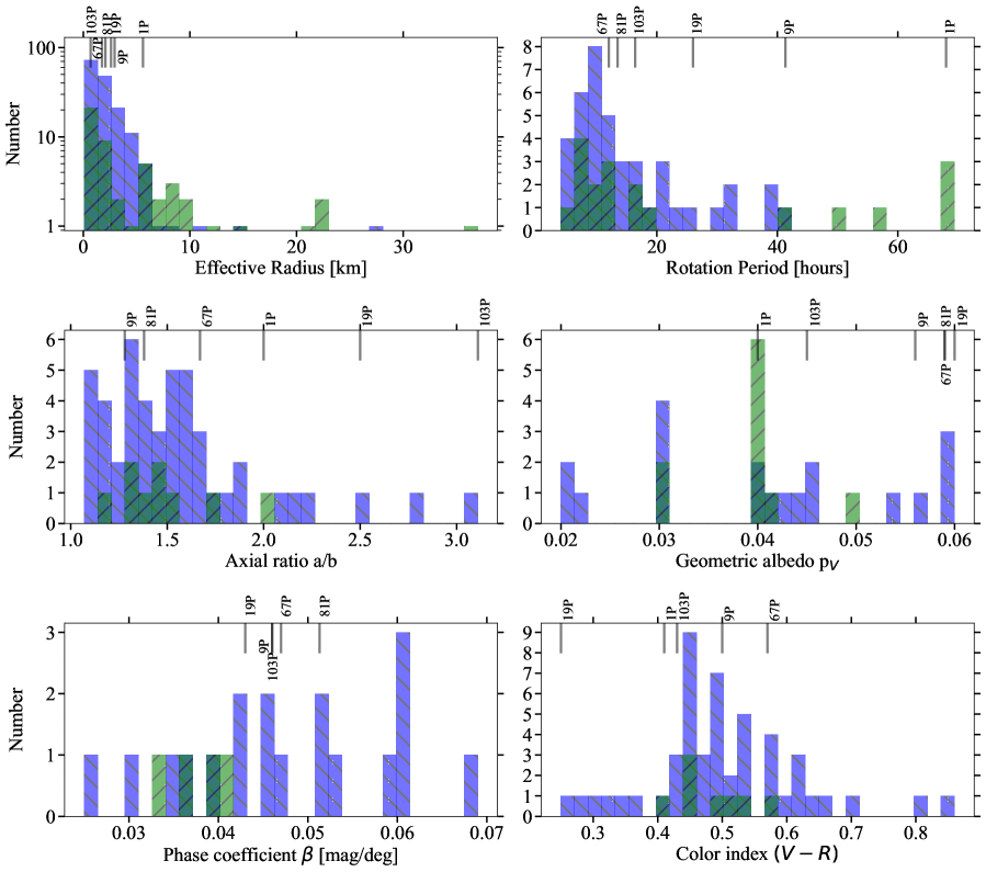
Figure 1: Histogram of the measured nucleus properties for JFCs (blue backward ($\backslash$) hashing) and HTCs plus LPCs (green forward (/) hashing). The values for comets with in-situ spacecraft measurements are indicated by vertical lines at the top axis. This figure aims to provide an overview of each parameter’s range and the sample size for which it has been measured. The property being plotted is given in the abscissa label for each plot. There are different numbers of comets in each sample because only a few comets have had all properties measured. As discussed in the text, the effective radius values are taken only from the thermal-IR studies of Fernández et al. (2013) and Bauer et al. (2017), while all other quantities represent our best effort to include all published values. In the cases when a comet had multiple measurements of a certain property, we have displayed the most recent sufficiently precise measurement, therefore only plotting a given comet’s property once. Note that most axial ratios plotted are lower limits. See the text for additional details.

3.1.2 Size-Frequency Distribution

Collecting the $r_{\mathrm{n}}$ of a large sample of objects and studying their cumulative size-frequency distribution (SFD) provides an invaluable tool to probe the formation and subsequent evolution of comets. The SFDs of minor-planet populations in the solar system are expressed as a power law of the form:

$$N(>r_{\mathrm{n}})\propto r_{\mathrm{n}}^{-a},$$ (5)

where $N$ is the number of objects with radius larger than $r_{\mathrm{n}}$. According to analytical models, collisionally relaxed populations of self-similar bodies with identical physical parameters have a power-law SFD with $a=2.5$. (Dohnanyi, 1969). In contrast, a shallower slope, $a=2.04$ is predicted for collisionally relaxed populations of strengthless bodies (O’Brien and Greenberg, 2003). Observations of asteroids reveal that their SFD shows characteristic “breaks”, or changes in the slope of the power-law distribution, which can be used to probe the material strength and the population evolutionary processes (e.g., O’Brien and Greenberg, 2005; Bottke et al., 2005).

Traditionally comets are presumed to have had a very different evolutionary history than the asteroid belt (e.g., they are not expected to have reached a collisionally steady state). Moreover they undergo sublimation-driven mass loss which is expected to result in significant differences between the SFDs of cometary populations and their source populations. However, recent work reviewed in Weissman et al. (2020) and Morbidelli et al. (2021) suggests that the source population of comets and TNOs in the primordial trans-Neptunian disk may have evolved to reach collisional equilibrium prior to being dispersed. While the debate about this possibility remains open, some of the deciding evidence may come from a better understanding of the small-end of the SFD of today’s remnants from the primordial transplanetary disk and specifically from comets. It is therefore informative to examine the observational evidence on the SFDs of short- and long-period comets in an attempt to distinguish the signatures of recent activity-driven evolution from those of planetesimal formation and/or early collisional history.

Earlier attempts to derive the SFD of JFCs from optical observations resulted in slightly different slopes, $a$ (e.g., Lowry et al., 2003; Lamy et al., 2004; Meech et al., 2004; Tancredi et al., 2006; Weiler et al., 2011). This highlighted the need to assess the uncertainty of the power-law slope determination by assessing the contribution of the various assumptions of the size estimates (e.g., on the albedo, phase function and shape of the nucleus, as well as photometric uncertainty). This was addressed by Snodgrass et al. (2011) and yielded a SFD with $a=1.92~{}{\pm}~{}0.20$ for JFCs with $r_{\mathrm{n}}~{}{\geq}~{}1.25$ km. This result is comparable to the SFD slopes determined for JFCs from thermal-IR observations ($1.92~{}{\pm}~{}0.23$; Fernández et al., 2013); both are consistent with the expected slope for a collisionally relaxed population of strengthless bodies (O’Brien and Greenberg, 2003), though as just discussed, the implications of this are not yet settled.

These studies, however, did not take into account the observational biases influencing the SFD, the most prominent being the bias against detecting small comet nuclei. Bauer et al. (2017), therefore, performed careful debiasing of the NEOWISE comet size estimates and determined a slope $a=1.0~{}{\pm}~{}0.1$ for LPCs and a steeper slope, $a=2.3~{}{\pm}~{}0.2$, for JFCs. This analysis, however, has left a few prominent questions unresolved. Theory suggests that there is an under-abundance of sub-km comets (e.g., Samarasinha 2007; Jewitt 2021); it is important for future observations to determine whether there is a paucity of small JFCs and what it reveals about comet disruption and the primordial SFD of outer-solar system planetesimals (Fernández et al., 2013; Bauer et al., 2017). Other features, such as the small bump in the SFD of JFCs between 3 and 6 km (Fernández et al., 2013), also remain to be confirmed and explained in the context of planetesimal formation or sublimation evolution (Kokotanekova et al., 2018). For more details about these debates, we refer the reader to Bauer et al. in this volume where the details of the telescope surveys used to derive the comet SFD are covered and to Fraser et al. in this volume where the comet size distribution is discussed in the context of other outer solar system populations.

3.1.3 Nucleus Shapes

Three main observational techniques can be employed to study the shapes of comet nuclei: rotational lightcurves, radar observations, and spacecraft data. The least complex and most easily available are rotational lightcurves in which the nucleus signal dominates the flux in the photometric aperture. Lightcurves in which coma flux dominates yield fundamentally different information and are discussed in Section 3.3.

Observations that are frequent enough, ideally on the same night or over several consecutive nights, can be combined to create a lightcurve, in which the magnitude is plotted as a function of time or rotational phase (if known). Lower limits to the projected nucleus axial ratio can be determined from the the peak-to-trough amplitude (${\Delta}m=m_{\mathrm{min}}-m_{\mathrm{max}}$) as

$$\frac{a}{b}~{}{\geq}~{}10^{0.4(m_{\mathrm{min}}-m_{\mathrm{max}})}$$ (6)

where $a$ and $b$ are the semi-long and and semi-intermediate axes in a triaxial ellipsoid in simple rotation, and $m_{\mathrm{min}}$ and $m_{\mathrm{max}}$ are the magnitudes at lightcurve minimum and maximum, respectively.

Broadly available for a large number of comet nuclei, $\Delta m$ allows the study of a large sample of comets (e.g., Lamy et al., 2004) under the assumption that they are approximately triaxial ellipsoids. Kokotanekova et al. (2017) updated the sample of well-constrained JFC lightcurves and estimated a median axial ratio of $a/b=1.5$, in agreement with the previous estimate from Lamy et al. (2004). We show in Figure 1 an updated version that includes all known comet axial ratios; these are also tabulated in Table 1A. The known range extends from 1.07 to 3.11 for the elongated nucleus of comet 103P. The axial ratios tabulated in Table 1A have a mean of $1.55~{}{\pm}~{}0.40$ and a median of 1.45. Similar results are obtained when considering only JFCs versus HTCs plus LPCs.

It is important to keep in mind that the projected axial ratio derived from rotational lightcurves is just a lower limit unless the spin axis is normal to the observer’s line-of-sight. If the lightcurve is observed at an unfavorable geometry or when the nucleus is surrounded by an undetected coma, the actual nucleus elongation can be significantly underestimated. This limitation becomes evident when the axial ratios of comets observed in-situ by spacecraft are compared to the total population average. Most spacecraft targets have axial ratios ($\geq$1.5), with comets 103P and 19P reaching some of the largest $a/b$ of 3.1 and 2.5 (Figure 1).

Rotational lightcurves taken at a wide variety of different observing geometries can also be analysed using the convex lightcurve inversion (CLI) technique (Kaasalainen and Torppa, 2001; Kaasalainen et al., 2001). This technique has been successfully applied to produce shape models for thousands of asteroids (Durech et al., 2010); a few comets have thus far been modeled, including 67P (Lowry et al., 2012), 162P (Donaldson et al., 2023), and 323P/SOHO (Hui et al., 2022b), as well as Don Quixote (Mommert et al., 2020). This method is limited to producing convex shape models and cannot recreate the concavities now known to be characteristic for comet nuclei (see below). Despite this limitation, CLI can accurately determine the object’s pole orientation and axial ratio with great precision. Another challenge posed by this method is that it requires a lot of observing time on comparatively large ($>$2-m) telescopes, given the faintness of bare comet nuclei. Additionally, only a small number of comets are inactive at large portions of their orbits, limiting the possibility to probe different observing geometries. However, an increasing number of bare nuclei have well-observed rotational lightcurves collected mainly to study changes in their rotation rates (see Section 3.3 below). The addition of data from future all sky surveys (see Section 4) may enable the shapes of additional comets to be constrained. Moreover, large flat surfaces on the asteroid convex shape models can be used to infer the existence of concavities (Devogèle et al., 2015). Combined with large elongations, this could reveal more contact binaries among the known JFC population and has the potential to improve our understanding of the binary fraction among comet nuclei (see below).

In the rare occasions when a comet passes sufficiently close to the Earth, radar delay-Doppler imaging can be performed to constrain the shapes of comet nuclei (see Section 2.2). At the time of Harmon et al. (2004)’s writing, nine comets had Doppler-only detection with radar and none had delay-Doppler imaging. Thanks to technological improvements and a confluence of close approaching comets, at least eight now have delay-Doppler imaging of their nucleus: 300P/Catalina (Harmon et al., 2006), 73P/Schwassmann-Wachmann 3 fragments B & C (Nolan et al., 2006), 8P/Tuttle (Harmon et al., 2010), 103P (Harmon et al., 2011), 209P/LINEAR (Howell et al., 2014), P/2016 (BA14 PANSTARRS) (Naidu et al., 2016), and 45P/Honda-Mrkos-Pajdušáková (Lejoly and Howell, 2017). Doppler only detections since Harmon et al. (2004) include 252P, 289P/Blanpain, 41P/Tuttle-Giacobini-Kresák (Howell et al., 2017), and 46P/Wirtanen (Lejoly et al., 2019). As evidenced by these studies, high-resolution radar imaging is occasionally possible. In such cases, precise shape modeling can be achieved by combining radar observations with optical light-curve modeling (see Ostro et al., 2002).

Finally, owing to the space missions equipped with on-board cameras (see Snodgrass et al. in this volume) the shapes of six comets have been studied in great detail (1P, 9P, 19P, 67P, 81P, and 103P). Four were found to be highly elongated or potentially bi-lobed: 1P (Keller et al., 1986), 19P (Britt et al., 2004; Oberst et al., 2004), 103P (Thomas et al., 2013b), and 67P (Sierks et al., 2015). Additionally, radar observations of comet 8P were consistent with a contact binary shape (Harmon et al., 2010).

The progress in characterizing comet nucleus shapes in the last decade revealed a striking overabundance of highly-elongated/bilobate objects in comparison to other minor planets. The comparison with other populations is somewhat complicated by the different definitions used by the different communities. Works focusing on NEAs often use a strict contact binary definition which sets a limit on the components’ mass ratio and implies that the objects might have been separate in the past (see Benner et al., 2015). TNO studies, on the other hand, are now making the first steps in understanding the shapes of individual objects and use a less restrictive definition (e.g., Thirouin and Sheppard, 2019). It is nevertheless informative to outline the contrasting findings for the different populations. Out of the six comets visited by spacecraft, four are highly-elongated/bi-lobed. If 8P is also considered, this sample of well-constrained comet shapes contains more than two-thirds highly-elongated/bi-lobed shapes. In comparison, only 14% of the almost 200 radar-imaged NEAs are bilobate (Taylor and Margot, 2011; Benner et al., 2015). The large abundance of bilobate shapes cannot be traced to the centaur region where no contact binary has been identified (Peixinho et al., 2020), while the contact-binary fraction among TNOs is estimated as 10%–25% for cold classicals or up to 50% for Plutinos (Thirouin and Sheppard, 2018, 2019). However, recently Showalter et al. (2021) presented evidence that the contact-binary fraction in the Kuiper Belt can even be higher if the shapes and the directional distribution of the objects’ rotation poles are accounted for.

The unusually large abundance of highly-elongated/bi-lobate objects among comets, prompted a number of works to investigate which combination of the comet’s physical properties and/or evolutionary processes have led to the formation of a large number of contact binaries. This motivation was further enhanced by the finding that New Horizons’ target in the cold classical Kuiper Belt, Arrokoth, is also a contact binary (Stern et al., 2019). Arrokoth’s shape is consistent with formation by merger of a collapsed binary system (McKinnon et al., 2020). However, unlike Cold Classical KBOs, the progenitors of JFCs have undergone giant-planet encounters and possibly a significant collisional evolution (Morbidelli and Nesvorný, 2020) which have most likely destroyed any distant binary systems early on. Instead, the formation of bilobate comet nuclei is better explained by the re-accretion of material ejected from catastrophic collisions in the early solar system (Jutzi et al., 2017; Schwartz et al., 2018) or even from multiple fission and reconfiguration cycles (Hirabayashi et al., 2016). Alternatively, modeling work by Safrit et al. (2021) shows that bilobate shapes can also form after comet nuclei experience rotational disruption caused by sublimation-driven torques soon after the onset of activity (e.g. during the centaur phase). As shown by Zhao et al. (2021), Arrokoth and by extension other icy bodies too could have evolved their shapes through sublimation to produce objects with enhanced elongated shapes if the conditions were right. It is remarkable that these scenarios not only reproduce the highly-elongated/bilobate shapes of comet nuclei but can also preserve the cometary physical properties and volatile content (Schwartz et al., 2018).

3.2 Cumulative Surface Properties of the Comet Population

The merit in exploring the cumulative surface properties lies in its potential to reveal dependencies between the comets’ surface properties and the physical properties or orbital characteristics which could, in turn, shed light on cometary evolution. On the other hand, comparing the bulk properties of comet nuclei with other minor planet populations could be used to establish the dynamical and evolutionary links among the diverse small-body populations in the solar system.

3.2.1 Albedo

The energy balance on the surface of a comet can be described using several photometric properties. The most frequently constrained is the geometric albedo $p_{\lambda}$ for a given wavelength $\lambda$, defined as the ratio between the disk-integrated reflectance at opposition and that of a perfectly reflective flat disk with the same size. If the phase function of the object at wavelength $\lambda$ is denoted by $\Phi$_λ$(\alpha)$, where $\alpha$ is the phase angle, and observations cover a large phase-angle range (typically covering a phase angle range of 70^∘ and above, Verbiscer and Veverka 1988), its phase integral $q_{\lambda}$ can be derived from:

$$q_{\lambda}=2\int{\Phi_{\lambda}(\alpha)\sin(\alpha)d\alpha}.$$ (7)

In such cases, the spherical albedo at wavelength $\lambda$, $A_{\lambda}$ (sometimes referred to as the Bond albedo), can be calculated as

$$A_{\lambda}=p_{\lambda}q_{\lambda}.$$ (8)

Physically, this is the fraction of power of the incident radiation that is scattered back into space over all angles and wavelengths. See Hanner et al. (1981) for further discussion of terminology.

The phase integral has been constrained by in-situ spacecraft observations of five JFCs: 19P (Li et al., 2007b), 9P (Li et al., 2007a), 81P (Li et al., 2009), 103P (Li et al., 2013) and 67P (Ciarniello et al., 2015). Besides 81P which has an exceptionally low phase integral of 0.16, the other JFCs have small phase integrals in the range 0.2-0.3, similar to small low-albedo asteroids (Verbiscer et al., 2019).

As indicated by Equation 2, determination of reliable nucleus sizes requires knowledge of the geometric albedo. Albedo can be determined by coupling simultaneous observations of sunlight reflected by the nucleus with observations that depend on the nucleus size but not its ability to reflect sunlight (most commonly via thermal re-radiation in the mid-IR). The geometric albedo can be determined using ground- and space-based telescopes (see Lamy et al. 2004 for details) and therefore, the sample of comet nuclei with well-constrained albedo in the visible range is comparatively large. The geometric albedos of JFCs were most recently reviewed by Snodgrass et al. (2011) and Kokotanekova et al. (2017), while the HTCs and LPCs were last summarized in Lamy et al. (2004).

As seen in Table 1B and Figure 1, this sample of 29 comet nuclei (19 JFCs and 10 HTCs plus LPCs) contains $V$-band albedos ($p_{V}$) between 0.02 and 0.06. Even though the absolute range is small, albedos vary by a factor $\sim$3 from darkest to brightest. This distribution clearly identifies comets as some of the darkest objects in the solar system. The unweighted average albedo of the whole sample of comets is $0.040~{}\pm~{}0.011$ (median 0.040). Subdividing into JFCs or HTC/LPC yield virtually identical values. Thus, the common practice of assuming $p=0.04$ when albedo is unknown (cf. Lamy et al., 2004) continues to be reasonable. Since $p_{\lambda}~{}{\sim}~{}0.04$ and $q_{\lambda}~{}{\sim}~{}0.2-0.3$, this means that $A_{\lambda}~{}{\sim}~{}0.01$, and thus $\sim$99% of the incident solar energy is absorbed by the comet.

Interestingly, as pointed out by Kokotanekova et al. (2018), the objects with the largest geometric albedos are all comets with albedo estimates from spacecraft observations (9P, 19P, 67P, 81P). On the other hand, the darkest surfaces belong mostly to the largest (Fernandez et al., 2016; Kokotanekova et al., 2017) and to the least active comets whose nuclei are easiest to characterize with telescope observations (Kokotanekova et al., 2018). The latter result may be an observational selection effect since small and dark objects will be more difficult to discover, but the former almost certainly is not – spacecraft targets were primarily selected for orbital accessibility.

As compared to other populations, comet nuclei span a narrow range of geometric albedos. The average albedo of comet nuclei is comparable to that of C, D and P-type asteroids (Mainzer et al., 2011) but unlike the asteroids of the respective classes, the comet population lacks objects with larger albedos. The consistently low albedo of comet nuclei has been utilized as a criterion to distinguish extinct comets from asteroids in the ACO populations identified by using dynamical criteria (Fernández et al., 2001; Licandro et al., 2016). Centaurs and Scattered Disk objects, thought to be the progenitors of current short-period comets, contain objects with albedos as low as those of comet nuclei. However, the mean geometric albedo of these populations is somewhat higher (0.056 for centaurs and 0.057 for SDOs) and they contain objects with albedos of up to 0.25. The known high-albedo surfaces of centaurs and TNOs are also associated with redder colors (larger spectral slopes in the visible) and form the “bright red” surface type with $18<S^{\prime}<58$ %/100 nm ($S^{\prime}$ is the normalized reflectivity gradient; see Section 3.2.3), and albedo $>$0.06 that is thought to disappear with the onset of centaur activity (see Jewitt 2015). On the other hand the “dark grey” centaurs have albedos similar to these of Jupiter trojans and Hildas (Romanishin and Tegler, 2018) which has been interpreted as evidence of the common origins of these populations and consequently between comet nuclei, Jupiter trojans, and Hildas.

An interesting question that has been difficult to answer broadly from telescope observations is whether comet surfaces have large-scale albedo variations. Synchronous visible/IR lightcurves (e.g., 10P by A’Hearn et al., 1989) suggest there are not, but can only be accomplished for a small number of low activity nuclei. It was, however, possible to search for surface areas with different albedos on the comets visited by spacecraft. While the brightness variations on the surface of 19P have been found to be up to a factor of 2 (Buratti et al., 2004; Li et al., 2007b), they are thought to be caused by surface roughness variations rather than differences in the albedo. All other comets that have been measured have smaller albedo variations, ${\lesssim}16\%$; 81P (Li et al., 2009), 9P (Li et al., 2007a), 103P (Li et al., 2013), and 67P (Fornasier et al., 2015).

3.2.2 Phase Function and Phase Reddening

The observed spectrophotometric properties of a reflecting surface are known to change depending on the phase angle, $\alpha$, of the observations. The spectral slope (as a function of wavelength) increase with $\alpha$ is referred to as phase reddening while the phase darkening, or phase function, describes the decrease of an object’s brightness with increasing $\alpha$. Moreover, at small phase angles $\alpha\leq 10^{\circ}$, the phase function can undergo a sharp nonlinear increase, known as the opposition effect (e.g., Gehrels, 1956).

These patterns are characteristic for airless regolith surfaces of solar system bodies. They can be analysed using physically motivated photometric models which relate the reflectance changes with the varying geometry and the properties of the object’s surface layer. The currently most widely used models follow the Hapke formalism (e.g., Hapke, 1981) and provide an opportunity to characterize the surface properties on small scales below the resolution of the observing instruments available on telescopes and most spacecraft. For example, careful modeling of the opposition effect or of the phase function beyond 90^∘ can be used to derive properties of the surface regolith at small scales. The moderate angle phase function, on the other hand, can be used to study the surface roughness and topography (see Verbiscer et al., 2013). In many cases, however, remote telescope observations of minor planets provide insufficient coverage to constrain the analytic photometric models. Instead, the phase function is approximated by a simpler parametric formalism, such as the IAU HG phase function (Bowell et al., 1989) which generally works well for of asteroids.

The phase functions of comet nuclei present an observational challenge because they require relatively large telescopes that are able to detect the bare nuclei and a substantial amount of observing time in order to characterize the rotation rate and correct for rotational variability. Despite the diversity of comet orbits, in practice, all nucleus phase functions observed from the ground span a narrow phase angle range of less than 20^∘ (see Kokotanekova et al., 2018) with the exception of 2P ($2.5-177^{\circ}$; Fernández et al. 2000). None of the nucleus phase functions (reviewed in Lamy et al. 2004, Snodgrass et al. 2011, and Kokotanekova et al. 2017) provide evidence for the presence of an opposition effect and are in excellent agreement with linear phase function fits, hence its use in Equation 3. Note that a different, non-linear phase function is used to characterize coma dust (e.g., Schleicher-Marcus model; Schleicher and Bair 2011)..

In situ observations during the fly-by missions covered a broad phase-angle range, but were insufficient to model the phase function close to opposition (Li et al., 2007a, b, 2009, 2013). Rosetta’s rendezvous with 67P was the first opportunity to observe a comet nucleus close to opposition. Even though the phase function between 0.5^∘ and 12.5^∘ of 67P from ground-based observations was well described by a linear function with a coefficient ${\beta}=0.059~{}{\pm}~{}0.006$ (Lowry et al., 2012), the disc integrated phase function of 67P observed by OSIRIS between $1.3-54^{\circ}$ exhibited a strong opposition effect and was better characterized by an IAU $HG$ model with $G=-0.13$ (Fornasier et al., 2015). The shape of the phase curve during the opposition effect derived from disk-resolved observations of different nucleus areas also enabled studies of the structure and properties of 67P’s surface (e.g., Masoumzadeh et al. 2017; Hasselmann et al. 2017).

Table 1B lists the phase coefficients of 24 comets (20 JFCs and 4 HTCs and LPCs) ranging from 0.025 to 0.07 mag/^∘. From this sample, the average phase coefficient for JFCs is $0.047~{}\pm~{}0.012$ mag/^∘ (with median 0.046 mag/^∘). As shown in Figure 1, the phase function slopes measured for LPCs and HTCs are smaller than the JFC average, though with the caveat that there are only five combined LPC plus HTC measurements. All phase coefficients determined from in-situ measurements, presumed to provide the most reliable estimates, are larger than the commonly used phase coefficient of 0.04 mag/^∘ (e.g. Lamy et al., 2004). We therefore recommend an updated value of 0.047 mag/^∘ to be assumed as an approximation when the phase coefficient of a nucleus is unknown.

Analyzing disk-resolved observations with VIRTIS, on-board Rosetta, Longobardo et al. (2017) found that terrains with larger roughness have steeper phase functions, At the same time a comparison with the phase functions from previous missions indicated that nuclei known to have rougher surfaces (81P and 9P) have steeper phase functions than 103P and 19P, characterized by smoother surfaces. Interestingly, dynamical studies of these five comets by Ip et al. (2016) suggested that the comets with smoother surfaces and shallower phase functions have spent more time in the inner solar system and have experienced more sublimation-driven erosion.

The notion that the phase functions of comet nuclei can reveal the extent of their surface evolution was strengthened when ground observations of JFC nuclei were included in the sample. Kokotanekova et al. (2017) identified a possible correlation of increasing phase coefficient with increasing albedo for the 14 JFCs with both of these parameters constrained (updated version shown in Figure 2). This was interpreted as a possible evolutionary path of JFCs where the least evolved comet nuclei have bright surfaces with steep phase possibly associated with volatile-rich surface layers and topography dominated by deep pits and cliffs (see Vincent et al., 2017; Kokotanekova et al., 2018; Vincent, 2019). This hypothesis suggests that sublimation-driven evolution is responsible for gradually eroding their surfaces which, in turn, decreases their albedos and phase coefficients. If confirmed by future observations, this idea provides a compelling possibility to characterize the evolutionary state of comets and to distinguish between extinct comets and objects of asteroidal origin (Kokotanekova et al., 2018). Alternatively, it is also conceivable that better phase-angle coverage and therefore better characterized nucleus phase functions in the future will challenge this hypothesis. For example, the phase coefficient of 162P was updated to a significantly larger value of 0.051 $\pm$ 0.002 mag/^∘ (Donaldson et al., 2023) which leads to a weaker Spearman rank correlation ($\rho=0.43$) as compared to the sample in Kokotanekova et al. (2018). Additionally, the smallest known JFC phase coefficient, that of 28P, is also likely to be much larger, $\sim$ 0.05mag/^∘ (Schleicher et al., 2022).

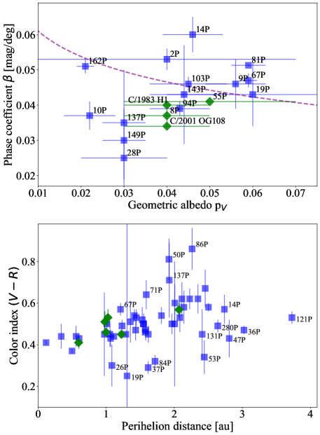
Figure 2: Plots of the two highest correlations we found in the datasets compiled here: phase coefficient as a function of geometric albedo (top panel) and $(V-R)$ color versus perihelion distance (bottom panel). The blue squares are JFCs and the green diamonds are HTCs and LPCs. The purple dashed line in the top panel is the correlation between phase coefficient and albedo for asteroids (Belskaya and Shevchenko, 2000). A recent update of 162P’s phase coefficient to a higher value has made the trend with albedo first identified in Kokotanekova et al. (2017) less pronounced. As identified by Lamy and Toth (2009) and discussed further in Section 3.2.3, there is a group of 10 comets that run parallel to, but below the main cluster in the color versus perihelion distance plot.

Nevertheless, it is interesting to note that asteroids follow a reverse correlation of decreasing phase coefficient for increasing geometric albedo (Belskaya and Shevchenko, 2000). However, their dataset does not allow conclusive results for objects with albedo similar to the darkest comet nuclei (smaller than 0.05). Another comparison between comet nuclei and asteroids worth considering is the presence of an opposition effect. The opposition effect amplitude (defined as the magnitude difference between the phase function at 0.3^∘ and the extrapolation of the linear part of the phase curve) is found to decrease for small albedos (Belskaya and Shevchenko, 2000). Moreover, some low-albedo Hilda asteroids and Jupiter trojans do not show evidence for the presence of an opposition effect down to very small phase angles (0.1^∘, Shevchenko et al. 2008). It is conjectured that the strong opposition effect found for 67P can be related to its comparatively large albedo. It is therefore essential to probe the phase functions of more comet nuclei of different albedos in order to verify how good of an approximation the linear phase function is.

Although attempts were made to determine the phase reddening of earlier fly-by mission targets, they were not successful. The long duration of the Rosetta rendezvous allowed the first detections of phase-reddening of a nucleus in the visible and near-infrared range (Ciarniello et al., 2015; Fornasier et al., 2015). The spectral slopes at different phase angles were analyzed for both disk-integrated and disk-resolved data and show a significant phase reddening in the $1.3^{\circ}-54^{\circ}$ phase angle range (from spectral slope $S^{\prime}$ of 11%/(100 nm) to 16%/(100 nm); Fornasier et al. 2015). In addition to this, the phase reddening was observed to vary with the changing heliocentric distance, first decreasing toward perihelion and then increasing again in the outbound orbit (Fornasier et al., 2016), indicating a significant seasonal variability.

Although the opposition effect and phase reddening have not yet been detected in ground-based data, both may be feasible to detect in the coming era (Section 4), and future investigators should be mindful of the possibility when analyzing their data. As shown by recent findings, the spectrophotometric properties of comet nuclei can be used to probe not only the physical characteristics of the surface layers of comets but also their sublimation-driven evolution. This highlights the need for future photometric and spectroscopic observations of bare nuclei both at different geometries and heliocentric distances.

3.2.3 Color and Spectra

Provided that sufficiently sensitive instruments are used, spectroscopy is the most desirable means of characterizing the nucleus surface as, in principle, it can reveal both precise color determinations and the presence of any absorption features due to surface ice or minerals. This compelling possibility motivated the early comet nucleus spectroscopy study by Luu (1993) which, however, revealed mostly featureless spectra. The absence of absorption features in the visible and near-IR has been confirmed by all subsequent spectroscopic observations (previously reviewed by, e.g., Lamy et al. 2004; Kelley et al. 2017; Licandro et al. 2018). As a result, the normalized reflectivity gradient $S^{\prime}$ (% per 100 nm) defined by A’Hearn et al. (1984) is the most commonly used parameter to characterize nucleus spectra. For visible wavelengths, reflectance is often normalized to 1 at some reference wavelength, frequently chosen to be 550 nm.

Though less informative than spectroscopy, the color index is determined from photometry by measuring the bare nucleus brightness in two filters and subtracting the magnitude at the longer wavelength from the shorter, e.g., $V-R$. Since photometric techniques are generally more sensitive than spectroscopy, this allows the colors of fainter nuclei to be measured with the caveat that they risk contamination by emission lines if unrecognized coma is present. This technique has been used to obtain the color indices of a wide variety of comet nuclei, building statistically significant samples covering the different classes of comets. A direct expression provided in Luu and Jewitt (1990b) allows an easy conversion between $S^{\prime}$ and the color index in the corresponding wavelength range (e.g., $V-R$, $B-R$, $R-I$, $g-r$, etc.) and allows for comparison of the surface colors of comets observed with either spectroscopy or photometry to other solar system populations. An important confirmation of the utility of ground-based spectroscopy was the finding that the spectrum of 67P near aphelion (Tubiana et al., 2011) was consistent with the visible and near-IR spectrum from OSIRIS on-board Rosetta (Fornasier et al., 2015).

In the visible to near-IR, comet surface spectra have spectral gradients up to 20% per 1000 Å (see Campins et al. 2007; Jewitt 2002; Kelley et al. 2017). While some spectra have been classified as closer T- and X-type asteroids (DeMeo and Binzel, 2008), most comet spectra have been identified to be closest to those of the primitive D-type asteroids which have similar spectral slopes (9.1 $\pm$ 1.1 % per 1000 Å; Fitzsimmons et al. 1994; Fornasier et al. 2007) and to some moderately red centaurs and TNOs (Fornasier et al., 2009). In the near-IR, comet nuclei exhibit spectral diversity similar to that known for Jupiter trojan asteroids (Emery and Brown, 2003; Campins et al., 2007, and references therein). The similarity between comets and Jupiter trojans extends to further spectral features such as the 10-$\mu$m emission plateau attributed to a surface layer of fine dust (Kelley et al., 2017; Licandro et al., 2018) and has been used to investigate the possible dynamical links between short-period comets and Jupiter trojans proposed by dynamical studies (e.g., Morbidelli et al., 2005).

Since the existing comet surface spectra probe mainly weakly active or extinct comets (e.g. 28P, 49P, 162P, 249P/LINEAR, 364P/PANSTARRS, 196256 (2003 EH1), P/2006 HR30 Siding Spring), the spectra of these objects have been used to study the transition to dormancy. It is a notoriously difficult problem to distinguish inactive objects with a cometary origin in the outer solar system (ACOs) from asteroids using purely dynamical criteria (see Fernández et al. 2005 and Tancredi 2014). Probing the spectra of ACOs is therefore considered to provide important clues on understanding the differences between these populations (Licandro et al., 2018; Simion et al., 2021). Additionally, increasing numbers of so called “active asteroids” (objects on typically asteroidal orbits that exhibit cometary activity; cf. Hsieh, 2017) and short-period comets whose dynamics suggest an origin in the asteroid belt (Fernández and Sosa, 2015; Hsieh et al., 2020) are being discovered. Considering this complexity, attributing any observed spectral signatures to the objects’ origin and evolution can be enhanced if combined with dynamical studies. This approach was assumed in the recent work by Kareta et al. (2021) who compared the reflectance spectra of three different dormant comets and inactive solar system small body 2003 EH1 in an attempt to study the diversity among the spectra of dormant comets and objects identified as meteor shower sources.

Previously, the surface colors of comet nuclei were reviewed by Lamy et al. (2004), Lamy and Toth (2009), and Solontoi et al. (2012); we have updated these reviews with subsequently published colors in Table 1B and Figure 1. Jewitt (2015) calculated the average color indices $B-V$, $V-R$, $R-I$, and $B-R$, distinguishing between nucleus and coma observations of JFCs and LPCs, and comparing them to the different TNO populations, centaurs, Jupiter trojans, and damocloids. This study reinforced previous findings that the average colors of the coma of JFCs and LPCs and centaurs are indistinguishable from the nucleus colors within the uncertainties. Additionally, the comparison between the nucleus colors of JFCs, LPCs, damocloids, and trojans are indistinguishable within the uncertainties for each class (Jewitt, 2015).

One of the main motivations behind comparing the surface colors of comet nuclei with centaurs and TNOs is understanding the absence of the so called “ultrared” material on comet nuclei (Jewitt, 2002). While a significant fraction of centaurs and TNOs contain the very red surfaces of spectral slopes $S^{\prime}>25$% (Lacerda et al., 2014, and references therein) and $B-R>1.5$ (see Tegler et al., 2008; Peixinho et al., 2012; Fraser and Brown, 2012; Tegler et al., 2016; Wong and Brown, 2017) alongside more neutral surfaces, none of the observed comet nuclei exhibit such extreme surface colors (with an average $B-R$ of 1.22 $\pm$ 0.03 and 1.37 $\pm$ 0.08 for LPC and JFC nuclei, respectively; Jewitt 2015). According to Jewitt (2015), the disappearance of the ultrared matter coincides with a perihelion distance of $\sim$10 au where centaur activity is observed to begin and is hypothesized to be due to blanketing of the primordially red material by fallback material ejected during the onset of activity.

Despite the effort to link surface color to different orbital and nucleus properties (perihelion distance, inclination, nucleus size, and active fraction) of comets, no statistically significant correlations have been found to date (cf. Lamy and Toth, 2009; Jewitt, 2015). We investigated correlations between our expanded collection of nucleus properties and various dynamical parameters (perihelion distance, aphelion distance, semi-major axis, eccentricity, inclination, and $T_{\mathrm{J}}$). The only relationship evincing some correlation is color with perihelion distance (plotted in Figure 2), with bluer nuclei having smaller perihelion distances (and a coupled trend of higher eccentricity JFCs having bluer nuclei), mimicking the behavior seen in the asteroid belt (e.g., Gradie and Tedesco, 1982) and among near-Earth asteroids (e.g., Marchi et al., 2006). Previously noticed by Lamy and Toth (2009), this apparent trend is not statistically significant (Spearman rank 0.47 for JFCs or 0.44 for all comets in our sample). However, similarly to Lamy and Toth (2009), we identify two distinct groups in the $(V-R)$ versus $q$ distribution. The main group consisting of 39 JFCs. Considering only comets from this group, results in a Spearman rank of 0.8, suggestive of a moderate to high correlation. Notably, all HTCs from the table also agree with the observed trend while both LPCs have perihelia much larger than 3 au and do not follow the observed trend. The second group consists of 10 JFCs which are bluer than the other group and follow a similar pattern of increasing redness with increasing heliocentric distance. We hypothesize that the existence of the second group can be connected with recent orbital changes, but interpreting these results is beyond the scope of this chapter.

As discussed briefly at the beginning of Section 3, we found no statistically significant correlations between surface color and the geometric albedo or phase coefficient for the JFCs. Owing to the paucity of polarization data (see next subsection), its correlation with other surface properties remains unexplored. The above links should be explored further with the precise color determinations expected from all-sky surveys such as the Vera Rubin Observatory’s Legacy Survey of Space and Time (LSST).

3.2.4 Polarization

Polarimetry is the study of the degree of polarization of light. Light becomes polarized – its electromagnetic wave having a preferred plane of oscillation – by scattering off of particles. The degree of linear polarization can be easily calculated (see Kolokolova et al. 2004 for details), and its variation reveals information about the particles from which it scattered. The degree of linear polarization of airless solar system bodies changes with phase angle and wavelength, producing a phase-polarization curve with a negative branch between 0^∘ and 20^∘ and a positive branch for higher phase angles that peaks in the range $90-100^{\circ}$ (cf. Kolokolova et al., 2004). Characterizing the phase-polarization curve of comet nuclei is limited by the faintness and the narrow phase angle range when comets are sufficiently far from the Sun to be inactive. Although polarimetric observations of comets date to the early 1800s (reviewed by Kiselev et al. 2015), it has only been applied to comet nuclei since 2004.

The first polarization studies of a comet nucleus were by Jewitt (2004a) who studied 2P at phase angles of 22^∘ as well as 93–100^∘. Later, Boehnhardt et al. (2008) observed the coma-free nucleus of 2P between 2.7 and 2.1 au, constraining its linear phase-polarization curve between 4^∘ and 28^∘ in $R$ and $V$-band. In this range, the polarization in both bands increases linearly with increasing phase angle, suggesting an inversion angle $\leq$4^∘. Similar low values of the inversion angle are characteristic for F-type asteroids (Belskaya et al., 2005) and have been found for active asteroid 107P/Wilson-Harrington (see Belskaya et al., 2019) and main-belt comet 133P/Elst–Pizarro (Bagnulo et al., 2010).

Kuroda et al. (2015) observed the linear polarization of the highly anemic 209P at large phase angles from 92.2^∘ to 99.5^∘. This was possible because 209P was very weakly active even at heliocentric distance $\sim$1 au and the nucleus polarization could be determined separately from that of the coma. They found no significant difference in 209P’s $R$ and $J$-band polarization and estimated that maximum polarization $P_{\mathrm{max}}=30.8$% is reached around the phase angles of the observations. Interestingly, the phase angle at which maximum polarization occurs coincides with that of asteroids, but the value of the maximum polarization of 209P is significantly higher. Boehnhardt et al. (2008) and Kuroda et al. (2015) explored whether existing empirical phase-polarization relationships for asteroids can be applied to comet nuclei. This subject remains to be explored further when the polarization of more comet nuclei is characterized in detail.

3.3 Spin State

3.3.1 Overview and Explanation of Terminology

The spin state, or the rotational state, of a comet fully describes the rotational properties of the nucleus. In this chapter, we use the terms “spin state” and “rotational state” interchangeably. A comet could be in (a) the least rotational kinetic energy “simple rotation” around its maximum moment of inertia (the latter is physically identified with the short axis, or more precisely the principal short axis defined by the moment of inertia ellipsoid) or (b) in an excited rotational state. An “excited” rotational state, by definition, has more rotational kinetic energy for a given rotational angular momentum than the least energy state described earlier.

A simple (i.e., a principal-axis) rotation requires three independent parameters and an initial condition to uniquely define it (the rotation period, two parameters defining the direction of the rotational angular momentum vector such as RA and Dec, and the orientation of a reference longitude of the nucleus at a specific time). In theory, a simple rotation could represent a rotation around any one of the three principal axes. However, a simple rotation around the intermediate principal axis or that around the long principal axis is extremely rare and both can be changed due to mechanical damping of energy. Thus, in this chapter, the term “simple rotation” means the least kinetic energy rotation around the short principal axis. The observational techniques for identifying and analyzing properties of simple rotations are discussed in the review by Samarasinha et al. (2004) in Comets II and thus not repeated here.

Except for the Principal-Axis (PA) rotational states around the intermediate principal axis or the long principal axis, a rotationally excited nucleus undergoes three concurrent component rotations, of which two are dynamically coupled, and such a spin state is known as a Non-Principal-Axis (NPA) rotation. In general, these component rotations occur at rates that vary with time but are periodic and therefore they can be expressed by time-averaged periods (e.g., Landau and Lifshitz 1976).

To uniquely define an NPA spin state, one requires six independent parameters and two initial conditions. These specific parameters and other details of the NPA rotation are described in Comets II. The NPA rotational states are the most general spin states and PA spin states can be considered limiting cases. The vast majority of cometary nuclei are observationally determined to be PA rotators in the least energy state; however, it is likely that many of them might be in slightly excited NPA states and groundbased observations are not sensitive enough to detect them (such as 67P; Gutiérrez et al. 2016).

3.3.2 Detection of NPA Rotation

As remarked earlier, many cometary nuclei appear to be simple rotators. However, delving deeper into the characteristics of NPA rotation helps us comprehend the observations of cometary spin and spin evolution of comets coherently. As described in the previous subsection, an NPA spin state is extremely complicated. Now, consider the possible NPA states of a nucleus that is near, but not exactly prolate. This nuclear shape is considered since different space mission images show many cometary nuclei are like that; lightcurves of nuclei, too, provide additional supporting evidence for this prevalent shape. Such a nucleus, if only slightly excited, is likely to be in a Short Axis Mode (SAM) whereas a highly excited nucleus will be in a Long Axis Mode (LAM) NPA state. The SAM and LAM NPA states are described in detail in Samarasinha et al. (2004) of Comets II and see their Figure 1 for visualizations of the NPA rotations described here.

The near-prolate nucleus undergoing a SAM NPA rotation has its long axis (a) rotating around the rotational angular momentum vector at a time-averaged angle of 90°, (b) a roll back-and-forth motion around the long axis itself with a back-and-forth half-rolling angle between 0° and 90°, and (c) a low-amplitude (i.e., a few degree) nodding motion. For a distant observer, the resultant lightcurve would be similar to that of a simple rotator within the observational uncertainties. Furthermore, if coma morphology is due to source region(s) near the end of the long axis, the coma morphology too would mimic a simple rotation. Only if the source region is located on the waist of the nucleus and the half-rolling angle is $\gg$0°, might the coma morphology hint an NPA rotation.

Similarly, if the nucleus is in a LAM NPA state, the long axis has (a) a precessional motion around the rotational angular momentum vector and making an angle $<$90°, (b) a full rolling motion around itself, and (c) a low-amplitude (i.e., a few degree) nodding motion. Again, the lightcurve may not be distinguishable from a simple rotator nor would the coma morphology caused by a source region(s) near the end of the long axis indicate an NPA rotation. However, a source region on the waist of the nucleus could point to an NPA state.

These examples point to the difficulty that observers face in conclusively identifying NPA rotators, especially if the signal-to-noise of the data is not high or there are not extensive data from multiple observing geometries. It would not be surprising if future observations indicate that some comets which we now consider to be simple rotators are in NPA spin states, or if discrepancies are found between simple/NPA spin states for different observational techniques.

3.3.3 Observational Evidence for NPA Spin and Excitation into and Damping of NPA Spin

So far, only two comets – 1P (e.g., Schleicher et al. 1990; Belton et al. 1991; Samarasinha and A’Hearn 1991) and 103P (e.g., A’Hearn et al. 2011; Samarasinha et al. 2011; Knight and Schleicher 2011; Drahus et al. 2011) – have been definitively shown to be in NPA rotation from remote observations. In both cases, extensive observations were required, a necessity that makes NPA rotation difficult to conclusively establish. Rosetta observations of 67P demonstrated that it is also excited, albeit at a level too low to detect from Earth (Gutiérrez et al., 2016; Kramer et al., 2019). Several other suspected NPA rotators are indicated by ^b? in Table 1A. Possible NPA spin states were suggested to explain conflicting observations or observations which were deemed incompatible with simple rotations. Clearly additional observations and analyses are needed to confirm NPA states for these comets.

An NPA spin state has been proposed for active centaur 29P/Schwassmann-Wachmann 1 with component periods of the order of a day (Meech et al., 1993). However, recent modeling based on multiple disparate data sets suggest a much longer rotation period for that comet (e.g., Miles 2016a; Schambeau et al. 2017, 2019).

The fraction of periodic comets observed to be in NPA states is much smaller than what the theory suggests based on the timescale for rotation period change of a simple rotator, $\tau_{\mathrm{P}}$, due to outgassing torques (Samarasinha et al., 1986; Jewitt, 1997). This timescale is indeed a lower limit to the timescale for rotational excitation; it will also depend on the relative component moments of inertia of the nucleus and the components of the torque. The rotational excitation of a nucleus is a complicated process and Gutiérrez et al. (2003b) cite the following as a necessary (but not sufficient) condition for a nucleus to get rotationally excited and to remain that way.

$$\frac{N_{\mathrm{l}}}{N_{\mathrm{s}}}>\frac{(I_{\mathrm{s}}-I_{\mathrm{i}})}{(I_{\mathrm{i}}-I_{\mathrm{l}})}\frac{|\Omega_{\mathrm{s}}|}{|\Omega_{\mathrm{l}}|}$$ (9)

where $N$, $I$, and $\Omega$ represent torque, moment of inertia, and angular velocity of the nucleus, respectively whereas $\mathrm{l}$, $\mathrm{i}$, and $\mathrm{s}$ represent respective components along long, intermediate, and short principal axes. From this condition, it can be seen that as near-prolate nuclei have nearly equal $I_{\mathrm{s}}$ and $I_{\mathrm{i}}$, such nuclei are comparatively easy to excite. Also, slow rotators (i.e., small $\Omega_{\mathrm{s}}$) are easier to excite than fast rotators (i.e., large $\Omega_{\mathrm{s}}$) and the former have comparatively small rotational kinetic energies. An explanation is presented in Section 3.3.6 as to why small nuclei are comparatively easier to excite. The reader is referred to Gutiérrez et al. (2003b) for an in depth discussion on the process of rotational excitation.

Even among the periodic comet nuclei, which experience recurrent torques due to outgassing, only a very small fraction of comets are observed to be in NPA states. In addition to the observational biases against discovering NPA states discussed earlier, a nucleus may be prevented from being excited if the damping timescale is shorter than the excitation timescale. A flexible nucleus (e.g., rubble-pile like) will have shorter damping timescales and most comets are likely to be structurally flexible objects with low tensile strengths. The loss of mechanical energy of a non-rigid body in an excited spin state causes it to ultimately rotate around the maximum moment of inertia. The corresponding damping timescale, $\tau_{\mathrm{damp}}$, was derived by Burns and Safronov (1973) to be ${\tau}_{\mathrm{damp}}~{}{\propto}~{}r_{\mathrm{n}}^{-2}\Omega^{-3}$, where $r_{\mathrm{n}}$ is the effective nuclear radius and $\Omega$ is the effective angular velocity. An immediate conclusion is large comets that are fast rotators have comparatively short damping timescales and are thus less likely to be in NPA spin states. Samarasinha (2008) discusses difficulties associated with deriving accurate damping timescales primarily due to our poor understanding of the values for structural parameters of comets. For example, for a 1 km radius nucleus with an effective rotation period of 1 day, ${\tau}_{\mathrm{damp}}$ can easily vary from ${\sim}10^{4}$ to ${\sim}10^{10}$ years depending on the structural flexibility of the nucleus. Therefore, ${\tau}_{\mathrm{damp}}$ could be of the same order as the orbital period for a few km sized fast rotating nucleus that is extremely flexible. On the other hand, ${\tau}_{\mathrm{damp}}$ could be as large as the age of the Solar System if the nucleus is comparatively more rigid. As most nuclei appear to be simple rotators (or close to that), it is likely that this is another pointer to the low rigidness of cometary nuclei.

3.3.4 Range of Measured Rotation Periods

Among the rotational parameters that define the spin state of a comet, the rotation period of the nucleus is the parameter that has measurements for the largest number of comets, albeit a relatively small number when compared with the asteroids with known rotation periods. This paucity of data is primarily due to impediments caused by cometary comae when deriving nuclear lightcuves of comets close to us (see Section 2).

Rotation periods can be determined from rotational lightcurves, coma morphology, or radar. As the latter two techniques were described in Section 2, we only discuss lightcurves here. Ideally, the flux in the photometric aperture would be dominated by the nucleus, but techniques that measure the coma flux have been successful for some comets. Common techniques for determining the correct rotation period from a lightcurve include phase dispersion minimization (commonly called PDM; Stellingwerf 1978), Fourier transformations (e.g., Belton, 1990), and simply aligning the lightcurves by eye. When the correct rotation period has been identified, data phased to this period will have their features (peaks and troughs) from different rotation cycles aligned with each other. Although rotational lightcurves are ideally acquired close together in time so that the viewing geometry is nearly constant, recent work by Kokotanekova et al. (2017) has shown that bare nucleus data acquired at widely separated epochs can reliably be combined in some circumstances.

The range of measured rotation periods of unambiguous comets varies from approximately four hours to multiple days (see Table 1A and Figure 1). Clearly this distribution is affected by observational selection effects. For example, to confidently derive a particular rotation period, typically an observational window longer than the rotation period is required, and therefore, there is a bias against deriving long rotational periods. Similarly, groundbased lightcurve observations have a bias against detecting rotation periods which are multiples of diurnal observing windows (e.g., periods near 12 and 24 hours) since nearly the same portion of the lightcurve is seen from night to night at the same location. Rotation periods based on the repetition of coma morphology have a distinct disadvantage against detecting short rotation periods because of the higher likelihood of coma structures getting smeared. The smearing occurs when the spatial separation of repeating features is less than the image resolution. Short rotation periods and low outflow speeds (e.g., of dust when compared with that of gas) cause closely spaced repetitive features whereas large geocentric distances cause low spatial resolution images.

In addition, there are a number of observational biases against measuring accurate rotation periods. They include lightcurve observations with small amplitude variability, either because of the intrinsic nuclear shapes or due to the specific observing geometries (for a nucleus lightcurves) or due to the diurnal activity pattern (for a coma lightcurve), and difficulties associated with detecting periods of NPA rotations discussed in the previous subsection.

Finally, different observational techniques could yield different manifestations of nuclear rotation (e.g., a nuclear lightcurve indicating a double-peaked lightcurve vs. coma morphology showing a periodic coma structure originating from a particular location on the nucleus vs radar observations of the nucleus) and care must be made to accurately interpret them and provide a consistent picture.

3.3.5 A Comet Spin Barrier?

Figure 3 plots rotation period versus axial ratio. This can be used to derive a lower limit to the bulk density of the nucleus under the strength-less body assumption. Lowry and Weissman (2003) derived a lower limit to the density of $\sim$600 kg/m³ from such a plot – corresponds to a minimum rotation period near 6 hours (also see Weissman et al. 2004, Lamy et al. 2004, and Kokotanekova et al. 2017) – a value consistent with direct density measurements for comet 67P by the Rosetta mission (Jorda et al., 2016). A review by Groussin et al. (2019) found a mean bulk density of $480\pm 220$ kg/m³ from 20 published estimates using a variety of techniques (see also Guilbert-Lepoutre et al., in this volume). A lower limit to the density estimated from a plot such as that in Figure 3 is derived for an ensemble and is extremely sensitive to a small number of comets spinning at periods near their rotational breakup periods. Thus this estimate should be considered only as a gross ensemble property but not as a density estimate for a particular comet.

In contrast to this “minimum” rotation period of $\sim$6 hours mentioned above for comets, the corresponding spin barrier for comparatively-sized asteroids occur at $\sim$2.2 hours (Warner et al. 2009, also see Hu et al. 2021). For comparatively-sized Jupiter trojans the barrier occurs at $\sim$4 hours (Chang et al. 2021) due to their higher densities than those of comets.

As noted earlier, there is a slight correlation between period and axial ratio. We suspect that this is an observational bias, due to the difficulty in detecting both low amplitude lightcurves and long rotation periods. However, fast rotators could also be missed, regardless of amplitude, if observations are not frequent enough. Future analyses with more robust observational data, e.g., from LSST, should investigate this further, but observational biases should be accounted for prior to interpreting the results.

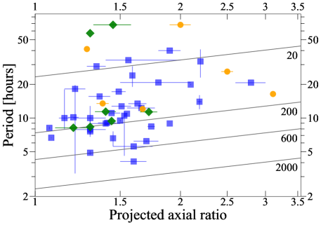
Figure 3: Rotation period against projected axial ratio for comet nuclei, updated from Kokotanekova et al. (2017). The blue squares are JFCs and the green diamonds are HTCs and LPCs. For these points, the axial ratio is a lower limit and the uncertainties are plotted when they were stated by the authors. When authors provided multiple equally likely periods, the shortest rotation period is plotted since this is most constraining. Orange circles are comets having shape models derived from spacecraft data. The diagonal lines indicate the minimum density (denoted in kg/m³ to the right), which a strength-less body of the given axial ratio and spin period requires to remain intact. Apart from the unusual case of 96P, which is undergoing continued fragmentation (Eisner et al., 2019) potentially related to rotational spin-up (see Section 3.4.3) no comet requires a density greater than $\sim$600 kg/m³ to remain stable against rotational breakup.

3.3.6 Evidence and Implications of Detected Rotation Period Changes

The idea that the rotation of comets could be altered by sublimation of gases dates back to the seminal work of Whipple (1950) in which he introduced the “icy conglomerate” model of the nucleus. In Whipple and Sekanina (1979), this concept was further expanded to examine how the torque caused by the jet force due to sublimation can result in the precession of the rotation axis of a non-rigid body nucleus rotating around its maximum moment of inertia. However, the actual situation could be much more complex. The net torque due to outgassing could cause rotational excitation to an NPA spin state as well as changes to its period(s) of rotation, in addition to the forced precession of the direction of the rotational angular momentum vector (e.g., Samarasinha et al. 2004 and references therein). As the rotation period has the largest spin parameter database including the most number of determinations on their temporal changes, we now concentrate on the current state of known rotation period changes.

Rotation period changes require precise measurements and typically (but not always) observations spanning multiple apparitions, making them challenging to determine. Just over a dozen have been measured or meaningfully constrained (see Table LABEL:tab:period_change), most since Comets II.

Samarasinha and Mueller (2013), based on four periodic comets, pointed out that the rotation period changes seem to be independent of the active fraction of a nucleus where active fraction is the fractional surface area of a solid water ice nucleus needed to reproduce the observed water production of the comet. They introduced a parameter $X$ given by

$$X=\frac{|\delta P|r_{\mathrm{n}}^{2}}{P^{2}\zeta}$$ (10)

where $P$ is the rotation period, $|\delta P|$ is the absolute value of the change of rotation period per orbit, $r_{\mathrm{n}}$ is the effective nuclear radius, and $\zeta$ is the total water production per unit surface area of the nucleus per orbit. It was found that $X$ was nearly constant for all comets despite a large scatter in the range of active fractions. They suggest highly active comets undergo more cancellation of torques. Mueller and Samarasinha (2018) added two more comets and found $X$ is still nearly constant. This near-constancy enables one to estimate $|\delta P|$ for various comets. Steckloff and Samarasinha (2018) proved that the sublimative torque model of Steckloff and Jacobson (2016) is consistent with the $X$ parameter model.

In Table LABEL:tab:period_change, $X$ is confined to approximately an order of magnitude and the geometrical mean of $\frac{X}{X_{\mathrm{E}}}$ of the 11 JFCs is $\sim$2 where $X_{\mathrm{E}}$ is the value of $X$ for comet 2P/Encke. The observations cover only portions of the active orbit instead of the entire active orbit for C/1990 K1 (Levy) (Schleicher et al., 1991; Feldman et al., 1992) and C/2001 K5 (Drahus and Waniak, 2006); for the latter, only the rate of spin change at the middle of the observing window is quoted (instead of the net change), so there is insufficient information for inclusion in Table LABEL:tab:period_change. Due to these reasons, we cannot properly estimate the $X$-parameters for these two comets. Upper limits exist for rotation period changes of three more JFCs – 14P/Wolf, 143P/Kowal-Mrkos, and 162P (Kokotanekova et al., 2018). However, as they do not meaningfully constrain the $X$-parameter, they are not listed in Table LABEL:tab:period_change.

Jewitt (2021) demonstrated that current observational data show that the active fraction, $f_{\mathrm{A}}$, and the effective dimensionless moment arm corresponding to sublimative torques, $k_{\mathrm{T}}$, approximately follow $f_{\mathrm{A}}\propto r_{\mathrm{n}}^{-2}$ and $k_{\mathrm{T}}\propto r_{\mathrm{n}}^{2}$ and therefore $f_{\mathrm{A}}k_{\mathrm{T}}$ is nearly constant. They also showed $f_{\mathrm{A}}k_{\mathrm{T}}$ is proportional to the $X$ parameter of Samarasinha and Mueller (2013). They argued these relationships for $f_{\mathrm{A}}$ and $k_{\mathrm{T}}$ are affected by significant observational biases and a debiased sample would make the $r_{\mathrm{n}}$ dependencies shallower for both $f_{\mathrm{A}}$ and $k_{\mathrm{T}}$. Therefore the net result would still be $f_{\mathrm{A}}k_{\mathrm{T}}$ (and therefore the $X$ parameter) is nearly constant.

The most direct conclusion from this spin evolution analysis is comets that have large active fractions show similar rotational evolution to comets with small active fractions. Comet nuclei have a range of active fractions spanning nearly three orders of magnitude (e.g., A’Hearn et al., 1995); the near-constant $X$ spans a factor of $\sim$500 in active fraction (Jewitt, 2021). The exceptions appear to be comets with very low active fractions (${\ll}0.1\%$), where the sublimative torques are apparently too weak to cause any spin evolution.

The rotation period change during an orbit is not necessarily a monotonic function of time (e.g., 9P; Belton et al. 2011; Chesley et al. 2013, 67P; Jorda et al. 2016; Kramer et al. 2019, 46P; Farnham et al. 2021b). So far, 46P is the most extreme case where rotation period changes during one segment of the orbit get cancelled during the subsequent segment of the orbit (see Farnham et al. 2021b) and this is likely due to the comet’s high obliquity of 70^∘ (Knight et al. 2021) as different torques dominate over different parts of the orbit. In fact, among the four comets whose intra-orbit spin changes are well-characterized, the percentage cancellation of $\delta P$ per orbit in increasing order are for comets 103P, 67P, 9P, and 46P. The obliquity (Table LABEL:tab:period_change) increases in order: 9P, 103P, 67P, and 46P; however, as 103P is an NPA rotator, its obliquity-induced seasonal effects will be moderated and presumably the cancellation of torques too. This hints at percentage cancellation of spin change during an orbit correlating with obliquity. Could nuclear shape also play a part in this? Additional observations during the coming decades may help answer this.

Table 2: Rotation Period Change per orbit ($\delta P$), effective nuclear radius ($r_{n}$), rotation period ($P$), total water production per unit surface area per orbit ($\zeta$), and $X$-parameter of comets (with respect to those of 2P/Encke, denoted by subscript $\mathrm{E}$) followed by the spin axis direction rounded to the nearest degree in (RA, Dec) and (orbital longitude, obliquity). In the row corresponding to 2P, the absolute values for 2P are given within parentheses in units of minutes, km, hours, kg m^-2, and m⁴ kg^-1s^-1, respectively. The orbital longitude is the angle measured prograde from the sun-perihelion direction in the orbital plane. The sense of rotation is not known for some spin axis directions and thus could be the diametrically opposite directions. The references are listed below the Table as footnotes.

					Spin Axis Direction
Comet	$\frac{|\delta P|}{|\delta P_{\mathrm{E}}|}$	$\frac{r_{\mathrm{n}}}{r_{\mathrm{nE}}}$	$\frac{P}{P_{\mathrm{E}}}$	$\frac{\zeta}{\zeta_{\mathrm{E}}}$	$\frac{X}{X_{\mathrm{E}}}$	RA (∘)	Dec (∘)	Orb Lon (∘)	Obliq (∘)
2P/Enckea,b	1	1	1	1	1	218	8	48	58
	(4)	(2.4)	(11)	(1.66$\times 10^{4}$)	(5.3$\times 10^{-5}$)
9P/Tempel 1a,c	3.5	1.18	3.73	0.35	1.0	255	64	285	16
10P/Tempel 2a,d	0.07	2.50	0.82	0.37	1.7	162	58	193	49
19P/Borrellya,e	$>$ 10	1.04	2.55	0.35	$>$ 4.8	214	-5	146	103
21P/Giacobini-Zinnerf	3.6, 6.3	0.42	0.86	0.43	1.9, 3.4	169	73	199	10
41P/Tuttle-Giacobini-Kresákg	390	0.29	3.2	0.46	7.0
46P/Wirtanenh	0.6, 3.0	0.25	0.82	0.45	0.12, 0.62	319	-5	240	70
49P/Arend-Rigauxi	$<$0.06	1.92	1.2	0.34	$<$0.45
67P/Churyumov-Gerasimenkoa,j	5.3	0.69	1.09	0.38	5.5	70	64	21	52
96P/Machholz 1k	$<$0.54	1.42	0.37	1.67	$<$4.8
103P/Hartley 2a,l	37.5	0.24	1.64	0.43	1.9	8	54	340	48
C/1990 K1 (Levy)m	57		3.3	0.38

^aMueller and Samarasinha (2018); ^bWoodney et al. (2007); also Sekanina (1988); Festou and Barale (2000); ^cThomas et al. (2013a); ^dKnight et al. (2012); ^eFarnham and Cochran (2002); Schleicher et al. (2003); ^fThere are two solutions for the spin period change; Goldberg et al. (2023); ^gAs the change in rotation period is large, the mean value is considered for the calculations; The possibility of NPA spin is suggested for this comet (see text) and if that is the case, this $X$-parameter estimate is highly uncertain; Bodewits et al. (2018); Howell et al. (2018); Schleicher et al. (2019); Jewitt (2021); ^hThe first entry for $\frac{P}{P_{\mathrm{E}}}$ and $\frac{X}{X_{\mathrm{E}}}$ represent the net change per orbit and the second entry for those correspond to the difference between the maximum and minimum rotation periods during the orbit (see text); Farnham et al. (2021b); Knight et al. (2021); ⁱEisner et al. (2017); ^jPreusker et al. (2015); Jorda et al. (2016); ^kEisner et al. (2019); ^lThis comet is in an evolving NPA spin state and a representative average based on the observations during the 2010 apparition is chosen as the rotation period; Belton et al. (2013); Knight et al. (2015); ^mObservations cover only a segment of the active orbit ($\sim$1 month); Schleicher et al. (1991); Feldman et al. (1992).

The timescale for rotation period change for a simple rotator, $\tau_{\mathrm{P}}$, can be expressed by (see Samarasinha et al. 1986; Jewitt 2021)

$$\tau_{\mathrm{P}}=k\frac{\rho_{\mathrm{n}}r_{\mathrm{n}}^{2}}{k_{\mathrm{T}}f_{\mathrm{A}}P\zeta}$$ (11)

where $k$ is approximately a constant. Since $f_{\mathrm{A}}k_{\mathrm{T}}$ is nearly constant, $\tau_{\mathrm{P}}\propto r_{\mathrm{n}}^{2}$. Therefore, smaller nuclei will change their rotation periods more rapidly. As can be seen in Kokotanekova et al. (2017) and Mueller and Samarasinha (2018), shorter rotation periods are preferentially seen among the smaller nuclei. This is consistent with sublimation driven spin evolution being the primary cause of spin changes among comets. For short period comets, $\tau_{\mathrm{P}}$ is smaller than their dynamical lifetime and small nuclei in particular should have undergone extreme alterations to their spin sometimes causing potential splitting events. As a result, particularly for periodic comets, the spin we observe today is not primordial. However, for extremely large comets (e.g., $r_{\mathrm{n}}\gg$ 10 km) or for DNCs, the spin alterations during their lifetimes are much smaller and they may retain some residual evidence of the primordial distribution. This interpretation is also consistent with $\tau_{\mathrm{P}}\sim 10^{2}r_{\mathrm{n}}^{2}$ suggested by Jewitt (2021) for comets with perihelia around 1-2 au, where $r_{\mathrm{n}}$ is in km and $\tau_{\mathrm{P}}$ is in years.

The changes to spin states due to outgassing torques can result in either a net spin-up or spin-down during an orbit. The nuclei which undergo spin-down may ultimately undergo spin-up, i.e., they will spin-down to extremely long periods and then reverse course and start spinning-up. During this epoch near extremely long rotation periods (with minimal rotational kinetic energies), if the conditions for rotational excitation are satisfied (see Section 3.3.3 and Gutiérrez et al. 2003b), the torques can put the nucleus into an excited spin state and it starts to spin-up. As $\tau_{\mathrm{P}}\propto r_{\mathrm{n}}^{2}$, the spin-down process too (similar to spin-up) is more efficient for smaller nuclei. Consequently, the rotational excitation is also more likely for smaller nuclei. The spin-up of nuclei is likely to be a cause of splitting events and is discussed in Section 3.4.3.

As sublimation induced forces are the cause for the non-gravitational forces that change the orbits of comets, Rafikov (2018) investigated the likely changes in the rotation period with corresponding non-gravitational forces and suggested they are correlated. As sublimation is the primary driver for both the rotational and non-gravitational force induced orbital changes of comets, simultaneous modeling of both these motions may be used to derive better constrained bulk densities for comets than just using orbital changes. Rafikov further determined that the dimensionless lever arm responsible for torquing was small, with a typical value around 1%, implying that most outgassing induced torques cancel themselves. Jewitt (2021) arrived at a similar conclusion from order of magnitude estimates of spin-up timescales.

3.3.7 Orientation of Spin Axes and Their Changes

Typically, the term spin axis refers to the axis defined by the angular velocity. For a simple rotator, the spin axis of the body aligns with the direction of the rotational angular momentum vector. For an NPA rotator, the instantaneous spin axis is not fixed either in the body frame or in the inertial frame. In this chapter, as most comet nuclei are simple rotators, the term “spin axis” is used for simplicity; however, in the case of an NPA rotator, the discussion implicitly refers to the direction of the rotational angular momentum vector despite the usage of the term “spin axis”.

Other than by space missions to comets, the primary means of determining spin axes of comets is using (a) coma morphology observations taken preferentially at different observing geometries, and (b) multi-epoch observations of the bare-nucleus lightcurves corresponding to different observing geometries. Unlike for asteroids, such multi-epoch bare-nucleus lightcurves are difficult to carry out and expensive in terms of telescope time. Therefore, most spin axis orientations of comets determined to-date are via morphological observations; however, the lightcurve method may become practical for many more comets in the LSST era (see Section 4).

Initial morphology-based spin axis determinations were based on broadband continuum features in the coma representative of scattering of sunlight by dust grains (e.g., Sekanina 1991b; Samarasinha and Mueller 2002; Farnham and Cochran 2002; Schleicher et al. 2003; Schleicher and Woodney 2003). With the relatively widespread use of narrowband filters within the last 2-3 decades, using primarily the morphology of CN features in the coma, many investigators were able to derive spin axes orientations of multiple comets or place useful constraints (e.g., Farnham et al. 2007a; Woodney et al. 2007; Samarasinha et al. 2011; Bair et al. 2018; Knight et al. 2021).

As mentioned earlier (Section 3.3.6), Whipple and Sekanina (1979) argued that the spin axis of a non-rigid oblate nucleus would “precess” due to non-gravitational torques. Numerical simulations by Samarasinha (1997) point to evolution of the spin axis due to sublimative torques, irrespective of if the spin state is excited or not. The spin axis gradually evolves either towards the orbital direction of peak outgassing (typically near perihelion) or the one diametrically opposite to that. Such a configuration is comparatively stable since that will provide the least net torque over time in the inertial frame. Subsequent work by Neishtadt et al. (2002) using a highly idealized model obtained the same result as one of the main evolutionary paths for the spin axis. Therefore, statistically, more spin axis directions may tend to align closer to the major axis of the orbit. As the current database for spin axis directions of comets is sparse, only future observations (e.g., from the LSST era) could test this prediction.

3.3.8 Properties and Processes Associated with Spin

Spin studies provide insight into how spin is related to activity and other physical and structural parameters of the nucleus. The discussions above make it clear how activity drives the spin state changes; it is appropriate to note that the spin state, too, is responsible for determining the activity of a comet, the seasonal effects of outgassing caused by a specific spin state being a well-known example. As remarked earlier, since the timescale for rotation period change is larger for large nuclei (e.g., Jewitt, 2021), their spin changes are difficult to measure and there is an observational selection effect against detecting spin changes of large nuclei.

Spin studies also provide insights into the structural properties of the nucleus (see Figure 4). The existence of a potential spin barrier and the disruption of comet D/1993 F2 (Shoemaker-Levy 9) due to jovian tidal effects are consistent with low strengths for cometary nuclei (of the order of 10 Pa, about a million times weaker than water ice; Weissman et al. 2004). In addition, the paucity of NPA spin states is a pointer to highly flexible nuclei with short damping timescales. However, both these structural traits should be considered as ensemble properties rather than specific to a particular comet. Here, the “flexibility of the nucleus” is meant to suggest that it is not a “perfect” rigid body but consists of a cohesive amalgamation of quasi sub-units held together weakly. This flexibility of the nucleus is also consistent with the frequent splitting events observed in comets (see next section). Although the activity and other activity-caused effects (e.g., spin-up) could be the primary trigger responsible for most splitting events, the low tensile strengths of comets could facilitate effortless splitting.

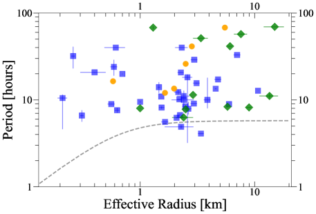
Figure 4: Rotation period against effective radius of comet nuclei, updated from Kokotanekova et al. (2017). The blue squares are JFCs, green diamonds are HTCs and LPCs, and orange circles are comets visited by spacecraft. The dashed line is the model for density 532 kg/m³, axial ratio 2, and tensile strength 15 Pa, which corresponds to the parameters measured for 67P from Rosetta (Groussin et al., 2015; Jorda et al., 2016). The two comets below the line are 61P, which also has two plausible longer period solutions (Lamy et al., 2011), and 96P, which is undergoing continued fragmentation (Eisner et al., 2019) potentially related to rotational spin-up (see Section 3.4.3).

It is possible that the cometary surface layer could be somewhat more cohesive and stronger than the interior but it is still weak when compared to water ice or even some forms of snow (see Guilbert-Lepoutre et al., in this volume). Naturally, it is likely that the low strengths for comets mean that the surface constituents (e.g., boulders) as well as the interior could respond to the stresses and resultant strains caused by rotation, including that due to NPA spin, by even altering cometary shapes. This possibility of mass redistribution and also the initiation of localized activity on the nucleus facilitated by a combination of low strengths of the nucleus and the rotation is an investigation worth pursuing in the future.

Spin state changes can cause cometary outbursts in at least two ways: (a) the spin-up-caused splitting can trigger outbursts due to exposure of new surface areas, and (b) the landslides triggered by rapid spin and/or spin changes can result in outbursts (Steckloff and Samarasinha (2018) and references therein). However, the majority of these outbursts are unlikely to be major contributors to changes in the spin state as the net torques due to outbursts are comparatively small (since most outbursts are of short duration).

3.4 Evolution of Physical Properties

Formation mechanisms and early evolution of comet nuclei are the focus of Simon et al. in this volume and were also the subject of excellent recent reviews by Dones et al. (2015) and Weissman et al. (2020). Briefly, the two leading formation theories are hierarchical agglomeration whereby smaller cometesimals gradually merge into larger bodies through low-velocity collisions with minimal influence of gravity (cf. Weidenschilling, 1997; Davidsson et al., 2016), and pebble accretion, in which mm- to cm-sized aggregates (“pebbles”) are formed out of dust and ice grains and then concentrated by the streaming instability until coalescing in a gravitational collapse (cf. Weidenschilling, 1977; Blum et al., 2017). Formation presumably occurred between 15 and 30 au (cf. Gomes et al., 2004), and the comets likely remained in this region for long enough that the population was significantly modified by collisional evolution (cf. Morbidelli and Rickman, 2015; Jutzi et al., 2017) before being scattered by giant planet migration to the Oort cloud or perturbed outwards into the Kuiper belt (e.g., the “Nice Model” Gomes et al., 2005; Tsiganis et al., 2005).

Once in these reservoirs, comets were likely further modified. As reviewed by Weissman et al. (2020), contributing processes are thought to include internal heating from short-lived radio-nuclides, heating by supernovae and passing stars, bombardment by high-energy particles, and accretion of and/or erosion by interstellar gas and dust grains. The first two processes would have heated nuclei at depth, affecting the volatile inventory and distribution. This has implications for the internal structure and composition (see chapters in this volume by Guilbert-Lepoutre et al. and Filacchione et al.). The last two processes are estimated to alter the top layers to perhaps 2 m (high-energy particles; see review by Strazzulla 1999) or $\lesssim$0.1 m (accretion/erosion; e.g., O’Dell, 1973; Stern, 1986). The above processes likely cannot appreciably change the size or shape of comet nuclei, though recent work by Zhao et al. (2021) suggests that sublimation could have significantly altered the shape of Arrokoth with additional assistance due to its specific spin orientation. The properties of the uppermost layers are undoubtedly altered by bombardment and accretion/erosion. This may result in changes to the color, albedo, phase function, and polarization, among other things. However, these are hard to discern observationally because the outermost layer is lost as soon as activity begins and typically before the comet is observable. These macroscopic surface properties could theoretically be measured in incoming dynamically new comets before significant activity has begun, but such observations are extraordinarily challenging (see Section 4).

Subsequent perturbation from the Kuiper belt or Oort cloud into smaller perihelion distance orbits will result in the initiation of activity (see the chapter by Fraser et al. in this volume). Changes in activity are likely gradual as comets diffuse inwards from the Kuiper belt and Scattered Disk via the centaur region into JFCs, or rapidly for Oort cloud comets, which can have their perihelion distance change by many au in a single orbit (Dybczyński and Królikowska, 2011). The more rapid perihelion changes of Oort cloud comets and corresponding dramatic increase in insolation may trigger some of the fragmentation scenarios discussed below. Activity removes material to a depth of order 1 m per orbit for a typical comet, although this is not necessarily uniform across the surface due to seasons, topography, and fallback. This is small compared to the size of typical comet nuclei, so it will not change the size or shape appreciably in a single orbit. However, the cumulative effects of activity-driven mass loss may modify the sizes and shapes of comet nuclei over their active lifetimes, which is likely of order 10³ to 10⁵ yr (e.g., Levison and Duncan, 1994, 1997) and dependent on both size and number of close perihelion passages (Nesvorný et al., 2017).

At the other end of their lifetimes, comets will be lost or destroyed by several mechanisms. Levison and Duncan (1997) estimate that the median dynamical lifetime of “ecliptic comets” (comets having $T_{J}>2$) is $4.5{\times}10^{7}$ years from the time of their first encounter with Neptune until they collide with the Sun or a planet, or are ejected from the solar system or into the Oort cloud. Thus, most comets will cease to be active long before they are ejected or destroyed by dynamical means. Inactivity may come about by loss of accessible volatiles or the formation of an inert crust; specific mechanisms and estimates of their timescales were reviewed by Jewitt (2004b) in Comets II. Such inactive comets could represent $\sim$10% of the near-Earth asteroid population (Fernández et al., 2001). See Jewitt and Hsieh, this volume, for additional discussion. Sub-km nuclei can be destroyed by mass loss due to sublimation alone (cf. Samarasinha, 2007). Fragmentation (or splitting) and disintegration are also common end states. The frequency of these events is not well constrained, but is estimated to be a few percent per orbit (e.g., Weissman, 1980; Chen and Jewitt, 1994). More than any other mechanisms just discussed, fragmentation has the potential to modify the nucleus properties discussed in the preceding subsections, so we explore it in more detail below.

3.4.1 Fragmentation Overview

The modern history of comet fragmentation begins with 3D/Biela, which was observed as a pair of fragments in 1846 following regular observations as a single nucleus since its discovery in 1772. It was recovered again in 1852 as a single comet, but has never been recovered since, with heightened meteor activity in 1872, 1885, 1892, and 1899 calculated to have originated in Biela’s orbit (see Kronk 1999, 2003 and references therein). High profile split comets in recent decades include Shoemaker-Levy 9, which was discovered as a string of nuclei in 1993 and subsequently observed to impact Jupiter in 1994 (cf. Hammel et al., 1995; Weaver et al., 1995), and 73P, which has had several apparently spontaneous fragmentation events since 1995 (cf. Sekanina, 2005) and whose fragments were observed in exquisite detail during a remarkable close approach to Earth in 2005 (e.g., Weaver et al., 2006; Reach et al., 2009). See Weissman (1980), Sekanina (1982), and Boehnhardt (2004) for lists of other split comets and more detailed discussion of their splitting scenarios.

Despite the relatively high frequency of comet splitting, only a few groups of dynamically related comets are known. Most of the persistent groups are near-Sun comets, almost exclusively seen only by solar observatories. Best known is the Kreutz sungrazing group (perihelion distance ${\sim}$0.005 au) which includes a number of historically bright, ground-observed comets including C/1882 R1 (Great September Comet) and C/1965 S1 (Ikeya-Seki) (cf. Marsden, 1967, 1989; Sekanina and Chodas, 2004), and thousands of minor fragments seen arriving in SOHO images every few days (cf. Biesecker et al., 2002; Knight et al., 2010). The minor fragments are seen only near the Sun for hours to days before they are destroyed, but are thought to have been produced by cascading fragmentation from one of a few major fragments since the previous perihelion passage (e.g., Sekanina, 2002). The Marsden and Kracht groups have ${\sim}10{\times}$ larger perihelion distances ($q~{}{\sim}~{}0.05$ au) and are thought to be descended from 96P/Machholz 1 as part of the “Machholz Complex” (Ohtsuka et al., 2003; Sekanina and Chodas, 2005). Little is known about the Meyer group, which also has much larger perihelion distances than the Kreutz group ($q~{}{\sim}~{}0.04$ au); it has not been linked to any other known objects but its members are thought to be on long period orbits. See Marsden (2005), Battams and Knight (2017), and Jones et al. (2018) for reviews of these near-Sun groups.

Few other groups of persistent families are known. Boehnhardt (2004) lists several likely split pairs/families, but uncertainties in orbital integrations, worsened by non-gravitational accelerations, make firm linkages difficult unless they are recently split; Tancredi (1995) estimated that even well known comet orbits cannot be integrated reliably for more than $\sim$1000 years. The only strong linkage of comets on typical JFC orbits seems to be 42P/Neujmin 3 and 53P/Van Biesbroeck (Carusi et al., 1985), while several likely split pairs of Oort cloud comets have been identified.

Most fragmentation events result in an initial brightening of the inner coma. As the new material expands, the inner coma brightness gradually returns to pre-outburst levels and one or more fragments may be discernible. There is generally a primary fragment having brightness approximately unchanged from before the event and fainter fragments which diminish in brightness or simply disappear on timescales of days to weeks. Frequently, but not always, the fainter fragments do not persist long enough to gain individual designations, and it is rare that they survive to be re-observed on subsequent apparitions. It is speculated (e.g., Jewitt, 2021) that these short lifetimes are due to rapid spin-up (see below), though other mechanisms such as rapid depletion of volatiles could also be responsible.

3.4.2 Outburst, Fragmentation, and Disintegration

Fragmentation may be part of a continuum of phenomena, including outbursts and disruption/disintegration (see Figure 5), that can modify the size, shape, and spin of a comet nucleus by progressively larger amounts. Most benign are outbursts, where a comet suddenly brightens due to a rapid, and usually short-lived, increase in activity. Historically, outbursts needed to be large to be detected (e.g., Ishiguro et al., 2016; Miles, 2016b) unless a comet was already under regular observation. However, with the improved cadences and depth of modern surveys, smaller outbursts are being discovered with much higher frequency than previously known. For instance, M. Kelley (U. of Maryland) and collaborators have reported outbursts of more than a dozen comets in Zwicky Transient Facility images since 2019 (e.g., Kelley et al., 2019; Lister et al., 2022). Deep Impact and Rosetta showed that outbursts too small to be detected from the ground happen frequently (Farnham et al., 2007b; Vincent et al., 2016), so it is reasonable to assume that the behavior is widespread. Belton (2010) proposed a taxonomy to explain a range of activity/outbursts of different strengths observed in spacecraft target comets.

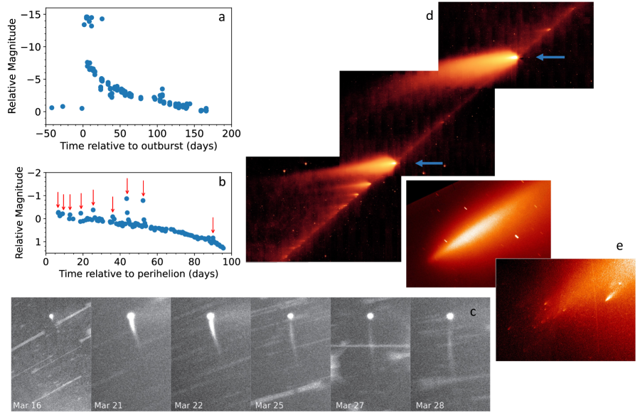
Figure 5: Examples of outbursts/fragmentation/disintegration. Panel a: Massive outburst of 17P/Holmes using selected “total” coma magnitudes archived with the Minor Planet Center. Time is measured from 2007 October 23.0. Panel b: Recurring minor outbursts of 7P/Pons-Winnecke adapted from Lister et al. (2022). Time is measured from perihelion (2021 May 27.1), and outbursts are indicated with vertical arrows. Panel c: Evolution of minor outburst morphology of 49P/Arend-Rigaux in 2012 from Eisner et al. (2017). Panel d: Extensive fragmentation of 73P/Schwassman-Wachmann 3 imaged 2006 May 4-6 by Spitzer. Persistent fragments are indicated with horizontal arrows. (Credit: NASA/JPL-Caltech/W. Reach (SSC/Caltech)) Panel e: Disintegration of C/1999 S4 (LINEAR) as seen on 2000 August 5. The lower right image by HST shows numerous discrete fragments that were not visible in the near-simultaneous upper left image acquired from the ground. (Credit: H. Weaver (the Johns Hopkins University), and the HST Comet LINEAR Investigation Team, University of Hawaii and NASA/ESA)

The largest outburst recorded is that of comet 17P/Holmes in 2007 where it brightened by nearly a million times just within two days (e.g., Montalto et al., 2008; Lin et al., 2009; Reach et al., 2010). However, except in the largest outbursts, the mass of material involved is likely very small compared to the whole nucleus. Estimates of the masses of the large outbursts reported in Ishiguro et al. (2016) are $10^{8}-10^{11}$ kg, considerably less than the ${\sim}10^{16}$ kg mass of 67P (Pätzold et al., 2019). For an assumed density of 600 kg/m³, a $10^{8}$ kg outburst corresponds to a sphere of equivalent radius $\sim$34 m. Thus, the volume of material involved in most outbursts is likely comparable to the sizes of the pits and boulders seen on 67P (e.g., Vincent et al., 2015; Pajola et al., 2016) and is insufficient, individually, to make appreciable changes in a comet’s size, shape, or rotation period.

Outbursts are occasionally accompanied by discrete brightness condensations in the coma which are identified as fragments. Fragments need not be associated with outbursts, and many are only discovered a considerable time after they were presumably produced. Identification of fragments and measurements of their sizes are limited by viewing geometry as well as the activity level of the coma. Graykowski and Jewitt (2021) identified fragments as small as 1 m in radius in HST observations of the debris field around the B and G fragments of 73P at 0.23 au from Earth in 2006, while the smallest discrete fragments identified by Weaver et al. (2001) of C/1994 S4 (LINEAR) at $\sim$0.7 au from Earth were $\sim$25 m in radius. We surmise that many outbursts which appear devoid of discrete fragments likely contain fragments either too small or too heavily enshrouded in coma to be detected.

Fragmentations can result in significant alteration of the original nucleus, particularly when the resulting pieces are large enough to persist. The primary surviving fragment of 73P is fragment C, which was estimated to have an equivalent radius of $\sim$0.5 km in 2006 (Toth et al., 2005; Graykowski and Jewitt, 2019) as compared to the pre-breakup radius of $\sim$1.1 km for the full comet (Boehnhardt et al., 1999). Sizes have not been published for the other fragments of 73P, but presuming they make up the bulk of the lost material, such mass loss could carry enough angular momentum and changes to the moments of inertia to significantly affect the rotation period and rotation state, in addition to the obvious changes to the size and shape.

The most extreme phenomenon in this continuum is disintegration, when the nucleus completely disappears. This may be accompanied by discrete fragments (e.g., C/1999 S4) or simply a diffuse cloud of material devoid of brightness condensations like C/2010 X1 (Elenin), in which no fragments were detected down to $\sim$40 m in radius (Li and Jewitt, 2015). Spontaneous disintegration seems to be far more common among dynamically new comets, an idea which we will revisit in the next subsection.

3.4.3 Causes of Fragmentation

A variety of mechanisms have been proposed to explain why comets split. In a few cases, the cause can be determined with some confidence, but most are conjecture. The most commonly accepted explanations for comet fragmentation are discussed below and illustrated in Figure 6.

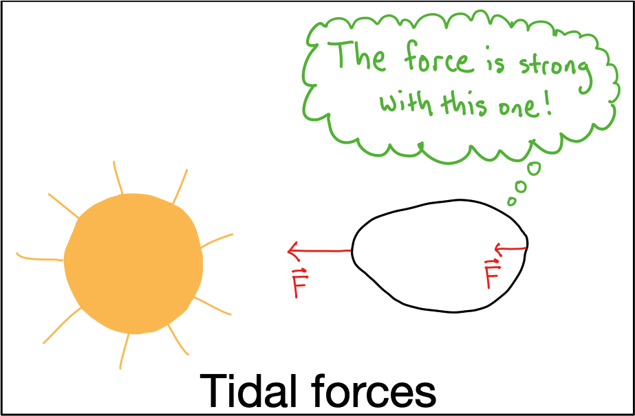
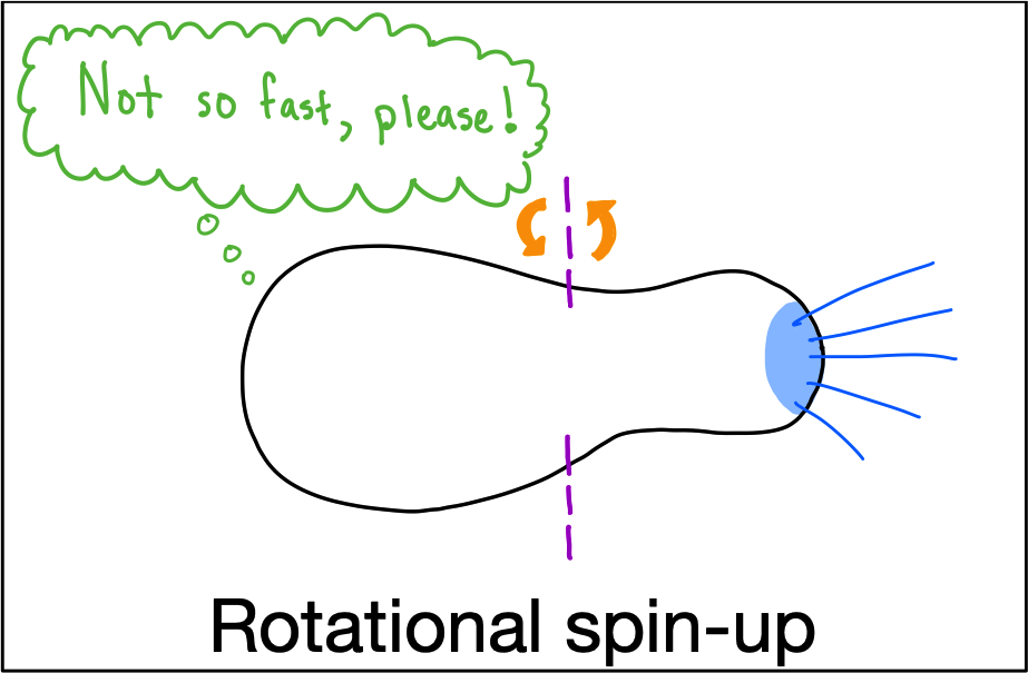
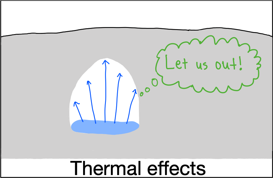
Figure 6: Causes of fragmentation (see text for additional details).

Tidal Forces — The differential gravitational force from a large mass felt on opposite sides of a less massive body can cause disruption of the latter if the differential gravitational force exceeds the forces acting to hold the body together. The splitting of sungrazing comets C/1882 R1 and Ikeya-Seki when near perihelion inspired Whipple (1963) and Opik (1966) to think of comet nuclei as (nearly) strength-less bodies, prone to split due to tidal forces based on their radius and density. The dramatic discovery of the string of fragments in Shoemaker-Levy 9 motivated a host of studies, which lead to the robust conclusion that it had been disrupted during a close approach to Jupiter in 1992 (e.g., Sekanina et al., 1994; Asphaug and Benz, 1996). Subsequent work has shown that the distance at which tidal splitting occurs can be modified to some extent by other properties of the nucleus such as the axial ratio, sense of rotation, and rotation period (see Knight and Walsh 2013 and references therein). However, such modifications are relatively small, and to first order, tidal splitting can be assumed to occur at the Roche limit.

Using the classical definition of the Roche limit as ${\approx}2.45~{}R_{\mathrm{p}}(\frac{{\rho}_{\mathrm{p}}}{{\rho}_{\mathrm{c}}})^{\frac{1}{3}}$, where $R_{\mathrm{p}}$ is the radius of the primary body, and ${\rho}_{\mathrm{p}}$ and ${\rho}_{\mathrm{c}}$ are the bulk densities of the primary and comet, a comet with a density of 600 kg/m³ is in danger of tidal splitting if it has perihelion within $\sim$3.2 solar radii (the common upper limit for orbits deemed to be “sungrazing”; see review by Jones et al. 2018), perijove within $\sim$3.2 Jovian radii, or perigee within $\sim$5.1 Earth radii. Encounters sufficiently close to induce tidal splitting are infrequent, with the only clear examples being several bright Kreutz sungrazing comets, Shoemaker-Levy 9, and 16P/Brooks 2 (Sekanina and Yeomans, 1985).

Rotational Spin-Up — A comet nucleus can split if the centrifugal forces due to rotation exceed the forces holding it together. As previously discussed, torques caused by the asymmetric outgassing of the nucleus can lead to changes in the rotation period and spin state. Although non-principal axis rotation states are known to exist, for simplicity, we consider the case of simple rotation here. Torques can act to either decrease (“spin-up”) or increase (“spin-down”) the rotation period. Spin-down decreases the centrifugal force and, thus, does not lead to splitting, while spin-up can lead to destruction, as has been discussed extensively in the literature, (e.g., Sekanina, 1982; Jewitt, 1997; Jorda and Gutiérrez, 2002).

As discussed in Section 3.3.6, smaller nuclei can spin up more rapidly than larger nuclei. Order of magnitude calculations (e.g., Jewitt, 2021) suggest that this can lead to catastrophic breakup of very small comet nuclei on surprisingly short timescales consistent with observations: 20–200 days at 1.6 au for 20 m radius fragments of 332P/Ikeya-Murakami (Jewitt et al., 2016) and $\sim$1.5 days at $\sim$0.06 au for 50 m radius sungrazing comets (Knight et al., 2010). Jewitt (2021) further argues that, for typical short-period comets of up to 10 km in radius, the timescale for destruction by spin-up is of order $10^{4}$ yr or less, and is shorter than the devolatilization timescale. Due, presumably, to the difficulty of making rotation period measurements for LPCs as well as no possibility of measuring a change in rotation period on subsequent orbits, only two Oort cloud comets have had a change in period detected, so a similar analysis cannot be conducted on the LPC population.

Even if these timescales are underestimated, observational evidence suggests spin-up is a frequent mechanism in the apparently spontaneous demise of comets. For example, size distributions of JFCs reveal an under-abundance of sub-km nuclei (e.g., Fernández et al., 2013; Bauer et al., 2017) that can be explained by spin-up, while Jewitt (2022) used a sample of 27 LPCs to argue that rotational breakup can explain the destruction of near-Sun long-period comets. However, note that spin-up is not necessarily the controlling factor in the destruction of small nuclei. As demonstrated by Jewitt (2021) and consistent with earlier work by Samarasinha (2007), either mass loss or spin-up can be the main driver of fragmentation.

A possibly related phenomenon is the disappearance of faint Oort cloud comets near the Sun. Bortle (1991) found that about 70% of Oort cloud comets for whom the absolute magnitude $H_{10}$ in the Vsekhsviatskii (1964) system was greater than $7.0+6.0q$, where $q$ is the perihelion distance in au, did not survive their perihelion passage. This equation is often referred to as the “Bortle limit.” Sekanina (2019) found even less frequent survival using a high quality set of modern orbits. On the assumption that fainter comets have smaller nuclei, this behavior can naturally be explained by sublimation driven spin-up, with increasingly larger nuclei being destroyed as perihelion distance decreases. In the most extreme case of a sungrazing comet, simulations by Samarasinha and Mueller (2013) predicted significant changes to the rotational state for C/2012 S1 (ISON) due to sublimation.

Thermal Effects — We use “thermal effects” to broadly encompass several processes related to the heating of the nucleus. The most commonly proposed mechanism is the buildup of subsurface gas pressure which is eventually released catastrophically as an outburst or fragmentation. A variety of processes have been proposed including the transition of amorphous to crystalline H₂O ice (e.g., Patashnick, 1974; Prialnik and Podolak, 1999) and exothermic dissolution of gases like CO and CO₂ (Miles, 2016b). Such processes are likely to be most important at large heliocentric distances; see reviews by Hughes 1991 and Gronkowski and Wesołowski 2016 for additional details. Thermal stress has often been cited as a likely cause of breakups (e.g., Boehnhardt, 2004). Fernández (2009) pointed out that the results from Deep Impact suggest that the thermal pulse from diurnal heating can only penetrate a few centimeters, so is unlikely to create large amounts of thermal stress.

Another thermal effect is the complete loss of the volatiles holding a comet together. As envisioned by Sekanina and Kracht (2018), a comet experiencing this might remain intact as a fluffy aggregate, but would be subject to extreme non-gravitational accelerations and would be expected to dissipate rapidly as the grains crumble. This loss of the volatile “glue” would be more likely to occur at small heliocentric distances and might, therefore, help explain the “Bortle limit” discussed above. In this scenario, there would be a survivor bias in which comets not prone to such behavior would survive, thus decreasing the frequency of disintegration by returning comets.

Shearing — The Rosetta team identified fractures that were centered in the neck region of 67P and propagated during the mission. Matonti et al. (2019) concluded that these expanding fractures were due to shearing deformation caused by stresses from 67P’s two lobes and speculated that this could cause outbursts at large distances or ultimately lead to 67P breaking up. Given the apparent prevalence of highly elongated/bilobate nuclei, this could be an important evolutionary mechanism across the comet population.

Impacts — Although collisional evolution of the comet population undoubtedly occurred in the early stages of the solar system, spatial densities throughout the solar system are too low for impacts onto comets to trigger fragmentation with any appreciable regularity today. However, small impacts undoubtedly occur on occasion, and may be capable of triggering increased activity by exposing fresh, subsurface ice.

3.4.4 Potential Insight Gained

Splitting provides the unique opportunity to study the freshly exposed interior of a nucleus. If each fragment is sufficiently separated spatially to allow its chemical composition to be measured, the compositions of fragments can be compared to investigate whether or not the parent nucleus was heterogeneous. To date, this has only been accomplished for 73P, whose fragments had similar compositions (e.g., Dello Russo et al., 2007; Schleicher and Bair, 2011). Measuring compositions of more split comets is highly desirable, as the results should help discriminate between nucleus formation scenarios, notably how bilobate nuclei come to be.

Rotationally resolved observations of recently split nuclei while they are weakly active or inactive would permit searches for color, albedo, and/or polarimetric variations. Since no comet has been shown to have appreciable macroscopic variations in any of these properties, the detection of variations in a recently split comet would suggest that fresh materials have different properties from older surface material.

If comets split along paths through their interiors with less structural integrity, the resulting more consolidated fragments may be the cometesimals out of which the original comet formed. It is interesting to note that the sizes of the fragments sampled in occasional high-resolution images of recent fragmentations – e.g., 73P, C/1999 S4, 332P (all discussed above) – are of similar sizes to the inferred sizes of the SOHO-observed Kreutz comets (Knight et al., 2010). Furthermore, all of these are consistent with Weidenschilling (1997)’s preferential sizes of cometesimals and roughly comparable in size to the boulders and pits on 67P (cf. Vincent et al., 2015; Pajola et al., 2016). If the fragments produced in splitting events are the fundamental units of comet formation, then measuring their size distribution will be valuable for constraining formation models. At present, the measured sizes of fragmented comets are thought to be limited by detector sensitivity. Future observations with greater survey depth should be capable of testing the small-end of this size distribution.

4 FUTURE ADVANCES

We conclude this chapter by considering what lies ahead for the study of comet nuclei. We limit this discussion to the discoveries that will advance the topics discussed in the preceding sections via remote observations. Future advances are obviously difficult to predict, but we shall make educated guesses based on the technological advances already underway or planned as well as well-established long term goals of the community. We supplement this with some wishful thinking if cost and/or luck were no impediment.

4.1 Near-term Telescope Advances

The easiest future insights to foresee are those that result from existing technology and soon-to-be completed facilities. The two major facilities expected to revolutionize planetary science in the near future are JWST and the Vera Rubin Observatory’s Legacy Survey of Space and Time (LSST).

4.1.1 JWST

JWST, a 6.5-m space-based telescope located at the Earth-Sun L2 Lagrange point, began operations in mid-2022 and is capable of acquiring images and spectra from 0.6 to 28.3 $\mu$m. Its unprecedented thermal IR capabilities provide fascinating possibilities for nucleus studies. Most known JFC nuclei should be detectable at aphelion, meaning that a dedicated survey could theoretically measure the nucleus sizes of essentially the entire JFC population. In reality, many are likely to be active at such distances (Kelley et al., 2013), making nucleus detections more challenging.

A more compelling advance would come from JWST detections of the nuclei of long period comets at large heliocentric distances post-perihelion, when activity has died down or is sufficiently low to allow the coma-nucleus separation techniques of Fernández et al. (2013). The efficiency is likely to be dependent on the dust-to-nucleus ratio, which would not be known in advance, but given the paucity of direct detections of the nuclei of comets coming from the Oort Cloud, would be well worth exploring. A study comparable in scope to SEPPCoN (Fernández et al., 2013) would have enormous value for shaping our understanding of the properties of LPC nuclei. Furthermore, JWST will enable surface spectroscopy of many more nuclei than have ever been studied in this manner. This may lead to the first remote detection of exposed ices and will make possible studies of spectral changes with rotation.

4.1.2 LSST

LSST is expected to begin full operations in early 2025. Surveying the entire sky visible from its southern hemisphere site in Chile every few nights to a limiting magnitude of $r{\approx}24.7$, LSST is predicted to increase the number of known comets by about an order of magnitude (Silsbee and Tremaine, 2016; Ivezić et al., 2019). Specific operational details are still being worked out and will have some effect on the number and nature of discoveries — a proposed twilight survey would find many new comets at small solar elongations (Seaman et al., 2018), while the proposed northern ecliptic survey would detect more distantly active bodies in the main asteroid belt, Kuiper belt, and (possibly) inner Oort cloud (Schwamb et al., 2018) — but it is clear that LSST will discover fainter and more distant objects than current surveys. The distant discoveries are especially enticing for the possibility of detecting bare nuclei of DNCs, allowing us to monitor the initiation of activity for the first time.

Most LSST discoveries will be too faint for detailed follow up, but the sheer number should vastly improve our understanding of the population of small and/or faint comets with large perihelion distances. The improved statistics should allow meaningful tests of population models (e.g., Silsbee and Tremaine, 2016). Frequent observations of individual comets may permit measurement of the physical properties of the nuclei of inactive or weakly active comets such as phase function, rotation period and axial ratios from lightcurves, color, and size for an assumed albedo. Regular monitoring will also allow the detection of unexpected activity or activity changes, both at individual epochs and by stacking multiple epochs. In addition to discovering many new weakly active comets, this will likely reveal many more fragmentation events than are currently known. The rapid identification of activity changes (e.g., Kelley et al., 2019) will enable the triggering of follow-up observations on specialized instruments that should yield even better data, such as size distributions of newly formed fragments.

4.2 Longer Term Telescope Advances

NEO Surveyor, the planned follow up to WISE/NEO-WISE, is slated to launch in 2026 and operate for at least 5 years (Sonnett et al., 2021). As proposed, it will have roughly 50% more collective power than WISE/NEOWISE and contain two passively cooled channels at mid-IR wavelengths, 4-5 $\mu$m and 6-10 $\mu$m. The longer wavelength channel should be virtually free of reflected sunlight, making it more effective than the post-cryogen phase NEOWISE at obtaining thermal measurements of comet nuclei. However, it will likely be less effective than the cryogen phase of the WISE mission, since the 4-5 $\mu$m region will suffer CO and CO₂ gas contamination, meaning the results will depend only on the longer wavelength channel (WISE had two gas-free bandpasses during its cryogen phase). On the whole, we expect NEO Surveyor to be capable of detecting the nuclei of smaller and more distant comets than WISE/NEOWISE, but to produce results that are more model dependent. NEO Surveyor’s much longer planned duration than the cryogen phase of WISE means it will detect many nuclei at multiple epochs; the repeat sampling should increase confidence in marginal results and may yield insight into the axial ratio of higher S/N targets.

A rebuilt Arecibo would reinstate our ability to directly measure nucleus properties of close-approaching comets. If it could be made more powerful, the volume of space in which such observations can be made greatly increases.

One or more 30-m class telescopes are expected to become operational by the late 2020s: the Extremely Large Telescope (39-m diameter in Chile), the Thirty Meter Telescope (30-m; Hawaii), and Giant Magellan Telescope (24.5-m; Chile). After JWST, the next major space-based observatory is expected to be the 2.4-m Nancy Grace Roman telescope with a launch date in the mid-2020s. Primarily planned to study dark energy and hunt for exoplanets, its primary value for comet studies is likely via serendipitous observations at large distances (Holler et al., 2021). The true successor to HST as a flexible, multi-wavelength space-based observatory is likely to be the Large Ultraviolet Optical Infrared Surveyor (LUVOIR). The LUVOIR concept is still being developed, but it is likely to have a 10-m class mirror and support imaging and spectroscopic capabilities from UV to IR wavelengths. Thirty meter class telescopes and next generation space telescopes will possess collecting power roughly an order of magnitude greater than the most powerful existing telescopes, thereby permitting detection and characterization of smaller and/or more distant nuclei. Those that overlap with the LSST era could enable detailed studies that are impossible with current technology. The high angular resolution of 30-m class telescopes could resolve nuclei of moderately sized comets without requiring extreme close approaches, might allow jets to be traced down to the active areas on the nucleus, or might detect sub-meter-scale fragments.

4.3 Serendipitous Advances

Advances that come from clever use of new technologies or simply luck are harder to predict. Entirely beyond our control are comets on orbits that bring them close enough to Earth for their nucleus properties to be measured. In general, encounters within 0.1 au yield outstanding data via numerous techniques. With diverse and often flexible missions in operation throughout the solar system, there are now more opportunities for close approaches of some kind than ever before. Indeed, the closest known approach of a comet to any planet was not a flyby of Earth, but C/2013 A1 (Siding Spring)’s 0.0009 au pass by Mars in October 2014 which yielded the first spatially resolved images of a dynamically new comet (Farnham et al., 2017).

Occultations are another opportunity that depend, to a great extent, on luck. To date, no comet nucleus has conclusively been detected by an occultation, though Fernández et al. (1999) constrained Hale-Bopp to ${\leq}$30 or ${\leq}48$ km depending on model parameters. The technique depends on measuring a shadow on Earth that is only the size of the occulting body, and whose position on Earth is uncertain in proportion to the positional uncertainty of the orbit and its distance from Earth. Comet occultations are more challenging than asteroids and even Kuiper belt objects due to their combination of small sizes, vastly larger positional uncertainty owing to their non-gravitational forces from outgassing, and optical depth effects. However, there is no technical reason preventing the observation of comet nucleus occultations. The highly successful campaign for New Horizons extended mission target Arrokoth (Buie et al., 2020), which correctly identified it as a contact binary and provided accurate estimates of the size of each lobe as well as the albedo, engenders optimism that a similar campaign could be mounted for the right comet. In principle, a relatively low cost program could be developed to attempt campaigns for promising targets. The logistics are daunting – tens to hundreds of observers spaced evenly across tens of km – but with persistence, chords across the nucleus of multiple long period comets might be obtained, unequivocally constraining their sizes at a fraction of the cost of a dedicated space mission.

Unexpected results from new technology provide another possible advance. A prime example of relevance to this chapter is the discovery in SOlar Heliospheric Observatory (SOHO) images that there exists a nearly continuous stream of small comets approaching the Sun. Small sungrazing comets belonging to the Kreutz family were known prior to SOHO (Marsden, 1989), but the discovery of thousands of such comets (cf. Battams and Knight, 2017) was unexpected, as was the existence of several other groups of dynamically related comets (Marsden, 2005). There is no facility currently planned that will rival SOHO’s surveying power, but the recently launched Parker Solar Probe (Fox et al., 2016) and Solar Orbiter (Müller et al., 2013), which are on trajectories with perihelion distance decreasing to 0.05 au and 0.28 au, respectively, might discover previously unknown groups of small comets near the Sun by fortuitously passing close to their orbits.

Moving further from luck to clever design, is the opportunity to use instrumentation in untraditional ways. JWST will allow parallel observations for many of its instruments. Parallel observations will have no control over telescope orientation, but careful planning for serendipitous pointing that include known comets or simply data mining to search for unknown objects might prove a low-cost way to explore comet nucleus properties. Data mining for serendipitous observations of known solar system objects has become relatively common (e.g., asteroids in Gaia data by Carry et al. 2021); similar work with JWST data could be particularly compelling if it can detect the nuclei of distant comets. Schlichting et al. (2012) constrained the size distribution of sub-km Kuiper belt objects by searching for occultations of stars in HST images; perhaps future work might be capable of probing the size distribution of the Oort cloud (e.g., Nihei et al., 2007; Ofek and Nakar, 2010)?

Finally, computationally intensive data mining of ongoing and future surveys will likely prove fruitful. Analyses that can combine many epochs of data at a multitude of possible rates of motion and then efficiently search the results may be capable of discovering much smaller and/or more distant comets than currently known. These will not only yield new discoveries, but could be used to determine many of the properties discussed in this chapter. The proliferation of stable, space-based datasets – Kepler/K2, TESS, GAIA – as well as deep ground-based surveys from larger telescopes like DECam on the Blanco 4-m at CTIO and Hypersuprime Cam on the 8-m Subaru telescope and, of course, LSST should provide ample input for such analyses over the next decade.

4.4 Open Questions

4.4.1 What is the range of comet nucleus properties?

As discussed previously, the size, axial ratio, albedo, color, phase slope, and rotation period have been measured for enough comet nuclei that we have a sense of their likely ranges. However, there are still few enough data points that individual measurements continue to have value in fleshing out the group statistics. A very reachable objective of the next decade or so is to measure each of these properties for enough comets to draw statistically significant conclusions, with the goal of making assessments akin to the revelation of the “spin barrier” among near-Earth asteroids (Pravec and Harris, 2000). Hints of this are already evident in the inference that comets had low densities prior to a direct measurement being made by Rosetta (Lowry and Weissman, 2003). However, might a clear limit be established for all comets, by dynamical class, or for a subset which share some common feature?

With sufficient data, exploration of the bounds of different properties might be especially insightful. Some questions which might be answerable in the relatively near future include: Is there a minimum size for comet nuclei? Is there a minimum and/or maximum albedo? What is the distribution of rotation periods? How common are highly-elongated/bilobate nuclei and what is their long-term stability if they outgas continuously? Are there binary nuclei similar to main-belt comet 288P (300163) (Agarwal et al., 2017)? Can phase function be used to discriminate between traditional asteroids and inactive comet nuclei on near-Earth object orbits?

4.4.2 What Are the Bulk Properties of the Nuclei of LPCs?

Tied closely to understanding the range of nucleus properties is the desire to understand the bulk properties of the comets originating from the Oort cloud. As discussed previously, few nucleus properties of LPCs are known, but a dedicated program to detect the nuclei of LPCs outbound at large heliocentric distances in the thermal IR with JWST may be capable of detecting sufficient numbers of LPC nuclei to determine bulk properties of this class of comets.

Another possibility is distant detections of inbound LPCs prior to the onset of activity. The recent discovery of comet C/2014 UN271 illustrates how challenging this will be. C/2014 UN271 was discovered in archival DECam images at $\sim$29 au (Bernardinelli et al., 2022). It is apparently exceptionally large and/or bright, so detection of a meaningful number of comets inbound requires being sensitive to smaller sizes. Since C/2014 UN271 was discovered at $V~{}{\approx}~{}22.5$, surveys would need to go to $V~{}{\approx}~{}27$, to detect 10 km objects at comparable distances. C/2014 UN271 exhibited clear activity in TESS data by a heliocentric distance of 23.8 au (Farnham et al., 2021a) and likely activity at $\sim$25 au in DECam images (Bernardinelli et al., 2021), so discoveries must be made at even larger distances if the nucleus is to be detected outright. Alternatively, discovering that only a small fraction of LPCs activate at large heliocentric distances would support the recently proposed lack of hypervolatile rich comets in the Oort cloud (Lisse et al., 2022).

Such observations might be feasible with one of the proposed 30-m class telescopes, though they would likely require a large field of view and dedicated time to survey a sufficiently large area of sky to get meaningful statistics about the population. This could be approached in a manner similar to the New Horizons team’s search for an extended mission target. Many epochs of deep imaging of the same fields eventually yielded the discovery of Arrokoth and compelling insights into physical properties of the faintest KBOs (Benecchi et al., 2015). Perhaps a 30-m class telescope “deep field” akin to the famous Hubble Deep field could achieve such a feat.

5 SUMMARY

Since the publication of Comets II, our knowledge of comet nucleus properties has grown considerably and a few hundred comet nuclei, dominated by JFCs but spanning across all dynamical types, have one or more physical and surface properties measured. The vast majority of this growth has come via remote observations. Several dedicated missions have provided ground-truth measurements and confirmed that remote observations can yield accurate measurements of bulk properties. Thus, it is becoming possible to use the cumulative nucleus properties to meaningfully constrain models of solar system formation and evolution. Highlights include:

• The effective radius has been measured or constrained for a few hundred comets. Most of these ($>$200) were included in two large-scale IR surveys whose data permit a debiased assessment of the size distribution.

• Ever improving observational capabilities and, in some instances, multi-orbit observations have yielded more than 50 axial ratio measurements and more than 60 rotation period measurements. In situ imaging from missions and radar observations have demonstrated that highly elongated and/or bilobate nuclei are common, motivating new investigations into how this might come to be.

• The number of comets with changes in rotation period measured or meaningfully constrained has increased from just one to about a dozen, leading to the surprising finding that rotation period changes seem to be nearly independent of the active fraction of the nucleus.

• The first nucleus polarization and delay-Doppler radar measurements have been made.

• Albedo and nucleus phase coefficients have each been measured for more than 20 comets, while nucleus color indices have been measured for more then 50 comets. A sufficient number of comets have had multiple nucleus surface properties measured to allow investigations into correlations between properties as well as comparisons with other small bodies in the solar system. When remote observations are combined with detailed mission data, studies into the “age” of comet surfaces are becoming viable.

• Detailed observations of several comets with highly favorable apparitions as well as greatly expanded surveying capabilities have led to advances in our understanding of nucleus spin states, outbursts, and disintegration/fragmentation.

We are on the cusp of the JWST and LSST eras that are expected to provide incredible new sources of data, potentially making every currently known JFC accessible and yielding direct detections of fainter and more distant comets than previously possible. These telescopes, along with several 30-m class ground-based facilities and eventual successors to HST and NEOWISE should enable the first widespread studies of Oort cloud comet nuclei and, undoubtedly, result in paradigm-shifting breakthroughs in our understanding of small bodies in the solar system.

Acknowledgments.

MMK acknowledges support from NASA Solar System Observations program grant NNX17AK15G / 80HQTR20T-0060. RK acknowledges support through the ESO Fellowship Programme. Funding via past NASA Planetary Science Division grants were instrumental in NHS’s contributions and this support is gratefully acknowledged. We thank Ellen Howell, Yan Fernandez, Michael S.P. Kelley, Abbie Donaldson, and Jian-Yang Li for helpful discussions.

References

- Abell et al. (2005) Abell P. A., Fernández Y. R., Pravec P. et al. (2005) Physical characteristics of Comet Nucleus C/2001 OG 108 (LONEOS), Icarus, 179, 174–194.
- Agarwal et al. (2017) Agarwal J., Jewitt D., Mutchler M. et al. (2017) A binary main-belt comet, Nature, 549, 357–359.
- A’Hearn et al. (2011) A’Hearn M. F., Belton M. J. S., Delamere W. A. et al. (2011) EPOXI at Comet Hartley 2, Science, 332, 1396–1400.
- A’Hearn et al. (1989) A’Hearn M. F., Campins H., Schleicher D. G. et al. (1989) The Nucleus of Comet P/Tempel 2, ApJ, 347, 1155.
- A’Hearn et al. (1986) A’Hearn M. F., Hoban S., Birch P. V. et al. (1986) Cyanogen Jets in Comet Halley, Nature, 324, 649–651.
- A’Hearn et al. (1995) A’Hearn M. F., Millis R. C., Schleicher D. O. et al. (1995) The ensemble properties of comets: Results from narrowband photometry of 85 comets, 1976-1992., Icarus, 118, 223–270.
- A’Hearn et al. (1984) A’Hearn M. F., Schleicher D. G., Millis R. L. et al. (1984) Comet Bowell 1980b, AJ, 89, 579–591.
- Anderson (2010) Anderson William Michael J. (2010) Infrared observations of oxidized carbon in comet C/2002 t7 (LINEAR), Ph.D. thesis, Catholic University, Washington DC.
- Asphaug and Benz (1996) Asphaug E. and Benz W. (1996) Size, Density, and Structure of Comet Shoemaker-Levy 9 Inferred from the Physics of Tidal Breakup, Icarus, 121, 225–248.
- Bach et al. (2017) Bach Y. P., Ishiguro M., and Usui F. (2017) Thermal Modeling of Comet-like Objects from AKARI Observation, AJ, 154, 202.
- Bagnulo et al. (2010) Bagnulo S., Tozzi G. P., Boehnhardt H. et al. (2010) Polarimetry and photometry of the peculiar main-belt object 7968 = 133P/Elst-Pizarro, A&A, 514, A99.
- Bair et al. (2018) Bair A. N., Schleicher D. G., and Knight M. M. (2018) Coma Morphology, Numerical Modeling, and Production Rates for Comet C/Lulin (2007 N3), AJ, 156, 159.
- Battams and Knight (2017) Battams K. and Knight M. M. (2017) SOHO comets: 20 years and 3000 objects later, Philosophical Transactions of the Royal Society of London Series A, 375, 20160257.
- Bauer et al. (2017) Bauer J. M., Grav T., Fernández Y. R. et al. (2017) Debiasing the NEOWISE Cryogenic Mission Comet Populations, AJ, 154, 53.
- Bauer et al. (2012) Bauer J. M., Kramer E., Mainzer A. K. et al. (2012) WISE/NEOWISE Preliminary Analysis and Highlights of the 67p/Churyumov-Gerasimenko near Nucleus Environs, ApJ, 758, 18.
- Bauer et al. (2011) Bauer J. M., Walker R. G., Mainzer A. K. et al. (2011) WISE/NEOWISE Observations of Comet 103P/Hartley 2, ApJ, 738, 171.
- Belskaya et al. (2019) Belskaya I., Cellino A., Levasseur-Regourd A.-C. et al. (2019) Optical Polarimetry of Small Solar System Bodies: From Asteroids to Debris Disks, vol. 460, p. 223.
- Belskaya and Shevchenko (2000) Belskaya I. N. and Shevchenko V. G. (2000) Opposition Effect of Asteroids, Icarus, 147, 94–105.
- Belskaya et al. (2005) Belskaya I. N., Shkuratov Y. G., Efimov Y. S. et al. (2005) The F-type asteroids with small inversion angles of polarization, Icarus, 178, 213–221.
- Belton (1990) Belton M. J. S. (1990) Rationalization of Comet Halley’s periods, Icarus, 86, 30–51.
- Belton (2010) Belton M. J. S. (2010) Cometary activity, active areas, and a mechanism for collimated outflows on 1P, 9P, 19P, and 81P, Icarus, 210, 881–897.
- Belton et al. (1991) Belton M. J. S., Julian W. H., Anderson A. J. et al. (1991) The spin state and homogeneity of comet Halley’s nucleus, Icarus, 93, 183–193.
- Belton et al. (2011) Belton M. J. S., Meech K. J., Chesley S. et al. (2011) Stardust-NExT, Deep Impact, and the accelerating spin of 9P/Tempel 1, Icarus, 213, 345–368.
- Belton et al. (2005) Belton M. J. S., Samarasinha N. H., Fernández Y. R. et al. (2005) The excited spin state of Comet 2P/Encke, Icarus, 175, 181–193.
- Belton et al. (2013) Belton M. J. S., Thomas P., Li J.-Y. et al. (2013) The complex spin state of 103P/Hartley 2: Kinematics and orientation in space, Icarus, 222, 595–609.
- Benecchi et al. (2015) Benecchi S. D., Noll K. S., Weaver H. A. et al. (2015) New Horizons: Long-range Kuiper Belt targets observed by the Hubble Space Telescope, Icarus, 246, 369–374.
- Benner et al. (2015) Benner L. A. M., Busch M. W., Giorgini J. D. et al. (2015) Radar Observations of Near-Earth and Main-Belt Asteroids, pp. 165–182.
- Bernardinelli et al. (2021) Bernardinelli P. H., Bernstein G. M., Montet B. T. et al. (2021) C/2014 UN271 (Bernardinelli-Bernstein): The Nearly Spherical Cow of Comets, ApJ, 921, L37.
- Bernardinelli et al. (2022) Bernardinelli P. H., Bernstein G. M., Sako M. et al. (2022) A Search of the Full Six Years of the Dark Energy Survey for Outer Solar System Objects, ApJS, 258, 41.
- Betzler et al. (2018) Betzler A. S., de Sousa O. F., and Betzler L. B. S. (2018) Photometric Study of Comet C/2014 S2 (PANSTARRS) After the Perihelion, Earth Moon and Planets, 122, 53–71.
- Betzler et al. (2020) Betzler A. S., de Sousa O. F., Diepvens A. et al. (2020) BVR photometry of comets 63P/Wild 1 and C/2012 K1 (PANSTARRS), Ap&SS, 365, 102.
- Biesecker et al. (2002) Biesecker D. A., Lamy P., St. Cyr O. C. et al. (2002) Sungrazing Comets Discovered with the SOHO/LASCO Coronagraphs 1996-1998, Icarus, 157, 323–348.
- Blum et al. (2017) Blum J., Gundlach B., Krause M. et al. (2017) Evidence for the formation of comet 67P/Churyumov-Gerasimenko through gravitational collapse of a bound clump of pebbles, MNRAS, 469, S755–S773.
- Bodewits et al. (2018) Bodewits D., Farnham T. L., Kelley M. S. P. et al. (2018) A rapid decrease in the rotation rate of comet 41P/Tuttle-Giacobini-Kresák, Nature, 553, 186–188.
- Boe et al. (2019) Boe B., Jedicke R., Meech K. J. et al. (2019) The orbit and size-frequency distribution of long period comets observed by Pan-STARRS1, Icarus, 333, 252–272.
- Boehnhardt (2004) Boehnhardt H. (2004) in Comets II (M. C. Festou, H. U. Keller, and H. A. Weaver, eds.), pp. 301–316, Univ. of Arizona Press/Lunar Planet. Inst., Tucson, AZ/Houston, TX.
- Boehnhardt et al. (2002) Boehnhardt H., Delahodde C., Sekiguchi T. et al. (2002) VLT observations of comet 46P/Wirtanen, A&A, 387, 1107–1113.
- Boehnhardt et al. (1999) Boehnhardt H., Rainer N., Birkle K. et al. (1999) The nuclei of comets 26P/Grigg-Skjellerup and 73P/Schwassmann-Wachmann 3, A&A, 341, 912–917.
- Boehnhardt et al. (2020) Boehnhardt H., Riffeser A., Ries C. et al. (2020) Mt. Wendelstein imaging of comet 41P/Tuttle-Giacobini-Kresak during the 2017 perihelion arc, A&A, 638, A8.
- Boehnhardt et al. (2008) Boehnhardt H., Tozzi G. P., Bagnulo S. et al. (2008) Photometry and polarimetry of the nucleus of comet 2P/Encke, A&A, 489, 1337–1343.
- Bortle (1991) Bortle J. E. (1991) Post-Perihelion Survival of Comets with Small q, International Comet Quarterly, 13, 89.
- Bottke et al. (2005) Bottke W. F., Durda D. D., Nesvorný D. et al. (2005) Linking the collisional history of the main asteroid belt to its dynamical excitation and depletion, Icarus, 179, 63–94.
- Bowell et al. (1989) Bowell E., Hapke B., Domingue D. et al. (1989) in Asteroids II (R. P. Binzel, T. Gehrels, and M. S. Matthews, eds.), pp. 524–556.
- Britt et al. (2004) Britt D. T., Boice D. C., Buratti B. J. et al. (2004) The morphology and surface processes of Comet 19/P Borrelly, Icarus, 167, 45–53.
- Buie et al. (2020) Buie M. W., Porter S. B., Tamblyn P. et al. (2020) Size and Shape Constraints of (486958) Arrokoth from Stellar Occultations, AJ, 159, 130.
- Buratti et al. (2004) Buratti B. J., Hicks M. D., Soderblom L. A. et al. (2004) Deep Space 1 photometry of the nucleus of Comet 19P/Borrelly, Icarus, 167, 16–29.
- Burns and Safronov (1973) Burns J. A. and Safronov V. S. (1973) Asteroid nutation angles, MNRAS, 165, 403.
- Campins et al. (1987) Campins H., A’Hearn M. F., and McFadden L.-A. (1987) The Bare Nucleus of Comet Neujmin 1, ApJ, 316, 847.
- Campins and Fernández (2002) Campins H. and Fernández Y. (2002) Observational Constraints On Surface Characteristics Of Comet Nuclei, Earth Moon and Planets, 89, 117–134.
- Campins et al. (2007) Campins H., Licandro J., Pinilla-Alonso N. et al. (2007) Nuclear Spectra of Comet 28P Neujmin 1, AJ, 134, 1626–1633.
- Campins et al. (1995) Campins H., Osip D. J., Rieke G. H. et al. (1995) Estimates of the radius and albedo of comet-asteroid transition object 4015 Wilson-Harrington based on infrared observations, Planet. Space Sci., 43, 733–736.
- Campins et al. (2006) Campins H., Ziffer J., Licandro J. et al. (2006) Nuclear Spectra of Comet 162P/Siding Spring (2004 TU12), AJ, 132, 1346–1353.
- Carry et al. (2021) Carry B., Thuillot W., Spoto F. et al. (2021) Potential asteroid discoveries by the ESA Gaia mission. Results from follow-up observations, A&A, 648, A96.
- Carusi et al. (1985) Carusi A., Kresák L., Perozzi E. et al. (1985) in IAU Colloq. 83: Dynamics of Comets: Their Origin and Evolution (A. Carusi and G. B. Valsecchi, eds.), vol. 115 of Astrophysics and Space Science Library, pp. 319–340.
- Carusi et al. (1987) Carusi A., Kresak L., Perozzi E. et al. (1987) High-Order Librations of Halley-Type Comets, A&A, 187, 899.
- Chang et al. (2021) Chang C.-K., Chen Y.-T., Fraser W. C. et al. (2021) FOSSIL. I. The Spin Rate Limit of Jupiter Trojans, \psj, 2, 191.
- Chen and Jewitt (1994) Chen J. and Jewitt D. (1994) On the Rate at Which Comets Split, Icarus, 108, 265–271.
- Chesley et al. (2013) Chesley S. R., Belton M. J. S., Carcich B. et al. (2013) An updated rotation model for Comet 9P/Tempel 1, Icarus, 222, 516–525.
- Ciarniello et al. (2015) Ciarniello M., Capaccioni F., Filacchione G. et al. (2015) Photometric properties of comet 67P/Churyumov-Gerasimenko from VIRTIS-M onboard Rosetta, A&A, 583, A31.
- Cruikshank et al. (1985) Cruikshank D. P., Hartmann W. K., and Tholen D. J. (1985) Colour, albedo and nucleus size of Halley’s comet, Nature, 315, 122–124.
- Davidsson and Gutiérrez (2006) Davidsson B. J. R. and Gutiérrez P. J. (2006) Non-gravitational force modeling of Comet 81P/Wild 2. I. A nucleus bulk density estimate, Icarus, 180, 224–242.
- Davidsson et al. (2016) Davidsson B. J. R., Sierks H., Güttler C. et al. (2016) The primordial nucleus of comet 67P/Churyumov-Gerasimenko, A&A, 592, A63.
- Delahodde et al. (2001) Delahodde C. E., Meech K. J., Hainaut O. R. et al. (2001) Detailed phase function of comet 28P/Neujmin 1, A&A, 376, 672–685.
- Dello Russo et al. (2007) Dello Russo N., Vervack R. J., Weaver H. A. et al. (2007) Compositional homogeneity in the fragmented comet 73P/Schwassmann-Wachmann 3, Nature, 448, 172–175.
- DeMeo and Binzel (2008) DeMeo F. and Binzel R. P. (2008) Comets in the near-Earth object population, Icarus, 194, 436–449.
- Devogèle et al. (2015) Devogèle M., Rivet J. P., Tanga P. et al. (2015) A method to search for large-scale concavities in asteroid shape models, MNRAS, 453, 2232–2240.
- Dohnanyi (1969) Dohnanyi J. S. (1969) Collisional Model of Asteroids and Their Debris, J. Geophys. Res., 74, 2531–2554.
- Donaldson et al. (2023) Donaldson A., Kokotanekova R., and Sondgrass C. (2023) The nucleus of 162P/Siding Spring from ground-based photometry, MNRAS.
- Dones et al. (2015) Dones L., Brasser R., Kaib N. et al. (2015) Origin and Evolution of the Cometary Reservoirs, Space Sci. Rev., 197, 191–269.
- Drahus et al. (2011) Drahus M., Jewitt D., Guilbert-Lepoutre A. et al. (2011) Rotation State of Comet 103P/Hartley 2 from Radio Spectroscopy at 1 mm, ApJ, 734, L4.
- Drahus and Waniak (2006) Drahus M. and Waniak W. (2006) Non-constant rotation period of Comet C/2001 K5 (LINEAR), Icarus, 185, 544–557.
- Durech et al. (2010) Durech J., Sidorin V., and Kaasalainen M. (2010) DAMIT: a database of asteroid models, A&A, 513, A46.
- Duxbury et al. (2004) Duxbury T. C., Newburn R. L., and Brownlee D. E. (2004) Comet 81P/Wild 2 size, shape, and orientation, Journal of Geophysical Research (Planets), 109, E12S02.
- Dybczyński and Królikowska (2011) Dybczyński P. A. and Królikowska M. (2011) Where do long-period comets come from? Moving through the Jupiter-Saturn barrier, MNRAS, 416, 51–69.
- Dybczyński and Królikowska (2015) Dybczyński P. A. and Królikowska M. (2015) Near-parabolic comets observed in 2006-2010 - II. Their past and future motion under the influence of the Galaxy field and known nearby stars, MNRAS, 448, 588–600.
- Eisner et al. (2017) Eisner N., Knight M. M., and Schleicher D. G. (2017) The Rotation and Other Properties of Comet 49P/Arend-Rigaux, 1984-2012, AJ, 154, 196.
- Eisner et al. (2019) Eisner N. L., Knight M. M., Snodgrass C. et al. (2019) Properties of the Bare Nucleus of Comet 96P/Machholz 1, AJ, 157, 186.
- Emery and Brown (2003) Emery J. P. and Brown R. H. (2003) Constraints on the surface composition of Trojan asteroids from near-infrared (0.8-4.0 m) spectroscopy, Icarus, 164, 104–121.
- Farnham et al. (2017) Farnham T., Kelley M. S., Bodewits D. et al. (2017) in AAS/Division for Planetary Sciences Meeting Abstracts #49, vol. 49 of AAS/Division for Planetary Sciences Meeting Abstracts, p. 403.01.
- Farnham (2009) Farnham T. L. (2009) Coma Morphology of Jupiter-Family Comets, Planet. Space Sci., 57, 1192–1217.
- Farnham and Cochran (2002) Farnham T. L. and Cochran A. L. (2002) A McDonald Observatory Study of Comet 19P/Borrelly: Placing the Deep Space 1 Observations into a Broader Context, Icarus, 160, 398–418.
- Farnham et al. (2021a) Farnham T. L., Kelley M. S. P., and Bauer J. M. (2021a) Early Activity in Comet C/2014 UN271 Bernardinelli-Bernstein as Observed by TESS, \psj, 2, 236.
- Farnham et al. (2021b) Farnham T. L., Knight M. M., Schleicher D. G. et al. (2021b) Narrowband Observations of Comet 46P/Wirtanen during Its Exceptional Apparition of 2018/19. I. Apparent Rotation Period and Outbursts, \psj, 2, 7.
- Farnham et al. (2007a) Farnham T. L., Samarasinha N. H., Mueller B. E. A. et al. (2007a) Cyanogen Jets and the Rotation State of Comet Machholz (C/2004 Q2), AJ, 133, 2001–2007.
- Farnham and Schleicher (2005) Farnham T. L. and Schleicher D. G. (2005) Physical and compositional studies of Comet 81P/Wild 2 at multiple apparitions, Icarus, 173, 533–558.
- Farnham et al. (2000) Farnham T. L., Schleicher D. G., and A’Hearn M. F. (2000) The HB Narrowband Comet Filters: Standard Stars and Calibrations, Icarus, 147, 180–204.
- Farnham et al. (2007b) Farnham T. L., Wellnitz D. D., Hampton D. L. et al. (2007b) Dust coma morphology in the Deep Impact images of Comet 9P/Tempel 1, Icarus, 187, 26–40.
- Feldman et al. (1992) Feldman P. D., Budzien S. A., Festou M. C. et al. (1992) Ultraviolet and visible variability of the coma of Comet Levy (1990c), Icarus, 95, 65–72.
- Feldman et al. (2004) Feldman P. D., Cochran A. L., and Combi M. R. (2004) in Comets II (Festou, M. C., Keller, H. U., & Weaver, H. A., ed.), pp. 425–447, University of Arizona Press, Tucson.
- Fernández and Sosa (2015) Fernández J. A. and Sosa A. (2015) Jupiter family comets in near-Earth orbits: Are some of them interlopers from the asteroid belt?, Planet. Space Sci., 118, 14–24.
- Fernández (2002) Fernández Y. R. (2002) The Nucleus of Comet Hale-Bopp (C/1995 O1): Size and Activity, Earth Moon and Planets, 89, 3–25.
- Fernández (2009) Fernández Y. R. (2009) That’s the way the comet crumbles: Splitting Jupiter-family comets, Planet. Space Sci., 57, 1218–1227.
- Fernández et al. (2006) Fernández Y. R., Campins H., Kassis M. et al. (2006) Comet 162P/Siding Spring: A Surprisingly Large Nucleus, AJ, 132, 1354–1360.
- Fernández et al. (2001) Fernández Y. R., Jewitt D. C., and Sheppard S. S. (2001) Low Albedos Among Extinct Comet Candidates, ApJ, 553, L197–L200.
- Fernández et al. (2005) Fernández Y. R., Jewitt D. C., and Sheppard S. S. (2005) Albedos of Asteroids in Comet-Like Orbits, AJ, 130, 308–318.
- Fernández et al. (2013) Fernández Y. R., Kelley M. S., Lamy P. L. et al. (2013) Thermal properties, sizes, and size distribution of Jupiter-family cometary nuclei, Icarus, 226, 1138–1170.
- Fernández et al. (2000) Fernández Y. R., Lisse C. M., Ulrich Käufl H. et al. (2000) Physical Properties of the Nucleus of Comet 2P/Encke, Icarus, 147, 145–160.
- Fernandez et al. (2016) Fernandez Y. R., Weaver H. A., Lisse C. M. et al. (2016) in American Astronomical Society Meeting Abstracts #227, vol. 227 of American Astronomical Society Meeting Abstracts, p. 141.22.
- Fernández et al. (1999) Fernández Y. R., Wellnitz D. D., Buie M. W. et al. (1999) The Inner Coma and Nucleus of Comet Hale-Bopp: Results from a Stellar Occultation, Icarus, 140, 205–220.
- Ferrín (2010) Ferrín I. (2010) Atlas of secular light curves of comets, Planet. Space Sci., 58, 365–391.
- Festou and Barale (2000) Festou M. C. and Barale O. (2000) The Asymmetric Coma of Comets. I. Asymmetric Outgassing from the Nucleus of Comet 2P/Encke, AJ, 119, 3119–3132.
- Fitzsimmons et al. (1994) Fitzsimmons A., Dahlgren M., Lagerkvist C. I. et al. (1994) A spectroscopic survey of D-type asteroids, A&A, 282, 634–642.
- Fitzsimmons and Williams (1994) Fitzsimmons A. and Williams I. P. (1994) The nucleus of comet P/Levy 1991 XI., A&A, 289, 304–310.
- Fomenkova et al. (1995) Fomenkova M. N., Jones B., Pina R. et al. (1995) Mid-Infrared Observations of the Nucleus and Dust of Comet P/Swift-Tuttle, AJ, 110, 1866.
- Fornasier et al. (2009) Fornasier S., Barucci M. A., de Bergh C. et al. (2009) Visible spectroscopy of the new ESO large programme on trans-Neptunian objects and Centaurs: final results, A&A, 508, 457–465.
- Fornasier et al. (2007) Fornasier S., Dotto E., Hainaut O. et al. (2007) Visible spectroscopic and photometric survey of Jupiter Trojans: Final results on dynamical families, Icarus, 190, 622–642.
- Fornasier et al. (2015) Fornasier S., Hasselmann P. H., Barucci M. A. et al. (2015) Spectrophotometric properties of the nucleus of comet 67P/Churyumov-Gerasimenko from the OSIRIS instrument onboard the ROSETTA spacecraft, A&A, 583, A30.
- Fornasier et al. (2016) Fornasier S., Mottola S., Keller H. U. et al. (2016) Rosetta’s comet 67P/Churyumov-Gerasimenko sheds its dusty mantle to reveal its icy nature, Science, 354, 1566–1570.
- Fox et al. (2016) Fox N. J., Velli M. C., Bale S. D. et al. (2016) The Solar Probe Plus Mission: Humanity’s First Visit to Our Star, Space Sci. Rev., 204, 7–48.
- Fraser and Brown (2012) Fraser W. C. and Brown M. E. (2012) The Hubble Wide Field Camera 3 Test of Surfaces in the Outer Solar System: The Compositional Classes of the Kuiper Belt, ApJ, 749, 33.
- Gehrels (1956) Gehrels T. (1956) Photometric Studies of Asteroids. V. The Light-Curve and Phase Function of 20 Massalia., ApJ, 123, 331.
- Gladman et al. (2008) Gladman B., Marsden B. G., and Vanlaerhoven C. (2008) Nomenclature in the Outer Solar System, p. 43.
- Goldberg et al. (2023) Goldberg C., Lejoly C., and Samarasinha N. (2023) Analysis of CN Coma Morphology Features of Comet 21P/Giacobini-Zinner, \psj, 4, 28.
- Gomes et al. (2005) Gomes R., Levison H. F., Tsiganis K. et al. (2005) Origin of the cataclysmic Late Heavy Bombardment period of the terrestrial planets, Nature, 435, 466–469.
- Gomes et al. (2004) Gomes R. S., Morbidelli A., and Levison H. F. (2004) Planetary migration in a planetesimal disk: why did Neptune stop at 30 AU?, Icarus, 170, 492–507.
- Gradie and Tedesco (1982) Gradie J. and Tedesco E. (1982) Compositional Structure of the Asteroid Belt, Science, 216, 1405–1407.
- Graykowski and Jewitt (2019) Graykowski A. and Jewitt D. (2019) Fragmented Comet 73P/Schwassmann-Wachmann 3, AJ, 158, 112.
- Graykowski and Jewitt (2021) Graykowski A. and Jewitt D. (2021) in AAS/Division for Planetary Sciences Meeting Abstracts, AAS/Division for Planetary Sciences Meeting Abstracts, p. 201.01D.
- Gronkowski and Wesołowski (2016) Gronkowski P. and Wesołowski M. (2016) A Review of Cometary Outbursts at Large Heliocentric Distances, Earth Moon and Planets, 119, 23–33.
- Groussin et al. (2019) Groussin O., Attree N., Brouet Y. et al. (2019) The Thermal, Mechanical, Structural, and Dielectric Properties of Cometary Nuclei After Rosetta, Space Sci. Rev., 215, 29.
- Groussin et al. (2015) Groussin O., Jorda L., Auger A. T. et al. (2015) Gravitational slopes, geomorphology, and material strengths of the nucleus of comet 67P/Churyumov-Gerasimenko from OSIRIS observations, A&A, 583, A32.
- Groussin et al. (2004) Groussin O., Lamy P., Jorda L. et al. (2004) The nuclei of comets 126P/IRAS and 103P/Hartley 2, A&A, 419, 375–383.
- Groussin et al. (2009) Groussin O., Lamy P., Toth I. et al. (2009) The size and thermal properties of the nucleus of Comet 22P/Kopff, Icarus, 199, 568–570.
- Groussin et al. (2010) Groussin O., Lamy P. L., and Jorda L. (2010) The nucleus of comet C/1983 H1 IRAS-Araki-Alcock, Planet. Space Sci., 58, 904–912.
- Gutiérrez et al. (2003a) Gutiérrez P. J., de León J., Jorda L. et al. (2003a) New spin period determination for comet 6P/d’Arrest, A&A, 407, L37–L40.
- Gutiérrez et al. (2016) Gutiérrez P. J., Jorda L., Gaskell R. W. et al. (2016) Possible interpretation of the precession of comet 67P/Churyumov-Gerasimenko, A&A, 590, A46.
- Gutiérrez et al. (2003b) Gutiérrez P. J., Jorda L., Ortiz J. L. et al. (2003b) Long-term simulations of the rotational state of small irregular cometary nuclei, A&A, 406, 1123–1133.
- Hainaut et al. (1998) Hainaut O. R., Meech K. J., Boehnhardt H. et al. (1998) Early recovery of Comet 55P/Tempel-Tuttle, A&A, 333, 746–752.
- Hammel et al. (1995) Hammel H. B., Beebe R. F., Ingersoll A. P. et al. (1995) HST Imaging of Atmospheric Phenomena Created by the Impact of Comet Shoemaker-Levy 9, Science, 267, 1288–1296.
- Hanner et al. (1981) Hanner M. S., Giese R. H., Weiss K. et al. (1981) On the definition of albedo and application to irregular particles, A&A, 104, 42–46.
- Hapke (1981) Hapke B. (1981) Bidirectional reflectance spectroscopy. I - Theory, J. Geophys. Res., 86, 3039–3054.
- Harmon et al. (1999) Harmon J. K., Campbell D. B., Ostro S. J. et al. (1999) Radar observations of comets, Planet. Space Sci., 47, 1409–1422.
- Harmon et al. (2010) Harmon J. K., Nolan M. C., Giorgini J. D. et al. (2010) Radar observations of 8P/Tuttle: A contact-binary comet, Icarus, 207, 499–502.
- Harmon et al. (2011) Harmon J. K., Nolan M. C., Howell E. S. et al. (2011) Radar Observations of Comet 103P/Hartley 2, ApJ, 734, L2.
- Harmon et al. (2006) Harmon J. K., Nolan M. C., Margot J. L. et al. (2006) Radar observations of Comet P/2005 JQ5 (Catalina), Icarus, 184, 285–288.
- Harmon et al. (2004) Harmon J. K., Nolan M. C., Ostro S. J. et al. (2004) in Comets II (M. C. Festou, H. U. Keller, and H. A. Weaver, eds.), pp. 265–280.
- Hasselmann et al. (2017) Hasselmann P. H., Barucci M. A., Fornasier S. et al. (2017) The opposition effect of 67P/Churyumov-Gerasimenko on post-perihelion Rosetta images, MNRAS, 469, S550–S567.
- Hicks and Bauer (2007) Hicks M. D. and Bauer J. M. (2007) P/2006 HR30 (Siding Spring): A Low-Activity Comet in Near-Earth Space, ApJ, 662, L47–L50.
- Hirabayashi et al. (2016) Hirabayashi M., Scheeres D. J., Chesley S. R. et al. (2016) Fission and reconfiguration of bilobate comets as revealed by 67P/Churyumov-Gerasimenko, Nature, 534, 352–355.
- Hoban et al. (1988) Hoban S., Samarasinha N. H., A’Hearn M. F. A. et al. (1988) An investigation into periodicities in the morphology of CN jets in comet P/Halley, A&A, 195, 331–337.
- Holler et al. (2021) Holler B., Milam S. N., Bauer J. M. et al. (2021) in Bulletin of the American Astronomical Society, vol. 53, p. 030.
- Holmberg et al. (2006) Holmberg J., Flynn C., and Portinari L. (2006) The colours of the Sun, MNRAS, 367, 449–453.
- Howell et al. (2018) Howell E., Belton M. J., Samarasinha N. H. et al. (2018) in AAS/Division for Planetary Sciences Meeting Abstracts #50, vol. 50 of AAS/Division for Planetary Sciences Meeting Abstracts, p. 106.06.
- Howell et al. (2017) Howell E. S., Lejoly C., Taylor P. A. et al. (2017) in AAS/Division for Planetary Sciences Meeting Abstracts #49, vol. 49 of AAS/Division for Planetary Sciences Meeting Abstracts, p. 414.24.
- Howell et al. (2014) Howell E. S., Nolan M. C., Taylor P. A. et al. (2014) in AAS/Division for Planetary Sciences Meeting Abstracts #46, vol. 46 of AAS/Division for Planetary Sciences Meeting Abstracts, p. 209.24.
- Hsieh (2017) Hsieh H. H. (2017) Asteroid-comet continuum objects in the solar system, Philosophical Transactions of the Royal Society of London Series A, 375, 20160259.
- Hsieh and Jewitt (2006) Hsieh H. H. and Jewitt D. (2006) A Population of Comets in the Main Asteroid Belt, Science, 312, 561–563.
- Hsieh et al. (2020) Hsieh H. H., Novaković B., Walsh K. J. et al. (2020) Potential Themis-family Asteroid Contribution to the Jupiter-family Comet Population, AJ, 159, 179.
- Hu et al. (2021) Hu S., Richardson D. C., Zhang Y. et al. (2021) Critical spin periods of sub-km-sized cohesive rubble-pile asteroids: dependences on material parameters, MNRAS, 502, 5277–5291.
- Hughes (1991) Hughes D. W. (1991) in IAU Colloq. 116: Comets in the post-Halley era (J. Newburn R. L., M. Neugebauer, and J. Rahe, eds.), vol. 167 of Astrophysics and Space Science Library, p. 825.
- Hui et al. (2022a) Hui M.-T., Jewitt D., Yu L.-L. et al. (2022a) Hubble Space Telescope Detection of the Nucleus of Comet C/2014 UN271 (Bernardinelli-Bernstein), ApJ, 929, L12.
- Hui and Li (2018) Hui M.-T. and Li J.-Y. (2018) Is the Cometary Nucleus-extraction Technique Reliable?, PASP, 130, 104501.
- Hui et al. (2022b) Hui M.-T., Tholen D. J., Kracht R. et al. (2022b) The Lingering Death of Periodic Near-Sun Comet 323P/SOHO, AJ, 164, 1.
- Ip et al. (2016) Ip W. H., Lai I. L., Lee J. C. et al. (2016) Physical properties and dynamical relation of the circular depressions on comet 67P/Churyumov-Gerasimenko, A&A, 591, A132.
- Ishiguro et al. (2016) Ishiguro M., Kuroda D., Hanayama H. et al. (2016) 2014-2015 Multiple Outbursts of 15P/Finlay, AJ, 152, 169.
- Ivanova et al. (2017) Ivanova O., Rosenbush V., Afanasiev V. et al. (2017) Polarimetry, photometry, and spectroscopy of comet C/2009 P1 (Garradd), Icarus, 284, 167–182.
- Ivezić et al. (2019) Ivezić Ž., Kahn S. M., Tyson J. A. et al. (2019) LSST: From Science Drivers to Reference Design and Anticipated Data Products, ApJ, 873, 111.
- Jehin et al. (2010) Jehin E., Manfroid J., Hutsemekers D. et al. (2010) Comet 103P/Hartley, Central Bureau Electronic Telegrams, 2589, 1.
- Jester et al. (2005) Jester S., Schneider D. P., Richards G. T. et al. (2005) The Sloan Digital Sky Survey View of the Palomar-Green Bright Quasar Survey, AJ, 130, 873–895.
- Jewitt (1997) Jewitt D. (1997) Cometary Rotation: an Overview, Earth Moon and Planets, 79, 35–53.
- Jewitt (2004a) Jewitt D. (2004a) Looking through the HIPPO: Nucleus and Dust in Comet 2P/Encke, AJ, 128, 3061–3069.
- Jewitt (2005) Jewitt D. (2005) A First Look at the Damocloids, AJ, 129, 530–538.
- Jewitt (2015) Jewitt D. (2015) Color Systematics of Comets and Related Bodies, AJ, 150, 201.
- Jewitt (2021) Jewitt D. (2021) Systematics and Consequences of Comet Nucleus Outgassing Torques, AJ, 161, 261.
- Jewitt (2022) Jewitt D. (2022) Destruction of Long-period Comets, AJ, 164, 158.
- Jewitt et al. (2015) Jewitt D., Hsieh H., and Agarwal J. (2015) The Active Asteroids, pp. 221–241.
- Jewitt and Luu (1989) Jewitt D. and Luu J. (1989) A CCD Portrait of Comet P/Tempel 2, AJ, 97, 1766.
- Jewitt et al. (2016) Jewitt D., Mutchler M., Weaver H. et al. (2016) Fragmentation Kinematics in Comet 332P/Ikeya-Murakami, ApJ, 829, L8.
- Jewitt and Sheppard (2004) Jewitt D. and Sheppard S. (2004) The Nucleus of Comet 48P/Johnson, AJ, 127, 1784–1790.
- Jewitt et al. (2003) Jewitt D., Sheppard S., and Fernández Y. (2003) 143P/Kowal-Mrkos and the Shapes of Cometary Nuclei, AJ, 125, 3366–3377.
- Jewitt (2002) Jewitt D. C. (2002) From Kuiper Belt Object to Cometary Nucleus: The Missing Ultrared Matter, AJ, 123, 1039–1049.
- Jewitt (2004b) Jewitt D. C. (2004b) in Comets II (M. C. Festou, H. U. Keller, and H. A. Weaver, eds.), p. 659.
- Jewitt and Meech (1988) Jewitt D. C. and Meech K. J. (1988) Optical Properties of Cometary Nuclei and a Preliminary Comparison with Asteroids, ApJ, 328, 974–986.
- Jones et al. (2018) Jones G. H., Knight M. M., Battams K. et al. (2018) The Science of Sungrazers, Sunskirters, and Other Near-Sun Comets, Space Sci. Rev., 214, 20.
- Jorda et al. (2016) Jorda L., Gaskell R., Capanna C. et al. (2016) The global shape, density and rotation of Comet 67P/Churyumov-Gerasimenko from preperihelion Rosetta/OSIRIS observations, Icarus, 277, 257–278.
- Jorda and Gutiérrez (2002) Jorda L. and Gutiérrez P. (2002) Rotational Properties of Cometary Nuclei, Earth Moon and Planets, 89, 135–160.
- Jorda et al. (2000) Jorda L., Lamy P., Groussin O. et al. (2000) in ISO Beyond Point Sources: Studies of Extended Infrared Emission (R. J. Laureijs, K. Leech, and M. F. Kessler, eds.), vol. 455 of ESA Special Publication, p. 61.
- Jutzi et al. (2017) Jutzi M., Benz W., Toliou A. et al. (2017) How primordial is the structure of comet 67P?. Combined collisional and dynamical models suggest a late formation, A&A, 597, A61.
- Kaasalainen and Torppa (2001) Kaasalainen M. and Torppa J. (2001) Optimization Methods for Asteroid Lightcurve Inversion. I. Shape Determination, Icarus, 153, 24–36.
- Kaasalainen et al. (2001) Kaasalainen M., Torppa J., and Muinonen K. (2001) Optimization Methods for Asteroid Lightcurve Inversion. II. The Complete Inverse Problem, Icarus, 153, 37–51.
- Kareta et al. (2021) Kareta T., Hergenrother C., Reddy V. et al. (2021) Surfaces of (Nearly) Dormant Comets and the Recent History of the Quadrantid Meteor Shower, \psj, 2, 31.
- Kareta et al. (2022) Kareta T., Reddy V., Sanchez J. A. et al. (2022) Near-infrared Spectroscopy of the Nucleus of Low-activity Comet P/2016 BA14 during Its 2016 Close Approach, \psj, 3, 105.
- Kasuga et al. (2010) Kasuga T., Balam D. D., and Wiegert P. A. (2010) Comet 169P/NEAT(=2002 EX12): The Parent Body of the -Capricornid Meteoroid Stream, AJ, 140, 1806–1813.
- Keller et al. (1986) Keller H. U., Arpigny C., Barbieri C. et al. (1986) First Halley Multicolour Camera imaging results from Giotto, Nature, 321, 320–326.
- Keller et al. (1987) Keller H. U., Delamere W. A., Reitsema H. J. et al. (1987) Comet P/Halley’s nucleus and its activity, A&A, 187, 807–823.
- Kelley et al. (2013) Kelley M. S., Fernández Y. R., Licandro J. et al. (2013) The persistent activity of Jupiter-family comets at 3-7 AU, Icarus, 225, 475–494.
- Kelley et al. (2019) Kelley M. S. P., Bodewits D., Ye Q. et al. (2019) in Astronomical Data Analysis Software and Systems XXVII (P. J. Teuben, M. W. Pound, B. A. Thomas, and E. M. Warner, eds.), vol. 523 of Astronomical Society of the Pacific Conference Series, p. 471.
- Kelley et al. (2017) Kelley M. S. P., Woodward C. E., Gehrz R. D. et al. (2017) Mid-infrared spectra of comet nuclei, Icarus, 284, 344–358.
- Kiselev et al. (2015) Kiselev N., Rosenbush V., Levasseur-Regourd A.-C. et al. (2015) Comets, p. 379.
- Knight et al. (2010) Knight M. M., A’Hearn M. F., Biesecker D. A. et al. (2010) Photometric Study of the Kreutz Comets Observed by SOHO from 1996 to 2005, AJ, 139, 926–949.
- Knight et al. (2016) Knight M. M., Fitzsimmons A., Kelley M. S. P. et al. (2016) Comet 322P/SOHO 1: An Asteroid with the Smallest Perihelion Distance?, ApJ, 823, L6.
- Knight et al. (2015) Knight M. M., Mueller B. E. A., Samarasinha N. H. et al. (2015) A Further Investigation of Apparent Periodicities and the Rotational State of Comet 103P/Hartley 2 from Combined Coma Morphology and Light Curve Data Sets, AJ, 150, 22.
- Knight and Schleicher (2011) Knight M. M. and Schleicher D. G. (2011) CN Morphology Studies of Comet 103P/Hartley 2, AJ, 141, 183.
- Knight et al. (2021) Knight M. M., Schleicher D. G., and Farnham T. L. (2021) Narrowband Observations of Comet 46P/Wirtanen during Its Exceptional Apparition of 2018/19. II. Photometry, Jet Morphology, and Modeling Results, \psj, 2, 104.
- Knight et al. (2012) Knight M. M., Schleicher D. G., Farnham T. L. et al. (2012) A Quarter-century of Observations of Comet 10P/Tempel 2 at Lowell Observatory: Continued Spin-down, Coma Morphology, Production Rates, and Numerical Modeling, AJ, 144, 153.
- Knight and Walsh (2013) Knight M. M. and Walsh K. J. (2013) Will Comet ISON (C/2012 S1) Survive Perihelion?, ApJ, 776, L5.
- Kokotanekova et al. (2017) Kokotanekova R., Snodgrass C., Lacerda P. et al. (2017) Rotation of cometary nuclei: new light curves and an update of the ensemble properties of Jupiter-family comets, MNRAS, 471, 2974–3007.
- Kokotanekova et al. (2018) Kokotanekova R., Snodgrass C., Lacerda P. et al. (2018) Implications of the small spin changes measured for large Jupiter-family comet nuclei, MNRAS, 479, 4665–4680.
- Kolokolova et al. (2004) Kolokolova L., Hanner M. S., Levasseur-Regourd A. C. et al. (2004) Physical properties of cometary dust from light scattering and thermal emission, p. 577.
- Kramer et al. (2019) Kramer T., Läuter M., Hviid S. et al. (2019) Comet 67P/Churyumov-Gerasimenko rotation changes derived from sublimation-induced torques, A&A, 630, A3.
- Kresák (1972) Kresák L. (1972) Jacobian integral as a classificational and evolutionary parameter of interplanetary bodies, Bulletin of the Astronomical Institutes of Czechoslovakia, 23, 1.
- Kronk (1999) Kronk G. W. (1999) Cometography : A Catolog of Comets. Volume 1, Ancient-1799, Cabridge, U.K.; New York: Cambridge University Press.
- Kronk (2003) Kronk G. W. (2003) Cometography: A Catalog of Comets. Volume 2, 1800-1899, Cambridge, UK: Cambridge University Press.
- Kuroda et al. (2015) Kuroda D., Ishiguro M., Watanabe M. et al. (2015) Optical and Near-infrared Polarimetry for a Highly Dormant Comet 209P/LINEAR, ApJ, 814, 156.
- Lacerda et al. (2014) Lacerda P., Fornasier S., Lellouch E. et al. (2014) The Albedo-Color Diversity of Transneptunian Objects, ApJ, 793, L2.
- Lamy and Toth (2009) Lamy P. and Toth I. (2009) The colors of cometary nuclei—Comparison with other primitive bodies of the Solar System and implications for their origin, Icarus, 201, 674–713.
- Lamy et al. (2012) Lamy P., Toth I., Jorda L. et al. (2012) in EGU General Assembly Conference Abstracts, EGU General Assembly Conference Abstracts, p. 10506.
- Lamy and Toth (1995) Lamy P. L. and Toth I. (1995) Direct detection of a cometary nucleus with the Hubble Space Telescope., A&A, 293, L43–L45.
- Lamy et al. (1999) Lamy P. L., Toth I., A’Hearn M. F. et al. (1999) Hubble Space Telescope Observations of the Nucleus of Comet 45P/Honda-Mrkos-Pajdusakova and Its Inner Coma, Icarus, 140, 424–438.
- Lamy et al. (2004) Lamy P. L., Toth I., Fernandez Y. R. et al. (2004) in Comets II (M. C. Festou, H. U. Keller, and H. A. Weaver, eds.), pp. 223–264, Univ. of Arizona Press/Lunar Planet. Inst., Tucson, AZ/Houston, TX.
- Lamy et al. (2002) Lamy P. L., Toth I., Jorda L. et al. (2002) The Nucleus of Comet 22P/Kopff and Its Inner Coma, Icarus, 156, 442–455.
- Lamy et al. (2009) Lamy P. L., Toth I., Weaver H. A. et al. (2009) Properties of the nuclei and comae of 13 ecliptic comets from Hubble Space Telescope snapshot observations, A&A, 508, 1045–1056.
- Lamy et al. (2011) Lamy P. L., Toth I., Weaver H. A. et al. (2011) Properties of the nuclei and comae of 10 ecliptic comets from Hubble Space Telescope multi-orbit observations, MNRAS, 412, 1573–1590.
- Landau and Lifshitz (1976) Landau L. D. and Lifshitz E. M. (1976) Mechanics, 3rd edition, Pergamon, Oxford.
- Lejoly et al. (2019) Lejoly C., Harris W., Samarasinha N. et al. (2019) in EPSC-DPS Joint Meeting 2019, vol. 2019, pp. EPSC–DPS2019–718.
- Lejoly et al. (2022) Lejoly C., Harris W., Samarasinha N. et al. (2022) Radial Distribution of the Dust Comae of Comets 45P/Honda-Mrkos-Pajdušáková and 46P/Wirtanen, \psj, 3, 17.
- Lejoly and Howell (2017) Lejoly C. and Howell E. (2017) Comet 45P/Honda-Mrkos-Pajdusakova, Central Bureau Electronic Telegrams, 4357, 1.
- Lellouch et al. (2022) Lellouch E., Moreno R., Bockelée-Morvan D. et al. (2022) Size and albedo of the largest detected Oort-cloud object: Comet C/2014 UN271 (Bernardinelli-Bernstein), A&A, 659, L1.
- Levison (1996) Levison H. F. (1996) in Completing the Inventory of the Solar System (T. Rettig and J. M. Hahn, eds.), vol. 107 of Astronomical Society of the Pacific Conference Series, pp. 173–191, San Francisco, CA: ASP.
- Levison and Duncan (1994) Levison H. F. and Duncan M. J. (1994) The Long-Term Dynamical Behavior of Short-Period Comets, Icarus, 108, 18–36.
- Levison and Duncan (1997) Levison H. F. and Duncan M. J. (1997) From the Kuiper Belt to Jupiter-Family Comets: The Spatial Distribution of Ecliptic Comets, Icarus, 127, 13–32.
- Li and Jewitt (2015) Li J. and Jewitt D. (2015) Disappearance of Comet C/2010 X1 (Elenin): Gone With a Whimper, Not a Bang, AJ, 149, 133.
- Li et al. (2007a) Li J.-Y., A’Hearn M. F., Belton M. J. S. et al. (2007a) Deep Impact photometry of Comet 9P/Tempel 1, Icarus, 187, 41–55.
- Li et al. (2009) Li J.-Y., A’Hearn M. F., Farnham T. L. et al. (2009) Photometric analysis of the nucleus of Comet 81P/Wild 2 from Stardust images, Icarus, 204, 209–226.
- Li et al. (2007b) Li J.-Y., A’Hearn M. F., McFadden L. A. et al. (2007b) Photometric analysis and disk-resolved thermal modeling of Comet 19P/Borrelly from Deep Space 1 data, Icarus, 188, 195–211.
- Li et al. (2013) Li J.-Y., Besse S., A’Hearn M. F. et al. (2013) Photometric properties of the nucleus of Comet 103P/Hartley 2, Icarus, 222, 559–570.
- Li et al. (2017) Li J.-Y., Kelley M. S. P., Samarasinha N. H. et al. (2017) The Unusual Apparition of Comet 252P/2000 G1 (LINEAR) and Comparison with Comet P/2016 BA14 (PanSTARRS), AJ, 154, 136.
- Li et al. (2016) Li J.-Y., Samarasinha N. H., Kelley M. S. P. et al. (2016) Seasonal Evolution on the Nucleus of Comet C/2013 A1 (Siding Spring), ApJ, 817, L23.
- Licandro et al. (2016) Licandro J., Alí-Lagoa V., Tancredi G. et al. (2016) Size and albedo distributions of asteroids in cometary orbits using WISE data, A&A, 585, A9.
- Licandro et al. (2018) Licandro J., Popescu M., de León J. et al. (2018) The visible and near-infrared spectra of asteroids in cometary orbits, A&A, 618, A170.
- Licandro et al. (2000) Licandro J., Tancredi G., Lindgren M. et al. (2000) CCD Photometry of Cometary Nuclei, I: Observations from 1990-1995, Icarus, 147, 161–179.
- Lin et al. (2009) Lin Z.-Y., Lin C.-S., Ip W.-H. et al. (2009) The Outburst of Comet 17p/Holmes, AJ, 138, 625–632.
- Lisse et al. (2005) Lisse C. M., A’Hearn M. F., Groussin O. et al. (2005) Rotationally Resolved 8-35 Micron Spitzer Space Telescope Observations of the Nucleus of Comet 9P/Tempel 1, ApJ, 625, L139–L142.
- Lisse et al. (1999) Lisse C. M., Fernández Y. R., Kundu A. et al. (1999) The Nucleus of Comet Hyakutake (C/1996 B2), Icarus, 140, 189–204.
- Lisse et al. (2009) Lisse C. M., Fernandez Y. R., Reach W. T. et al. (2009) Spitzer Space Telescope Observations of the Nucleus of Comet 103P/Hartley 2, PASP, 121, 968.
- Lisse et al. (2022) Lisse C. M., Gladstone G. R., Young L. A. et al. (2022) A Predicted Dearth of Majority Hypervolatile Ices in Oort Cloud Comets, \psj, 3, 112.
- Lister et al. (2022) Lister T., Kelley M. S. P., Holt C. E. et al. (2022) The LCO Outbursting Objects Key Project: Overview and Year 1 Status, \psj, 3, 173.
- Longobardo et al. (2017) Longobardo A., Palomba E., Capaccioni F. et al. (2017) Photometric behaviour of 67P/Churyumov-Gerasimenko and analysis of its pre-perihelion diurnal variations, MNRAS, 469, S346–S356.
- Lowry et al. (2012) Lowry S., Duddy S. R., Rozitis B. et al. (2012) The nucleus of Comet 67P/Churyumov-Gerasimenko. A new shape model and thermophysical analysis, A&A, 548, A12.
- Lowry et al. (2008) Lowry S., Fitzsimmons A., Lamy P. et al. (2008) Kuiper Belt Objects in the Planetary Region: The Jupiter-Family Comets, pp. 397–410.
- Lowry and Fitzsimmons (2001) Lowry S. C. and Fitzsimmons A. (2001) CCD photometry of distant comets II, A&A, 365, 204–213.
- Lowry and Fitzsimmons (2005) Lowry S. C. and Fitzsimmons A. (2005) William Herschel Telescope observations of distant comets, MNRAS, 358, 641–650.
- Lowry et al. (1999) Lowry S. C., Fitzsimmons A., Cartwright I. M. et al. (1999) CCD photometry of distant comets, A&A, 349, 649–659.
- Lowry et al. (2003) Lowry S. C., Fitzsimmons A., and Collander-Brown S. (2003) CCD photometry of distant comets. III. Ensemble properties of Jupiter-family comets, A&A, 397, 329–343.
- Lowry and Weissman (2003) Lowry S. C. and Weissman P. R. (2003) CCD observations of distant comets from Palomar and Steward Observatories, Icarus, 164, 492–503.
- Lowry and Weissman (2007) Lowry S. C. and Weissman P. R. (2007) Rotation and color properties of the nucleus of Comet 2P/Encke, Icarus, 188, 212–223.
- Luu (1993) Luu J. X. (1993) Spectral Diversity among the Nuclei of Comets, Icarus, 104, 138–148.
- Luu and Jewitt (1990a) Luu J. X. and Jewitt D. C. (1990a) Charge-Coupled Device Spectra of Asteroids. I. Near-Earth and 3:1 Resonance Asteroids, AJ, 99, 1985.
- Luu and Jewitt (1990b) Luu J. X. and Jewitt D. C. (1990b) Cometary Activity in 2060 Chiron, AJ, 100, 913.
- Luu and Jewitt (1992) Luu J. X. and Jewitt D. C. (1992) Near-Aphelion CCD Photometry of Comet P/Schwassmann-Wachmann 2, AJ, 104, 2243.
- Lyttleton (1953) Lyttleton R. A. (1953) The comets and their origin.
- Mainzer et al. (2011) Mainzer A., Grav T., Bauer J. et al. (2011) NEOWISE Observations of Near-Earth Objects: Preliminary Results, ApJ, 743, 156.
- Manzini et al. (2016) Manzini F., Oldani V., Behrend R. et al. (2016) Comet C/2013 X1 (PanSTARRS): Spin axis and rotation period, Planet. Space Sci., 129, 108–117.
- Manzini et al. (2014) Manzini F., Oldani V., Crippa R. et al. (2014) Comet McNaught (260P/2012 K2): spin axis orientation and rotation period, Ap&SS, 351, 435–450.
- Manzini et al. (2021) Manzini F., Oldani V., Ochner P. et al. (2021) Coma morphology and dust emission pattern of comet C/2020 F3 (NEOWISE), MNRAS, 506, 6195–6202.
- Marchi et al. (2006) Marchi S., Magrin S., Nesvorný D. et al. (2006) A spectral slope versus perihelion distance correlation for planet-crossing asteroids, MNRAS, 368, L39–L42.
- Marsden (1967) Marsden B. G. (1967) The Sungrazing Comet Group, AJ, 72, 1170–1183.
- Marsden (1989) Marsden B. G. (1989) The Sungrazing Comet Group. II, AJ, 98, 2306–2321.
- Marsden (2005) Marsden B. G. (2005) Sungrazing Comets, ARA&A, 43, 75–102.
- Masoumzadeh et al. (2017) Masoumzadeh N., Oklay N., Kolokolova L. et al. (2017) Opposition effect on comet 67P/Churyumov-Gerasimenko using Rosetta-OSIRIS images, A&A, 599, A11.
- Matonti et al. (2019) Matonti C., Attree N., Groussin O. et al. (2019) Bilobate comet morphology and internal structure controlled by shear deformation, Nat. Geosci., 12, 157–162.
- Mazzotta Epifani et al. (2007) Mazzotta Epifani E., Palumbo P., Capria M. T. et al. (2007) The distant activity of short-period comets - I, MNRAS, 381, 713–722.
- Mazzotta Epifani et al. (2008) Mazzotta Epifani E., Palumbo P., Capria M. T. et al. (2008) The distant activity of Short Period Comets - II., MNRAS, 390, 265–280.
- McKinnon et al. (2020) McKinnon W. B., Richardson D. C., Marohnic J. C. et al. (2020) The solar nebula origin of (486958) Arrokoth, a primordial contact binary in the Kuiper Belt, Science, 367, aay6620.
- Meech et al. (2011) Meech K. J., A’Hearn M. F., Adams J. A. et al. (2011) EPOXI: Comet 103P/Hartley 2 Observations from a Worldwide Campaign, ApJ, 734, L1.
- Meech et al. (1993) Meech K. J., Belton M. J. S., Mueller B. E. A. et al. (1993) Nucleus Properties of P/Schwassmann-Wachmann 1, AJ, 106, 1222.
- Meech et al. (2004) Meech K. J., Hainaut O. R., and Marsden B. G. (2004) Comet nucleus size distributions from HST and Keck telescopes, Icarus, 170, 463–491.
- Meech et al. (2016) Meech K. J., Yang B., Kleyna J. et al. (2016) Inner solar system material discovered in the Oort cloud, Science Advances, 2, e1600038.
- Miles (2016a) Miles R. (2016a) Discrete sources of cryovolcanism on the nucleus of Comet 29P/Schwassmann-Wachmann and their origin, Icarus, 272, 387–413.
- Miles (2016b) Miles R. (2016b) Heat of solution: A new source of thermal energy in the subsurface of cometary nuclei and the gas-exsolution mechanism driving outbursts of Comet 29P/SchwassmannWachmann and other comets, Icarus, 272, 356–386.
- Millis et al. (1985) Millis R. L., A’Hearn M. F., and Campins H. (1985) in Bulletin of the American Astronomical Society, vol. 17, p. 688.
- Millis et al. (1988) Millis R. L., A’Hearn M. F., and Campins H. (1988) An Investigation of the Nucleus and Coma of Comet P/Arend-Rigaux, ApJ, 324, 1194–1209.
- Millis and Schleicher (1986) Millis R. L. and Schleicher D. G. (1986) Rotational period of comet Halley, Nature, 324, 646–649.
- Mommert et al. (2020) Mommert M., Hora J. L., Trilling D. E. et al. (2020) Recurrent Cometary Activity in Near-Earth Object (3552) Don Quixote, \psj, 1, 12.
- Montalto et al. (2008) Montalto M., Riffeser A., Hopp U. et al. (2008) The comet 17P/Holmes 2007 outburst: the early motion of the outburst material, A&A, 479, L45–L49.
- Morbidelli et al. (2005) Morbidelli A., Levison H. F., Tsiganis K. et al. (2005) Chaotic capture of Jupiter’s Trojan asteroids in the early Solar System, Nature, 435, 462–465.
- Morbidelli and Nesvorný (2020) Morbidelli A. and Nesvorný D. (2020) Kuiper belt: formation and evolution, pp. 25–59.
- Morbidelli et al. (2021) Morbidelli A., Nesvorny D., Bottke W. F. et al. (2021) A re-assessment of the Kuiper belt size distribution for sub-kilometer objects, revealing collisional equilibrium at small sizes, Icarus, 356, 114256.
- Morbidelli and Rickman (2015) Morbidelli A. and Rickman H. (2015) Comets as collisional fragments of a primordial planetesimal disk, A&A, 583, A43.
- Moulane et al. (2018) Moulane Y., Jehin E., Opitom C. et al. (2018) Monitoring of the activity and composition of comets 41P/Tuttle-Giacobini-Kresak and 45P/Honda-Mrkos-Pajdusakova, A&A, 619, A156.
- Mueller (1992) Mueller B. E. A. (1992) in Asteroids, Comets, Meteors 1991 (A. W. Harris and E. Bowell, eds.), p. 425.
- Mueller et al. (2010) Mueller B. E. A., Farnham T. L., Samarasinha N. H. et al. (2010) in AAS/Division for Planetary Sciences Meeting Abstracts #42, vol. 42 of AAS/Division for Planetary Sciences Meeting Abstracts, p. 28.31.
- Mueller and Samarasinha (2002) Mueller B. E. A. and Samarasinha N. H. (2002) Visible Lightcurve Observations of Comet 19p/Borrelly, Earth Moon and Planets, 90, 463–471.
- Mueller and Samarasinha (2018) Mueller B. E. A. and Samarasinha N. H. (2018) Further Investigation of Changes in Cometary Rotation, AJ, 156, 107.
- Mueller et al. (1997) Mueller B. E. A., Samarasinha N. H., and Belton M. J. S. (1997) Imaging of the Structure and Evolution of the Coma Morphology of Comet Hale-Bopp (C/1995 O1), Earth Moon and Planets, 77, 181–188.
- Müller et al. (2013) Müller D., Marsden R. G., St. Cyr O. C. et al. (2013) Solar Orbiter . Exploring the Sun-Heliosphere Connection, Sol. Phys., 285, 25–70.
- Müller et al. (2020) Müller T., Lellouch E., and Fornasier S. (2020) Trans-Neptunian objects and Centaurs at thermal wavelengths, pp. 153–181.
- Naidu et al. (2016) Naidu S. P., Benner L. A. M., Brozovic M. et al. (2016) in AAS/Division for Planetary Sciences Meeting Abstracts #48, vol. 48 of AAS/Division for Planetary Sciences Meeting Abstracts, p. 219.05.
- Neishtadt et al. (2002) Neishtadt A. I., Scheeres D. J., Sidorenko V. V. et al. (2002) Evolution of Comet Nucleus Rotation, Icarus, 157, 205–218.
- Nesvorný et al. (2017) Nesvorný D., Vokrouhlický D., Dones L. et al. (2017) Origin and Evolution of Short-period Comets, ApJ, 845, 27.
- Nihei et al. (2007) Nihei T. C., Lehner M. J., Bianco F. B. et al. (2007) Detectability of Occultations of Stars by Objects in the Kuiper Belt and Oort Cloud, AJ, 134, 1596–1612.
- Nolan et al. (2006) Nolan M. C., Harmon J. K., Howell E. S. et al. (2006) in AAS/Division for Planetary Sciences Meeting Abstracts #38, vol. 38 of AAS/Division for Planetary Sciences Meeting Abstracts, p. 12.06.
- Oberst et al. (2004) Oberst J., Giese B., Howington-Kraus E. et al. (2004) The nucleus of Comet Borrelly: a study of morphology and surface brightness, Icarus, 167, 70–79.
- O’Brien and Greenberg (2003) O’Brien D. P. and Greenberg R. (2003) Steady-state size distributions for collisional populations:. analytical solution with size-dependent strength, Icarus, 164, 334–345.
- O’Brien and Greenberg (2005) O’Brien D. P. and Greenberg R. (2005) The collisional and dynamical evolution of the main-belt and NEA size distributions, Icarus, 178, 179–212.
- O’Dell (1973) O’Dell C. R. (1973) A New Model for Cometary Nuclei, Icarus, 19, 137–146.
- Ofek and Nakar (2010) Ofek E. O. and Nakar E. (2010) Detectability of Oort Cloud Objects Using Kepler, ApJ, 711, L7–L11.
- Ohtsuka et al. (2003) Ohtsuka K., Nakano S., and Yoshikawa M. (2003) On the Association among Periodic Comet 96P/Machholz, Arietids, the Marsden Comet Group, and the Kracht Comet Group, PASJ, 55, 321–324.
- Oort (1950) Oort J. H. (1950) The Structure of the Cloud of Comets Surrounding the Solar System and a Hypothesis Concerning Its Origin, Bull. Astron. Inst. Netherlands, 11, 91–110.
- Opik (1966) Opik E. J. (1966) Sun-Grazing Comets and Tidal Disruption, Irish Astronomical Journal, 7, 141.
- Opitom et al. (2015) Opitom C., Jehin E., Manfroid J. et al. (2015) TRAPPIST monitoring of comet C/2012 F6 (Lemmon), A&A, 574, A38.
- Opitom et al. (2019) Opitom C., Yang B., Selman F. et al. (2019) First observations of an outbursting comet with the MUSE integral-field spectrograph, A&A, 628, A128.
- Ostro et al. (2002) Ostro S. J., Hudson R. S., Benner L. A. M. et al. (2002) Asteroid Radar Astronomy, pp. 151–168.
- Pajola et al. (2016) Pajola M., Lucchetti A., Vincent J.-B. et al. (2016) The southern hemisphere of 67P/Churyumov-Gerasimenko: Analysis of the preperihelion size-frequency distribution of boulders 7 m, A&A, 592, L2.
- Patashnick (1974) Patashnick H. (1974) Energy source for comet outbursts, Nature, 250, 313–314.
- Pätzold et al. (2019) Pätzold M., Andert T. P., Hahn M. et al. (2019) The Nucleus of comet 67P/Churyumov-Gerasimenko - Part I: The global view - nucleus mass, mass-loss, porosity, and implications, MNRAS, 483, 2337–2346.
- Peixinho et al. (2012) Peixinho N., Delsanti A., Guilbert-Lepoutre A. et al. (2012) The bimodal colors of Centaurs and small Kuiper belt objects, A&A, 546, A86.
- Peixinho et al. (2020) Peixinho N., Thirouin A., Tegler S. C. et al. (2020) From Centaurs to Comets - 40 years, pp. 307–329.
- Pravec and Harris (2000) Pravec P. and Harris A. W. (2000) Fast and Slow Rotation of Asteroids, Icarus, 148, 12–20.
- Preusker et al. (2015) Preusker F., Scholten F., Matz K. D. et al. (2015) Shape model, reference system definition, and cartographic mapping standards for comet 67P/Churyumov-Gerasimenko - Stereo-photogrammetric analysis of Rosetta/OSIRIS image data, A&A, 583, A33.
- Prialnik and Podolak (1999) Prialnik D. and Podolak M. (1999) Changes in the Structure of Comet Nuclei Due to Radioactive Heating, Space Sci. Rev., 90, 169–178.
- Rafikov (2018) Rafikov R. R. (2018) Non-Gravitational Forces and Spin Evolution of Comets, arXiv e-prints, arXiv:1809.05133.
- Reach et al. (2013) Reach W. T., Kelley M. S., and Vaubaillon J. (2013) Survey of cometary CO2, CO, and particulate emissions using the Spitzer Space Telescope, Icarus, 226, 777–797.
- Reach et al. (2009) Reach W. T., Vaubaillon J., Kelley M. S. et al. (2009) Distribution and properties of fragments and debris from the split Comet 73P/Schwassmann-Wachmann 3 as revealed by Spitzer Space Telescope, Icarus, 203, 571–588.
- Reach et al. (2010) Reach W. T., Vaubaillon J., Lisse C. M. et al. (2010) Explosion of Comet 17P/Holmes as revealed by the Spitzer Space Telescope, Icarus, 208, 276–292.
- Rickman (1986) Rickman H. (1986) in Comet Nucleus Sample Return Mission (O. Melita, ed.), vol. 249 of ESA Special Publication, pp. 195–205.
- Rickman (1989) Rickman H. (1989) The nucleus of comet Halley: Surface structure, mean density, gas and dust production, Advances in Space Research, 9, 59–71.
- Romanishin and Tegler (2018) Romanishin W. and Tegler S. C. (2018) Albedos of Centaurs, Jovian Trojans, and Hildas, AJ, 156, 19.
- Russell (1916) Russell H. N. (1916) On the Albedo of the Planets and Their Satellites, ApJ, 43, 173–196.
- Ryske (2019) Ryske J. (2019) in EPSC-DPS Joint Meeting 2019, vol. 2019, pp. EPSC–DPS2019–1980.
- Safrit et al. (2021) Safrit T. K., Steckloff J. K., Bosh A. S. et al. (2021) The Formation of Bilobate Comet Shapes through Sublimative Torques, \psj, 2, 14.
- Sagdeev et al. (1986) Sagdeev R. Z., Szabo F., Avanesov G. A. et al. (1986) Television observations of comet Halley from Vega spacecraft, Nature, 321, 262–266.
- Samarasinha (1997) Samarasinha N. H. (1997) in Bulletin of the American Astronomical Society, vol. 29, p. 743.
- Samarasinha (2007) Samarasinha N. H. (2007) Rotation and activity of comets, Advances in Space Research, 39, 421–427.
- Samarasinha (2008) Samarasinha N. H. (2008) Rotational excitation and damping as probes of interior structures of asteroids and comets, \maps, 43, 1063–1073.
- Samarasinha and A’Hearn (1991) Samarasinha N. H. and A’Hearn M. F. (1991) Observational and dynamical constraints on the rotation of Comet P/Halley, Icarus, 93, 194–225.
- Samarasinha et al. (1986) Samarasinha N. H., A’Hearn M. F., Hoban S. et al. (1986) in ESLAB Symposium on the Exploration of Halley’s Comet (B. Battrick, E. J. Rolfe, and R. Reinhard, eds.), vol. 250 of ESA Special Publication, pp. 487–491.
- Samarasinha and Larson (2014) Samarasinha N. H. and Larson S. M. (2014) Image enhancement techniques for quantitative investigations of morphological features in cometary comae: A comparative study, Icarus, 239, 168–185.