Sliding Block Hashing (Slick)
– Basic Algorithmic Ideas

Abstract

We present Sliding Block Hashing (Slick), a simple hash table data structure that combines high performance with very good space efficiency. This preliminary report outlines avenues for analysis and implementation that we intend to pursue.

1 Introduction

Hash tables support the management of a set of elements under search, insertion and deletion with all these operations working in (expected) constant time. They are one of the most widely used data structures and often important for the performance of an application.

A painful tradeoff between space consumption and speed of the used hash tables is one reason why so many different variants are being considered. We introduce Sliding block hashing (Slick) which makes this tradeoff much less punishing by allowing high performance even with very small space overhead. This works both in theory and practice and can be achieved already with quite simple implementations.

Slick mostly adheres to the successful approach of closed hashing where elements are directly stored in a table $T$. Perhaps the most widely used closed hashing approach is linear probing  [28, 16, 31] which inserts elements by hashing them to a table entry and then scans linearly for a free slot. Linear probing can be made highly space efficient but only at the price of high search times. Suppose the table has $m=(1+\epsilon)n$ slots available to store a set $S\subseteq E$ of $n$ elements. Then the expected insertion time (and search time for elements not in $S$) is $\Omega\left(1/\epsilon^{2}\right)$ because long clusters of full table entries are formed.

Slick defuses this problem by allowing some elements to be bumped to a next layer of the data structure (often called a backyard)  [6, 12, 1, 3, 27]. By overloading the table, i.e., choosing $m<n$, this helps to fill it almost completely while only bumping a small fraction of the elements. Slick also stores metadata that maps keys to a narrow range of table entries that can possibly contain an element with that key. Thus, worst case constant query time can be achieved. It turns out that the overhead for storing metadata with bumping and location information is very small. Indeed, we conjecture that a variant of Slick allows succinct storage of $S$ with space $\log\binom{|E|}{n}(1+o(1))$ while maintaining constant time for all basic operations – see Section 4.4.

After introducing some preliminaries in Section 2, we introduce basic Slick in Section 3. Section 4 discusses several variants and advanced features, including a succinct representation. After discussing related work in Section 5, we conclude in Section 6 with some possible avenues for future work.

2 Preliminaries

A hash table stores a set $S\subseteq E=K\times V$ of $n=|S|$ key-value pairs for arbitrary universes $K$ and $V$. The pairs are also called elements. Every key may only appear in one element, i.e. $S$ is a functional relation. Closed hashing stores these elements in an array $T[0..m-1]$ providing space for $m$ elements. A hash function $h$ applied to the keys helps finding these elements. In the following, we assume that $h$ behaves like a truly random hash function.

Our model of computation is the standard RAM model  [33] allowing constant time operations on operands of size $\mathcal{O}\!\left(\log n\right)$ where $n$ is the input size (see e.g.  [30, Section 2.2] for details).

3 Basic Sliding Block Hashing

In this section, we first introduce the basic data structure and the find operation in Section 3.1. Then, we explain the insertion operation in Section 3.2 and the bulk construction in Section 3.3. Finally, we give details on the deletion operation in Section 3.4.

3.1 The Data Structure and Operation find

The basic idea behind Slick is very simple. We try to store most elements in table $T$ as in closed hashing. The main hash function $h$ maps elements to the range $0..m/B-1$, i.e., to blocks for which $T$ has an average capacity of $B$ available. Ideally (and unrealistically), block $b_{i}$ would contain up to $B$ elements and it would be stored in table entries $T[iB..iB+B-1]$. Slick makes this realistic by storing metadata that indicates the deviation from this ideal situation.

How to implement this precisely, opens a large design space. We now describe a simple solution with a number of tuning parameters. The elements of $S$ mapped to block $b_{i}$ are stored contiguously in a range of table entries starting at position $iB+o_{i}$ where $o_{i}$ is the offset of $b_{i}$ – blocks are allowed to slide. After this block, there may be a gap of size $g_{i}$ of unused table cells before the next block starts. Metadata explicitly stores the gap size. This has the added benefit, that, in contrast to previous closed hashing schemes, there is no need to explicitly represent an empty element.

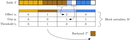
Figure 1: Illustration of the data structure. Input objects are colored by their hash function value. $B=4,\hat{B}=5,m=16,n=15$.

Metadata should use very little space. We therefore limit the maximum offset to a value $\hat{o}$. We also want to support fast search and therefore limit the block size by parameter $\hat{B}$. With these constraints on position and size of blocks, it may not be possible to store all elements of the input set $S$ in table $T$. We therefore allow some elements to be bumped to a backyard $T^{\prime}$. The backyard can be any hash table. Since, hopefully, few elements will be bumped, space and time requirements of the backyard are of secondary concern for now. We adopt the approach from the BuRR retrieval data structure  [10] to base bumping decisions on thresholds: A threshold hash function $\delta(k)$ maps keys to the range $0..\hat{t}-1$. Metadata stores a threshold $t_{i}\in 0..\hat{t}$ for block $b_{i}$ such that elements with $\delta(k)<t_{i}$ are bumped to $T^{\prime}$. We also use the observation from BuRR that overloading the table, i.e., choosing $m<n$ helps to arrive at tables with very few empty cells.

The pseudocode in Figure 2 summarizes a possible representation of the above scheme and gives the resulting search operation. Figure 1 illustrates the data structure. The metadata array $M$ contains an additional slot $M[m/B]$ with a sentinel element helping to ensure that block ends can always be calculated and that no elements outside $T$ are ever accessed. This implementation has tuning parameters $m$, $B$, $\hat{B}$, $\hat{o}$, and $\hat{t}$. We expect that values in $\Theta\!\left(B\right)$ will be good choices for $\hat{B}$, $\hat{o}$, and $\hat{t}$. Concretely, we could for example choose $\hat{B}=2B$ and $\hat{o}=\hat{t}=B$. This leads to space overhead of $\mathcal{O}\!\left(\log B\right)$ bits for the metadata of each block which can be amortized over $B$ elements.

Class SlickHash($m,B,\hat{B},\hat{o},\hat{t}:\mathbb{N}_{+}$, $h:E\rightarrow 0..m/B-1$)

Class MetaData = $\overbrace{o:0..\hat{o}}^{\text{offset}}\times\overbrace{g:0..\hat{B}}^{\text{gap}}\times\overbrace{t:0..\hat{t}}^{\text{threshold}}$

$T$ : Array $[0..m-1]$ of $E$//  main table

$M$${}={}$$(0,B,0)^{m/B}\circ(0,0,0)$ : Array $[0..m/B]$ of MetaData

$T^{\prime}$: HashTable//  backyard

Function blockStart($i$: ${\rm Nature}$) return $Bi+o_{i}$

Function blockEnd($i$: ${\rm Nature}$) return $Bi+B+o_{i+1}-g_{i}-1$

Function blockRange($i$: ${\rm Nature}$) return $\text{{\sf blockStart}}(i)..\text{{\sf blockEnd}}(i)$

// locate an element with key $k$ and return a reference in $e$

Function find($k$: $K$, $e$: $E$) : $\left\{{\bf true},{\bf false}\right\}$

$i\mathbin{:=}h(k)$

if $\delta(k)<t_{i}$ then return $T^{\prime}$.find$(k,e)$//  bumped?

if $\exists j\in\text{{\sf blockRange}}(h(k)):\text{{\sf key}}(T[j])=k$ then $e\mathbin{:=}T[j]$; return true//  found

else return false//  not found

Figure 2: Pseudocode for a simple representation of Slick and the operation find.

3.2 Insertion

	Procedure insert($e$: $E$)//  insert element $e$, noop if already present
$k\mathbin{:=}\text{{\sf key}}(e)$; $i\mathbin{:=}h(k)$//  current block
if $\delta(k)<t_{i}$ then $T^{\prime}$.insert$(e)$; return //  $e$ is already bumped
if $\exists j\in\text{{\sf blockRange}}(h(k)):\text{{\sf key}}(T[j])=k$ then return //  already present
if $\overbrace{|\text{{\sf blockRange}}(i)|=\hat{B}}^{\text{block too large}}$ $\vee$$\overbrace{\neg(g_{i}>0\,||\,\text{{\sf slideGapFromLeft}}(i)\,||\,\text{{\sf slideGapFromRight}}(i))}^{\text{no empty slot usable}}$ then
// bump $e$ or some element from block $b_{i}$
$t^{\prime}\mathbin{:=}1+\min\left\{\delta(x):x\in\left\{k\right\}\cup\left\{\text{{\sf key}}(T[j]):j\in\text{{\sf blockRange}}(i)\right\}\right\}$
$t_{i}\mathbin{:=}t^{\prime}$
$j\mathbin{:=}\text{{\sf blockStart}}(i)$
while $j\leq\text{{\sf blockEnd}}(i)$ do //  Scan existing elements. Bump them as necessary
if $\delta(\text{{\sf key}}(T[j]))<t^{\prime}$ then
$T^{\prime}.\text{{\sf insert}}(T[j])$//  move to backyard
$T[j]\mathbin{:=}T[\text{{\sf blockEnd}}(i)]$; $g_{i}\raisebox{0.51663pt}{\hbox{\tt++}}$//  remove from $T$
else $j\raisebox{0.51663pt}{\hbox{\tt++}}$
if $\delta(k)<t^{\prime}$ then $T^{\prime}.\text{{\sf insert}}(e)$;  return
$g_{i}\raisebox{0.51663pt}{\hbox{\tt-}{\tt-}}$; $T[\text{{\sf blockEnd}}(i)]\mathbin{:=}e$//  insert $e$ into an unused slot
return
// Look for a free slot to the right and move it to block $b_{i}$ if successful
Function slideGapFromRight($i_{0}$: ${\rm Nature}$) : $\left\{{\bf true},{\bf false}\right\}$
$i\mathbin{:=}i_{0}$
while $g_{i}=0$ do //  look for a free slot
if $i\geq m/B\vee o_{i}=\hat{o}$ then return false//  further sliding right is impossible
$i\raisebox{0.51663pt}{\hbox{\tt++}}$
$g_{i}\raisebox{0.51663pt}{\hbox{\tt-}{\tt-}}$
while $i>i_{0}$ do //  shift free slot towards block $b_{i_{0}}$
// Slide $b_{i}$ to the right
$T[\text{{\sf blockEnd}}(i)+1]\mathbin{:=}T[\text{{\sf blockStart}}(i)]$
$o_{i}\raisebox{0.51663pt}{\hbox{\tt++}}$
$i\raisebox{0.51663pt}{\hbox{\tt-}{\tt-}}$
$g_{i}\raisebox{0.51663pt}{\hbox{\tt++}}$
return true

Figure 3: Pseudocode for insertion into Slick Hash Tables. Function slideGapFromLeft works similarly to function slideGapFromRight – it scans left looking for a free slot, failing if it encounters an offset of 0. It slides blocks left by moving their last element to the last free slot of the previous block thus decreasing their offset.

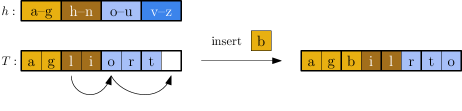
Figure 4: Example for inserting $b$ into a Slick hash table with $B=2$ that previously stored $S=\left\{a,l,g,o,r,i,t,h,m\right\}$.

To insert an element $e$ with key $k$ into a Slick hash table, we first find the block $i=h(k)$ to which $e$ is mapped. Then we check whether the threshold for block $i$ implies that $e$ is bumped. In this case, $e$ must be inserted into the backyard $T^{\prime}$. Otherwise, the data structure invariants give us quite some flexibility how to insert an element. This implies some case distinctions but also allows quite efficient insertions even when the table is already almost full.

A natural goal is to insert $e$ into block $b_{i}$ if this is possible without bumping other elements. The pseudocode in Figure 3 describes one way to do this. This goal is unachievable when $b_{i}$ already contains the maximal number of $\hat{B}$ elements. In that case, we must bump some elements to make room for $e$. Once more there are many ways to achieve this. We describe a fast and simple variant. We look for the smallest increase in the threshold of $b_{i}$ that bumps at least one element from that block (including the new element $e$ itself). We set the threshold accordingly and bump the elements implied by this change. Now, either $e$ is bumped and we are done with the insertion or a free slot after $b_{i}$ is available.

If block $b_{i}$ is not filled to capacity $\hat{B}$, we try to insert $e$ there. However, this may not be directly possible because the gap behind $b_{i}$ could be empty. In that case we can try to slide neighboring blocks to open such a gap. Algorithm 3 does that by first trying to slide $b_{i}$ and some of its left neighbors by one position to the left. This may fail because before finding a nonempty gap, a block with offset 0 may be encountered that cannot be slid to the left. If sliding left failed, function slideGapFromRight tries to slide blocks to the right of $i$ by one position to the right. Once more, this may fail because blocks that already have maximum offset cannot be slid to the right. If there is a range of slidable blocks starting a $b_{i+1}$ and ending at a block followed by a nonempty gap, the actual sliding can be done efficiently by moving only one element per block. Figure 4 gives an example. The first element is appended to the block, filling the first gap element and growing the gap of the previous block.

If neither sliding left nor sliding right can open a gap after block $b_{i}$, the same bumping procedure described for full blocks is used. If sliding was successful (including the case of an empty right-slide for the case that $b_{i}$ already had a nonempty gap), the gap after $b_{i}$ is nonempty and element $e$ can be appended to $b_{i}$.

Corollary 3.1.

A call of insert takes time $\mathcal{O}(\hat{B}+s)+T_{\mathrm{bump}}$ where $s$ is the number of considered blocks and where $T_{\mathrm{bump}}$ is the time incurred in the backyard.

The insertion routine described so far is quite effective in filling the table, however, this gets expensive when the table is almost full. Therefore, in cases where this can happen, one should use a less aggressive insertion routine that bumps if there is no nearby empty slot. What “nearby” means can be controlled with a tuning parameter $\hat{s}$ that controls the maximal number of blocks to slide. Corollary 3.1 implies that $\hat{s}=\mathcal{O}(\hat{B})$ might be a good choice.

We can also consider a more sophisticated insertion routine supported by additional metadata. When routine insert from Figure 3 fails to find a gap to the left or the right, it has identified a blocked cluster (bluster) of full blocks starting with a block with offset $0$ and ending with a block with offset $\hat{o}$. When the table is almost full, blusters can be large and they can persist over many insertions. Thus, it might help to mark blocks inside blusters. An insertion into a bluster can then immediately bump. If blocking flags are represented by a separate bit array, they can be updated in a bit parallel way.

3.3 Bulk Construction

	Procedure greedyBuild($S$: Sequence of $E$)//  build a Slick hash table from $S$
$\text{{\sf bumped}}\mathbin{:=}\left\langle\right\rangle$//  bumped elements
sort $S$ lexicographycally by $(h(e),\delta(e))$
$o\mathbin{:=}0$//  offset
for $i\mathbin{:=}0$ to $m/B-1$ do //  for each block
$b\mathbin{:=}\left\langle e\in S:h(\text{{\sf key}}(e))=i\right\rangle$//  extract block $b_{i}$ from S
$t\mathbin{:=}0$//  threshold for $b_{i}$
excess$\mathbin{:=}$$\max(\overbrace{|b|-\hat{B}}^{|b|\leq\hat{B}},\overbrace{o+iB+|b|-m}^{|T|=m},\overbrace{o+|b|-B-\hat{o}}^{o_{i+1}\leq\hat{o}})$
if $\text{{\sf excess}}>0$ then
for $j\mathbin{:=}1$ to excess do  $\text{{\sf bumped}}.\text{{\sf pushBack}}(b.\text{{\sf popFront}})$//  bump to fit
$t\mathbin{:=}\delta(\text{{\sf bumped}}.\text{{\sf last}})+1$//  adapt threshold
while $|b|>0\wedge\delta(b.\text{{\sf front}})<t$ do
$\text{{\sf bumped}}.\text{{\sf pushBack}}(b.\text{{\sf popFront}})$
$M[i]\mathbin{:=}(o,\max(0,B-o-|b|),t)$//  write metadata for $b_{i}$
for $j\mathbin{:=}0$ to $|b|-1$ do  $T[iB+o+j]\mathbin{:=}b[j]$//  write $b_{i}$ to $T$
$o\mathbin{:=}\max(0,o+|b|-B)$//  next offset
$M[m/B]\mathbin{:=}(0,0,0)$//  sentinel metadata
$T^{\prime}.\text{{\sf build}}(\text{{\sf bumped}})$

Figure 5: Pseudocode for greedy bulk construction of Slick hash tables.

Figure 5 gives pseudocode for a simple greedy algorithm for building a Slick hash table. The elements are sorted by block (and threshold) and then processed block by block. The algorithm tries to fit as many elements into the block as permitted by the constraints that a block must contain at most $\hat{B}$ elements, that the offset must not exceed $\hat{o}$, and that the last available table cell is $T[m-1]$. Violations of these constraint are repaired by bumping a minimal number of elements from the current block.

Theorem 3.2.

Construction of a Slick hash table using greedyBuild can be implemented to run in deterministic time $\mathcal{O}\!\left(|S|\right)$ plus the time for constructing the backyard. As an external memory algorithm, greedy build has the same I/O complexity as sorting.

Proof 3.3.

Using LSD-radix-sort (e.g., see  [30, Section 5.10]), $S$ can be sorted in linear time. All other parts of the algorithm are simple to implement in linear time.

For the external memory variant, we observe that sorting the input can pipeline its sorted output into the construction process, requiring internal memory only for one block at a time.

greedyBuild seems to be a good heuristic for bumping few elements. We are also optimistic that we can prove that using slight overloading, the number of empty cells can be made very small ($me^{-\Omega(\hat{o})}+o(m)$ assuming $\hat{o}=\mathcal{O}\!\left(B\right)$ using an analysis similar to  [10]). Moreover, for fixed values of the tuning parameters, $B$, $\hat{B}$, and $\hat{o}$, we can derive the expected number of empty cells for large $n$ using Markov chains. This allows us to study the impact of different loads $n/m$ analytically.

However, greedyBuild is not optimal. For example, suppose we have $B=\hat{o}=4$, $o_{2}=3$, $|b_{2}|=6$, and all elements in block $b_{2}$ have the same threshold value. Then we have to bump all elements from $b_{2}$ because otherwise $o_{3}=3+6-4=5>4$ violating the constraint on the offset of $b_{3}$. This leaves an empty cell after $b_{2}$. However, it might have been possible to bump one additional element from $b_{1}$ which would have resulted in $o_{2}=2$ so that no elements would have to be bumped from $b_{2}$. We consider to try heuristics that avoid empty cells in a block when they arise, going backwards to bump elements from previous blocks. We can also compute an optimal placement in time $\mathcal{O}\!\left(n\hat{o}\right)$ using dynamic programming.

3.4 Deletion and Backyard Cleaning

	Procedure delete($k$: $K$)//  delete the element with key $k$, noop if not present
if $\delta(k)<t_{i}$ then $T^{\prime}.\text{{\sf delete}}(k)$; return //  element can only be bumped
if $\exists j\in\text{{\sf blockRange}}(h(k)):\text{{\sf key}}(T[j])=k$ then //  found
$T[j]\mathbin{:=}T[\text{{\sf blockEnd}}(h(k))]$//  overwrite deleted element
$g_{h(k)}\raisebox{0.51663pt}{\hbox{\tt++}}$//  extend gap

Figure 6: Pseudocode for deletion from Slick Hash Tables.

Deleting an element is almost as simple as finding it. We just overwrite it with the last element of the block and then increment the gap size. Figure 6 gives pseudocode.

A problem that we have to tackle in applications with many insertions and deletions is that the routines presented so far bump elements but never unbump them. In a situation with basically stable $|S|$, the backyard $T^{\prime}$ will therefore keep growing. This effect can be countered by backyard cleaning. When there are enough empty cells in the primary table $T$ to accommodate $T^{\prime}$, we can reinsert all elements from $T^{\prime}$ into $T$. For each block $b_{i}$, its threshold can be reset to $0$ unless insertion for a backyard element causes bumping. An important observation here is that we never have to bump an element that was in $T$ before backyard cleaning and that we do not have to look at threshold values of those elements. This implies that the $\mathcal{O}(\hat{B})$ term from Corollary 3.1 can be replaced by the number of backyard elements inserted into the affected block. We also expect that we can design a cleaning operation that works more efficiently than inserting backyard elements one-by-one. For example, this can be done by sorting the backyard similar to the build operation and then merging backyard and main table in a single sweep.

Now suppose the backyard has size $\mathcal{O}\!\left(m/B\right)$. Then backyard cleaning can be implemented to run in expected time $\mathcal{O}\!\left(m/B\right)$. If we choose the table size in such a way that $\mathcal{O}\!\left(m\right)$ insert or delete operations cause only $\mathcal{O}\!\left(m/B\right)$ bumps, then the backyard and its management will incur only a factor $\mathcal{O}\!\left(1/B\right)$ overhead in space or time.

4 Variants and Advanced Features

We begin with two variants of Slick that may be of independent interest. Linear cuckoo hashing described in Section 4.1 is almost a special case of Slick that has advantages with respect to the memory hierarchy. Bumped Robin Hood hashing from Section 4.3 is conceptually even simpler than Slick and may allow even faster search at the price of slower insertions.

Section 4.4 is a key result of this section showing how to further reduce space consumption up to the point that the data structure gets succinct. Using bit parallelism allows that while maintaining constant operation times. Section 4.5 briefly discusses how Slick can be parallelized.

4.1 Linear Cuckoo (Luckoo) Hashing

Linear Cuckoo (Luckoo) Hashing is closely related to Slick hashing but more rigidly binds the elements to blocks. Luckoo hashing subdivides the table $T$ into blocks of size $B$ and maintains the invariant that each unbumped element $e\in S$ is either stored in block $h(e)$ or in block $h(e)+1$. This can be implemented as a special case of Slick hashing with $\hat{o}=B$, $\hat{B}=2B$, and the additional constraint that $o_{i}+|b_{i}|\leq 2B$. The main advantage over general Slick hashing is that we can now profit from interleaving metadata with table entries in physical memory blocks of the machine. This way, a find-operation incurs at most two cache faults. Another potential advantage is that storage of offset and gap metadata is now optional as the data structure invariant already defines which $2B$ table cells contain a sought element. This might help with SIMD-parallel implementations.

Luckoo is also useful in the context of truly external memory hash table, e.g., when used for hard disks or SSDs. We obtain a dynamic hash table that is able to almost completely fill the table and where find and delete operations access only 2 consecutive blocks. Insertions look at a consecutive range of blocks. No internal memory metadata is needed. Most external memory hash tables strive to support operations that look at only a single physical block most of the time. We can approximate that by subdividing a physical block into $k$ Slick blocks. That way, find will only access $1+\frac{1}{k}$ physical blocks in expectation.

4.2 Nonbumped Slick – Blocked Robin Hood Hashing (BloRoHo)

Robin Hood hashing  [7] is a variant of linear probing that reduces the cost of unsuccessful searches by keeping elements sorted by their hash function value. Slick without bumping can be seen as a variant of Robin Hood hashing, i.e., elements are sorted by $h(k)$ and metadata tells us exactly where these elements are. We get expected search time $\mathcal{O}\!\left(B\right)$ and expected insertion time bounded by $\mathcal{O}(B+T_{\mathrm{RH}}/B)$ where $T_{\mathrm{RH}}$ is the expected insertion time of Robin Hood hashing. For sufficiently filled tables and not too large $B$, this is faster than basic Robin Hood hashing. Since the bumped version of Slick cannot be asymptotically slower, this also gives us an upper bound on the insertion cost of general Slick.

Actually implementing BloRoHo saves the cost and complications of bumping but pays with giving up worst-case constant find. It also has to take care that metadata appropriately represents all offsets which can get large in the worst case. Rehashing or other special case treatments may be needed.

4.3 Bumbed Robin Hood Hashing (BuRoHo)

We get another variant of Robin Hood hashing if we start with basic Robin Hood hashing without offset or gap metadata but allow bumping. We can then enforce the invariant that any unbumped element $e\in S$ is stored in $T[h(e)..h(e)+B-1]$ for a tuning parameter $B$. As in linear probing, empty cells are indicated by a special element $\bot$. Bumping information could be stored in various ways but the most simple way is to store one bit with every table cell $i$ whether elements $e$ with $h(\text{{\sf key}}(e))=i$ are bumped.

Compared to Slick, BuRoHo more directly controls the range of possible table cells that can contain an element and it obviates the need to store offset and gap metadata. Searches will likely be faster than in Slick. However, insertions are considerably more expensive as we have to move around many elements and evaluate their hash functions. In contrast, Slick can skip entire blocks in constant time using the available metadata.

4.4 Succinct Slick

4.4.1 Quotienting

Cleary  [8] describes a variant of linear probing that infers $\log m$ bits of a key $k$ from $h(k)$. To adapt to displacements of elements, this requires a constant number of metadata bits per element. In Slick we can infer $\log\frac{m}{B}$ key bits even more easily from $h(k)$ since the metadata we store anyway already tells us where elements of a block are stored.

To make this work, the keys are represented in a randomly permuted way, i.e., rather than representing a key $k$ directly, we represent $\pi(k)$. We assume that $\pi$ and its inverse $\pi^{-1}$ can be evaluated in constant time and that $\pi:K\rightarrow 0..|K|-1$ behaves like a random permutation. Using a chain of Feistel permutations  [20, 24, 1], this assumption is at least as realistic as the the assumption that a hash function behaves like a random function. Now it suffices to store $k^{\prime}=\pi(k)\bmod m/B$ in block $\pi(k){\bf\ div\ }(m/B)$. To reconstruct a key $k$ stored as $k^{\prime}$ in block $i$, we compute $k=\pi^{-1}(im/B+k^{\prime})$.

With this optimization, the table entries now are stored succinctly except for

1. $\approx\log B$ bits per element that are lost because we only use bucket indices rather than table indices to infer information on the keys.

2. On top of this come $\mathcal{O}\!\left(\log(B)/B\right)$ bits per element of metadata.

3. Space lost due to empty cells in the table.

4. Space for the backyard.

Items 1. and 2. can be hidden in $o(1)$ allowed for succinct data structures. Items 3. and 4. become lower order terms when $B\in\omega(1)$ . Below, we will see how to do that while still having constant time operations.

4.4.2 Bit Parallelism

With the randomly permuted storage of keys, any subset of $f$ key bits can be used as a fingerprint for the key. If we take $\geq\log\hat{B}$ such fingerprint bits, the expected number of fingerprint collisions will be constant. Moreover, for $f=\mathcal{O}(\log\hat{B})$, and $\hat{B}=\mathcal{O}\!\left(\log(n)/\log\log n\right)$, we can use bit parallelism to process all fingerprints of a block in constant time. To also allow bit parallel access to the right fingerprints, we have to store the fingerprints separately from the remaining bits of the elements.

In algorithm theory, bit parallelism can do many things by just arguing that lookup tables solve the problem. However, this is often impractical since these tables incur a lot of space overhead and cache faults while processing only rather small inputs. However, the operations needed for bit parallel Slick are very simple and even supported by SIMD-units of modern microprocessors.

Specifically, find and delete need to replicate the fingerprint of the sought key $k$ and then do a bit parallel comparison with the fingerprints of block $h(k)$. Operation insert additionally needs bit parallism for bumping. By choosing fingerprints large enough to fully encode the thresholds $\delta(\cdot)$, we can determine the elements with minimal fingerprint in a block using appropriate vector-min and vector-compare operations. The elements with minimal fingerprint then have to be bumped one at a time which is possible in constant expected time as the expected number of minima will be a constant for $f\geq\log\hat{B}$.

We can now extend Corollary 3.1:

Corollary 4.1.

For $\hat{B}=\mathcal{O}\!\left(\log(n)/\log\log n\right)$ and $\log|E|=\mathcal{O}\!\left(\log n\right)$, operations find and delete can be implemented to work in constant expected time. The same holds for operation $insert$ if a variant is chosen that slides a constant number of blocks in expectation.

We believe that we can show that constant time operations can be maintained, for example by choosing $m=n+\Theta\!\left(n/B\right)$ when in expectation $\mathcal{O}\!\left(n/B\right)$ elements will be bumped. In this situation, we can afford to choose a nonsuccinct representation for the backyard. Overall, for $B=\mathcal{O}\!\left(\log(n)/\log\log n\right)$ (and $\hat{B}=2B$, $\hat{o}=\Theta\!\left(B\right)$, $\hat{t}>\log B$) we will get

$$\log\binom{|E|}{n}+\mathcal{O}\!\left(n\left(\overbrace{\log B}^{1.}+\overbrace{\frac{\log B}{B}}^{2.}+\overbrace{\frac{\log n}{B}}^{3.}+\overbrace{\frac{\log n}{B}}^{4.}\right)\right)=\log\binom{|E|}{n}+\mathcal{O}\!\left(n(\log\log n)\right)$$

bits of space consumption. Deletion and backyard cleaning can be done as described in Section 3.4.

Even lower space consumption seems possible if we overload the table (perhaps $m=n-\Theta\!\left(B\right)$) and use a succinct table for the backyard (perhaps using non-overloaded Slick). To maintain constant expected insertion time, we can scan the metadata in a bitparallel way in functions slideGapFromLeft/Right. In addition, we limit the search radius to $\mathcal{O}\!\left(B\right)$ blocks. Only if we are successful, we incur a nonconstant cost of $\mathcal{O}\!\left(B\right)$ for actually sliding blocks. Now consider an insert-only scenario. The first $n-\mathcal{O}\!\left(n/B\right)$ elements can be inserted in constant expected time as in the non-overloaded scenario. The remaining $\mathcal{O}\!\left(n/B\right)$ elements will incur insertion cost $\mathcal{O}\!\left(B\right)$, i.e., $\mathcal{O}\!\left(n\right)$ in total.

4.5 Parallel Processing

Many find operations can concurrently access a Slick hash table. Operations insert and delete require some kind of locking as do many other hash table data structures (but, notably, not linear probing; e.g., see  [30, Section 4.6]). Often locking is implemented by subdividing the table into an array of segments that are controlled by one lock variable.

We can parallelize operation build and bulk insert/delete operations by subdividing the table into segments so that different threads performs operations on separate segments of the table. A simple implementation could enforce independent segments by bumping data that would otherwise be slid across segment boundaries. A more sophisticated implementation could use a postprocessing phase that avoids some of this bumping (perhaps once more in parallel).

5 More Related Work

There is a huge amount of work on hash tables. We do not attempt to give a complete overview but concentrate on approaches that are direct competitors or have overlapping ideas.

Compared to linear probing  [28, 16, 31], Slick promises faster operations when the table is almost full. In particular, unsuccessful search, insertion and deletion should profit. Search and delete also offer worst case deterministic performance guarantees when an appropriate backyard is used in contrast to expected bounds for linear probing An advantage for robust library implementations of hashing is that Slick does not require a special empty element. Advantages of linear probing over Slick are simpler implementation, lockfree concurrent operation, and likely higher speed when ample space is available.

Robin Hood hashing  [7] improves unsuccessful search performance of linear probing at the expense of slower insertion. Slick and our bumped Robin Hood variant described in Section 4.3 go one step further – bumping obviates the need to scan large clusters of elements during search and metadata allows skipping them block-wise during insertion.

Hopscotch hashing  [14] and related approaches  [32] store per-cell metadata to accelerate search of linear probing. We see Slick as an improvement over these techniques as it stores much less metadata with better effect – once more because, thanks to bumping, clusters are not only managed but their negative effect on search performance is removed.

Cuckoo hashing  [26, 12, 9, 21] is a simple and elegant way to achieve very high space efficiency and worst case constant find-operations. Its governing invariant is that an element must be located in one of two (or more) blocks determined by individual hash functions. Slick and linear cuckoo hashing (Luckoo) described in Section 4.1 achieve a similar effect by mostly only accessing a single range of table cells and thus improve locality and allow faster insertion.

Bumping and backyards have been used in many forms previously. Multilevel adaptive hashing  [6] and filter hashing  [12] bump elements along a hierarchy of shrinking layers. These approaches do not maintain explicit bumping information which implies that find has to search all levels. In contrast, filtered retrieval  [23] stores several bits of bumping information per element which is fast and simple but requires more space than the per-block bumping information of Slick. In some sense most similar to Slick is bumped ribbon retrieval (BuRR)  [10] which is not a hash table, but a static retrieval data structure whose construction relies on solving linear equation systems.

Seperator hashing  [19, 13, 18] is an approach to external memory hashing that stores per bucket bumping information similar to the thresholds of Slick. However, by rehashing bumped elements into the main table, overloading cannot be used. Also, Slick’s approach of allowing blocks to slide allows a more flexible use of available storage.

Backyard cuckoo hashing hashes elements to statically allocated blocks (called bins there) and bumps some elements to a backyard when these blocks overflow. There is no bumping metadata. The backyard is a cuckoo hash table whose insertion routine is modified. It tries to terminate cuckoo insertion by moving elements back to the primary table. When plugging in concrete values, the space efficiency of this approach suffers from a large number of empty table entries. For example, to achieve space overhead below 10 %, this approach uses blocks of size at least $333$.

Iceberg hashing also hashes elements to statically allocated blocks. Metadata counts overflowing elements but this implies that find still has to search both main table and backyard for overflowing blocks. Iceberg hashing also needs much larger blocks than Slick since no sliding or other balancing approaches besides bumping are used. For example, a practical variant of iceberg hashing  [27] uses $B=64$ and still has 15 % empty cells. A theoretical variant that achieves succinctness  [3] uses blocks of size $\mathcal{O}\!\left(\log^{2}n\right)$ and uses complex metadata inside blocks to allow constant time search.

There has been intensive further theoretical work on achieving succinctness and constant time operations. We refer to  [3, 5] for a recent overviews. Slick does not achieve all the features mentioned in these results, e.g., with respect to stability or high probability bounds. However, Slick is not only simpler and likely more practical than these approaches, but may also improve some of the crucial bounds. For example, the main result in  [5] is a tradeoff between query time proportional to a parameter $k$ and per element space overhead of $\mathcal{O}(\log^{(k)}n)$ bits where Slick achieves a similar effect by simply choosing an appropriate block size without direct impact on query time. Future (theoretical) work on Slick could perhaps achieve $\mathcal{O}\!\left(1\right)$ bits of overhead per element by exploring the remaining flexibility in arranging elements within a block that can encode $\log B-\mathcal{O}\!\left(1\right)$ bits of information per element using a standard trick of implicit algorithms.

PaCHash  [17] is a static hash table that allows storage of the elements without any gaps using a constant number of metadata bits per block. This even works for objects of variable size. It seems difficult though to make PaCHash dynamic and PaCHash-find is likely to be slower as it needs predecessor search in an Elias-Fano encoded monotone sequence of integers in addition to scanning a block of memory.

A technique resembling the sliding approach in Slick are sparse tables used for representing sorted sequences  [15]. Here a sorted array is made dynamic by allowing for empty cells in the array. Insertion is rearranging the elements to keep the gaps well distributed. Slick can slide faster as it is not bound to keep them sorted and bumping further reduces the high reorganization overhead of sparse tables.

6 Conclusions and Future Work

With Slick (and its variants Luckoo and blocked/bumped Robin Hood), we have described an approach to obtain hash tables that are simple, fast and space efficient. We are in the process of implementing and analyzing Slick. This report already outlines a partial analysis but we need to get a more concrete grip on how the insertion time depends on the number of empty slots.

Several further algorithmic improvements and applications suggest themselves. In particular, we believe that Slick can be adapted to be space efficient also when the final size of the table is not known in advance. We believe that Slick can be used to implement a space efficient approximate membership query filter (AMQ, aka Bloom filter). Concretely, space efficient AMQs can be represented as a set of hash values (this can also be viewed as a compressed single shot Bloom filter)  [29]. The successful dynamic quotient filter AMQ  [25, 4, 22] can be viewed as an implementation of this idea using Cleary’s compact hashing  [8]. Doing this with Slick instead promises a better space-performance tradeoff.

On the practical side, an interesting question is whether Slick could help to achieve better hardware hash tables, as its simple find function could in large parts be mapped to hardware (perhaps with a software handled FAIL for bumped elements). Existing hardware hash tables (e.g.,  [11]) seem to use a more rigid non-slidable block structure.

Acknowledgements.

The authors would like to thank Peter Dillinger for early discussions eventually leading to this paper. This project has received funding from the European Research Council (ERC) under the European Union’s Horizon 2020 research and innovation programme (grant agreement No. 882500). Stefan Walzer is funded by the Deutsche Forschungsgemeinschaft (DFG, German Research Foundation) 465963632.

References

- [1] Yuriy Arbitman, Moni Naor, and Gil Segev. Backyard cuckoo hashing: Constant worst-case operations with a succinct representation. In 51st Symposium on Foundations of Computer Science, pages 787–796. IEEE, 2010.
- [2] Muhammad A Awad, Saman Ashkiani, Serban D Porumbescu, Martin Farach-Colton, and John D Owens. Analyzing and implementing GPU hash tables. In Symposium on Algorithmic Principles of Computer Systems (APOCS), pages 33–50. SIAM, 2023.
- [3] Michael A Bender, Alex Conway, Martín Farach-Colton, William Kuszmaul, and Guido Tagliavini. All-purpose hashing. arXiv preprint arXiv:2109.04548, 2021.
- [4] Michael A Bender, Martin Farach-Colton, Rob Johnson, Russell Kraner, Bradley C Kuszmaul, Dzejla Medjedovic, Pablo Montes, Pradeep Shetty, Richard P Spillane, and Erez Zadok. Don’t thrash: How to cache your hash on flash. Proc. VLDB Endow., 5(11):1627–1637, 2012.
- [5] Michael A. Bender, Martin Farach-Colton, John Kuszmaul, William Kuszmaul, and Mingmou Liu. On the optimal time/space tradeoff for hash tables. In Stefano Leonardi and Anupam Gupta, editors, 54th ACM SIGACT Symposium on Theory of Computing (STOC), pages 1284–1297, 2022. doi:10.1145/3519935.3519969.
- [6] Andrei Z Broder and Anna R Karlin. Multilevel adaptive hashing. In 1st ACM-SIAM Symposium on Discrete Algorithms (SODA), pages 43–53, 1990.
- [7] Pedro Celis, Per-Åke Larson, and J. Ian Munro. Robin hood hashing (preliminary report). In 26th Annual Symposium on Foundations of Computer Science (FOCS), pages 281–288. IEEE Computer Society, 1985. doi:10.1109/SFCS.1985.48.
- [8] J. G. Cleary. Compact hash tables using bidirectional linear probing. IEEE Transactions on Computers, C-33(9):828–834, 1984.
- [9] M. Dietzfelbinger and C. Weidling. Balanced allocation and dictionaries with tightly packed constant size bins. Theoretical Computer Science, 380(1–2):47–68, 2007. URL: http://dx.doi.org/10.1016/j.tcs.2007.02.054.
- [10] Peter C. Dillinger, Lorenz Hübschle-Schneider, Peter Sanders, and Stefan Walzer. Fast succinct retrieval and approximate membership using ribbon. In 20th Symposium on Experimental Algorithms (SEA), 2022. best paper award, full paper at https://arxiv.org/abs/2109.01892.
- [11] Abbas Fairouz, Monther Abusultan, and Sunil P. Khatri. A novel hardware hash unit design for modern microprocessors. In IEEE 34th International Conference on Computer Design (ICCD), pages 412–415, 2016. doi:10.1109/ICCD.2016.7753316.
- [12] D. Fotakis, R. Pagh, P. Sanders, and P. Spirakis. Space efficient hash tables with worst case constant access time. Theory of Comp. Syst., 38(2):229–248, 2005.
- [13] Gaston H. Gonnet and Per-Åke Larson. External hashing with limited internal storage. J. ACM, 35(1):161–184, 1988. doi:10.1145/42267.42274.
- [14] Maurice Herlihy, Nir Shavit, and Moran Tzafrir. Hopscotch hashing. In Distributed Computing, 22nd International Symposium (DISC), volume 5218 of LNCS, pages 350–364. Springer, 2008. doi:10.1007/978-3-540-87779-0\_24.
- [15] A. Itai, A. G. Konheim, and M. Rodeh. A sparse table implementation of priority queues. In S. Even and O. Kariv, editors, Proceedings of the 8th Colloquium on Automata, Languages and Programming, volume 115 of LNCS, pages 417–431. Springer, 1981.
- [16] D. E. Knuth. The Art of Computer Programming – Sorting and Searching, volume 3. Addison Wesley, 2nd edition, 1998.
- [17] Florian Kurpicz, Hans-Peter Lehmann, and Peter Sanders. Pachash: Packed and compressed hash tables. In 2023 Proceedings of the Symposium on Algorithm Engineering and Experiments (ALENEX), pages 162–175. SIAM, 2023.
- [18] Per-Ake Larson. Linear hashing with separators—a dynamic hashing scheme achieving one-access. ACM Transactions on Database Systems (TODS), 13(3):366–388, 1988.
- [19] Per-Åke Larson and Ajay Kajla. File organization: Implementation of a method guaranteeing retrieval in one access. Commun. ACM, 27(7):670–677, 1984. doi:10.1145/358105.358193.
- [20] Michael Luby and Charles Rackoff. How to construct pseudorandom permutations from pseudorandom functions. SIAM Journal on Computing, 17(2):373–386, April 1988.
- [21] Tobias Maier, Peter Sanders, and Stefan Walzer. Dynamic space efficient hashing. Algorithmica, 81(8):3162–3185, 2019.
- [22] Tobias Maier, Peter Sanders, and Robert Williger. Concurrent expandable AMQs on the basis of quotient filters. In 18th Symposium on Experimental Algorithms (SEA). Schloss Dagstuhl-Leibniz-Zentrum für Informatik, 2020.
- [23] Ingo Müller, Peter Sanders, Robert Schulze, and Wei Zhou. Retrieval and perfect hashing using fingerprinting. In 13th Symposium on Experimental Algorithms (SEA), volume 8504 of LNCS, pages 138–149. Springer, 2014. doi:10.1007/978-3-319-07959-2_12.
- [24] M. Naor and O. Reingold. On the construction of pseudorandom permutations: Luby-Rackoff revisited. Journal of Cryptology: the journal of the International Association for Cryptologic Research, 12(1):29–66, 1999. URL: citeseer.nj.nec.com/article/naor97construction.html.
- [25] Anna Pagh, Rasmus Pagh, and S. Srinivasa Rao. An optimal Bloom filter replacement. In SODA, pages 823–829. SIAM, 2005. URL: http://doi.acm.org/10.1145/1070432.1070548.
- [26] R. Pagh and F. Rodler. Cuckoo hashing. Journal of Algorithms, 51(2):122–144, 2004.
- [27] Prashant Pandey, Michael A Bender, Alex Conway, Martín Farach-Colton, William Kuszmaul, Guido Tagliavini, and Rob Johnson. IcebergHT: High performance PMEM hash tables through stability and low associativity. arXiv preprint arXiv:2210.04068, 2022.
- [28] W. W. Peterson. Addressing for random access storage. IBM Journal of Research and Development, 1(2), April 1957.
- [29] Felix Putze, Peter Sanders, and Johannes Singler. Cache-, hash- and space-efficient Bloom filters. ACM Journal of Experimental Algorithmics, 14:4:4.4–4:4.18, January 2010. URL: http://doi.acm.org/10.1145/1498698.1594230, doi:10.1145/1498698.1594230.
- [30] P. Sanders, K. Mehlhorn, M. Dietzfelbinger, and R. Dementiev. Sequential and Parallel Algorithms and Data Structures – The Basic Toolbox. Springer, 2019. doi:10.1007/978-3-540-77978-0.
- [31] Peter Sanders, Kurt Mehlhorn, Martin Dietzfelbinger, and Roman Dementiev. Sequential and Parallel Algorithms and Data Structures – The Basic Toolbox. Springer, 2019. doi:10.1007/978-3-540-77978-0.
- [32] Jan Benedikt Schwarz. Using per-cell data to accelerate open addressing hashing schemes. Bachelor thesis, Karlsruhe Institute of Technology, https://algo2.iti.kit.edu/download/tm_ba_jan_benedikt.pdf, May 2019.
- [33] J. C. Shepherdson and H. E. Sturgis. Computability of recursive functions. Journal of the ACM, 10(2):217–255, 1963.
- [34] Mikkel Thorup. Simple tabulation, fast expanders, double tabulation, and high independence. In 2013 IEEE 54th Annual Symposium on Foundations of Computer Science, pages 90–99. IEEE, 2013.