A Neural Lambda Calculus: Neurosymbolic AI meets the foundations of computing and functional programming
Abstract
Over the last decades, deep neural networks based-models became the dominant paradigm in machine learning. Further, the use of artificial neural networks in symbolic learning has been seen as increasingly relevant recently. To study the capabilities of neural networks in the symbolic AI domain, researchers have explored the ability of deep neural networks to learn mathematical constructions, such as addition and multiplication, logic inference, such as theorem provers, and even the execution of computer programs. The latter is known to be too complex a task for neural networks. Therefore, the results were not always successful, and often required the introduction of biased elements in the learning process, in addition to restricting the scope of possible programs to be executed. In this work, we will analyze the ability of neural networks to learn how to execute programs as a whole. To do so, we propose a different approach. Instead of using an imperative programming language, with complex structures, we use the Lambda Calculus (-Calculus), a simple, but Turing-Complete mathematical formalism, which serves as the basis for modern functional programming languages and is at the heart of computability theory. We will introduce the use of integrated neural learning and lambda calculi formalization. Finally, we explore execution of a program in -Calculus is based on reductions, we will show that it is enough to learn how to perform these reductions so that we can execute any program.
keywords:
Machine Learning, Lambda Calculus, Neurosymbolic AI, Neural Networks, Transformer Model, Sequence-to-Sequence Models, Computational Models1 Introduction
In the field of machine learning, there has been a longstanding debate about the best way to approach the task of learning from data. One approach, which has been referred to as rule-based inference, emphasizes the use of explicit logical rules to reason about the data and make predictions or decisions. The other perspective, known as statistical learning, involves using mathematical models to automatically extract patterns and relationships from the data [1, 2]. Recently, deep neural networks have been employed in applications such as speech recognition, machine translation, and handwriting recognition rather than symbolic reasoning tasks. However, advances in the field have resulted in the introduction of models that are changing the landscape and allowing us to tackle a wider range of problems, including symbolic ones, using neural networks. When neural networks are applied to symbolic problems, the result is a hybrid approach that combines the advantages of both. This combination of the two approaches falls under the realm of neurosymbolic AI [3, 4]. This field combines the statistical nature of machine learning with the logical nature of the reasoning in AI [3], and there have been an increasing interest in the area over the last years [5, 6]. This interested is sparkled by the need to build more robust AI models [7], as initially advocated by Valiant and now a subject of increasing interest in AI research [8, 9, 10].
In this work, we intend to explore the capacity of Machine Learning models, specifically, the Transformer [11], to learn to perform computations, a field that has been traditionally seen as being too complex for neural networks to handle. For this, we use a simple but powerful formalism, the Lambda Calculus (-Calculus), as the underlying framework [12].
Goals
The idea of training a machine learning model to perform computations is relatively new and involves teaching the model to understand the underlying logic and rules involved in mathematical operations. The majority of works in this field tend to restrict the domain of the programs the model can take as input. Therefore, our research question is: “Can a Machine Learning model learn to perform computations?”. Considering that computer programs do not have a fixed size, for the machine learning part, we use a sequence-to-sequence (seq2seq) model, which can take inputs and produce outputs of any length. Specifically, we use a model that has been widely used for several kinds of applications and also tested for symbolic tasks, the Transformer [11].
For the computations, we use the -Calculus, a formalism that, although simple and compact, can perform any computation, according to the Church-Turing thesis [13]. In essence, the -Calculus can be seen as a programming language consisting of terms (-terms) that can be subject to reductions. The -Calculus actually is at the core of many modern programming languages, especially the functional ones [14]. The -terms can be viewed as programs and the reductions can be interpreted as computations performed within the formalism. Applying a single reduction to a term represents an one-step computation in the -Calculus. On the other hand, a full computation involves applying reductions successively on a term that has a normal form until it reaches it, i.e., no more reductions are possible. With these ideas in mind, we propose two hypotheses aimed at answering our research question:
-
•
H1: The Transformer model can learn to perform a one-step computation on Lambda Calculus.
-
•
H2: The Transformer model can learn to perform a full computation on Lambda Calculus.
It is clear that the hypothesis H1 is easier to validate than H2 since a one-step computation is simpler to perform than a full computation. Thus, the purpose of these hypotheses is to gradually enhance our comprehension of the subject matter and enable us to provide an answer to our research question.
Related Work
In [15], seq2seq models are used to learn to evaluate short computer programs using an imperative language with the Python syntax. But their domain of programs is restricted as their programs are short and can use just some arithmetic operations, variable assignment, if-statements, and for loops (not nested). Every program prints an integer as output. Our goal is to rather not limit the domain of programs that our model can learn, focusing solely on the syntactic operations performed to achieve the result.
There are some other studies that also have worked towards developing models that learn algorithms or learn to execute computer code, including [16, 17, 18]. However, the domain of these works is restricted to some arithmetical operations or sequence computations (copying, duplicating, sorting). Additional works concentrate on acquiring an understanding of program representation. For example, [19] builds generative models of natural source code, while [20] applies neural networks to determine if two programs are equivalent.
In [11], the Transformer model was first introduced, bringing several key advancements and improvements compared to the state-of-the-art seq2seq models prevalent at that time. This new model boasted improved parallelism, reduced sequential processing requirements, and the ability to handle longer sequences, among other things. These innovative features have contributed to the widespread adoption of the Transformer model in various Machine Learning applications, including some that involve symbolic mathematics. In a study by [21], the Transformer model was applied to learn how to symbolically integrate functions, yielding very promising results. The authors demonstrated that the model was capable of learning how to perform integrals in a way that was both accurate and efficient, outperforming existing methods in many cases. This study highlights the versatility and potential of the Transformer model, making it a valuable tool for tackling a wide range of machine learning tasks, especially in areas that require symbolic reasoning and mathematical operations.
Also, recent developments in chatbot technologies have been enabled by the Transformer model. One example of a chatbot that has emerged as a result of this development is the ChatGPT 111available at: https://openai.com/blog/chatgpt/, which is based on a state-of-the-art AI model, the GPT-3, from [22]. These chatbots can answer questions about a variety of subjects [23], and can also perform some basic symbolic reasoning. However, their symbolic reasoning capability is still limited, as it gives some incorrect answers to very simple questions.
In the present work, we shift the paradigm from the imperative paradigm that all other works have used to the functional paradigm, which is the case for the -Calculus. With this, we try to abstract the idea of learning to compute computer programs to learning to perform reductions on -terms. With this approach, we will show in the sequel that were able to obtain an accuracy of for learning the one-step -reduction on completely random terms and on terms that represent boolean expressions. Also, for the full computation task, we were able to obtain an accuracy of for terms that represent boolean expressions. If we consider the string similarity metric, where we compare how many characters of the -term the model predicted right, the majority of our results were above . With these results, we think that this change in the paradigm and the use of the Transformer model are two improvements that will be relevant in coming researches.
2 The Lambda Calculus: A Summary
Lambda Calculus (-calculus) is known to be a simple and elegant foundation for computation. It is a formal system based on functions. It is based on function abstraction, which captures the notion of function definition, and function application, which captures the notion of the application of a function to its parameters. It is the base for modern functional programming languages, like Racket, Haskell, and others [14]. It was introduced by Alonzo Church in the 1930s, and has become one of the main computational models [24]. This section is based on the work and use the definition of [12].
2.1 Syntax
In this section, we present the syntax of lambda terms. We start with the formal definition, as follows 222In this definition, parenthesis are used around the abstractions and applications, but we use it just when it is necessary to avoid ambiguity:
Definition 1 (-terms).
Let be a countable set of names. The set of -terms is the smallest set such that
(VAR)
(ABS)
(APP)
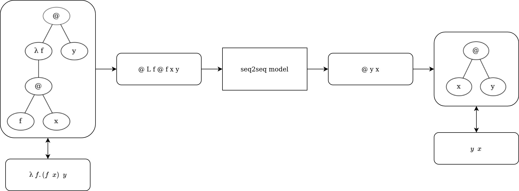
The first rule introduces that every variable is an LT. The second rule says that, given a variable and an LT , the term is an LT, and expresses the notion of function abstraction, being a function that receives one parameter - called - and returns as the result. The third rule says that, given two LT and , is an LT, and expresses the notion of function application, meaning that the function is being called with as its parameter [25]. We can see this syntax as a tree, with the variables as leaves, and the abstraction as a node with one child - the body of the abstraction - and the application as a node with two children - the left and right terms.
2.2 Prefix Notation
Instead of using parenthesis to avoid ambiguities, we can use a prefix notation. Prefix notation (aka Polish Notation) is a very useful way to avoid ambiguities and parenthesis [26]. To achieve this, we traverse the lambda tree with the preorder ordering, where a node is visited, then its left children, and then its right children. This generates terms without parenthesis, but adds the application symbol (@), which is implicit in the infix notation when the application is written as the juxtaposition of two lambda terms. We also change the symbol for this representation using the uppercase letter “L”. For this work, we consider -terms in the prefix notation for the learning tasks. The reason we chose prefix notation is that it offers a well-organized structure, derived from a tree-like representation. This structure allows for a clearer and more straightforward representation of expressions. Furthermore, the prefix notation has a distinct advantage over other notations, as it is unambiguous and eliminates the need for parentheses. This makes it easier to process expressions, particularly for the purposes of learning and understanding complex mathematical concepts.
2.3 Reductions
There are 2 types of reductions in the Lambda Calculus: the alpha-reduction (-reduction) and the beta-reduction (-reduction). These reductions, applied to the -terms, represent the computations in the formalism. The -reduction is responsible for the renaming of variables when necessary. But since we are following the Barendregt convention [12], which states that the name of the variables of interest will always be unique, we don’t need to use the -reduction in this work. The -reduction is, thus, the main reduction of the formalism for us and is based on the substitution operation. The substitution is the operation that takes a -term and substitutes a variable in it with another -term, similar to what is done in mathematics when a function is applied to an argument. The substitution of a variable in the term by a term is denoted by:
We are not going to dive into the specifics of the substitution operation, which can be seen at [25]. But before the definition of the -reduction, the definition of a redex must be given. Informally, a redex is a part of a term where a substitution can occur, i.e., we have an -abstraction followed by any other term. Formally:
Definition 2 (Redex).
A redex (reducible expression) is any subterm in the format
for which the respective contractum is
In addition, if a term does not have any redexes, the term is a normal form. Otherwise, the term is reducible. Now, the -reduction can be defined as:
Definition 3.
-reduction () is the smallest equivalence relation on Lambda terms such that
The -reduction can be seen as just one-step computation. The multi-step reduction is , and is defined as the reflexive and transitive closure of , as follows:
Definition 4.
is the smallest relation on Lambda terms such that
A term can have a normal form, i.e., be reducible with -reductions until it reaches its normal formal, but it can also not have a normal form, i.e., it can enter a loop and never reach a normal form. For example, the term does not have a normal form, because it -reduces to itself. We say that a term has a normal form when exists a term such that and N is a normal form.
As we have seen, a term can have more than one redex, meaning that when we try to apply the -reduction on a term, we can have multiple possibilities. It is useful to have a strategy to select which redex we want to reduce at each step of the computation. Formally,
Definition 5 (Evaluation Strategy).
An evaluation strategy is a function that chooses a single redex for every reducible term.
The two most usual evaluation strategies are: (i) lazy evaluation, where the redex chosen is the leftmost, outermost redex of a term; and (ii) strict evaluation, where the redex chosen is the leftmost, innermost redex of a term.
Choosing the evaluation strategy is very important to clearly define which redex to reduce through the -reduction. Furthermore, it is not just a matter of personal preference, since there is a theorem that says that if a term has a normal form , then the lazy evaluation strategy will always reach from , in a finite number of -reductions. Therefore, in this work, we always use the lazy evaluation strategy when performing -reductions on terms, to assure that, if the term has a normal form, we are able to reach it.
2.4 Encodings and Computations
Lambda terms can be used to represent abstract ideas, such as numbers, lists, boolean formulas, structures, trees, etc. The notion of encoding is well-known in Computer Science, for example, our modern computers operate on binary code, which we use to build abstract ideas from. In Lambda Calculus, the idea is the same. We can use the structure of function abstractions and applications to encode representations for numbers, booleans, strings, etc. The most famous encoding is Church Encoding. Some of these encodings can be found in the work of [25].
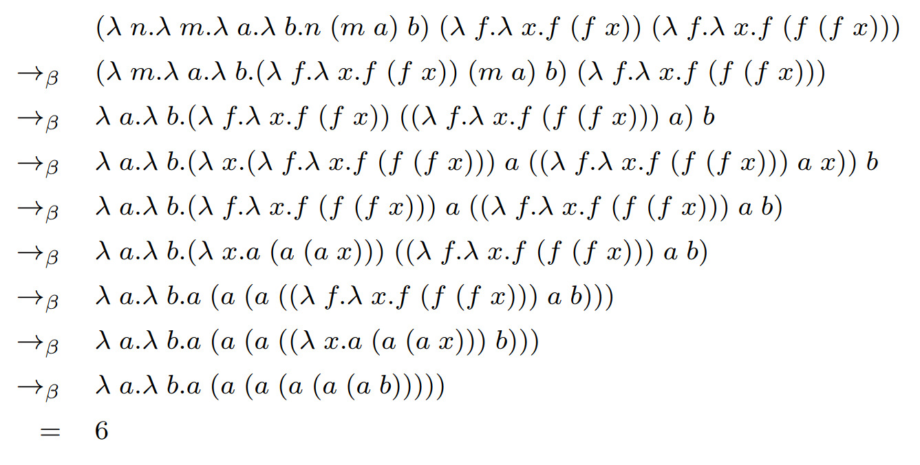
With these encodings, we can execute some computations, such as the multiplication of 2 and 3, as shown in Figure 1.
2.5 De Bruijn Index
The De Bruijn index is a tool to define -terms without having to name the variables [27]. This eliminates the need to worry about variable names when performing a substitution and the need for alpha-equivalence definition. This approach can be beneficial for us, since the terms are agnostic to the variable naming and are simpler, in the sense that they are shorter.
Basically, it just replaces the variable names for natural numbers. The abstraction no longer has a variable name, and every occurrence of a variable is represented by a number, that indicates at which abstraction it is binded. These nameless terms are called de Bruijn terms, and the numeric variables are called de Bruijn indices [28]. For the sake of simplicity, we denote the free variables with the number , and the indices of the bound variables start at . This notation works by assuming that each de Bruijn indice corresponds to the number of binders (abstractions) that the variable is under. This notation can also be used in the prefix manner. We are going to use it to compare with the traditional notation and see if there is any advantage in using a notation with no variable names for the tasks we are interested in.
3 On Machine Learning and Neurosymbolic AI
Machine Learning (ML) is a subfield of AI that involves the development of algorithms and models that can learn from data to make predictions or decisions. ML algorithms can be trained on vast amounts of data, allowing them to identify patterns and relationships in the data and improve their accuracy over time [29].
In supervised learning, algorithms are trained on labeled data, where the output or target variable is known [29]. These algorithms can be used to make predictions about new, unseen data, such as classifying images or predicting stock prices. Unsupervised learning algorithms are trained on unlabeled data where the output or target variable is not known. These algorithms can be used to identify patterns and relationships in the data, such as clustering data into groups or detecting anomalies in data. Reinforcement learning algorithms are designed to learn from interactions with an environment, where the algorithm receives a reward or penalty for each action it takes. These algorithms can be used in various applications, such as game-playing and robotics. This work focuses on supervised learning, particularly on connectionist AI (neural networks).
3.1 Neurosymbolic AI
Neurosymbolic AI is a field of artificial intelligence that combines the strengths of both symbolic AI and connectionist AI. Symbolic AI represents knowledge in a structured, human-readable form and uses reasoning and rule-based systems to perform tasks. Connectionist AI, on the other hand, represents knowledge as patterns in a network of simple processing units to learn from data. The neurosymbolic models aim to merge the two approaches by incorporating symbolic reasoning and/or representation with the learning and generalization capabilities of neural networks [3].
As we can see in [4], there is not only one form of neurosymbolic AI. In the paper, six different forms are presented, with changes of how and where the two different approaches are combined. In the present work, we use the Neuro: Symbolic Neuro approach, where we take a symbolic domain (the -calculus reductions) and apply it to a neural architecture (the Transformer).
3.2 Neural Networks
Artificial Neural Networks were inspired by the structure and function of the human brain and are designed to process large amounts of data to identify patterns and relationships. Their fundamental unit is the Neuron, which essentially ”activates” when a linear combination of its inputs surpasses a certain threshold. A Neural Network is merely a collection of interconnected neurons whose properties are determined by the arrangement of the neurons and their individual characteristics [30].
These neurons are often organized in layers. The input data is fed into the first layer, and the output of each neuron in a given layer is used as the input for the next layer until the final layer produces the output of the network. The connections between the neurons are represented by weights that are updated during the training process to minimize the error between the predicted output and the actual output.
NNs have been applied to a wide range of tasks, including image classification, speech recognition, and natural language processing, among others. One of the main advantages of NNs is their ability to model non-linear relationships between inputs and outputs. This makes NNs a powerful tool for solving complex real-world problems. However, traditional NNs have fixed-size inputs and outputs, which are not suitable for our desired tasks, which have inputs and outputs of variable sizes.
3.3 Sequence-to-sequence Models
Although neural networks are versatile and effective, they are only suitable for problems where inputs and targets can be represented by fixed-dimensional vector encodings. This is a significant constraint, as many crucial problems are better expressed using sequences of unknown lengths, such as speech recognition and machine translation. It is evident that a versatile method that can learn to translate sequences to sequences without being restricted to a specific domain would be valuable. [31].
Sequence-to-sequence (seq2seq) models emerged from this need. They are a type of deep learning model used for tasks that involve mapping an input sequence to an output sequence of variable length. They have been traditionally applied to various natural language processing tasks, such as machine translation, text summarization, and text generation, among others.
Given that we can see the tasks we want to accomplish in this work as machine translation tasks, we have opted to employ the sequence-to-sequence model for our work. Figure 2 shows the general layout for our algorithm.
3.4 The Transformer Model
The Transformer model is a type of neural network architecture that was introduced in [11]. It is designed to handle sequential data, such as natural language, and has quickly become one of the most popular models for tasks such as natural language processing, machine translation, text classification, and question answering. One of the key innovations of the Transformer model is its use of a self-attention mechanism, which allows the model to dynamically weigh the importance of different parts of the input sequence. This allows the Transformer to capture long-range dependencies in the data, which is particularly useful for processing sequences of variable lengths. Another advantage of the Transformer is its parallelization capacity, which allows it to be trained efficiently on large amounts of data. The Transformer model can be trained in parallel on multiple sequences, which is not possible with other traditional sequence-to-sequence models.
The Transformer was the model chosen for this work for several reasons. First, it has parallelization features, which significantly speed up the training time. Also, it presents better performance than all other seq2seq models on a variety of natural language processing. But, besides the better technical features, the main reason we chose the model is for its self-attention mechanism. To perform the -reduction over lambda terms, it is necessary to substitute every occurrence of the variable in question with the term. So, we think that the self-attention can be used to “pay attention” to every occurrence of the variable in question on the -term when performing the task.
4 Building Experiments
For each of the hypotheses outlined in the introduction, we propose a different task for our model to learn. The hypothesis H1 is related to the task of performing the One-Step Beta Reduction (OBR). This hypothesis claims that the model is able to perform a single reduction step in -Calculus, taking a -term and transforming it according to the -reduction rules.
The hypothesis H2 is related to the task of Multi-Step Beta Reduction (MBR). This hypothesis suggests that the model is able to perform multiple reduction steps in lambda calculus, taking a normalizable -term, i.e., a -term that has a normal form, and transforming it into its normal form through multiple beta reduction steps.
The primary focus of our research question is aligned with the second hypothesis. However, we chose to begin with an easier hypothesis as a starting point. The first task is considered easier because it requires the execution of a single computational step, which is less complex than performing a full computation. This approach enables us to gradually build up our understanding and confidence before moving on to the more challenging second hypothesis.
To support these hypotheses, we generate several datasets for each of the tasks and use these datasets to train machine learning models. By training the models on these datasets, we will determine if the models are able to learn and perform the tasks associated with each hypothesis.
4.1 On Training
To learn the tasks mentioned before, we use a neural model. Since the -terms we are using do not have a fixed size, we need our model to accept inputs of varying lengths and generate outputs accordingly. To achieve this, we use a sequence-to-sequence model (seq2seq), which allows for inputs and outputs of different sizes. Specifically, we use the Transformer model, proposed by [11]. This model has been widely used for different applications, including symbolic ones as demonstrated by [21].
For the hyperparameters, preliminary tests showed us that the parameters used by [21] were good enough for our tasks. If needed, they can be adjusted on the training process. So, the initial hyperparameters are the following:
-
•
Number of encoding layers - 6
-
•
Number of decoding layers - 6
-
•
Embedding layer dimension - 1024
-
•
Number of attention heads - 8
-
•
Optimizer - Adam [34]
-
•
Learning rate -
-
•
Loss function - Cross Entropy
4.1.1 Experimental Setting
The experiments were conducted on a server located in our Machine Learning laboratory, situated at the Informatics Institute - UFRGS. The server has the following configurations:
-
•
CPU: Intel(R) Core(TM) i7-8700 CPU @ 3.20GHz
-
•
RAM: 32 GB (2 x 16 Gb) DDR4 @ 2667 MHz
-
•
GPU: Quadro P6000 with 24 Gb
-
•
OS: Ubuntu 18.04.5 LTS
Our initial aim was to have each training session run for a duration of 12 to 24 hours. Preliminary results showed that each training consisting of epochs with an epoch size of would take between 12h to 30h to complete. So, we chose this arrangement. This configuration allows the model to process a total of equations, which is times the size of the dataset.
With this machine, model, and configuration we are using, we can safely have inputs with up to 250 tokens. With more than that, we end up with memory shortage.
4.2 Lambda Sets and Datasets
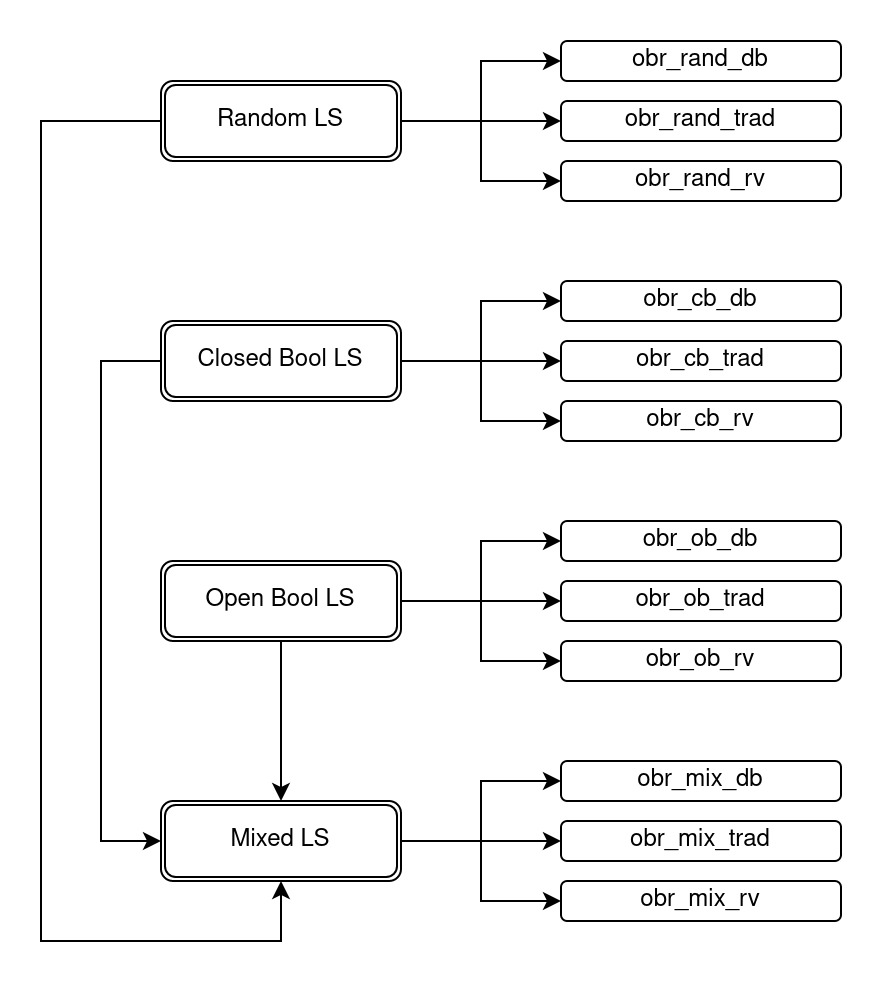
Since, to the best of our knowledge, there are no existing references on generating lambda terms in the literature, we need to develop the generation process from scratch. To generate the datasets that the models are going to train on, we first generate Lambda Sets (LSs) containing only lambda terms. From these LSs, we generate the datasets needed for the trainings. Thus, we generate three LSs:
-
•
Random Lambda Set (RLS): This LS is generated as random and unbiased as possible. Thus, this LS can have terms that do not have a normal form. With the datasets generated from this LS, we want to assert that the model can learn the -reduction, regardless if the input terms represent meaningful computations or if they have a normal form.
-
•
Closed Bool Lambda Set (CBLS): This LS has its terms representing closed boolean expressions. Thus, all terms in this LS have a normal form. With the datasets generated from this LS, we want to assert that the model can learn the -reductions from meaningful computations. Also, these datasets are useful to validate the models trained with the datasets from the RLS, i.e., to validate if the model that learned from random terms can perform meaningful computations.
-
•
Open Bool Lambda Set (OBLS): This LS have its terms representing open boolean expression, with free variables in them. With the datasets generated from this LS, we want to assert that the model can learn the -reductions from meaningful computations, even if the terms have free variables.
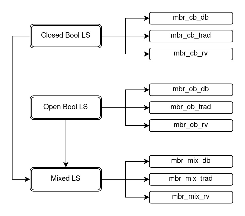
For the One-Step Beta Reduction task, we generate datasets based on the three LSs proposed. However, for the Multi-Step Beta Reduction task, we do not utilize the Random LS to generate datasets, as the terms produced randomly may not have a normal form and result in an infinite loop during the multi-step -reduction. To address this issue, we exclude the RLS and instead use the remaining two LS to generate our datasets.
In addition to the LS mentioned above, for each task, we create an extra LS, which we refer to as a “Mixed Lambda Set” (MLS). These LSs are a combination of the other LSs used on each task. Thus, for the OBR, the MLS is composed of terms coming from the RLS, CBLS, and OBLS in the same proportion. For the MBR, the MLS is formed by terms coming from the CBLS and OBLS, in the same proportion. With these LSs we want to assert that the model can learn from a domain that contemplates several kinds of terms.
Instead of generating only one dataset from each lambda set, we generate three, with different variable naming conventions:
-
•
De Bruijn: This convention uses the prefix de Bruijn notation, presented in Section 2.5. We utilize this convention because it uses a shorter notation and presents a way of representing -terms without the need of naming the variables, which can be beneficial for our model.
-
•
Traditional: This convention uses the prefix traditional notation, presented in Section 2.1 To achieve this version, we take the de Bruijn version and give names to the variables. The order for variable naming used for this convention is the alphabetical order. We utilize this convention because we want to compare the results of the learning process using the de Bruijn notation with the traditional notation.
-
•
Random Vars: This convention also uses the prefix traditional notation. However, for this version, we take the de Bruijn version and give names to the variables using the same algorithm as above, but now using a random order for the variables. We utilize this notation because we want to check if the way we name the variables matter for the accuracies of the models.
Therefore, for the OBR task, we ultimately have a total of 12 datasets, as illustrated in Figure 3. Regarding the MBR task, we have a total of 9 datasets in the end, as depicted in Figure 4. It is noteworthy that the LS utilized for both tasks are identical, meaning that the initial -terms for the datasets that employ the same LS are consistent across both tasks. These datasets provide us with a broad set of test cases to evaluate the performance of our models.
Each dataset contains around one million examples, and we further divide each dataset into training, validation, and test sets. Adhering to the methodology outlined by [21], we allocate a total of about 10 thousand examples for both the validation and test sets. This division of the datasets into training, validation, and test sets allows us to effectively train our models, tune their parameters, and evaluate their performance on independent data. By utilizing a large number of examples in each dataset and following established best practices, we want to ensure that our results are robust and representative of the underlying task.
After generating the datasets, we clean them, deleting pairs that: (i) have undergone -reductions, since we are following the Barendregt Convention; (ii) the first element is already in normal form because we want all pairs to represent -reductions; (iii) appears repeated on the dataset.
4.2.1 Term Sizes
As mentioned in Section 4.1.1, the maximum number of tokens that our configuration allows is 250. So, our generation must respect this limit. For the random dataset, establishing this limit was easy, since there is a parameter in [21] algorithm called max_len that allows us to generate only terms that have a size below this number. However, for the boolean datasets, it was not so simple, since we must take the generated boolean term and convert it to a -term. So, we can not set the max_len for this generation. After conducting several tests, we determined that the parameter for the maximum number of internal nodes to provide to the algorithm should be set to 5. With this configuration, we were able to generate the terms sizes listed in Table 1. While we calculated these sizes using the traditional convention datasets, we expect similar results for the other datasets (with the exception of the de Bruijn convention, which should produce smaller term sizes).
| Task | Dataset | min | max | avg |
|---|---|---|---|---|
| OBR | random | |||
| closed bool | ||||
| open bool | ||||
| mixed | ||||
| MBR | closed bool | |||
| open bool | ||||
| mixed |
4.2.2 Number of Reductions
During this section, it was discussed that for certain Lambda Sets, we iteratively generate the reductions for each term until it reaches its normal form. Thus, another important metric we consider is the number of reductions that each term had to undergo to reach its normal form. This number can be seen as how many computational steps are necessary for evaluating a given term. Table 2 shows the average number of reductions that the terms of each Lambda Set have undergone to generate their respective datasets - for both the OBR and MBR tasks.
| Lambda Set | min | max | avg |
|---|---|---|---|
| closed bool | |||
| open bool | |||
| mixed |
4.3 Code and Implementation
In this work, we utilized two distinct pieces of code. The first piece, adapted from [21], contributed for two main purposes: (i) it assisted in the generation of the lambda sets described above, by generating intermediate -terms and (ii) it handled the learning process. The second piece of code is our own implementation, which deals with the specifics of the -Calculus. Our implementation, coded in Python, is a simulator of the Lambda Calculus, supporting both traditional notation and De Bruijn notation, as well as both notations in prefix and suffix manner. It is entirely based on the substitution operation, which is the fundamental operation of Lambda Calculus.
The lambda calculus simulator is used to generate the -terms for the lambda sets from the intermediate terms generated by the code adapted from [21]. Also, it is used to generate the datasets from the lambda sets, generating the respective reductions from the terms in the LSs. It achieves all this by doing the lambda calculus specifics, such as parsing terms, computing reductions, converting terms between the different notations, etc. This code can be used by anyone that needs a Lambda Calculus parser and/or simulator. It also computes metrics for the datasets and has drawing functions to generate images of the terms as trees, so it can be used for teaching too.
4.4 Experiments and Results
To evaluate the performance of the model during training, the accuracy of the model to predict the data on the test dataset is calculated and recorded after each epoch. This accuracy metric is a measure of how well the model is able to make correct predictions on the data it has seen during training. For each of the models trained, we display a graph showing the evolution of the accuracy of the model (y-axis) over the epochs (x-axis).
The model’s accuracy determines whether the predicted string matches the expected output. However, accuracy may not be the only relevant metric for evaluating the performance of a model in text generation or other similar tasks. In some cases, it may be useful to measure the similarity between the predicted string and the expected one, even if they are not identical. So, additionally, we used a string similarity metric to compare how close the predicted string is to the expected one. For this, we used a common string similarity metric, the Levenshtein distance, which measures the number of changes (insertions, deletions, or substitutions) needed to transform one string into the other [35]. This metric actually provides the absolute difference between the two strings, so we divide this distance by the maximum distance possible between the two strings (which is the length of the longer string) to generate a percentage of dissimilarity. Then, we just subtract this value from 1 to get a percentage of similarity between the two strings. So, for each trained model, we also provide a string similarity value. The formula used is as follows:
As part of our analysis, we also assess the capacity of the models trained with each dataset to evaluate the other datasets. We achieve this by performing additional evaluations with each of the already trained models. For this, we use a model trained with one dataset to evaluate the other datasets that use the same notation and are designed for the same task. For example, we take the model that trained on the obr_rand_trad dataset and evaluate how it performs on the obr_cb_trad, obr_ob_trad and obr_mix_trad datasets.
By evaluating a model on the other datasets, which it did not train on, we can better understand the model’s strengths and weaknesses, as well as its ability to generalize to new data. If the model performs well on other datasets of the same type, it may be a good sign that the model has learned meaningful patterns in the data and can be applied to new, unseen data. If the model performs poorly on other datasets, it may indicate that the model has, for instance, overfit to the original training data or the data was not adequate.
5 Analyzing the Experimental Results
Some trainings experienced oscillation in the accuracy, indicating that the initial learning rate () was too high. So, we had to adjust the learning rate for these trainings. We initially used the same value for all trainings, but decreased it based on the degree of accuracy oscillation. Table 3 shows the final learning rates for each training executed. Although the learning rate was adjusted for different trainings, we kept it consistent for the three conventions in each dataset, for comparison purposes. It is important to note that we did not perform a thorough search for the optimal learning rate, instead selecting a parameter that resulted in a satisfactory and converging accuracy.
| Task | Lambda Set | Learning Rate |
|---|---|---|
| One-Step Beta Reduction | random | |
| closed bool | ||
| open bool | ||
| mixed | ||
| Multi-Step Beta Reduction | closed bool | |
| open bool | ||
| mixed |
5.1 Training Results
This section presents graphs that illustrate the training outcomes for every model trained. The graphs display the model’s accuracy for the test dataset of the respective training dataset as it evolves over the training epochs. Each graph showcases the results for all three conventions utilized in this study: the traditional convention, the random vars convention, and the de Bruijn convention.
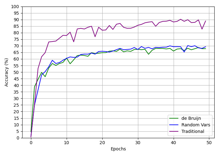
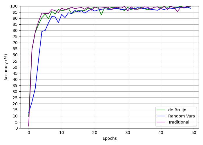
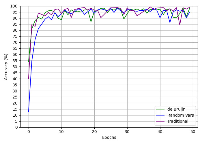
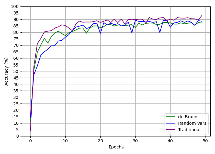
For the OBR task, the training for the random datasets can be seen in Figure 5, the closed bool datasets in Figure 6, the open bool datasets in Figure 7, and the mixed datasets in Figure 8. For the MBR task, the training for the closed bool datasets can be seen in Figure 9, the open bool datasets in Figure 10, and the mix datasets in Figure 11.
Besides the graphs, tables 4 and 5 show the final accuracies, i.e., the accuracy of the last epoch for all the models trained, for both OBR and MBR tasks. The table also depicts the average string similarity percentage, calculated using the Levenshtein distance shown in Section 4.4.
| Lambda Set | Convention | ACC (%) | STR SIM (%) |
|---|---|---|---|
| random | trad | ||
| random vars | |||
| de Bruijn | |||
| closed bool | trad | * | |
| random vars | |||
| de Bruijn | |||
| open bool | trad | ||
| random vars | |||
| de Bruijn | |||
| mixed | trad | ||
| random vars | |||
| de Bruijn |
| Lambda Set | Convention | ACC (%) | STR SIM (%) |
|---|---|---|---|
| closed bool | trad | ||
| random vars | |||
| de Bruijn | |||
| open bool | trad | ||
| random vars | |||
| de Bruijn | |||
| mixed | trad | ||
| random vars | |||
| de Bruijn |
5.2 Evaluation Across Datasets
In this section, we show the results obtained by some additional evaluations with the already trained models, for both the OBR and MBR tasks. We use a model trained with one dataset to evaluate the other datasets that use the same convention and are designed for the same task. For example, we take the model that trained on the obr_cb_db dataset and evaluate how it performs on the obr_rand_db, obr_ob_db and obr_mix_db datasets. We use the test datasets to perform these evaluations.
Tables 6 and 7 shows the values found for the evaluations with the trained models, for the OBR and MBR tasks, respectively.
| Convention | Lambda Set | random | closed bool | open bool | mixed | AVERAGE |
|---|---|---|---|---|---|---|
| traditional | random | 88.89 | 63.69 | 72.66 | 80.47 | 76.43 |
| closed bool | 0.00 | 99.73 | 7.73 | 35.92 | 35.85 | |
| open bool | 0.04 | 80.01 | 98.82 | 63.79 | 60.67 | |
| mixed | 72.26 | 97.42 | 99.62 | 92.88 | 90.55 | |
| random vars | random | 69.30 | 22.17 | 42.27 | 64.65 | 49.60 |
| closed bool | 0.05 | 98.10 | 18.82 | 39.26 | 39.06 | |
| open bool | 0.17 | 77.24 | 94.88 | 61.53 | 58.46 | |
| mixed | 65.77 | 83.90 | 85.92 | 88.52 | 81.03 | |
| de Bruijn | random | 67.84 | 47.15 | 58.35 | 61.14 | 58.62 |
| closed bool | 0.00 | 98.16 | 10.96 | 36.87 | 36.50 | |
| open bool | 0.01 | 77.93 | 97.94 | 58.59 | 58.62 | |
| mixed | 65.70 | 96.39 | 98.71 | 87.93 | 87.18 |
| Convention | Lambda Set | closed bool | open bool | mixed | AVERAGE |
|---|---|---|---|---|---|
| traditional | closed bool | 82.75 | 15.85 | 49.66 | 49.42 |
| open bool | 92.21 | 97.70 | 96.86 | 95.59 | |
| mixed | 96.20 | 93.28 | 97.63 | 95.70 | |
| random vars | closed bool | 76.08 | 24.79 | 50.98 | 50.62 |
| open bool | 75.23 | 80.92 | 84.25 | 80.13 | |
| mixed | 72.72 | 50.68 | 76.58 | 66.66 | |
| de Bruijn | closed bool | 82.20 | 20.20 | 57.83 | 53.41 |
| open bool | 90.02 | 97.02 | 95.37 | 94.14 | |
| mixed | 88.43 | 78.64 | 89.99 | 85.69 |
6 Discussion
In this section, the results obtained from the experiments carried out in the study are discussed in detail. The results are analyzed and interpreted to draw conclusions about the objectives of the study.
6.1 Training
In this section, we are going to discuss the results of the trainings presented in Section LABEL:sec:trainings. With these results, we are able to determine which datasets and conventions performed better and try to conjecture some hypotheses about what happened in the trainings.
6.1.1 One-Step Beta Reduction
In the training of the models for the OBR task, it was found that each model achieved an accuracy of at least . However, when only the best conventions were considered, each model achieved a minimum accuracy of . Additionally, one model achieved a remarkable accuracy. These findings can be seen in Table 4, and they highlight the high level of accuracy and effectiveness of the models, particularly when utilizing the optimal conventions, which supports hypothesis H1.
The metric for string similarity can also be seen in Table 4 and indicates that, despite incorrectly predicting some terms, the model was able to accurately predict a significant portion of those terms, with all similarities being at least . If we take only the best conventions, this number goes up to . Also, some models achieved an outstanding performance of over for this metric. Additionally, for example, the model trained with the random dataset with the de Bruijn convention got a final accuracy of . However, the string similarity metric for the same training was . This illustrates how much the model got the incorrect answers close to the correct ones.
Upon analyzing the performance of the models on different datasets, it is evident that the closed bool and open bool datasets were easier to learn compared to other datasets, as we can see in Figures 5, 6, 7 and 8. The boolean datasets achieved good accuracies in a shorter span of time and presented similar results between themselves. The random dataset was the hardest to learn, as shown in figure 5. We think this is due to the absence of more defined patterns among the terms. The mixed dataset, as expected, fell between the random and the boolean datasets in terms of difficulty to learn. However, its accuracy surprised us, since it was the most diverse dataset, meaning that it learned to perform the OBR task both for random and boolean terms, with high accuracies ( for the optimal convention, as shown in Table 4).
It is worth noting that, although the accuracies for the random and the mixed datasets were comparatively lower than those of the boolean datasets, the graphs illustrating their performance present a growing pattern, as illustrated in Figures 5 and 8. This indicates that further training with more epochs could yield higher accuracies for these datasets.
Analyzing the performance of the models that uses different conventions in Table 4, it can be observed that the traditional convention consistently outperformed the other two conventions, which exhibited similar levels of performance. However, the only training that the convention really made a difference was on the random dataset, which we saw, was the hardest one to learn. We suppose that, for the other datasets, the difference of the convention did not matter because it was so easy for the model to learn that even the “harder” conventions were not a problem. We also think that the traditional convention performed overall better than the other two conventions because for the de Bruijn convention, despite being based on a simpler notation, the beta reduction is more intricate, and consequently, harder to learn. Furthermore, when compared to the random vars convention, the traditional convention, with its ordered naming rule, tends to provide the model with more predictable outcomes.
6.1.2 Multi-Step Beta Reduction
For the training of the models for the MBR task, every model attained a minimum accuracy of . Nevertheless, when considering only the best conventions, each model exhibited an accuracy of at least . Furthermore, one model achieved an exceptional accuracy. These outcomes, which can be seen in Table 5, emphasize the effectiveness and high accuracy of the models, especially when using the optimal conventions, which supports hypothesis H2.
The metric for string similarity, found at Table 5, indicates again that, even though the model made incorrect predictions for some terms, it accurately predicted a significant portion of those terms, with all similarities being no less than . Considering only the best conventions, this number increases to . Additionally, some models performed exceptionally well, achieving up to for this metric. Again, the models that did not obtain a good accuracy got an outstanding performance on this metric. For instance, the model trained with the mixed dataset, using the random vars convention, obtained an accuracy of . Nevertheless, the string similarity metric for the same training was . This shows that for this task, the models also got the wrong predictions very close to the correct ones.
For the closed bool dataset in the MBR task, it is important to notice that the set of possible terms that the model should predict is small (namely, true and false). For the traditional convention and, especially, for the random vars convention, the true and false terms are not always the same term since there are many alpha-equivalent terms for true and false using the English alphabet. But in the DB case, there are only 2 distinct terms for the true and false (“L L 2” and “L L 1”, respectively). Thus, one might expect that the closed bool dataset would be easier to learn since there are only a few possible terms for the model to predict (only two in the DB case), while the open bool, on the other hand, had output terms that differ dramatically from one another.
But the opposite was actually observed, as we can see in Figures 9 and 10. The closed bool dataset was found to be harder to learn than the open bool dataset, with the model that trained on it having significantly lower accuracy than the open bool model, which seems counter-intuitive. Our hypothesis is that, precisely because the terms were so similar in the closed bool dataset, the model resorted to guessing the output term from a limited set of possibilities, based on some features of the inputs, instead of learning to perform the reductions. But, since this was not possible for the open bool dataset, the model was forced to actually learn to perform the multi-step beta reduction on the input terms. The fact that the closed bool model already starts the training with around accuracy also corroborates to our hypothesis that the model is learning to guess from a limited set instead of learning the reductions.
The model trained with the mixed dataset seems to have overcome this issue, as we can see in Figure 11. Considering the traditional convention, the accuracy of the model was similar to the accuracy of the model trained on the open bool dataset, even with half of its terms having come from the closed bool dataset. This actually supports our previous hypothesis, since we think that having more variability on the terms forced the model to learn the reductions instead of only guessing between a small set of possible outcomes.
For the trainings on different conventions, Table 5 shows that the random vars convention had the worst accuracies for the three datasets. However, only the models trained on the open bool and on the mixed datasets presented a large gap between different conventions. We suppose that the naming convention did not change the guessing factor on the learning process for the models that trained on the closed bool. What is interesting is that the de Bruijn convention led to accuracies as good as the traditional convention and significantly better than the random vars convention for the models trained on the open bool and closed bool datasets. This was unexpected since the -reduction on the de Bruijn notation is more intricate than on the traditional notation, which the other two conventions use. For the model trained on the mixed dataset, the order of the different conventions was more aligned with the expected, with the traditional being the best convention, followed by the other two. But this result, although expected, was unusual since the other models did not follow this order.
6.2 Evaluations Across Datasets
In this section, we are going to discuss the results of the evaluations across the datasets presented in Section 5.2. These evaluations can give us some insights as to whether the model really learned the reductions or if it just learned the reductions for that specific set of terms.
6.2.1 One-Step Beta Reduction
The evaluations for this task have yielded promising results, especially for the models trained with the mixed dataset. It produced better average accuracies for all models in the OBR tasks, as seen in Table 6. This shows that, as we expected, these models were able to better capture the diversity of terms present on the different datasets.
The models trained with both boolean datasets performed poorly for the evaluation with the random dataset, with accuracies close to , as we can see in Table 6. We suppose that this happened because the terms in the random dataset are very distinct from the terms from the boolean datasets. Also, since the opposite did not happen, we think that the random dataset contains terms that are actually harder to learn, as we presumed in the previous section.
As expected, almost every model had a better accuracy on the evaluation with the dataset it was trained on rather than with the others, as shown in Table 6. But one result that may be seen as counter-intuitive is the evaluation of the model trained with the mixed dataset. It had better accuracy for the open bool and closed bool datasets for the traditional and de Bruijn conventions. We, again, suppose that this happened because the random dataset is the hardest to learn. Thus, since the mixed dataset has 1/3 of its terms from the random dataset, it ends up being harder than the closed bool and open bool datasets. So, it ends up evaluating better those two datasets than the dataset it was trained with, which contains terms from the random dataset.
Another result that is interesting is that the model trained on the open bool dataset was able to extrapolate and get good accuracies for the evaluation of the closed bool dataset, with a minimum accuracy of . But the opposite did not happen, with accuracies as low as , as we can see in Table 6.
Aside from what was mentioned, the different conventions did not present a significant difference between the evaluations.
6.2.2 Multi-Step Beta Reduction
The evaluations for this task have, again, yielded good results, particularly for the models trained with the open bool dataset. As shown in Table 7, the use of the open bool dataset led to better average accuracies for almost all models in the MBR task.
Table 7 demonstrates that, as anticipated, the majority of models performed better in the evaluations using the dataset they were trained on, as opposed to the other datasets. However, the models trained with the open bool dataset had accuracies quite close to one another for the three datasets evaluated. In fact, it presented a better accuracy for the mixed dataset rather than the dataset it was trained on. We presume that this happened because the model trained with the open bool dataset was able to generalize better than the others.
Again, the models trained with the closed bool did not extrapolate and got good accuracies for the other datasets, especially the closed bool, with accuracies as low as , as seen in Table 7. But the opposite happened, with the open bool models getting a minimum of of accuracy for the closed bool dataset. We think that this happened for the same reason discussed in Section 6.1.2, which is that the model trained on the closed bool dataset just learned to guess the output from a limited set of possible terms, not actually learning the -reduction. Apart from what was stated, the different conventions did not present any main differences between the evaluations.
7 Conclusions and Further Work
In this research, the goal was to explore the following research question: “Can a Machine Learning model learn to perform computations?”. To investigate this, we proposed to use a machine learning model, the Transformer, to learn to perform computations using the -Calculus as the underlying formalism. To accomplish this, the study proposed to teach the model both One-Step Beta Reduction, which represents a one-step computation, and Multi-Step Beta Reduction, which represents a full computation. Thus, two hypotheses were formulated:
-
•
H1: The Transformer model can learn to perform a one-step computation on Lambda Calculus.
-
•
H2: The Transformer model can learn to perform a full computation on Lambda Calculus.
Through comprehensive experimentation and analysis, it was demonstrated that the Transformer model is capable of capturing the syntactic and semantic features of -calculus, allowing for accurate and efficient predictions. The results obtained were positive, with overall good accuracies for both tasks at hand. For the One-Step Beta Reduction, we got accuracies up to %, and string similarity metric of over %. For the Multi-Step Beta Reduction, we obtained accuracies of up to %, and string similarity metric exceeding %. Besides that, the models presented a good generalization performance across different datasets. Due to limitations of hardware and time, our models trained for just 50 epochs. Considering that is a pretty low number compared with substantial trainings of large models, and that we did not do a search for the optimal hyperparameters, we can assure that the accuracy of our models can be even higher than what was presented here.
These results illustrate the effectiveness of the model in learning the desired tasks and support the two hypotheses raised in this study, and, subsequently, the research question proposed. Also, these results showed that the Transformer’s self-attention mechanism is well suited for capturing the dependencies between variables and functions in -Calculus.
We believe that the methods and results presented in this work have yielded some significant outcomes for future researches. The main contributions that have resulted from this research can be summarized as follows:
-
•
Dataset generation: Since datasets for lambda terms and reductions did not exist, we built the generation for these datasets from scratch. These datasets and generation methods can be used in future researches in the lambda calculus domain.
-
•
Lambda calculus learning: The outcomes from learning the reductions of lambda calculus are promising and hold potential implications for future researches in the field of AI and computer programs.
-
•
Functional programming learning: The results obtained in this study can be taken into account for shifting the programming paradigm from imperative to functional in future researches in the field of learning to compute.
Since our work contributes to changing the paradigm traditionally used for the underlying formalism of learned computations, from the imperative to the functional paradigm, we open new possibilities for further research. One key issue is of course, addressing the technological limitations of our work through increased resources. These would provide a way for further advancements. Of course, our contributions are mainly in the proposal of a novel neural lambda calculus, and the experiments we carried out serve to illustrate the potential of our approach in AI and programming languages.
Furthermore, although our research was limited to one formalism - the -calculus, this opens the possibility for further analyzes of other computational calculi. Thus, regarding future research we propose the following:
1. Further training experiments: The current study trained the model for a limited number of epochs. Further research could aim to train the best notation for more epochs to see if performance can be improved.
2. Hyperparameter optimization: The study used a set of predefined hyperparameters for the transformer model. A thorough search for the optimal hyperparameters could be conducted to find the best set of hyperparameters for learning Lambda Calculus.
3. Improved error analysis: The study provided a preliminary error analysis, but further work could aim to conduct a more in-depth error analysis to better understand the types of mistakes the model is making and to identify areas for improvement.
4. Incorporating other formalisms: This study focused on learning Lambda Calculus, but there are other formalisms such as Combinatorial Logic and Turing Machines that could be trained by the model and compared with the current work in future works.
5. Solve typing problems: Learn a typed -Calculus to solve some typing problems, which can be uncomputable: well-typedness, type assignment, type checking, and type inhabitation [28].
6.Learn more complex versions of the -Calculus: Learn the not-pure -Calculus, with numbers and arithmetical and boolean operations already embbeded.
7. Learn to compute a functional programming language: Learn a functional programming language, that is based on -Calculus, such as Haskell or Lisp [36].
8. Learn to detect loops: Use the same methods for the training, but instead of learning to perform the computations, learn to identify if a -term does not have a normal form, i.e., if it is going to enter a loop when applying the reductions.
These future work suggestions have the potential to bring further advancements in the application of machine learning models to the field of symbolic learning. In particular, with respect to programming languages in general, and in particular regarding the use of functional programming as the base paradigm. In summary, we believe that a neurosymbolic approach in which a neural lamda calculus is a foundation can contribute to a deeper understanding of the underlying computational processes in AI.
Supplementary information
The datasets generated during the current study are available at https://bit.ly/lambda_datasets. The repositories for the codes used are available at https://github.com/jmflach/lambda-calculus and https://github.com/jmflach/SymbolicLambda.
Acknowledgments This research is supported in part by CAPES Finance Code 001 and the Brazilian Research Council CNPq.
Declarations
-
•
Funding - This study was funded by CNPq and the CAPES Foundation.
-
•
Conflict of interest/Competing interests - Not applicable.
-
•
Ethics approval - Not applicable.
-
•
Consent to participate - Not applicable.
-
•
Consent for publication - Not applicable.
-
•
Availability of data and materials - The datasets generated during the current study are available at https://bit.ly/lambda_datasets.
-
•
Code availability - The repositories for the codes generated and/or used during the current study are available at https://github.com/jmflach/lambda-calculus and https://github.com/jmflach/SymbolicLambda.
-
•
Authors’ contributions - All authors contributed for this work in the conceptualization of the study, experimentation, writing of the paper, and analyzing the results.
References
- \bibcommenthead
- [1] Rumelhart, D. E. & McClelland, J. L. Parallel Distributed Processing: Explorations in the Microstructure of Cognition, Vol. 1: Foundations (MIT Press, 1986).
- [2] LeCun, Y., Bengio, Y. & Hinton, G. Deep learning. Nature 521, 436 (2015).
- [3] d’Avila Garcez, A. S., Lamb, L. C. & Gabbay, D. Neural-Symbolic Cognitive Reasoning (Springer Berlin Heidelberg, Berlin, Heidelberg, 2009). URL http://link.springer.com/10.1007/978-3-540-73246-4.
- [4] Kautz, H. The Third AI Summer: AAAI Robert Engelmore memorial lecture. AI Magazine 43, 105–125 (2022).
- [5] Garcez, A. d. & Lamb, L. C. Neurosymbolic AI: The 3rd Wave. Artificial Intelligence Review 1–20 (2023).
- [6] Besold, T. R. et al. Neural-symbolic Learning and Reasoning: A survey and interpretation. Neuro-Symbolic Artificial Intelligence: The State of the Art (2022).
- [7] Dietterich, T. G. Steps toward robust artificial intelligence. AI Magazine 38, 3–24 (2017).
- [8] Valiant, L. G. Three problems in computer science. J. ACM 50, 96–99 (2003). URL https://doi.org/10.1145/602382.602410.
- [9] Valiant, L. What needs to be added to machine learning?, TURC ’18, 6 (Association for Computing Machinery, New York, NY, USA, 2018). URL https://doi.org/10.1145/3210713.3210716.
- [10] Marcus, G. & Davis, E. Rebooting AI: Building artificial intelligence we can trust (Vintage, 2019).
- [11] Vaswani, A. et al. Attention is all you need. Advances in neural information processing systems 30 (2017).
- [12] Barendregt, H. The Lambda Calculus: Its Syntax and Semantics North-Holland Linguistic Series (North-Holland, 1984). URL https://books.google.com.br/books?id=eMtTAAAAYAAJ.
- [13] Sipser, M. Introduction to the theory of computation. ACM Sigact News 27, 27–29 (1996).
- [14] Michaelson, G. An Introduction to Functional Programming Through Lambda Calculus Dover books on mathematics (Dover Publications, 2011). URL https://books.google.com.br/books?id=gKvwPtvsSjsC.
- [15] Zaremba, W. & Sutskever, I. Learning to execute. arXiv preprint arXiv:1410.4615 (2014).
- [16] Kaiser, Ł. & Sutskever, I. Neural gpus learn algorithms. arXiv preprint arXiv:1511.08228 (2015).
- [17] Graves, A., Wayne, G. & Danihelka, I. Neural turing machines. arXiv preprint arXiv:1410.5401 (2014).
- [18] Trask, A. et al. Neural arithmetic logic units. Advances in neural information processing systems 31 (2018).
- [19] Maddison, C. & Tarlow, D. Structured generative models of natural source code, 649–657 (PMLR, 2014).
- [20] Mou, L. et al. Building program vector representations for deep learning. arXiv preprint arXiv:1409.3358 (2014).
- [21] Lample, G. & Charton, F. Deep learning for symbolic mathematics. CoRR abs/1912.01412 (2019). URL http://arxiv.org/abs/1912.01412.
- [22] Brown, T. et al. Language models are few-shot learners. Advances in neural information processing systems 33, 1877–1901 (2020).
- [23] Roose, K. The brilliance and weirdness of chatgpt. The New York Times (2022). URL https://www.nytimes.com/2022/12/05/technology/chatgpt-ai-twitter.html.
- [24] Cardone, F. & Hindley, J. R. History of lambda-calculus and combinatory logic. Handbook of the History of Logic 5, 723–817 (2006).
- [25] Machado, R. An introduction to lambda calculus and functional programming (2013).
- [26] Hamblin, C. L. Translation to and from polish notation. The Computer Journal 5 (1962).
- [27] De Bruijn, N. G. Lambda calculus notation with nameless dummies, a tool for automatic formula manipulation, with application to the church-rosser theorem, Vol. 75, 381–392 (Elsevier, 1972).
- [28] Pierce, B. C. Types and programming languages (MIT press, 2002).
- [29] Goodfellow, I., Bengio, Y. & Courville, A. Deep learning Vol. 29 (MIT Press, 2016).
- [30] Russell, S. & Norvig, P. Artificial Intelligence A Modern Approach (2021).
- [31] Sutskever, I., Vinyals, O. & Le, Q. V. Sequence to sequence learning with neural networks. Advances in Neural Information Processing Systems 4, 3104–3112 (2014).
- [32] Lipton, Z. C., Berkowitz, J. & Elkan, C. A critical review of recurrent neural networks for sequence learning. arXiv preprint arXiv:1506.00019 (2015).
- [33] Chung, J., Gulcehre, C., Cho, K. & Bengio, Y. Empirical evaluation of gated recurrent neural networks on sequence modeling. arXiv preprint arXiv:1412.3555 (2014).
- [34] Kingma, D. P. & Ba, J. Adam: A method for stochastic optimization. arXiv preprint arXiv:1412.6980 (2014).
- [35] Levenshtein, V. Binary codes capable of correcting deletions, insertions, and reversals. Soviet physics doklady 10, 707–710 (1966).
- [36] Thompson, S. Haskell: the craft of functional programming (Addison-Wesley, 2011).