Detecting and Characterizing Young Quasars. III.
The Impact of Gravitational Lensing Magnification

Abstract

We test the impact of gravitational lensing on the lifetime estimates of seven high-redshift quasars at redshift $z\gtrsim 6$. The targeted quasars are identified by their small observed proximity zone sizes, which indicate extremely short quasar lifetimes $(t_{Q}\lesssim 10^{5}\text{ yrs})$. However, these estimates of quasar lifetimes rely on the assumption that the observed luminosities of the quasars are intrinsic and not magnified by gravitational lensing, which would bias the lifetime estimates towards younger ages. In order to test possible effects of gravitational lensing, we obtain high-resolution images of the seven quasars with the Hubble Space Telescope (HST) and look for signs of strong lensing. We do not find any evidence of strong lensing, i.e. all quasars are well-described by point sources, and no foreground lensing galaxy is detected. We estimate that the strong lensing probabilities for these quasars are extremely small $(\sim 1.4\times 10^{-5})$, and show that weak lensing changes the estimated quasar lifetimes by only $\lesssim 0.2$ dex. We thus confirm that the short lifetimes of these quasars are intrinsic. The existence of young quasars indicates a high obscured fraction, radiatively inefficient accretion, and/or flickering light curves for high-redshift quasars. We further discuss the impact of lensing magnification on measurements of black hole masses and Eddington ratios of quasars.

1 Introduction

Quasars are the most powerful class of active galactic nuclei (AGNs) and play substantial roles in the evolution of galaxies across cosmic time. Luminous quasars have been discovered up to redshift $z\sim 7.5$ (e.g., Mortlock et al., 2011; Wu et al., 2015; Bañados et al., 2018; Wang et al., 2019; Yang et al., 2020a; Wang et al., 2021), suggesting that supermassive black holes (SMBHs) with masses $M_{\text{BH}}\gtrsim 10^{9}M_{\odot}$ already exist when the universe is less than 1 Gyrs old. These quasars challenge our knowledge about the formation and growth of SMBHs in the early universe. It has been suggested that in order to produce a $10^{9}M_{\odot}$ SMBH at $z=7$, we need either stellar-mass black hole seeds ($M_{\text{BH}}\sim 10^{2}M_{\odot}$, e.g., the remnants of Population III stars) to accrete at super-Eddington rates, or massive black hole seeds with $M_{\text{BH}}\sim 10^{4}M_{\odot}$ that are not trivial to explain (e.g., Inayoshi et al., 2016; Yang et al., 2021). To date, the origin and growth history of these high-redshift quasars are still unclear.

High-redshift quasars are also powerful probes of the intergalactic medium (IGM) and the reionization process. Quasars at $z\sim 6$ have been used to constrain the opacity of the IGM via the Ly$\alpha$ forest (e.g., Fan et al., 2006; Eilers et al., 2018a; Yang et al., 2020b). At $z\gtrsim 7$, the damping wings of quasars enable measurements of the IGM neutral fraction along individual line-of-sights (e.g., Bañados et al., 2018; Yang et al., 2020a; Wang et al., 2020).

Meanwhile, the opaque IGM at $z\gtrsim 6$ offers unique opportunities of investigating the growth history of high-redshift SMBHs. This task is done by measuring the sizes of quasar proximity zones. Specifically, the ultraviolet (UV) photons from a quasar ionize the surrounding IGM, generating a region around the quasar that has enhanced transparency to Ly$\alpha$ photons. This region, known as the proximity zone, can be probed using the rest-frame UV spectrum of the quasar (e.g., Fan et al., 2006; Eilers et al., 2017). The size of the proximity zone $(R_{p})$ increases with the luminosity and the age of the quasar (also referred to as the quasar’s lifetime, $t_{Q}$). It is thus possible to estimate the lifetime of high-redshift quasars by measuring their proximity zone sizes.

In the past few years, we have measured the proximity zone sizes of several tens of quasars and estimated their lifetimes (e.g., Eilers et al., 2017, 2018b, 2020, 2021; Davies et al., 2020b). These quasars show an average quasar lifetime of $t_{Q}\sim 10^{6}$ yrs, consistent with other observations of high-redshift quasars (e.g., Chen & Gnedin, 2018; Bosman et al., 2020; Morey et al., 2021; Khrykin et al., 2021). Interestingly, some quasars in the sample have extraordinarily small proximity zones, indicating short quasar lifetimes of $t_{Q}\lesssim 10^{5}$ yrs. These very young quasars put unique constraints on the models of SMBH growth in the early universe. Eilers et al. (2021) discussed several possible hypotheses to explain the extremely short lifetimes of these quasars, including a long obscured phase of the quasar during which the SMBH can grow without ionizing the surrounding IGM (see also Satyavolu et al., 2022), as well as extremely low radiative efficiency of the mass accretion that would allow the black hole to gain mass in short periods of time.

However, since the size of the quasars’ proximity zones depend on their intrinsic luminosity, the observed short quasar lifetimes could also be explained if strong gravitational lensing magnifies their luminosity, implying that the quasars’ intrinsic luminosity would be much lower. If the young quasars turn out to be strongly lensed, we may have overestimated the production rate of the ionizing photons and thus underestimated the time needed for the quasars to ionize their proximity zones, i.e., the lifetimes of the quasars.

At this point, it is unclear if the young quasars found in our previous studies are gravitationally lensed or not, which makes the interpretation of these quasars complicated. Although ground-based observations have found no signs of strong lensing for these quasars, it is still possible that these quasars are compact lensing systems that are unresolved in ground-based images. One example of this is the quasar J0439+1634, a lensed quasar at $z=6.52$ with a small lensing separation of $\Delta\theta=0\farcs 2$ and a large magnification of $\mu=51$ (Fan et al., 2019). J0439+1634 is unresolved in ground-based imaging even with adaptive optics, and its lensing nature was confirmed only after the Hubble Space Telescope (HST) was able to resolve its lensing structure and detect the foreground deflector galaxy. J0439+1634 is also an excellent example of how lensing magnification affects quasar lifetime estimates. Davies et al. (2020b) shows that the estimated lifetime of J0439+1634 is $t_{Q}\approx 10^{3}$ yrs before accounting for the magnification effect, which becomes $t_{Q}\gtrsim 10^{6}$ yrs after correcting for the lensing magnification.

In this paper, we examine the lensing hypothesis for seven young high-redshift quasars using high-resolution HST images. We look for signs of foreground deflector galaxies and multiple lensed images of the quasars, and estimate the probabilities for these quasars to be strongly lensed. In addition, we develop a method to quantify the impact of lensing magnification on quasar lifetime measurements, where we consider the impact of both weak and strong lensing. This paper is organized as follows. Section 2 describes the sample of young quasars. Section 3 describes the high-resolution HST imaging and data reduction. Section 4 presents the impact of lensing magnification on quasar lifetime measurements. We discuss our results in Section 5 and conclude with Section 6. Throughout this paper, we use a flat $\Lambda$CDM cosmology with $\Omega_{M}=0.3$ and $H_{0}=70\text{ km s}^{-1}\text{Mpc}^{-1}$.

2 The Young Quasar Sample

The sample of young quasars analyzed in this work is gathered from Eilers et al. (2018b), Davies et al. (2020b), and Eilers et al. (2021). We refer the readers to Eilers et al. (2017, 2018b, 2020, 2021) for details about quasar proximity zone size measurements and the quasar lifetime estimations. Here we summarize the basic ideas of these measurements.

Eilers et al. (2017) presents measurements of the proximity zone sizes of 34 quasars using high S/N optical and near-infrared spectra. The proximity zone sizes are measured following the definition in Fan et al. (2006). Specifically, the quasar spectra are normalized by their intrinsic emission, which is estimated using principal component analysis (PCA) trained on low-redshift quasar spectra (e.g., Suzuki, 2006; Pâris et al., 2011; Davies et al., 2018; Bosman et al., 2021). The normalized spectra are then smoothed with a 20Å wide boxcar window to measure the transmission level of the IGM. The edge of the proximity zone is defined by the location where the transmission level drops to 10%. Eilers et al. (2020) further improves the $R_{p}$ measurements of 12 quasars with small proximity zones using updated redshifts based on [C ii] and Mg ii emission lines.

To estimate the age of these quasars, Eilers et al. (2021) run radiative transfer (RT) simulations to model the dependence of $R_{p}$ on quasar lifetimes. Specifically, Eilers et al. (2021) apply the one-dimensional RT simulation code from Davies et al. (2016) on skewers from cosmological hydrodynamical Nyx simulation (Almgren et al., 2013; Lukić et al., 2015). The Nyx simulation was designed for precision cosmological studies of the diffuse gas in the IGM, which includes $4096^{3}$ baryonic (Eulerian) grid elements and dark matter particles. As luminous quasars reside in massive dark matter haloes (e.g., Morselli et al., 2014; Onoue et al., 2018; Meyer et al., 2022; Kashino et al., 2022), Eilers et al. (2021) draw 1,000 skewers in random directions from the centers of the most massive dark matter haloes in the Nyx simulation to model the line-of-sight of observations. The RT code assumes a “lightbulb” model for the quasar (i.e., the quasar turns on and maintains a constant luminosity), and computes the abundance of six particle species in the IGM, i.e., $e^{-}$, H i, H ii, He i, He ii, and He iii. Accordingly, Eilers et al. (2021) compute the transmission of the quasar spectrum and thus the proximity zone size of the quasar along each skewer. The final product of the RT simulation is a distribution of $R_{p}$ given the luminosity and the lifetime of a quasar. By comparing the RT simulations to the observed proximity zone sizes of quasars, Eilers et al. (2021) estimate the lifetime of 10 quasars at $5.7<z<6.5$. Lifetimes of other quasars are estimated in Eilers et al. (2018b), Davies et al. (2020b) and Andika et al. (2020) using the same method.

Figure 1 presents the distribution of $M_{1450}$ (the absolute magnitude at rest-frame 1450Å) and $R_{p}$ of quasars at $z\gtrsim 6$ from the literature. We also plot the $R_{p}$ distribution for quasars at $z\sim 6$ from the RT simulation, which corresponds to a typical lifetime of $t_{Q}=10^{6}$ yrs (e.g., Khrykin et al., 2021). Some quasars show proximity zone sizes smaller than the mean values of RT simulations by more than $1\sigma$, suggesting short lifetimes for these quasars. However, the observed short lifetimes can also be explained by lensing magnification, as discussed in Section 1. The aim of this work is to examine whether these quasars are strongly lensed and investigate the impact of lensing magnification on quasar lifetime measurements.

The young quasar sample of this work consists of seven quasars with short estimated lifetimes ($t_{Q}\lesssim 10^{5}$ yrs), which are marked by red circles in Figure 1. Two of these quasars have archival high-resolution HST images, and we further obtain HST images for the remaining five quasars. The information of these quasars are summarized in Table 1, and the HST observations are described in Section 3 with more details. We note that Andika et al. (2020) analyzed one quasar with a short estimated lifetime of $\log t_{Q}\text{ (yrs)}=3.4$, which exhibits no signs of strong lensing and is not included in our sample.

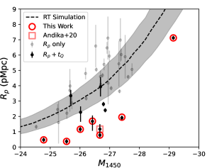
Figure 1: The $M_{1450}-R_{p}$ distribution of $z\sim 6$ quasars from Eilers et al. (2017), Eilers et al. (2020), and Andika et al. (2020). Gray points are quasars with only $R_{p}$ measurements, and black points are quasars with both $R_{p}$ and $t_{Q}$ estimates. The dashed line marks the median proximity zone size predicted by the RT simulation for $z\sim 6$ quasars with $t_{Q}=10^{6}$ yrs, and the gray shaded area shows the $1\sigma$ error. The young quasars analyzed in this work are marked by red circles; these seven quasars have estimated $t_{Q}\lesssim 10^{5}$ yrs, and have high-resolution images taken by HST.

Table 1: The young quasar sample

Quasar	RA	Dec	Redshift	$M_{1450}$	$R_{p}$	$\log t_{Q}$	Reference
	(hh:mm:ss.ss)	(dd:mm:ss.s)		(mag)	(proper Mpc)	(yr)
PSO 004+17	00:17:34.47	+17:05:10.7	5.8165	-26.01	$1.16\pm 0.15$	$3.6^{+0.5}_{-0.4}$	Eilers et al. (2021)
SDSS J0100+2802	01:00:13.02	+28:02:25.8	6.327	-29.14	$7.12\pm 0.13$	$5.1^{+1.3}_{-0.7}$	Davies et al. (2020b)
VDES J0330–4025	03:30:27.92	–40:25:16.2	6.249	-26.42	$1.69^{+0.62}_{-0.35}$	$4.1^{+1.8}_{-0.9}$	Eilers et al. (2021)
PSO J158–14	10:34:46.51	–14:25:15.9	6.0681	-27.41	$1.95\pm 0.14$	$3.8^{+0.4}_{-0.3}$	Eilers et al. (2021)
SDSS J1335+3533	13:35:50.81	+35:33:15.8	5.9012	-26.67	$0.78\pm 0.15$	$3.0\pm 0.4$	Eilers et al. (2018b)
CFHQS J2100-1715	21:00:54.62	–17:15:22.5	6.0806	-25.55	$0.37\pm 0.15$	$2.3\pm 0.7$	Eilers et al. (2021)
CFHQS J2229+1457	22:29:01.65	+14:57:09.0	6.1517	-24.78	$0.47\pm 0.15$	$2.9^{+0.8}_{-0.9}$	Eilers et al. (2021)

Note. — All errors are $1\sigma$ errors.

3 Testing the Strong Lensing Hypotheses with HST Imaging

We use high-resolution HST images to test the strong lensing hypothesis for the young quasars. Each quasar is observed with a red filter and a blue filter. The red filter covers long wavelengths where the quasar has prominent flux. The blue filter covers wavelengths shorter than the rest-frame Lyman limit, where the quasar has no flux due to IGM absorption. In the case of strong lensing, the red image will reveal multiple lensed images of the quasar, and the blue image will detect the foreground lensing galaxy.

Table 2 summarizes the information of the observations. Five of the seven quasars are observed by HST ACS/WFC in the F555W and the F850LP filters (Proposal ID: 16756, PI: Eilers). The other two quasars (SDSS J0100+2802 and VDES J0330-4025) have archival observations by ACS/WFC in the F775W filter and WFC3/IR in the F105W filter, respectively; these two quasars do not have blue images below the quasars’ Lyman limit taken by HST, and we use the $g-$band image from the DESI Legacy Imaging Survey (Dey et al., 2019) as their blue images. J0100+2802 is also observed by ACS/WFC in the F606W filter, which is also presented in this work. The HST images are reduced using the astrodrizzle package (Gonzaga et al., 2012) following the standard procedure.

Figure 2 presents the HST images, where all the quasars appear to be point sources and no foreground lensing galaxy is detected in these fields. In other words, there is no evidence of these quasars being strongly lensed.

To further put quantitative constraints on possible lensing configurations, for each quasar, we fit the red filter image as a point spread function (PSF). We construct PSF models using IRAF task psf based on isolated stars in the field, and use galfit (Peng et al., 2002) to fit the quasar images as a single PSF. Figure 2 shows the residual of the image fitting; all the quasars are well-described by a single PSF with no signs of a second lensed image. We also try to fit the quasar images as two PSFs, which returns the same result as the single-PSF model (i.e., the two PSF components are at the same position).

The HST images thus rule out the hypothesis that the quasars are strongly lensed and have lensing separations larger than the resolution of the HST images. Here we take the PSF full-width half maximum (FWHM; listed in Table 2) as the upper limit of the lensing separation, which is denoted by $\Delta\theta_{\text{max}}$ in the rest of this paper. The non-detection of the foreground lensing galaxy in the blue images also indicate that these quasars are not strongly lensed; however, as we will show in Section 4.1, the upper limits of the lensing separation give stronger constraints on strong lensing probability compared to the blue images.

In principle, it is still possible that these quasars are strongly lensed with small lensing separations that cannot be resolved by HST. Nevertheless, the fraction of strongly-lensed objects at $z\sim 6$ that have lensing separations $\Delta\theta<0\farcs 1$ is only $\sim 1\%$, according to analytical models and mock catalogs of lensing systems (e.g., Yue et al., 2022). As such, it is highly unlikely that the short observed lifetimes of these quasars are results of strong lensing.

Table 2: Imaging of the young quasars

Quasar	Filter	FWHM	Magnitude
		$(^{\prime\prime})$
Red Images (for background quasars)
PSO 004+17	F850LP	$0\farcs 10$	20.78
SDSS J0100+2802	F775W	$0\farcs 10$	21.30
VDES J0330–4025	F850LP	$0\farcs 13$	20.93
PSO J158–14	F850LP	$0\farcs 10$	19.69
SDSS J1335+3533	F105W	$0\farcs 10$	20.03
CFHQS J2100–1715	F850LP	$0\farcs 10$	21.67
CFHQS J2229+1457	F850LP	$0\farcs 10$	22.08
Blue Images (for foreground galaxies)
PSO 004+17	F555W	$0\farcs 1$	$>27.3$
SDSS J0100+2802	Legacy $g$	$1\farcs 6$	$>25.0$
VDES J0330–4025	F555W	$0\farcs 1$	$>27.4$
PSO J158–14	F555W	$0\farcs 1$	$>27.3$
SDSS J1335+3533	Legacy $g$	$2\farcs 1$	$>24.2$
CFHQS J2100–1715	F555W	$0\farcs 1$	$>27.2$
CFHQS J2229+1457	F555W	$0\farcs 1$	$>27.3$

Note. — The F555W, F775W, and the F850LP observations are taken with the HST ACS/WFC. The F105W image is taken with HST WFC3/IR. The PSF FWHMs are estimated using stars in the field. The magnitudes are all AB magnitudes, and the magnitude limits are $5-\sigma$ limits for point sources.

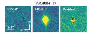
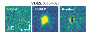
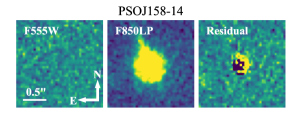
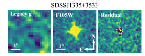
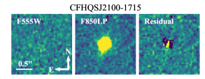
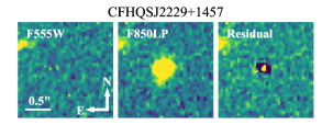
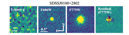
Figure 2: The images of the young quasars. For each quasar, the panels from left to right show the image in a blue filter, the image in a red filter, and the residuals of the red image after subtracting the PSF. All of the quasars are well-described by a single point source, and no foreground lensing galaxies is detected. There is no evidence of strong lensing for these quasars. Note that we include both F606W and F775W images for SDSS J0100+2802, which appears to be a single point source in both images.

3.1 Additional Notes on SDSS J0100+2802

SDSS J0100+2802 was initially reported by Wu et al. (2015) as a ultraluminous quasar with a SMBH mass of $10^{10}M_{\odot}$. SDSS J0100+2802 was later observed by the Atacama Large Millimeter/submillimeter Array with a beam size of $0\farcs 15$ (Fujimoto et al., 2020). The ALMA image of SDSS J0100+2802 exhibits four clumps, which are interpreted as the lensed images of the quasar host galaxy in Fujimoto et al. (2020). The fiducial lensing model suggested by Fujimoto et al. (2020) has an image separation of $\Delta\theta=0\farcs 2$ and a magnification of $\mu=450$.

SDSS J0100+2802 is also a target of the Guaranteed Time Observation program (Proposal ID: 1243, PI: Lilly) of the James Webb Space Telescope (JWST). Eilers et al. (2022) present the NIRCam F115W, F200W, and F356W imaging of SDSS J0100+2802, finding no evidence of strong lensing with separation larger than $0\farcs 05$. The JWST observation is consistent with the HST images reported in this work, and rules out the lensing model suggested by Fujimoto et al. (2020). In the rest of this paper, we use $\Delta\theta_{\text{max}}=0\farcs 05$ as the maximum possible strong lensing separation for SDSS J0100+2802.

3.2 Additional Notes on CFHQS J2229+1457

Figure 2 shows that there is a foreground object in the NE direction that is $1\farcs 03$ away from the quasar J2229+1457. In the HST image, this object can be well described by a Sérsic profile with a half-light radius of $R_{e}=0\farcs 4$, a Sérsic index of $n=3.45$, and an axis ratio of $q=0.57$. The magnitudes of this object is $m_{\text{F555W}}=25.2$ and $m_{\text{F850LP}}=23.8$. Given its detection in the F555W image, this object must be a foreground object, which could introduce a magnification to the background quasar.

Without the spectra and the redshift of the foreground object, we are not able to accurately calculate its contribution to the total magnification of the background quasar. However, we notice that the quasar is not multiply imaged, i.e., the impact of the foreground galaxy can be described by weak lensing. In the Section 4, we will analysis the effect of both strong lensing and weak lensing on quasar lifetime measurements. As such, the potential impact of the foreground object near CFHQS J2229+1457 is covered by the case of weak lensing.

4 The Effect of Lensing Magnification: A Probabilistic Analysis

The observational constraints on lensing models (i.e., the maximum possible lensing separation and the flux limit of the deflector galaxy) are ususally used to derive the probability for the object to be strongly lensed (e.g., Zhe Lee et al., 2022). However, quantifying the implication of the strong lensing probability on quasar lifetime measurements is not straightforward. In this work, we develop a probabilistic method to quantify the impact of lensing magnification on quasar lifetime estimates. We also consider the magnification from weak lensing which is usually ignored in previous studies. Note that the term “strong lensing” means that the object is multiply imaged in this work.

4.1 Strong Lensing Probability

We start our analysis from the a priori probability for an object to be strongly lensed, also known as the strong lensing optical depth $\tau_{m}$. The lensing optical depth describes the probability of a source at a random position to be strongly lensed by a foreground galaxy and is determined by the population of deflector galaxies (e.g., Wyithe & Loeb, 2002; Wyithe et al., 2011; Yue et al., 2022):

$$\tau_{m}=\int_{0}^{z_{s}}dz_{d}\int_{0}^{+\infty}d\sigma\phi(\sigma,z_{d})\frac{d^{2}V_{c}}{d\Omega dz_{d}}\pi\theta_{E}(\sigma,z_{d},z_{s})^{2}$$ (1)

where $z_{s}$ and $z_{d}$ are the redshifts of the source and the deflector, $\frac{d^{2}V_{c}}{d\Omega dz_{d}}$ is the differential comoving volume, $\phi(\sigma,z_{d})$ is the deflector velocity dispersion function (VDF), and $\theta_{E}$ is the Einstein radius of the deflector.

In this work, we use the parameterized VDF suggested by Yue et al. (2022) that matches well with observed VDFs at $z\lesssim 1.5$. We use singular isothermal spheres (SISs) to describe the mass profile of deflectors, which is widely used in modeling the population of lensing systems (e.g., Wyithe et al., 2011; Mason et al., 2015). The Einstein radius of an SIS deflector is given by $\theta_{E}=4\pi\left(\frac{\sigma}{c}\right)^{2}\frac{D_{ds}}{D_{s}}$, where $D_{s}$ and $D_{ds}$ are the angular diameter distances from the observer to the source and from the deflector to the source, and $\sigma$ is the line-of-sight velocity dispersion.

It is useful to notice several properties of SIS lensing systems. An SIS deflector generates two lensed images when the angular separation between the background source and the deflector (denoted by $\beta$) is smaller than the Einstein radius. The two lensed images of the background source are separated by $\Delta\theta=2\theta_{E}$. The lensing magnification is determined by the separation between the source and the deflector in the unit of $\theta_{E}$; in other words, the magnification only depends on the lensing configuration and does not rely on the mass and the redshift of the deflector.

For the quasars in our sample, the HST images rule out lensing models with large image separations. After taking this constraint into consideration, the strong lensing probabilities for these quasars are (see also Zhe Lee et al., 2022, for a similar analysis):

$$\tau_{m}(<\Delta\theta_{\text{max}})=\\ \int_{0}^{z_{s}}dz_{d}\int_{0}^{\sigma_{\text{max}}}d\sigma\phi(\sigma,z_{d})\frac{d^{2}V_{c}}{d\Omega dz_{d}}\pi\theta_{E}(\sigma,z_{d},z_{s})^{2}$$ (2)

where $\sigma_{\text{max}}$ is the maximum velocity dispersion that can generate a compact lensing system allowed by the observation, which is given by $\Delta\theta_{\text{max}}=2\theta_{E}(\sigma_{\text{max}},z_{d},z_{s})$.

Here, $\tau_{m}(<\Delta\theta_{\text{max}})$ gives the probability for a source at a random position to be strongly lensed and has a lensing separation smaller than $\Delta\theta_{\text{max}}$. Using Equation 2, we calculate the value of $\tau_{m}(<\Delta\theta_{\text{max}})$ for each quasar in our sample, which are listed in Table 3. These values are extremely small $(\sim 10^{-5})$, indicating that the observed short lifetimes of the quasars are highly unlikely the results of strong lensing magnification.

In this work, we do not use the flux limit of the deflector galaxy to constrain the strong lensing probability. Specifically, only faint and less massive galaxies are capable of generating small-separation lenses that are unresolved by HST. We estimate the flux of galaxies that have $\sigma<\sigma_{\text{max}}$ using the Faber-Jackson relation from previous observations (Bernardi et al., 2003; Focardi & Malavasi, 2012) and the galaxy spectra templates from Brown et al. (2014). We find that for galaxies at $z\gtrsim 1$ (the typical redshifts for deflector galaxies, e.g., Collett et al., 2013; Mason et al., 2015), the F555W magnitudes are fainter than the image depths in Table 2. In other words, the constraints we obtain from the image separation are more restrictive than the constraints based on the flux limit of a deflector galaxy in our observations. We thus use the non-detection of the deflector galaxies as a cross-check for our results that the young quasars do not exhibit signs of strong lensing.

We also note that the estimated strong lensing probabilities are subject to several systematic errors. Specifically, the galaxy VDFs are not well-determined at $z\gtrsim 1.5$, and Yue et al. (2022) show that the uncertainties of galaxy VDFs introduce a systematic error of $\sim 30\%$ to the estimated lensing optical depth for sources at $z\sim 6$. In addition, we use SIS models for deflectors instead of more realistic elliptical mass distributions. Nevertheless, the strong lensing probabilities are so small that the exact choices of deflector VDFs and lensing models have essentially no impact on our analysis. As we will show in Section 4.2, weak lensing effects dominate the any magnification, and the contribution of strong lensing is negligible.

Table 3: Lensing Probabilities and the inferred quasar lifetimes

Quasar	$\Delta\theta_{\text{max}}$	$\tau_{m}(<\Delta\theta_{\text{max}})$	$\log t_{Q}^{\text{corr}}$
	$(^{\prime\prime})$		(yr)
PSO004+17	$0\farcs 10$	$1.43\times 10^{-5}$	$3.8^{+0.6}_{-0.3}$
J0100+2802	$0\farcs 05$	$4.09\times 10^{-6}$	$4.7^{+2.0}_{-0.6}$
VDESJ0330-4025	$0\farcs 10$	$1.48\times 10^{-5}$	$4.1^{+1.9}_{-0.5}$
PSOJ158-14	$0\farcs 10$	$1.46\times 10^{-5}$	$3.7^{+0.4}_{-0.2}$
SDSSJ1335+3533	$0\farcs 13$	$2.32\times 10^{-5}$	$3.1^{+0.4}_{-0.4}$
CFHQSJ2100-1715	$0\farcs 10$	$1.46\times 10^{-5}$	$2.6^{+0.7}_{-0.8}$
CFHQSJ2229+1457	$0\farcs 10$	$1.47\times 10^{-5}$	$3.2^{+0.8}_{-0.7}$

4.2 Impact of Lensing Magnification on Quasar Lifetime Measurements

We have shown that the strong lensing probability for the young quasars is only $\sim 10^{-5}$. However, the quantitative implication of lensing magnification on the estimated quasar lifetimes is still unclear. In particular, these quasars are subject to the magnification of weak lensing even if they are not strongly lensed. In this Section, we derive the impact of lensing magnification (both strong and weak lensing) on quasar lifetime measurements.

Specifically, we compute $P(\mu)$ by marginalizing the cases of strong lensing and weak lensing, following the method described in Wyithe & Loeb (2002):

$$P(\mu)=\tau_{m}(<\Delta\theta_{\text{max}})P_{s}(\mu)+[1-\tau_{m}(<\Delta\theta_{\text{max}})]P_{w}(\mu)$$ (3)

where $P_{s}(\mu)$ and $P_{w}(\mu)$ are the distribution of magnification generated by strong lensing and weak lensing, respectively. Recall that $\tau_{m}(<\Delta\theta_{\text{max}})$ is the probability of strong lensing.

In this work, we adopt the weak lensing magnification distribution from Mason et al. (2015). Mason et al. (2015) use the code Pangloss (Collett et al., 2013) to compute the weak lensing magnification of random line-of-sights in the Millennium simulation (Springel et al., 2005). We use the SIS lensing model to describe the magnification distribution for strong lensing, i.e., $P_{s}(\mu)=8/\mu^{3}$ (e.g., Yue et al., 2022). This distribution applies to $2<\mu<+\infty$, as the minimum strong-lensing magnification generated by an SIS lens is $\mu_{\text{min}}=2$. Also note that this distribution is independent to the redshifts of the deflector and the background source, as well as the mass of the deflector.

Figure 3 shows the contribution of strong lensing and weak lensing to $P(\mu)$ for a source redshift of $z=6$ and a lensing separation limit of $\Delta\theta_{\text{max}}=0\farcs 1$. The corresponding strong lensing probability is $\tau_{m}(<\Delta\theta_{\text{max}})=1.4\times 10^{-5}$. With such a small probability of strong lensing, the contribution of weak lensing to $P(\mu)$ is about three orders of magnitude higher than that of strong lensing, i.e., we have $P(\mu)\approx P_{w}(\mu)$. Figure 3 demonstrates that the systematic uncertainties of $\tau_{m}(<\Delta\theta_{\text{max}})$ have little impact on the marginalized $P(\mu)$, as we discussed in Section 4.1.

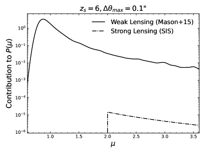
Figure 3: The contribution of weak lensing and strong lensing to the distribution of lensing magnification. This plot shows the case of a source at redshift $z=6$ and a lensing separation limit of $\Delta\theta_{\text{max}}=0\farcs 1$. The dotted dash and the solid lines illustrate the strong lensing term and the weak lensing term in Equation 3. Given the small strong lensing probability $(\sim 1.4\times 10^{-5})$, weak lensing dominates the marginalized distribution of lensing magnification.

We can now write down the marginalized distribution of $t_{Q}$,

$$P(t_{Q})=\iint P(t_{Q}|M^{\text{int}},R_{p})P(M^{\text{int}})P(R_{p})dM^{\text{int}}dR_{p}$$ (4)

where $M^{\text{int}}$ is the intrinsic (i.e., un-magnified) absolute magnitude of the quasar, and $P(M^{\text{int}})$ can be derived from $P(\mu)$ using the relation $M^{\text{int}}=M^{\text{obs}}+2.5\log(\mu)$. We follow the method in Eilers et al. (2022) to obtain $P(t_{Q}|M^{\text{int}},R_{p})$ and $P(R_{p})$. Briefly speaking, $P(t_{Q}|M^{\text{int}},R_{p})$ is calculated using the RT simulations, and $P(R_{p})$ is determined by the redshift uncertainties of the quasars.

Figure 4 illustrates the impact of lensing magnification on quasar lifetime estimates. The left column shows the distribution of $M_{1450}$ and $t_{Q}$ in the RT simulation, given the proximity zone sizes $R_{p}$ of each quasar. The probability distribution of the intrinsic absolute magnitude is marked by the red shaded area, which is determined by the observed absolute magnitude (the red line) and $P(\mu)$. The right column shows the marginalized distribution of $t_{Q}$ for each quasar calculated using Equation 4, with and without taking $P(\mu)$ into consideration. Despite some changes in the shape of the distribution, $P(\mu)$ only shifts the mean values of estimated $t_{Q}$ by $\lesssim 0.2$ dex. Figure 4 thus confirms that the quasars in our sample are intrinsically young with $t_{Q}\lesssim 10^{5}$ yrs, even after taking into account the possible effects of lensing magnification.

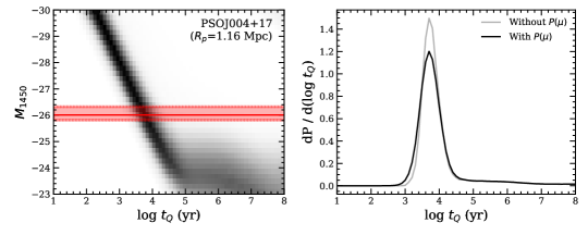
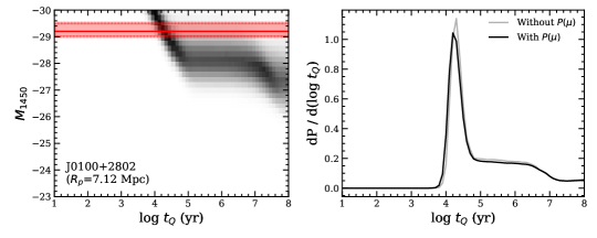
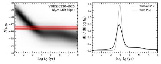
Figure 4: The impact of lensing magnification on quasar lifetime estimation. For each quasar, the left panel presents the distribution of $M_{1450}$ and $t_{Q}$ from the RT simulation, given the quasar’s proximity zone size $R_{p}$. The red solid line marks the observed absolute magnitude of the quasar, and the red shaded area shows the $1\sigma$ (68th percentile) range of the intrinsic absolute magnitude after lensing magnification is considered. The right panel shows the marginalized distribution of quasar lifetimes, $t_{Q}$, with and without considering the effect of lensing magnification. Despite some changes in the shape of $P(t_{Q})$, lensing magnification has little impact on the estimated quasar lifetimes.

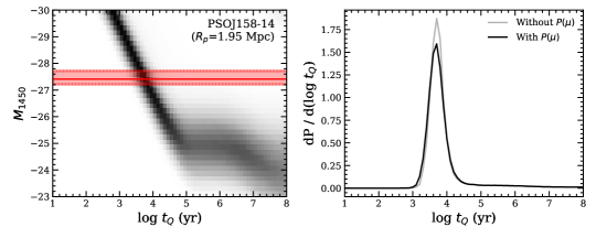
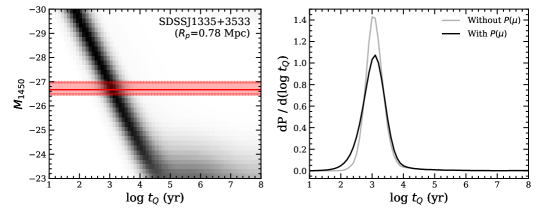
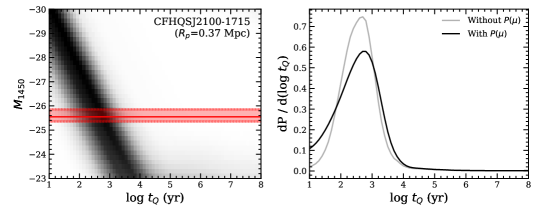
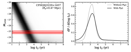
Figure 4 (Continued):

We end this Section by discussing the systematic errors of $t_{Q}$ estimates. Eilers et al. (2021) estimate the systematic errors introduced by the RT simulation to be $\sigma_{\text{sys,}\log t_{Q}}\approx 0.4$, which includes the diversity in quasar spectral energy distributions and reionization models. We suggest that the systematic uncertainty introduced by $P(\mu)$ is much smaller than the systematic uncertainty from the RT simulation. Specifically, the $P_{w}(\mu)$ given by Mason et al. (2015) is very close to other simulations (e.g., Hilbert et al., 2007). Mason et al. (2015) also calculate the $P_{w}(\mu)$ for a range of line-of-sight overdensities, finding that the mean magnification differs by only $\lesssim 0.1$ dex. Accordingly, we estimate the contribution of $P_{w}(\mu)$ to the systematic uncertainty of $t_{Q}$ to be $\lesssim 0.1$ dex. As such, we still take 0.4 dex as the systematic errors of the $t_{Q}$ estimates.

5 Discussion

5.1 The Implication of Young Quasars

Section 4 suggests that the observed short lifetimes ($t_{Q}<10^{5}$ yrs) of the quasars are intrinsic and are not results of lensing magnification. Eilers et al. (2021) report that about $5\%$ of quasars at $z\gtrsim 6$ have lifetimes $t_{Q}<10^{5}$ yrs; our results indicate that the influence of lensing magnification on the observed young quasar fraction is negligible.

Quasars with lifetimes $\lesssim 10^{5}$ yrs put unique constraints on the AGN population and the SMBH growth in the early universe. In the simple model where the black hole is accreting at a constant rate, the SMBH growth can be described by

$$M_{\text{BH}}(t_{Q})=M_{\text{seed}}\times\exp(t_{Q}/t_{S})$$ (5)

where $M_{\text{seed}}$ is the seed black hole mass, and $t_{S}$ is the Salpeter time (Salpeter, 1964, also known as the $e-$folding time) given by

$$t_{S}=45\left(\frac{\epsilon}{1-\epsilon}\right)\left(\frac{L_{\text{bol}}}{L_{\text{Edd}}}\right)^{-1}\text{ Myr}$$ (6)

where $\epsilon$ is the radiation efficiency of the accretion, which is about 0.1 for standard accretion disks (Shakura & Sunyaev, 1973). For seed black holes with $M_{\text{seed}}\sim 10^{2}M_{\odot}$ (e.g., the remnants of Pop III stars), we need $\epsilon\sim 10^{-4}$ to form a SMBH with $M_{\text{BH}}=10^{9}M_{\odot}$ within $10^{5}$ yrs assuming $L_{\text{bol}}\approx L_{\text{Edd}}$. Such a low accretion efficiency is hard to achieve even for hyper-Eddington accretion disks with Eddington ratios $\lambda_{\text{Edd}}>5\times 10^{3}$ (e.g., Inayoshi et al., 2016).

There are two viable explanations for the quasars with extremely short lifetimes. First, the quasars might have experienced an obscured phase where the SMBH is actively accreting material but not ionizing the surrounding IGM. This picture is consistent with hydrodynamical simulations (e.g., Di Matteo et al., 2005; Hopkins et al., 2008), which suggest that merger-triggered AGN evolve from a UV obscured to an unobscured phase. The fraction of accretion time in the UV obscured phase during the entire accretion history of SMBHs can be estimated by the obscured fraction of AGNs. A large obscured fraction of high-redshift AGNs alleviates the difficulty of forming a quasar with a short unobscured, UV luminous lifetime (Davies et al., 2019; Satyavolu et al., 2022). Observations have suggested a high obscured fraction of $\sim 80\%$ (e.g., Vito et al., 2018) for luminous AGNs. Endsley et al. (2022) recently reported a heavily obscured hyperluminous AGN at $z=6.83$ in the 1.5 deg² COSMOS field, suggesting that the obscured fraction of high-redshift luminous quasars might be as high as $\sim 99.5\%$. In the future, a complete sample of AGN is needed to accurately and correctly measure the AGN obscured fraction, which requires multi-wavelength surveys from X-ray to radio (e.g., Lyu et al., 2022).

Second, the quasar lifetime estimates in this work assume a light-bulb lightcurve for the quasars, i.e., the quasar activity only turns on once and never turns off. In contrast, SMBHs may have multiple periods of quasar activity, which offers another explanation for the small proximity zones. Specifically, if the time separation between two periods of quasar activity is sufficiently large, the IGM will become opaque to Ly$\alpha$ photons before the second activity starts due to recombination, even if the first activity episode had ionized the surrounding IGM. In other words, a SMBH can gain mass via previous phases of active accretion, while only the most recent quasar activity is responsible for the formation of the proximity zone of quasars at $z\sim 6$. This effect is analyzed in detail by Davies et al. (2020a) and Satyavolu et al. (2022), who show that the small proximity zone sizes of quasars can be produced by a “flickering” lightcurve (i.e., the quasar regularly turns on and off periodically). This picture agrees with recent phenomenological models of high-redshift SMBH populations (e.g., Li et al., 2022), which suggest that quasars at $z\sim 6$ have experienced multiple periods of active accretion. It is worth noticing that, even with flickering lightcurves, the existence of high-redshift SMBHs at $z\gtrsim 6$ still favors a high obscured AGN fraction of $\gtrsim 70\%$, as argued by Satyavolu et al. (2022).

Based on the above considerations, we argue that the existence of quasars with estimated lifetimes $t_{Q}\lesssim 10^{5}$ yrs is consistent with the picture where these quasars have experienced UV-obscured black hole growth, and might have had several periods of active accretion prior to the current quasar activity, possibly with radiatively inefficient “super-Eddington” accretion disks.

5.2 The Impact of Lensing Magnification on Quasar Property Measurements

In addition to the quasar lifetimes and the trivial case of the quasars’ luminosities, lensing magnification also affects the measurements of other quasar properties. Here we discuss two important examples of such properties, i.e., the SMBH mass and the Eddington ratio of quasars.

The SMBH masses of quasars are often measured using the so-called “single-epoch virial estimators” (e.g., Vestergaard & Peterson, 2006; Vestergaard & Osmer, 2009), which assume that the widths of the broad emission lines originate from the virialized motion of the quasar’s broad line region. Specifically, the black hole mass is calculated using the FWHM of broad emission lines (e.g., H$\alpha$, H$\beta$, Mg ii, C iv) and the continuum luminosity:

$$\log M_{\text{BH}}=a\log\text{FWHM}+b\log\lambda L_{\lambda}+c$$ (7)

with the fiducial parameter values being $a=2$ and $b=0.5$. Note that the FWHM of emission lines is not affected by lensing magnification. Consequently, the apparent (i.e., without correcting for lensing magnification) SMBH mass scales as $M_{\text{BH}}\propto\mu^{0.5}$ (see also Fan et al., 2019).

The Eddington ratio of a quasar is defined as the ratio between its bolometric luminosity and the Eddington luminosity, i.e.,

$$\lambda_{\text{Edd}}=\frac{L_{\text{bol}}}{L_{\text{Edd}}}=\frac{L_{\text{bol}}}{1.26\times 10^{38}\text{ erg s}^{-1}\times(M_{\text{BH}}/M_{\odot})}$$ (8)

Since the apparent SMBH mass $M_{\text{BH}}$ is proportional to $\mu^{0.5}$, according to Equation 8, the apparent Eddington ratio of quasars also scales as $\lambda_{\text{Edd}}\propto\mu^{0.5}$.

Understanding the impact of lensing magnification on these quasar properties is important in the studies of the SMBH population and evolution. In particular, the luminosity functions, the SMBH mass functions and the Eddington ratio distributions play critical roles in the phenomenological models of SMBHs (e.g., Wu et al., 2022; Li et al., 2022). The impact of lensing magnification (especially from weak lensing) should be correctly taken into account in such studies.

Meanwhile, SMBH masses and Eddington ratios provide useful tools in surveys of strongly lensed quasars. In particular, lensed quasars with small lensing separations are usually unresolved in ground-based images and are difficult to distinguish from un-lensed quasars. One possible way to find these lensed quasars is to identify quasars with large apparent SMBH masses and the Eddington ratios and carry out follow-up high-resolution imaging with HST or JWST. This method has been used in the discovery of the currently only known lensed quasar at $z>5$ (Fan et al., 2019) and provided promising lensed quasar candidates (Yue et al. submitted).

6 Conclusion

In this paper, we investigate the strong lensing hypothesis for seven young quasars at $z\gtrsim 6$ with lifetimes of $t_{Q}\lesssim 10^{5}$ yrs, identified via their small proximity zone sizes. We use high-resolution images taken with HST to search for multiple lensed images of the quasars, and use deep images in short wavelengths to detect potential foreground lensing galaxies. We find no evidence of strong lensing for all seven quasars in our sample, essentially ruling out the hypothesis that the observed short quasar lifetimes are results of strong lensing. We further exploit the distribution of weak lensing magnification and derive the impact of lensing magnification on quasar lifetime estimates. Our main results are:

1. The HST images of these seven quasars are well described by point sources, ruling out lensing models with lensing separations larger than the PSF FWHMs. The strong lensing probabilities of these quasars are estimated to be $\sim 1.4\times 10^{-5}$.

2. Given the small strong lensing probabilities, weak lensing dominates the probability distribution of lensing magnification, $P(\mu)$. We compute the probability distribution of $t_{Q}$ for each quasar by marginalizing all possible values of magnifications. Lensing magnification only shifts the mean values of estimated $t_{Q}$ by $\lesssim 0.2$ dex, and we confirm the short lifetimes ($t_{Q}\lesssim 10^{5}$ yrs) of the young quasars.

3. The young quasars with $t_{Q}\lesssim 10^{5}$ yrs are consistent with the picture where high-redshift SMBHs have a high obscured fraction, have had multiple periods of active accretion, and/or have experienced radiatively inefficient super-Eddington accretion phases.

4. We investigate the impact of lensing magnification on measurements of other quasar properties, including the SMBH mass and the Eddington ratio. Such effects should be considered in studies of quasar properties, and provide a viable way to search for compact lensed quasars.

References

- Almgren et al. (2013) Almgren, A. S., Bell, J. B., Lijewski, M. J., Lukić, Z., & Van Andel, E. 2013, ApJ, 765, 39, doi: 10.1088/0004-637X/765/1/39
- Andika et al. (2020) Andika, I. T., Jahnke, K., Onoue, M., et al. 2020, ApJ, 903, 34, doi: 10.3847/1538-4357/abb9a6
- Astropy Collaboration et al. (2013) Astropy Collaboration, Robitaille, T. P., Tollerud, E. J., et al. 2013, A&A, 558, A33, doi: 10.1051/0004-6361/201322068
- Astropy Collaboration et al. (2018) Astropy Collaboration, Price-Whelan, A. M., Sipőcz, B. M., et al. 2018, AJ, 156, 123, doi: 10.3847/1538-3881/aabc4f
- Bañados et al. (2018) Bañados, E., Venemans, B. P., Mazzucchelli, C., et al. 2018, Nature, 553, 473, doi: 10.1038/nature25180
- Bernardi et al. (2003) Bernardi, M., Sheth, R. K., Annis, J., et al. 2003, AJ, 125, 1849, doi: 10.1086/374256
- Bosman et al. (2020) Bosman, S. E. I., Kakiichi, K., Meyer, R. A., et al. 2020, ApJ, 896, 49, doi: 10.3847/1538-4357/ab85cd
- Bosman et al. (2021) Bosman, S. E. I., Ďurovčíková, D., Davies, F. B., & Eilers, A.-C. 2021, MNRAS, 503, 2077, doi: 10.1093/mnras/stab572
- Brown et al. (2014) Brown, M. J. I., Moustakas, J., Smith, J. D. T., et al. 2014, ApJS, 212, 18, doi: 10.1088/0067-0049/212/2/18
- Chen & Gnedin (2018) Chen, H., & Gnedin, N. Y. 2018, ApJ, 868, 126, doi: 10.3847/1538-4357/aae8e8
- Collett et al. (2013) Collett, T. E., Marshall, P. J., Auger, M. W., et al. 2013, MNRAS, 432, 679, doi: 10.1093/mnras/stt504
- Davies et al. (2016) Davies, F. B., Furlanetto, S. R., & McQuinn, M. 2016, MNRAS, 457, 3006, doi: 10.1093/mnras/stw055
- Davies et al. (2019) Davies, F. B., Hennawi, J. F., & Eilers, A.-C. 2019, ApJ, 884, L19, doi: 10.3847/2041-8213/ab42e3
- Davies et al. (2020a) —. 2020a, MNRAS, 493, 1330, doi: 10.1093/mnras/stz3303
- Davies et al. (2020b) Davies, F. B., Wang, F., Eilers, A.-C., & Hennawi, J. F. 2020b, ApJ, 904, L32, doi: 10.3847/2041-8213/abc61f
- Davies et al. (2018) Davies, F. B., Hennawi, J. F., Bañados, E., et al. 2018, ApJ, 864, 143, doi: 10.3847/1538-4357/aad7f8
- Dey et al. (2019) Dey, A., Schlegel, D. J., Lang, D., et al. 2019, AJ, 157, 168, doi: 10.3847/1538-3881/ab089d
- Di Matteo et al. (2005) Di Matteo, T., Springel, V., & Hernquist, L. 2005, Nature, 433, 604, doi: 10.1038/nature03335
- Eilers et al. (2018a) Eilers, A.-C., Davies, F. B., & Hennawi, J. F. 2018a, ApJ, 864, 53, doi: 10.3847/1538-4357/aad4fd
- Eilers et al. (2017) Eilers, A.-C., Davies, F. B., Hennawi, J. F., et al. 2017, ApJ, 840, 24, doi: 10.3847/1538-4357/aa6c60
- Eilers et al. (2018b) Eilers, A.-C., Hennawi, J. F., & Davies, F. B. 2018b, ApJ, 867, 30, doi: 10.3847/1538-4357/aae081
- Eilers et al. (2021) Eilers, A.-C., Hennawi, J. F., Davies, F. B., & Simcoe, R. A. 2021, ApJ, 917, 38, doi: 10.3847/1538-4357/ac0a76
- Eilers et al. (2020) Eilers, A.-C., Hennawi, J. F., Decarli, R., et al. 2020, ApJ, 900, 37, doi: 10.3847/1538-4357/aba52e
- Eilers et al. (2022) Eilers, A.-C., Simcoe, R. A., Yue, M., et al. 2022, arXiv e-prints, arXiv:2211.16261. https://arxiv.org/abs/2211.16261
- Endsley et al. (2022) Endsley, R., Stark, D. P., Lyu, J., et al. 2022, arXiv e-prints, arXiv:2206.00018. https://arxiv.org/abs/2206.00018
- Fan et al. (2006) Fan, X., Strauss, M. A., Becker, R. H., et al. 2006, AJ, 132, 117, doi: 10.1086/504836
- Fan et al. (2019) Fan, X., Wang, F., Yang, J., et al. 2019, ApJ, 870, L11, doi: 10.3847/2041-8213/aaeffe
- Focardi & Malavasi (2012) Focardi, P., & Malavasi, N. 2012, ApJ, 756, 117, doi: 10.1088/0004-637X/756/2/117
- Fujimoto et al. (2020) Fujimoto, S., Oguri, M., Nagao, T., Izumi, T., & Ouchi, M. 2020, ApJ, 891, 64, doi: 10.3847/1538-4357/ab718c
- Gonzaga et al. (2012) Gonzaga, S., Hack, W., Fruchter, A., & Mack, J. 2012, The DrizzlePac Handbook
- Hilbert et al. (2007) Hilbert, S., White, S. D. M., Hartlap, J., & Schneider, P. 2007, MNRAS, 382, 121, doi: 10.1111/j.1365-2966.2007.12391.x
- Hopkins et al. (2008) Hopkins, P. F., Hernquist, L., Cox, T. J., & Kereš, D. 2008, ApJS, 175, 356, doi: 10.1086/524362
- Inayoshi et al. (2016) Inayoshi, K., Haiman, Z., & Ostriker, J. P. 2016, MNRAS, 459, 3738, doi: 10.1093/mnras/stw836
- Kashino et al. (2022) Kashino, D., Lilly, S. J., Matthee, J., et al. 2022, arXiv e-prints, arXiv:2211.08254. https://arxiv.org/abs/2211.08254
- Khrykin et al. (2021) Khrykin, I. S., Hennawi, J. F., Worseck, G., & Davies, F. B. 2021, MNRAS, 505, 649, doi: 10.1093/mnras/stab1288
- Li et al. (2022) Li, W., Inayoshi, K., Onoue, M., & Toyouchi, D. 2022, arXiv e-prints, arXiv:2210.02308. https://arxiv.org/abs/2210.02308
- Lukić et al. (2015) Lukić, Z., Stark, C. W., Nugent, P., et al. 2015, MNRAS, 446, 3697, doi: 10.1093/mnras/stu2377
- Lyu et al. (2022) Lyu, J., Alberts, S., Rieke, G. H., & Rujopakarn, W. 2022, arXiv e-prints, arXiv:2209.06219. https://arxiv.org/abs/2209.06219
- Mason et al. (2015) Mason, C. A., Treu, T., Schmidt, K. B., et al. 2015, ApJ, 805, 79, doi: 10.1088/0004-637X/805/1/79
- Meyer et al. (2022) Meyer, R. A., Decarli, R., Walter, F., et al. 2022, ApJ, 927, 141, doi: 10.3847/1538-4357/ac4f67
- Morey et al. (2021) Morey, K. A., Eilers, A.-C., Davies, F. B., Hennawi, J. F., & Simcoe, R. A. 2021, ApJ, 921, 88, doi: 10.3847/1538-4357/ac1c70
- Morselli et al. (2014) Morselli, L., Mignoli, M., Gilli, R., et al. 2014, A&A, 568, A1, doi: 10.1051/0004-6361/201423853
- Mortlock et al. (2011) Mortlock, D. J., Warren, S. J., Venemans, B. P., et al. 2011, Nature, 474, 616, doi: 10.1038/nature10159
- Onoue et al. (2018) Onoue, M., Kashikawa, N., Uchiyama, H., et al. 2018, PASJ, 70, S31, doi: 10.1093/pasj/psx092
- Pâris et al. (2011) Pâris, I., Petitjean, P., Rollinde, E., et al. 2011, A&A, 530, A50, doi: 10.1051/0004-6361/201016233
- Peng et al. (2002) Peng, C. Y., Ho, L. C., Impey, C. D., & Rix, H.-W. 2002, AJ, 124, 266, doi: 10.1086/340952
- Salpeter (1964) Salpeter, E. E. 1964, ApJ, 140, 796, doi: 10.1086/147973
- Satyavolu et al. (2022) Satyavolu, S., Kulkarni, G., Keating, L. C., & Haehnelt, M. G. 2022, arXiv e-prints, arXiv:2209.08103. https://arxiv.org/abs/2209.08103
- Shakura & Sunyaev (1973) Shakura, N. I., & Sunyaev, R. A. 1973, A&A, 24, 337
- Springel et al. (2005) Springel, V., White, S. D. M., Jenkins, A., et al. 2005, Nature, 435, 629, doi: 10.1038/nature03597
- Suzuki (2006) Suzuki, N. 2006, ApJS, 163, 110, doi: 10.1086/499272
- Vestergaard & Osmer (2009) Vestergaard, M., & Osmer, P. S. 2009, ApJ, 699, 800, doi: 10.1088/0004-637X/699/1/800
- Vestergaard & Peterson (2006) Vestergaard, M., & Peterson, B. M. 2006, ApJ, 641, 689, doi: 10.1086/500572
- Virtanen et al. (2020) Virtanen, P., Gommers, R., Oliphant, T. E., et al. 2020, Nature Methods, 17, 261, doi: 10.1038/s41592-019-0686-2
- Vito et al. (2018) Vito, F., Brandt, W. N., Yang, G., et al. 2018, MNRAS, 473, 2378, doi: 10.1093/mnras/stx2486
- Wang et al. (2019) Wang, F., Yang, J., Fan, X., et al. 2019, ApJ, 884, 30, doi: 10.3847/1538-4357/ab2be5
- Wang et al. (2020) Wang, F., Davies, F. B., Yang, J., et al. 2020, ApJ, 896, 23, doi: 10.3847/1538-4357/ab8c45
- Wang et al. (2021) Wang, F., Yang, J., Fan, X., et al. 2021, ApJ, 907, L1, doi: 10.3847/2041-8213/abd8c6
- Wu et al. (2022) Wu, J., Shen, Y., Jiang, L., et al. 2022, MNRAS, 517, 2659, doi: 10.1093/mnras/stac2833
- Wu et al. (2015) Wu, X.-B., Wang, F., Fan, X., et al. 2015, Nature, 518, 512, doi: 10.1038/nature14241
- Wyithe & Loeb (2002) Wyithe, J. S. B., & Loeb, A. 2002, ApJ, 577, 57, doi: 10.1086/342181
- Wyithe et al. (2011) Wyithe, J. S. B., Yan, H., Windhorst, R. A., & Mao, S. 2011, Nature, 469, 181, doi: 10.1038/nature09619
- Yang et al. (2020a) Yang, J., Wang, F., Fan, X., et al. 2020a, ApJ, 897, L14, doi: 10.3847/2041-8213/ab9c26
- Yang et al. (2020b) —. 2020b, ApJ, 904, 26, doi: 10.3847/1538-4357/abbc1b
- Yang et al. (2021) —. 2021, ApJ, 923, 262, doi: 10.3847/1538-4357/ac2b32
- Yue et al. (2022) Yue, M., Fan, X., Yang, J., & Wang, F. 2022, ApJ, 925, 169, doi: 10.3847/1538-4357/ac409b
- Zhe Lee et al. (2022) Zhe Lee, R., Pacucci, F., Natarajan, P., & Loeb, A. 2022, arXiv e-prints, arXiv:2209.06830. https://arxiv.org/abs/2209.06830