The ALMA REBELS Survey: Discovery of a massive, highly star-forming and morphologically complex ULIRG at $z=7.31{}$

Abstract

We present Atacama Large Millimeter/Submillimeter Array (ALMA) [Cii] and $\sim 158$ $\rm\mu m$ continuum observations of REBELS-25, a massive, morphologically complex ultra-luminous infrared galaxy (ULIRG; $L_{\rm IR}=$ $1.5^{+0.8}_{-0.5}\times 10^{12}$ L_⊙) at $z=7.31$, spectroscopically confirmed by the Reionization Era Bright Emission Line Survey (REBELS) ALMA Large Programme. REBELS-25 has a significant stellar mass of $M_{*}=\mbox{$8^{+4}_{-2}\times 10^{9}$}{}~{}\mbox{M${}_{\odot}$}{}$. From dust-continuum and ultraviolet observations, we determine a total obscured + unobscured star formation rate of SFR $=\mbox{$199^{+101}_{-63}$}{}~{}\mbox{M${}_{\odot}$}~{}\mbox{${\rm yr}$}^{-1}$. This is about four times the SFR estimated from an extrapolated main-sequence. We also infer a [Cii]-based molecular gas mass of $M_{{\rm H}_{2}}=\mbox{$5.1^{+5.1}_{-2.6}\times 10^{10}$}{}~{}\mbox{M${}_{\odot}$}{}$, implying a molecular gas depletion time of $t_{\rm depl,{\rm H}_{2}}=\mbox{$0.3^{+0.3}_{-0.2}$}{}$ Gyr. We observe a [Cii] velocity gradient consistent with disc rotation, but given the current resolution we cannot rule out a more complex velocity structure such as a merger. The spectrum exhibits excess [Cii] emission at large positive velocities ($\sim 500$ ${\rm km~{}s^{-1}}$), which we interpret as either a merging companion or an outflow. In the outflow scenario, we derive a lower limit of the mass outflow rate of $200$ $\mbox{M${}_{\odot}$}~{}\mbox{${\rm yr}$}^{-1}$, which is consistent with expectations for a star formation-driven outflow. Given its large stellar mass, SFR and molecular gas reservoir $\sim 700$ Myr after the Big Bang, we explore the future evolution of REBELS-25. Considering a simple, conservative model assuming an exponentially declining star formation history, constant star formation efficiency, and no additional gas inflow, we find that REBELS-25 has the potential to evolve into a galaxy consistent with the properties of high-mass quiescent galaxies recently observed at $z\sim 4$.

1 Introduction

A key frontier of astrophysics is understanding the emergence of the first galaxies: the transition from the Cosmic “Dark Ages", through the Epoch of Reionization (EoR) at $6<z<11$ (Planck Collaboration et al., 2016) to the large variety of galaxy populations observed today. Thanks to extensive optical and near-IR surveys with the Hubble Space Telescope (HST) and large ground-based telescopes, the observational study of galaxies has steadily been pushing to higher and higher redshift. With the recent observation of a galaxy potentially at $z\sim 11$ (Oesch et al., 2014, 2016; Jiang et al., 2021), the study of galaxies has now been extended significantly towards the highest redshifts. Such studies, along with the discovery of other particularly massive (M_∗ $\geq$ 10⁹–10¹⁰ M_⊙) galaxies at $z>6$ (e.g. Riechers et al., 2013; Strandet et al., 2017; Marrone et al., 2018; Bañados et al., 2019; Spilker et al., 2022) support the presence of significant early star formation and mass build-up in the first few hundred Myr after the Big Bang.

Due to the observational challenge presented by early galaxies, our understanding of these objects is rapidly evolving. Observations of galaxies in this era suggest that they are generally compact, and dust- and metal-poor, though significant variation exists (see reviews by Stark, 2016; Dayal & Ferrara, 2018). The majority of star formation during this era has long been thought to be unobscured by dust, and well traceable by ultraviolet (UV) light, although the advent of the Atacama Large Millimeter Array (ALMA) is now pushing studies of dust-obscured star formation to the highest redshifts (see Hodge & da Cunha 2020 for a review), including the recent discovery of normal, dust-obscured galaxies at $z>6$ with a high fraction of obscured star formation (Watson et al., 2015; Fudamoto et al., 2021; Bakx et al., 2021). Additionally, recent determinations of the star formation rate surface density from large surveys indicate that the contribution of obscured star formation may have been underestimated at high redshifts (Gruppioni et al., 2020; Talia et al., 2021; Viero et al., 2022; Algera et al., 2023b). Indeed, a recent analysis of the history of the infrared (IR) luminosity function (Zavala et al., 2021) suggests that obscured star formation is dominated by so-called ultra-luminous infrared galaxies with $L_{\rm IR}>10^{12}\mbox{L${}_{\odot}$}$ (ULIRGs; e.g. Lonsdale et al., 2006) above $z\sim 2$. Such sources have, however, proven difficult to find in the EoR, with classical submillimetre surveys only sensitive to the most extreme examples at redshifts $z>6$ (e.g Strandet et al., 2017; Marrone et al., 2018).

At the same time, recent observations have revealed the presence of a population of massive (in excess of $\log{\rm M_{*}}/\mbox{M${}_{\odot}$}{}=10.5$), high-redshift quiescent galaxies (e.g. Glazebrook et al., 2017; Schreiber et al., 2018b; Merlin et al., 2019; Carnall et al., 2020; Forrest et al., 2020a, b; Saracco et al., 2020; Tanaka et al., 2019; Valentino et al., 2020; Kubo et al., 2021). These passive (i.e. with star formation rate (SFR) significantly below the main sequence) galaxies have been confirmed spectroscopically out to $z\sim 4$, with photometric evidence suggesting an even higher-redshift population. The discovery of such a population naturally raises questions about how they formed and quenched on such short timescales, with some studies suggesting that their existence is a challenge to the latest hydrodynamical simulations and semi-analytical models (e.g Steinhardt et al., 2016; Schreiber et al., 2018b; Cecchi et al., 2019; Girelli et al., 2019). Studies have shown that the classical sub-millimetre-selected galaxies (SMGs) at $z\gtrsim 4$ are plausible progenitors of these high-redshift quiescent galaxies (Toft et al., 2014; Valentino et al., 2020), though with increasing tension at the highest ($z>5$) redshifts (Valentino et al., 2020). In particular, a detailed comparison by Valentino et al. (2020) of the number densities of high-redshift quiescent galaxies and SMGs shows broad agreement, although the current constraints on number densities of SMGs at $z>5$ are limited (see e.g. Riechers et al., 2020; Zavala et al., 2021). Additionally, Valentino et al. (2020) find that some of the progenitors of high-redshift quiescent galaxies likely have less extreme progenitors than SMGs, with submillimetre fluxes not necessarily detectable in the deepest current submillimetre surveys. These progenitor galaxies would nevertheless have needed to build up significant stellar masses on short timescales through vigorous star formation.

An important and related question is how such highly star-forming galaxies at these high redshifts then transitioned via quenching from an active star formation phase to a passive phase. There are a number of mechanisms that can produce this effect, including outflows driven by star-formation and active galactic nuclei (AGN). Outflows at high redshift have been identified in absorption spectra, both in composite spectra made from galaxies at redshift $3<z<7$ (Jones et al., 2012) and spectra of individual lensed galaxies (Jones et al., 2013). Outflows have also been detected in a number of individual galaxies via OH⁺ P-Cygni profiles (Riechers et al., 2021) and OH absorption (Spilker et al., 2020a, b). Observed offsets between the Lyman-$\rm\alpha$ line and [Cii], from which the galaxy’s redshift can be established, are also used to infer the presence of outflows (Cassata et al., 2020). Evidence for high redshift outflows has also been slowly building from observations of [Cii] itself. Detections of outflows based on [Cii] have been reported in individual galaxies (Cicone et al., 2015; Maiolino et al., 2012; Izumi et al., 2021) and stacking analyses (Bischetti et al., 2019), in particular Izumi et al. (2021) detected a galactic-scale outflow in a quasar at $z=7.07$ (i.e. within the EoR), with a significant atomic mass outflow rate of $\sim 450~{}\mbox{M${}_{\odot}$}\mbox{${\rm yr}$}^{-1}$ with a corresponding atomic mass loading factor of $\sim 3$ and an estimated total mass loading factor of $\sim 9$. It remains an open question, however, how common outflows are in AGN host-galaxies. A stacking analysis by Bischetti et al. (2019) indicated outflows are a common feature in high-z AGN host-galaxies. However, other analyses do not find evidence that outflows are common (Decarli et al., 2018; Novak et al., 2020).

More generally, stacking of [Cii] emission from galaxies between $4<z<6$ indicates the presence of star-formation driven outflows at these redshifts (Gallerani et al., 2018; Galliano et al., 2018; Fujimoto et al., 2019; Ginolfi et al., 2020b). Observations of OH absorption in a sample of 11 lensed dusty star forming galaxies within this redshift range detected outflows in 73% of galaxies (Spilker et al., 2020a). While not an unbiased sample, this result suggests such outflows are indeed common in the high-redshift universe, but one can ask the question as to how significant a role they play in the quenching of star formation. Measurement of the atomic hydrogen mass loading factor of star formation driven outflows from stacking (Ginolfi et al., 2020a) and a single $z\approx 5.5$ galaxy (Herrera-Camus et al., 2021) indicate values below unity, less significant in general than those of AGN. This difference between the values of the mass loading factor at high-z mirrors the more well established difference between the mass loading factors measured in nearby galaxies, with star-forming (including starbursting) galaxies having mass loading factors usually around unity and $\lesssim 4$, whereas AGN can have mass loading factors many times this (see e.g. Cicone et al., 2014; Fluetsch et al., 2019). However, the importance of AGN in driving outflows is unclear for these relatively low mass galaxies from theoretical studies (Pizzati et al., 2020).

This paper uses data from the Reionization Era Bright Emission Line Survey (REBELS; Bouwens et al. 2022). REBELS is an ALMA large programme to identify and study massive galaxies with substantial interstellar medium (ISM) reservoirs in the EoR. Practically, the survey uses spectral-scanning to identify and observe the $\rm{}^{2}P_{3/2}\rightarrow{}^{2}P_{1/2}$ transition line of singly ionised carbon ($\rm C^{+}$) at a wavelength of 157.7 $\rm\mu m$ (hereafter [Cii]), the $\rm{}^{3}P_{1}\rightarrow{}^{3}P_{0}$ transition of [Oiii] at a wavelength of 88.4 $\rm\mu m$ and the dust continuum in a sample of 40 UV-bright galaxies at $z>6.5$.

Here we focus on one particular galaxy in the sample, REBELS-25, which is the strongest $\sim 158$ µm continuum emitter in the sample. REBELS-25 is located on the sky at a J2000 right ascension of $10^{\rm h}00^{\rm m}32.32^{\rm s}$ and declination of $+01\degr 44\arcmin 31\aas@@fstack{\prime\prime}3$, as determined from rest-UV imaging (Stefanon et al., 2019). REBELS-25’s redshift has been established as 7.3065 from a detection of the [Cii] line (Schouws et al. in prep.). Previous observations have indicated that REBELS-25 has a complex morphology. Analysis of HST rest-frame UV observations show three distinct UV sources identified by Stefanon et al. (2019). Dust-continuum emission has also been detected close to, but offset from the position of these UV clumps (Schouws et al., 2022a). Thus, these UV-clumps may be regions of unobscured star-formation embedded in a dusty disc visible due to differential obscuration or they may indicate a merger. Based on the latest REBELS Large Program data, we find that REBELS-25 is the galaxy most robustly defined as a ULIRG in the sample (Inami et al., 2022; Sommovigo et al., 2022a, and see Section 4.1), thus uniquely enabling us to characterise a ULIRG in the EoR.

We present an analysis of new [Cii] and IR observations of REBELS-25 from the REBELS survey, in combination with existing IR and HST observations of the rest-frame UV. First, we present the data used in this analysis and previously determined properties of REBELS-25 in Section 2 and we use this data to characterise REBELS-25, in particular the properties of its ISM, in Section 3. We discuss the implications of these results and, in particular, whether REBELS-25 has the potential to evolve into a high-z quiescent galaxy, in Section 4. Lastly, we present our conclusions in Section 5.

Throughout the paper, we adopt a standard $\rm\Lambda$CDM cosmology with values for the cosmological parameters of $H_{0}=70$km s^-1, $\Omega_{\Lambda}=0.7$ and $\Omega_{m}=0.3$. At a redshift of 7.31, this translates to a luminosity distance of 72519 Mpc and a physical separation of 5.096 kpc for 1" on-sky. We also adopt a Chabrier (2003) initial mass function (IMF) for a mass range of $0.1-300\mbox{M${}_{\odot}$}{}$.

2 Data and source properties

Here we discuss the data used in this paper from ALMA and HST and a give a summary of a number of previously identified properties of REBELS-25.

Figure 1: The infrared luminosities of galaxies in the REBELS survey (Inami et al., 2022) including sources from the REBELS pilot programmes (Smit et al., 2018; Schouws et al., 2022a, b) against their redshifts. Sources with a measured infrared luminosity are shown as black circles with their 1-$\sigma$ errors and those where only a ($3\sigma$) upper limit on the infrared luminosity has been constrained are indicated with red downwards arrows. REBELS-25, the most infrared luminous source in the sample, is indicated with an orange square with 1-$\sigma$ error bars. Sources with a [Cii]-determined redshift (presented in Schouws et al. in prep) are shown as filled symbols. The remaining sources are displayed as open symbols using their photometric redshifts (presented in Bouwens et al., 2022).

2.1 ALMA Data

We make use of ALMA C-1 and C-2 observations in Band 6 of the [Cii] line and dust continuum from the REBELS large programme (ID: 2019.1.01634.L). To trace the dust continuum, we also use additional higher resolution Band 6 C-4 observations (programme ID: 2017.1.01217.S). The full procedure employed in the reduction of these data is presented in Schouws et al. (in prep.) and Inami et al. (2022) and we briefly summarise this process here. The data were reduced and calibrated with the ALMA Science Pipeline in version 5.6.1 of CASA (McMullin et al., 2007). Subsequent analysis using CASA was also performed with version 5.6.1. An image of the dust continuum was produced with the CASA command tclean, excluding the region with identified [Cii] line emission. To serve as the basis for [Cii] imaging, the calibrated measurement set was then continuum subtracted with a zeroth order polynomial fitted to the continuum, excluding a spectral region with a width of twice the FWHM of the identified line emission. The [Cii] line was then imaged using the tclean task, by cleaning down to a 2$\sigma$ threshold using a clean mask generated with tclean’s automasking feature, with natural weighting in order to maximise sensitivity to emission for use in determining integrated quantities. We also reimage the data with a Briggs robust weighting of 0.5 to obtain higher resolution imaging with which to investigate the morphology of REBELS-25. For the Naturally-weighted imaging, we obtain a beam of 1$\aas@@fstack{\prime\prime}$64 $\times$ 1$\aas@@fstack{\prime\prime}$32 for the [Cii] data cube and 1$\aas@@fstack{\prime\prime}$06 $\times$ 0$\aas@@fstack{\prime\prime}$94 for the continuum image. For the imaging produced with a robust weighting of 0.5, we obtain a beam of 1$\aas@@fstack{\prime\prime}$47 $\times$ 1$\aas@@fstack{\prime\prime}$15 for the [Cii] datacube and for the continuum image we achieve a beam of 0$\aas@@fstack{\prime\prime}$64 $\times$ 0$\aas@@fstack{\prime\prime}$56.

2.2 HST data

To trace the rest-frame UV emission, we use the COSMOS-DASH mosaic (Mowla et al., 2019). This is constructed by mosaicing together HST Wide Field Camera 3 (WFC3) F160W imaging from the COSMOS-DASH survey and the HST archive using the drift and shift (DASH) method presented by Momcheva et al. (2017). The image reaches a depth of 25.1 mag (as calculated using a 0$\aas@@fstack{\prime\prime}$3 aperture; Mowla et al. 2019). The F160W filter has a pivot wavelength of 1543.17 nm. At the redshift of REBELS-25, this translates to a wavelength of 185.78 nm, i.e. rest-frame UV emission.

Astrometric offsets of HST imaging from that of ALMA are well-established (see e.g. Dunlop et al., 2017). Thus, to improve the spatial comparability of the two datasets, we apply an astrometric correction to this image to align it with Gaia (Gaia Collaboration et al., 2016). We use the python tool astrometry (Wenzl, 2022) to calculate a correction to the astrometry of the image by comparing the positions of sources in GAIA Data Release 3 (DR3 Gaia Collaboration et al., 2022a) to their identified positions in our image. This correction relies on the astrometric solution for Gaia DR3, which is presented by Lindegren et al. (2021); the celestial reference frame of Gaia DR3, which is presented by Gaia Collaboration et al. (2022b) and the assessment of the astrometric quality of Gaia DR3, which presented by Fabricius et al. (2021). We estimate the remaining uncertainty in the astrometry of the image after we align it to Gaia to be $\sim 20$ milliarcseconds, based on the rms of the distances between the catalogue positions of Gaia sources and their positions in our astrometrically corrected image.

2.3 Source identification and properties

[Cii] line detections for the REBELS sample are presented by Schouws et al. (in prep.). REBELS-25 is strongly detected in [Cii], being one of the most [Cii]-luminous sources in the REBELS sample (Schouws et al. in prep.). The redshift of the sources are determined from the redshifted frequencies of the [Cii] line; for REBELS-25 this establishes the redshift as $7.3065\pm 0.0001{}$ (Schouws et al. in prep.). This spectroscopic redshift is in agreement with the photometric redshift of $z=7.40^{+0.22}_{-0.19}$ determined for REBELS-25 by Bouwens et al. (2022) and lower than, but only slightly outside of the $1\sigma$ uncertainty of, the photometric redshift of $z=7.62^{+0.14}_{-0.28}$ previously determined by Stefanon et al. (2019). An independent study by Bowler et al. (2020) determined a photometric redshift for REBELS-25 of $z=7.39^{+0.12}_{-0.14}$ from fitting the UV continuum alone and $z=7.43^{+0.13}_{-0.16}$ from fitting the UV continuum and emission lines. Both of these photometric redshifts are consistent with the [Cii]-determined spectroscopic redshift to within their 1-$\sigma$ errors.

Inami et al. (2022) measure a 158 µm flux of $260\pm 22$ µJy for REBELS-25. As the majority of the REBELS galaxies currently only have continuum observations at a single wavelength, their dust masses, dust temperatures and infrared luminosities cannot be constrained via SED fitting. The REBELS sample therefore employs the method presented in Sommovigo et al. (2021), which utilises the $158$ µm continuum in conjunction with the [Cii] luminosity to constrain these values. This method was applied to the thirteen REBELS galaxies detected in both [Cii] and continuum by Sommovigo et al. (2022a). Sommovigo et al. (2022a) determine a median dust temperature for the REBELS sample of $46^{+7}_{-6}$ K and present a conversion to infrared luminosity $L_{\rm IR}$, as $L_{\rm IR}=\alpha_{\rm IR}\nu_{\rm rest}L_{\nu_{\rm rest}}$, where $\nu_{\rm rest}$ is the rest frequency of the continuum observation and $\alpha_{\rm IR}=14^{+8}_{-5}$ is the median conversion factor derived for the REBELS sample. This conversion is then applied uniformly to the whole REBELS sample in Inami et al. (2022). We discuss the adoption of a dust temperature of 46K in context with the observational literature in Section 4.1.1. In brief, the method employed by Inami et al. (2022) begins with the measurement of a monochromatic continuum flux density at rest-frame $\sim 158$µm. This flux density is then corrected for the CMB contribution, under the assumption of a dust temperature of 46 K and converted to $L_{\rm IR}$ following the relation presented by Sommovigo et al. (2022a). We show the IR luminosities determined by Inami et al. (2022) for the galaxies of the REBELS sample against their redshift in Figure 1. This figure illustrates that, of the galaxies in the REBELS sample with IR luminosities presented by Inami et al. (2022), REBELS-25 is the most IR luminous ($L_{\rm IR}=\mbox{$1.5^{+0.8}_{-0.5}\times 10^{12}$}{}\mbox{L${}_{\odot}$}{}$) and moreover it is the only galaxy whose luminosity qualifies it as a ULIRG.

REBELS-25 has a large stellar mass $M_{*}=\mbox{$8^{+4}_{-2}\times 10^{9}$}{}~{}\mbox{M${}_{\odot}$}{}$ (Bouwens et al., 2022, Stefanon et al. in prep), which is measured by fitting the available rest-frame UV and optical photometry of REBELS-25 with the SED modelling code beagle (Chevallard & Charlot, 2016). In brief, beagle self-consistently models a galaxy’s SED using the Bruzual & Charlot (2003) stellar population synthesis models and Gutkin et al. (2016) nebular emission models to fit the available photometry for the source. For REBELS-25, a constant star formation history and a Chabrier (2003) IMF were assumed. For the full details of the modelling procedure, we refer the reader to Stefanon et al. (in prep.), where this is presented. An alternative method of determining stellar masses using a non-parametric star formation history was presented in Topping et al. (2022), which results in a higher stellar mass of $19^{+5}_{-8}\times 10^{9}$ M_⊙ for REBELS-25. We note in our analysis how this would affect our results.

In addition, REBELS-25’s high IR luminosity implies both a significant build up of dust at an early time in the Universe’s history and a correspondingly high amount of obscured star formation. The large molecular gas reservoir that can be inferred from the [Cii] luminosity (see Section 3.4) also implies that REBELS-25 will continue to experience significant growth into the future. All of these properties combine to make REBELS-25 a particularly interesting galaxy from amongst the REBELS sample.

3 Methods and results

In this section, we use the data presented in section 2 to investigate the physical nature of REBELS-25. We summarise a number of the key properties that we derive in Table 1.

Table 1: Table showing the properties of REBELS-25 presented in this paper and those properties used in this paper from other sources.

Property	Value	Further Details
$z$	$7.3065\pm 0.0001$	Schouws et al. (in prep.)
$L_{\rm IR}$	$1.5^{+0.8}_{-0.5}\times 10^{12}$ L⊙	Inami et al. (2022)
$M_{*}$	$8^{+4}_{-2}\times 10^{9}$ M⊙	Bouwens et al. (2022) & Stefanon et al. (in prep.)
$L_{\mbox{[C{\sc ii}]}{}}$	$1.7\pm 0.2\times 10^{9}$ L⊙	Section 3.1
$M_{\rm dyn}$	$2-8\times 10^{10}\mbox{M${}_{\odot}$}$	Section 3.3.1
$M_{{\rm H}_{2},\mbox{[C{\sc ii}]}{}}$	$5.1^{+5.1}_{-2.6}\times 10^{10}$ M⊙	Section 3.4
SFRtot	$199^{+101}_{-63}$ M⊙yr-1	Section 3.5
SFR${}_{\mbox{[C{\sc ii}]}{}}$	$246\pm 35$ M⊙yr-1	Section 3.5
$t_{\rm depl,{\rm H}_{2}}$	$0.3^{+0.3}_{-0.2}$ Gyr	Section 3.5

3.1 Spectral analysis

REBELS-25 is marginally resolved in [Cii] emission (see Section 3.2). As such, we extract a spectrum by placing a circular aperture centred at the position of the galaxy of radius 1$\aas@@fstack{\prime\prime}$75 ($\sim 9$ kpc), this radius being that at which the flux recovered from the galaxy plateaus. This [Cii] spectrum, shown in Figure 2, reveals a bright primary component (roughly in the range -250 ${\rm km~{}s^{-1}}$ to +250 ${\rm km~{}s^{-1}}$) that appears to be double-peaked as well as a fainter component that is evident as excess emission towards positive velocities (roughly in the range +250 ${\rm km~{}s^{-1}}$ to +650 ${\rm km~{}s^{-1}}$). We use the CASA command immoments to collapse the cube over the spectral range of these lines and create a zeroth moment map. From these, we measure a peak signal-to-noise ratio of 29 for the primary component and $4.7$ for the secondary component. In order to confirm the presence of the lower signal to noise secondary component, we independently image two halves of our ALMA data in Appendix B and find that it remains visible and has a signal to noise ratio in excess of three in both halves.

The faint secondary emission component could represent material outflowing from REBELS-25 or infalling into it, either in the form of an inflow or a merging galaxy. In this paper we consider the scenario of an outflow and that of a merging galaxy and note that while the specific evolutionary outcomes would be different, an inflow would lead to an increase in the amount of gas in REBELS-25, as with the merger scenario. Due to the range of possibilities for what the emission components could represent, we fit a range of models to the spectrum. We model the primary emission component with either one or two Gaussians. We are motivated to consider a model with two Gaussians by the observed double-peaked profile, but we also consider a model with only one Gaussian as a conservative alternative in order to assess the significance of the observed double peak. The observed double peak is likely indicative of unresolved velocity structure, most likely as a result of an unresolved major merger or disc rotation. We fit the secondary component with either a broad Gaussian to model an outflow or a narrow Gaussian to model a merging galaxy and as a control we fit models without any model component representing the secondary emission component.

Figure 2: The continuum subtracted [Cii] spectrum of REBELS-25. The data itself is indicated with the black line and with yellow shading between the spectrum and the $y=0$ line. The grey shaded area indicates the error on the data. The spectrum appears to show a double-peaked primary emission component and another fainter secondary component that is separated in frequency from the main component. We show the two best-fitting models to the data in the Top (“outflow” model) and Bottom (“merger” model) panels. For both models the blue solid line shows the model itself, the green dashed and purple dotted lines show the two Gaussian components fitted to the double-peaked primary emission component and the red dash-dotted line shows either a broad Gaussian, representing an outflow [Top panel] or a narrow Gaussian centred on the secondary emission component representing a merging galaxy [Bottom panel]. In the panels for each model, we display the residual spectrum (blue line, the difference between the model and observed flux) in inset panels above the spectrum itself. We discuss the details of the spectral analysis and models in Section 3.1.

We perform fits of our models using the optimize.curve_fit task in the scipy python package. We impose boundary conditions on the fit such that the Gaussians must have positive amplitudes (i.e. that they represent emission components and not absorption components). We also restrict the range in frequency space in which the different components can be centred. For the Gaussian(s) modelling the main emission component, we restrict them to being centred in the frequency range of the main emission component and thus not in the frequency range of the secondary emission component. For the Gaussian representing the secondary emission component, we require that its centre be within the frequency range of this secondary emission component in the case of the merger model or that it be within the frequency range of the main and secondary emission components for the outflow model. We additionally require that the outflow-representing broad Gaussian have a standard deviation in excess of 150 ${\rm km~{}s^{-1}}$, in order to distinguish it from the merger model.

We assess the quality of fit for each of the models by calculating the reduced $\chi^{2}$ parameter. We present all the fitted models and their reduced $\chi^{2}$ values in Table 2 in Appendix A. Regardless of the model we chose for the secondary component, a model with a double-peaked main component improves the quality of the fit. For the set of models with a double-peaked primary component, the two models that represent the secondary component as a merger or an outflow result in a better fit than the model without a component for this secondary emission. The model with a double-peaked main component and merger (hereafter the merger model) is our best-fitting model with reduced $\chi^{2}=1.51$, but is statistically indistinguishable from the model with a double-peaked main component and outflow (hereafter the outflow model), which has reduced $\chi^{2}=1.64$. As the double-peaked main component most likely arises from an unresolved merger or a rotating disc, our best-fitting merger model would correspond to a triple merger system in the case where the main double-peaked emission component is a merger or a main rotating disc galaxy with a merging companion in the case where the main component is a rotating disc. The outflow model would then correspond to a merger with an outflow or a rotating disc with an outflow. We display both these models in Figure 2 and we present the inferred properties of the secondary component, when considering it to be an outflow or a merging galaxy, in Section 3.6. From the best-fitting merger model, we calculate a total [Cii] luminosity of $1.7\pm 0.2\times 10^{9}$ L_⊙ for the main [Cii] component from the two Gaussians with which we model it. We adopt this value for our main analysis, but note that calculating the luminosity from the statistically indistinguishable outflow model would instead lead to a reduced luminosity for the main component of $1.3\pm 0.1\times 10^{9}$ L_⊙, due to some of the flux from the main [Cii] component being assigned to the outflow in this model.

3.2 Morphology

We use the task immoments in CASA to create a zeroth-moment map of the main and secondary [Cii] emission components, which we display along with the dust continuum and rest-frame UV HST imaging in Figure 3. In order to characterise the morphology of REBELS-25, we fit a Gaussian model to our images produced with a robust weighting of 0.5 using the task imfit in CASA. We perform these fits for the main [Cii] emission component, the secondary [Cii] emission component and the continuum emission. From this fitting, we determine that the central positions of the main [Cii] component emission and the continuum are offset by one another by 0$\aas@@fstack{\prime\prime}$17 $\pm$ 0$\aas@@fstack{\prime\prime}$04 (about 0.9 $\pm~{}0.2$ kpc) and that the secondary (spectrally-separated) [Cii] component is (spatially) offset from the main [Cii] component by about 0$\aas@@fstack{\prime\prime}$3 $\pm$ 0$\aas@@fstack{\prime\prime}$1 (about 1.5 $\pm~{}0.6$ kpc). However, we note that these uncertainties for the offsets only consider the uncertainties from the imfit fitting process and do not take account of the uncertainty of the position of the sources within the ALMA image itself, which due to the low signal to noise is likely to be significant. Thus higher resolution observations are required to confirm these offsets.

The best-fitting Gaussian for the dust emission has deconvolved major and minor axis FWHMs of $0\aas@@fstack{\prime\prime}6~{}\pm~{}0\aas@@fstack{\prime\prime}2~{}\times~{}0\aas@@fstack{\prime\prime}5~{}\pm~{}0\aas@@fstack{\prime\prime}2$ ($3.1~{}\pm~{}0.8$ kpc $\times~{}2.6~{}\pm~{}0.9$ kpc). We note that this is in good agreement with the size of $0\aas@@fstack{\prime\prime}74~{}\pm~{}0\aas@@fstack{\prime\prime}17~{}\times~{}0\aas@@fstack{\prime\prime}69~{}\pm~{}0\aas@@fstack{\prime\prime}22$ that was measured by Inami et al. (2022) using the lower resolution naturally-weighted imaging. The best-fitting Gaussian for the main [Cii] component has deconvolved major and minor axis FWHMs of $0\aas@@fstack{\prime\prime}7~{}\pm~{}0\aas@@fstack{\prime\prime}1~{}\times~{}0\aas@@fstack{\prime\prime}4~{}\pm~{}0\aas@@fstack{\prime\prime}3$ ($3.6~{}\pm~{}0.7$ kpc $\times~{}2.0~{}\pm~{}1.5$ kpc). Both the emission from the main [Cii] component and the dust emission have sizes consistent with each other to within the errors. Under the assumption of a thin circular disc, we then make a rough estimate of the inclination of the source using the ratio of the major and minor axes $i=\cos^{-1}{\theta_{min}/\theta_{max}}$. From the main component of the [Cii] and the continuum, we estimate inclinations of $i=\mbox{$56\pm 29$}{}\degr{}$ and $i=31~{}\pm~{}43\degr$, respectively. Lastly, the best-fitting Gaussian for the secondary [Cii] component has major and minor axis FWHMs $2\aas@@fstack{\prime\prime}2~{}\pm~{}0\aas@@fstack{\prime\prime}5~{}\times~{}1\aas@@fstack{\prime\prime}2~{}\pm~{}0\aas@@fstack{\prime\prime}2$ ($11.2~{}\pm~{}2.4$ kpc $\times~{}6.0~{}\pm~{}0.8$ kpc). However, we caution that the sources are only marginally resolved at the current angular resolution of the data. The major and minor axes of the convolved dust continuum source are resolved by 1.4 major beams and 1.6 minor beams by radius, respectively. The major and minor axes of the convolved main [Cii] emission source are resolved by 1.1 major beams and 1.3 minor beams by radius, respectively.

Intriguingly, REBELS-25 is observed to have multiple separate components in the rest-frame UV (Stefanon et al., 2019). This could suggest a merger between multiple galaxies, or, as previously suggested for REBELS-25 by Ferrara et al. (2022), these UV components could be clumps of star formation embedded within a dusty host galaxy and visible due to differential obscuration in different areas of the galaxy. Schouws et al. (2022a) considered the relative position of the rest-frame UV and dust continuum, using ALMA continuum data from project 2017.1.01217.S. They found that the centroid of the dust continuum emission was offset from, but in close proximity to the UV components. This remains the case when comparing the positions of the UV components to our imaging of the dust continuum that includes additional data from the REBELS large programme (see Figure 3). We compare the positions of the UV components identified by Stefanon et al. (2019) to the central position of the dust continuum emission, the main [Cii] component and the secondary [Cii] component. We find that the three UV components identified by Stefanon et al. (2019) are offset from the centre of the dust continuum by between $0\aas@@fstack{\prime\prime}5$ and $0\aas@@fstack{\prime\prime}7$ (2.6 - 3.3 kpc), the main [Cii] component by between $0\aas@@fstack{\prime\prime}6$ and $0\aas@@fstack{\prime\prime}8$ (2.9 - 4.1 kpc) and the secondary [Cii] component by between $0\aas@@fstack{\prime\prime}5$ and $0\aas@@fstack{\prime\prime}6$ (2.3 - 3.1 kpc).

In order to assess the reliability of these offsets we consider the astrometric uncertainty of our ALMA imaging. The nominal uncertainty on astrometric positions of ALMA data is given by $\Delta\theta={\rm FWHM}_{\rm beam}/SNR/0.9$ (Cortes et al., 2022), where ${\rm FWHM}_{\rm beam}$ is the FWHM of the synthesised beam and SNR is the peak signal to noise ratio (however, improvement of the signal to noise ratio above 20 gives no improvement in the astrometric uncertainty). For our [Cii] observations we calculate a nominal uncertainty of $\sim 0\aas@@fstack{\prime\prime}1$. However, as the true astrometric uncertainty can be up to a factor of two worse than the nominal uncertainty (Cortes et al., 2022), we report an astrometric uncertainty of $\sim 0\aas@@fstack{\prime\prime}2$. For the dust continuum map, we are able to achieve higher resolution, but have a lower peak signal to noise. The combination of these two effects gives the continuum image an astrometric uncertainty, including the factor of two worsening, of $\sim 0\aas@@fstack{\prime\prime}1$, about twice as good as our [Cii] imaging. We estimated a remaining uncertainty of $\sim$ 20 milliarcseconds after the alignment of the UV image to Gaia (see Section 2.2), which is about 10 (20) per cent of the nominal ALMA uncertainty for the [Cii] (dust) beam. In addition, there can be an offset from ALMA’s astrometric celestial frame to other celestial reference frames of up to 23 milliarcseconds (Cortes et al., 2022), again this is about 10 (20) per cent of the nominal ALMA uncertainty for the [Cii] (dust) beam. Thus, for the main [Cii] component, the uncertainty on the offset to the UV position is dominated by the uncertainty in ALMA’s astrometry. For the uncertainty in the offset to the dust continuum position these additional uncertainties are a more significant fraction of the better astrometric uncertainty we are able to achieve, but are still less significant than the astrometric uncertainty of our ALMA image. For the secondary [Cii] component there is also a significant contribution to the uncertainty from the measurement of the central position in imfit, as the uncertainty on the right ascension co-ordinate is $\sim 0\aas@@fstack{\prime\prime}2$. Thus, we conclude that the the offsets that are observed between the UV components and both the dust and main [Cii] component centre are larger than the uncertainties. In contrast, the offsets between the secondary [Cii] component and the UV components, the dust continuum centre and main [Cii] component centre are comparable to the uncertainties.

However, as we have no spectroscopic information on the clumps identified by Stefanon et al. (2019), only broadband imaging, we note the additional caveat that we have assumed that the UV components are close to the observed [Cii] emission in velocity space. Stefanon et al. (2019) derived a photometric redshift for the UV components, assuming they represent a single source, of $z=7.62^{+0.14}_{-0.28}$, consistent with our [Cii]-derived redshift to within 1.1 $\sigma$. Bowler et al. (2020) subsequently independently measured a UV photometric redshift for REBELS-25 of $z=7.39^{+0.12}_{-0.14}$ from fitting to the UV continuum and $z=7.43^{+0.13}_{-0.16}$ from fitting to UV emission lines in addition to the continuum. Both of these photometric redshifts are consistent with the [Cii]-derived redshift. Most recently, Bouwens et al. (2022) derived a photometric redshift of $z=7.40^{+0.22}_{-0.19}$, which is consistent with our [Cii]-derived redshift of 7.31 (Bouwens et al., 2022, Schouws et al. in prep.). Treating them instead as separate sources, Stefanon et al. (2019) obtained photometric redshifts between $8.68$ and $9.29$, but with significant $1-\sigma$ uncertainties such that are consistent with our [Cii]-derived redshift at the 0.9 - 1.3 $\sigma$ level. It is instead possible that this UV emission emanates from background or foreground galaxies and spectroscopic follow-up, as will be available with JWST (see Stefanon et al., 2021), is required to resolve this. We discuss the possible physical morphologies of REBELS-25 in more detail in Section 4.1.

Figure 3: A comparison of the morphologies of the emission observed at rest-frame UV and Far IR wavelengths from REBELS-25. A $5\arcsec\times 5\arcsec$ map of the HST COSMOS-DASH mosaic image (Mowla et al., 2019) is displayed, which traces the rest-frame UV emission and shows the three UV clumps identified by Stefanon et al. (2019). We overlay our ALMA imaging of the dust continuum emission (orange contours), zeroth-moment of the main [Cii] emission component (cyan contours) and the zeroth-moment of the fainter secondary [Cii] emission component (magenta contours). We show contours from $2\sigma$ up to a maximum of $12\sigma$, in steps of $2\sigma$ with solid contours. We also show negative emission with dashed contours at $-2\sigma$. We note that no negative emission from the secondary (magenta) zeroth-moment map is significant enough to be displayed within the field of view of the figure. A cyan cross marks the centre of the main [Cii] emission component, a magenta cross marks the centre of the secondary [Cii] component and an orange cross marks the centre of the dust continuum emission. The positions of these components, which are identified from image-plane fitting in CASA, are close to one another and appear to be offset from the positions of the UV emission components. All the displayed ALMA data is produced by imaging with a Briggs robust weighting parameter of 0.5. We display the resulting beams in the bottom left hand corner, for the continuum image as a solid orange ellipse and for both the [Cii] images as a solid cyan ellipse. A white scalebar showing one arcsecond on sky is displayed in the bottom right hand of the image.

3.3 Kinematics

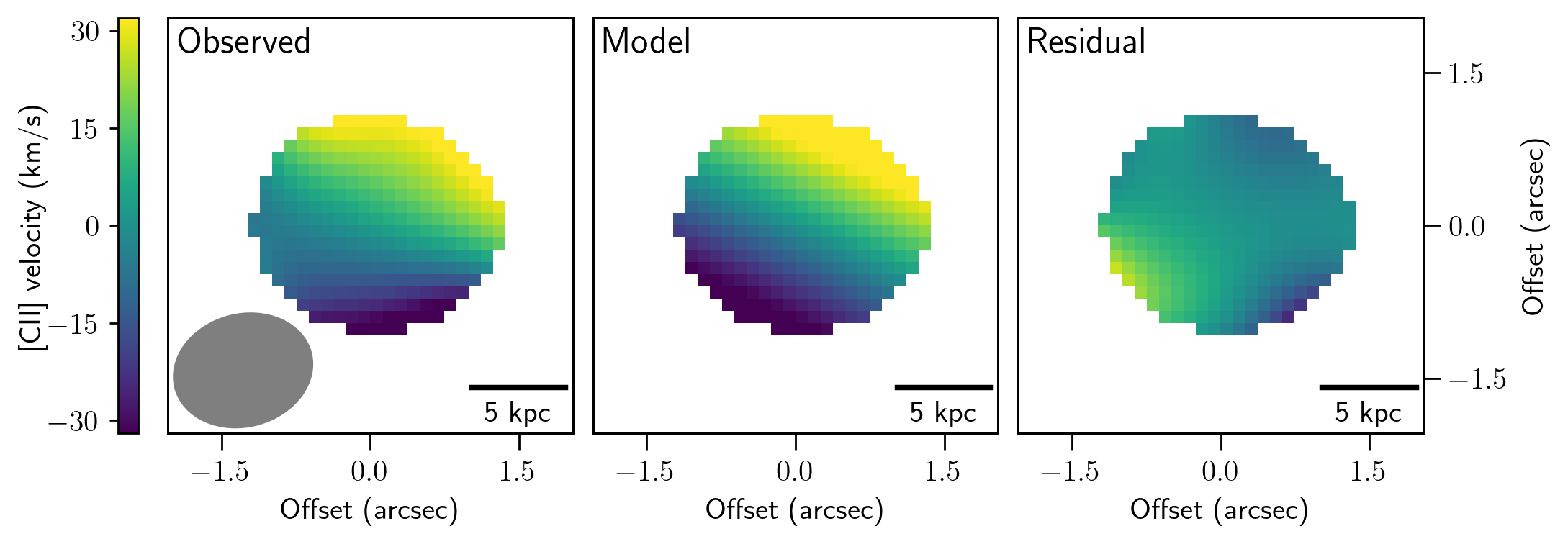
Figure 4: [Left panel] The [Cii] velocity field of REBELS-25 (Schouws et al. in prep.). The beam is shown as a grey ellipse in the bottom left corner of the Left panel and a scale bar showing 5 kpc is displayed in the bottom right corner of each panel. The velocity field exhibits a clear velocity gradient, which is indicative of disc rotation. We display the best-fitting thin disc model in the Middle panel and the residual between the model and the observed first moment map in the Right panel. However, we note that a similar fit with a merger model is statistically indistinguishable from this model.

To visualise the kinematics of REBELS-25, we display a map of the [Cii] velocity field for REBELS-25 in Figure 4. For full details of the maps we refer the reader to Schouws et al. (in prep.), where they are presented. In brief, the map is made by taking the first moment of the image, with a threshold that only includes individual pixels that are above three times the noise level (i.e. $>3\sigma$). The velocity field exhibits a velocity gradient across the galaxy. Such a velocity gradient could be indicative of disc rotation; however, the resolution of the data preclude us from distinguishing between this and other scenarios. Indeed, Schouws et al. (in prep.) fitted kinematic models of a thin, rotating disc shown in Figure 4 and a separate model of an unresolved merger to REBELS-25 and found them to be statistically indistinguishable from one another. Thus, although we cannot definitively conclude on the source of the kinematic profile, both rotating disc and major merger models provide adequate fits to the data.

Indeed, Rizzo et al. (2022) found that good resolution is essential to correctly model the kinematic state of simulated data, with at least three independent resolution elements across the major axis of the beam needed; this criterion is not met by our low-resolution data. It is plausible, especially given the fact that three separate rest-frame UV sources are detected (Stefanon et al., 2019), that the kinematic profile that we observe may be an artefact resulting from beam smearing of the kinematic profiles of separate sources (see Kohandel et al., 2020). Higher resolution observations are necessary in order to distinguish between these scenarios. Finally, we characterise the velocity gradient in REBELS-25 by estimating the FWHM of the [Cii] line from a fit to the main [Cii] emission component with a single Gaussian, which results in a FWHM of $316\pm 15$ ${\rm km~{}s^{-1}}$.

3.3.1 Dynamical mass

We proceed to estimate the dynamical mass, $M_{\rm dyn}$, of REBELS-25. We employ the method outlined in Kohandel et al. (2019) to calculate it as

$$M_{\rm dyn}=2.35\times 10^{9}\mbox{M${}_{\odot}$}{}\left(\frac{1}{\gamma^{2}\sin^{2}{i}}\right)\left(\frac{\rm FWHM}{100~{}\mbox{${\rm km~{}s^{-1}}$}{}}\right)^{2}\frac{R}{\rm kpc},$$ (1)

where the [Cii] FWHM is measured in km s^-1, the radius of the galaxy, $R$, is measured in kpc, $i$ is the inclination of the galaxy and $\gamma$ is a parameter that depends on the physical nature of the source being considered, in particular its structure and kinematics. For REBELS-25, this translates to $M_{\rm dyn}=8.5\pm 1.9\times 10^{10}\gamma^{-2}\sin^{-2}{i}~{}\mbox{M${}_{\odot}$}$, where we take $R$ to be the major axis of the main [Cii] component, as we have assumed that REBELS-25 is inclined. With our estimate of the inclination of the main [Cii] component of REBELS-25 that we obtained from Gaussian fitting of the component in the zeroth moment map (see Section 3.2), $i=\mbox{$56\pm 29$}{}\degr{}$, this translates to a dynamical mass $M_{\rm dyn}$ $=1.2\pm 0.7\times 10^{11}\gamma^{-2}\mbox{M${}_{\odot}$}{}$

Due to the significant uncertainty in REBELS-25’s morphology, the value of $\gamma$ is similarly uncertain. Kohandel et al. (2019) give a range of values for $\gamma$ derived from Althæa, a simulated high-redshift galaxy (Pallottini et al., 2017), with $\gamma$ = 1.78, 2.03, 1.52, when the galaxy is in a spiral disc, disturbed disc, and merger stage, respectively. Although simulated observations of Althæa are made at a slightly lower redshift than REBELS-25 of $z=6$, it has a comparable stellar mass of $\sim 10^{10}~{}\mbox{M${}_{\odot}$}$ and dynamical mass of $\sim 10^{10}~{}\mbox{M${}_{\odot}$}$ (Kohandel et al., 2019). As REBELS-25 could reasonably be a disc in various kinematic states or a merger with the information available given the current resolution of our data, we do not select one value of $\gamma$ and we thus evaluate $M_{\rm dyn}$ for all three values and report $M_{\rm dyn}$ as a range $M_{\rm dyn}=2-8\times 10^{10}\mbox{M${}_{\odot}$}$.

3.4 ISM properties

We use our measurement of the [Cii] luminosity of REBELS-25 (see Section 3.1) to estimate the molecular gas mass, $M_{{\rm H}_{2}}$ in solar masses, of REBELS-25 from the empirical relation calibrated by Zanella et al. (2018),

$$M_{{\rm H}_{2}}=\alpha_{\mbox{[C{\sc ii}]}{}}L_{\mbox{[C{\sc ii}]}{}},$$ (2)

where $L_{\mbox{[C{\sc ii}]}{}}$ is the [Cii] luminosity in solar luminosities and $\alpha_{\mbox{[C{\sc ii}]}{}}=31^{+31}_{-15}\mbox{M${}_{\odot}$}\mbox{L${}_{\odot}$}^{-1}$ is an empirically calibrated conversion factor. From this relation, we calculate a molecular gas mass of $M_{{\rm H}_{2},\mbox{[C{\sc ii}]}{}}=\mbox{$5.1^{+5.1}_{-2.6}\times 10^{10}$}{}~{}\mbox{M${}_{\odot}$}$. We note, however, that this relation was calibrated for galaxies at significantly lower redshift than REBELS-25 and as noted by Zanella et al. (2018) the conditions of the ISM at very high-redshift are most probably different to low-redshift conditions, which may impact the applicability of the relation to REBELS-25. However, an analysis of the molecular gas masses of a sample of galaxies from the ALPINE survey (Le Fèvre et al., 2020; Béthermin et al., 2020; Faisst et al., 2020) between $4.4<z<5.9$ found that the Zanella et al. (2018) relation agreed with those derived from dynamical masses and dust continuum luminosities (Dessauges-Zavadsky et al., 2020). We have adopted $\alpha_{\mbox{[C{\sc ii}]}{}}=31^{+31}_{-15}$, following Zanella et al. (2018), however, we note that there remains significant uncertainty as to the value of $\alpha_{\mbox{[C{\sc ii}]}{}}$, with studies based on observations and simulations finding values between a few (Rizzo et al., 2021) and about a hundred (Madden et al., 2020). Simulations also suggest that low metallicity galaxies in particular may require a lower value of $\alpha_{\mbox{[C{\sc ii}]}{}}$ (Vizgan et al., 2022).

3.5 Star formation

We calculate the total star formation rate for the galaxy using UV to trace unobscured star formation and IR to trace obscured star formation, as

$${\rm SFR}_{\rm tot}=k_{\rm IR}L_{\rm IR}+k_{\rm UV}L_{\nu,\rm UV},$$ (3)

where $k_{\rm IR}=1.2\times 10^{-10}\mbox{M${}_{\odot}$}\mbox{${\rm yr}$}^{-1}\mbox{L${}_{\odot}$}^{-1}$ and $k_{\rm UV}=7.1\times 10^{-10}\mbox{M${}_{\odot}$}\mbox{${\rm yr}$}^{-1}({\rm ergs~{}s^{-1}Hz^{-1}})^{-1}$. These values of $k_{\rm IR}$ and $k_{\rm UV}$ have been adopted for the REBELS sample (Bouwens et al., 2022) and the rationale and calculation of these factors are further discussed by Stefanon et al. (in prep.), Inami et al. (2022) and Topping et al. (2022).

Inami et al. (2022) determine an IR luminosity for REBELS-25 of $L_{\rm IR}=\mbox{$1.5^{+0.8}_{-0.5}\times 10^{12}$}{}$ L_⊙ (for further details see Section 2.3). The UV luminosity of REBELS-25 is calculated from the best-fitting SED-template obtained with EAzY (Brammer et al., 2008) to be $L_{\rm UV}=9\pm 2\times 10^{10}~{}\mbox{L${}_{\odot}$}$ (Stefanon et al. in prep.). This translates to ${\rm SFR}_{\rm tot}=\mbox{$199^{+101}_{-63}$}{}~{}\mbox{M${}_{\odot}$}~{}\mbox{${\rm yr}$}^{-1}$, with ${\rm SFR}_{\rm UV}=\mbox{$14\pm 3$}{}~{}\mbox{M${}_{\odot}$}\mbox{${\rm yr}$}^{-1}$ and ${\rm SFR}_{\rm IR}={\mbox{$185^{+101}_{-63}$}}{}~{}\mbox{M${}_{\odot}$}\mbox{${\rm yr}$}^{-1}$. From this it can be seen that the obscured star formation, as traced by IR emission, dominates the star formation in REBELS-25.

We also make a second calculation of the SFR by using the [Cii] emission. De Looze et al. (2014) calibrated a relationship between the [Cii] luminosity and star formation rate based on a sample of galaxies, which they refer to as their high-redshift sample, $z=0.5-6.6$

$$\log{\rm SFR}_{\mbox{[C{\sc ii}]}{}}=-8.52+1.18\log L_{\mbox{[C{\sc ii}]}{}}+\log C_{\rm Kroupa},$$ (4)

where $C_{\rm Kroupa}=1.08$ is a factor to convert from a Kroupa & Weidner (2003) IMF to a Chabrier (2003) IMF. From this, we calculate ${\rm SFR}_{\mbox{[C{\sc ii}]}{}}=\mbox{$246\pm 35$}{}\mbox{M${}_{\odot}$}{\rm yr}^{-1}$.

Both methods of calculating the star formation broadly indicate that REBELS-25 is undergoing an active phase of star formation in which a large amount of stellar mass is being added. However, the value of ${\rm SFR}_{\mbox{[C{\sc ii}]}{}}$ is slightly ($\sim 1.25$ times) greater than the value of ${\rm SFR}_{\rm tot}$. Although, when additionally taking account of the significant 0.4 dex uncertainty in the fitted relation this value is consistent with our measurement of the SFR from IR and UV. We note in general that calibrations for the SFR at such high redshift are uncertain due to the limited nature of the observations. Moreover, for [Cii] as a tracer of star formation specifically, Carniani et al. (2018) find that the relationship between SFR and $L_{\mbox{[C{\sc ii}]}{}}$ holds in a sample of $z=5.2-7.2$ galaxies, but has significantly increased scatter in comparison to the relation exhibited in local galaxies. Similarly, Schaerer et al. (2020) find that the relationship between SFR and $L_{\mbox{[C{\sc ii}]}{}}$ is valid in the galaxies of the ALPINE sample at redshifts $4.4<z<5.9$, but also with increased scatter compared to the local relation. As discussed by De Looze et al. (2014), the scatter in the relation between SFR and [Cii] luminosity likely results, in large part, from the differing ISM conditions between different galaxies. Indeed, evidence from observations of local galaxies indicates that metallicity, which is uncertain for REBELS-25, particularly affects the fraction of [Cii] emission emanating from neutral and ionised media (Croxall et al., 2017). Therefore, although there is little evidence of evolution in the relation, the increased scatter at higher redshifts disfavours its usage compared to the UV + IR SFR. We thus adopt the SFR as calculated from the UV and IR emission (i.e. ${\rm SFR}_{\rm tot}$) for our further analysis.

We proceed to calculate a molecular gas depletion time, $t_{\rm depl,{\rm H}_{2}}$, for REBELS-25, that is the time it would take for the inferred molecular gas reservoir of REBELS-25 to be depleted assuming a constant star formation rate and no other gain or loss of molecular gas mass. Under these assumptions, $t_{\rm depl,{\rm H}_{2}}=M_{{\rm H}_{2},\mbox{[C{\sc ii}]}{}}/{\rm SFR}_{\rm tot}=\mbox{$0.3^{+0.3}_{-0.2}$}{}$ Gyr. However, as we discuss in Section 3.1 the additional secondary component that is observed in the [Cii] spectrum is evidence for either an outflow of gas, or a merger or inflow of gas. Under the assumption of no other effects, an outflow would lead to faster depletion of the gas reservoir whereas a merging galaxy or inflow of gas would increase REBELS-25’s gas reservoir and lead to a longer depletion time.

3.6 Properties of the secondary [Cii] emission component

As discussed in Section 3.1, we observe an additional emission component in the REBELS-25 spectrum, slightly to the lower frequency-side of the main line component and fit a number of models to the spectrum of the galaxy. The two best-fitting models, shown in Fig 2, model the secondary component as a merger or an outflow. In this section we present the physical properties that can be determined from our two best-fitting models.

3.6.1 Merger model

One natural origin for this secondary emission component is from another galaxy separate to REBELS-25 that may be merging with the main component. We find that the centre of the secondary emission component is spatially coincident (to within 1.5 kpc) with the primary emission component from image-plane fitting (see also Figure 3) and is offset from the primary emission component in velocity space by $\sim 500~{}\mbox{${\rm km~{}s^{-1}}$}{}$. This close association would suggest that the galaxy will merge into the primary emission component of REBELS-25.

From this model, we measure a [Cii] luminosity of $3\pm 1\times 10^{8}$ L_⊙ for this merging galaxy. Using Equation 2, this translates to a molecular gas mass of $9^{+9}_{-5}\times 10^{9}$ M_⊙, or about 18 per cent the mass of REBELS-25’s molecular gas reservoir. If we assume that the total mass of the galaxies are proportional to their molecular gas reservoirs that we measure from [Cii], this would classify this as a minor merger according to the commonly used definition of a minor merger as one where the mass ratio between the two galaxies is 1:3 or greater, however, we note that there can be significant differences between the ratios of total mass and the mass ratios of individual components of a galaxy (Stewart, 2009). Although only a minor merger, this would still serve to increase the amount of molecular gas in REBELS-25’s reservoir and thus the galaxy’s potential future stellar mass.

3.6.2 Outflow model

Another plausible origin for the secondary emission component is from an outflow. We follow the method outlined by Herrera-Camus et al. (2021) to estimate the properties of our best-fitting outflow model. The atomic hydrogen outflow rate $\dot{M}_{\rm H{\sc I},out}$, can be estimated as

$$\dot{M}_{\rm H{\sc I},out}=M_{\rm H{\sc I},out}\left(\frac{v_{\rm out}}{R_{\rm out}}\right),$$ (5)

where $M_{\rm H{\sc I},out}$ is the atomic hydrogen mass of the outflow, $v_{\rm out}$ is the velocity of the outflow and $R_{\rm out}$ is the size of the outflow.

Following Herrera-Camus et al. (2021), we first calculate an estimate of the projected outflow velocity, $v_{\rm out,proj}$, as

$$v_{\rm out,proj}\sim\left|\Delta v\right|+\frac{FW_{10\%}}{2},$$ (6)

where $\Delta v$ is the difference in velocity between the outflow and the main component and $FW_{10\%}$ is the full width at tenth maximum of the outflow component. The best-fitting outflow component of our model has a $FW_{10\%}=1600\pm 400\mbox{${\rm km~{}s^{-1}}$}{}$ and is separated from the main [Cii] emission component by $\left|\Delta v\right|=100\pm 80$ ${\rm km~{}s^{-1}}$, which translates to a projected outflow velocity of $900\pm 200$ ${\rm km~{}s^{-1}}$.

Under the assumption of an outflow perpendicular to the assumed disc of REBELS-25, we can use our estimate of the inclination of the main [Cii] component, $i=\mbox{$56\pm 29$}{}\degr{}$ to further estimate the deprojected outflow velocity as $v_{\rm out,deproj}=v_{\rm out}/\cos{i}=1600\pm 300$ ${\rm km~{}s^{-1}}$.

Herrera-Camus et al. (2021) presented a relationship between atomic hydrogen mass in the outflow, $M_{\rm H{\sc I},out}$ and the [Cii] luminosity under the assumption that the collisional excitation of $\rm C^{+}$ is primarily due to hydrogen atoms:

$$M_{\rm H{\sc I},out}=\kappa_{\scriptsize\mbox{[C{\sc ii}]}{}}L_{\scriptsize\mbox{[C{\sc ii}]}{}},$$ (7)

where $\kappa_{\mbox{[C{\sc ii}]}{}}$ is a conversion factor dependant on the temperature, metallicity and number density of atomic hydrogen gas. We calculate a lower limit to the atomic gas mass under the “maximal excitation conditions” scenario presented by Herrera-Camus et al. (2021), with $\kappa_{\mbox{[C{\sc ii}]}{}}=1.5~{}\mbox{M${}_{\odot}$}/\mbox{L${}_{\odot}$}$. This value of $\kappa_{\mbox{[C{\sc ii}]}{}}$ is calculated by assuming a Helium fraction of 36%, solar metallicity, a temperature of $10^{4}$ K and number density of $10^{4}~{}{\rm cm}^{-3}$ for the gas. We determine a [Cii] luminosity of $7\pm 3$ $\times 10^{8}$ L_⊙ for the outflow component of our best-fitting model, which translates to an estimated lower limit of $M_{\rm H{\sc I},out}$ $\gtrsim 1.1\times 10^{9}$ M_⊙.

We have chosen to use the “maximal excitation conditions” scenario presented by Herrera-Camus et al. (2021) in order to provide a conservative estimated lower limit of the outflow mass. However, we note that the true physical conditions of the gas may well be different to those that we have considered. In particular, although measurements of the metallicity of high redshift galaxies are limited, subsolar metallicities are considered to be most likely (see reviews by Stark, 2016; Dayal & Ferrara, 2018). With the other conditions kept the same, a subsolar metallicity would lead to an increase of$\kappa_{\mbox{[C{\sc ii}]}{}}$ to $4.7~{}\mbox{M${}_{\odot}$}/\mbox{L${}_{\odot}$}$ in the case of half solar metallicity and $41.7~{}\mbox{M${}_{\odot}$}/\mbox{L${}_{\odot}$}$ in the case of metallicity one tenth of solar metallicity (for the details of the calculation of these values of $\kappa_{\mbox{[C{\sc ii}]}{}}$ see Herrera-Camus et al., 2021). This would lead to a corresponding increase in our estimate of the lower limit of the outflow mass by a factor of $\sim 3$ for half solar metallicity and a factor of $\sim 30$ in the case of one tenth solar metallicity. In order to provide a better estimate of the outflow mass, multi-line observations of REBELS-25 are required to obtain an accurate estimate of the metallicity.

Last, we use the average of the major and minor axes of our image plane fit to the outflow component (see Section 3.2) to estimate $R_{\rm out}\approx 9$ kpc. We then combine our estimates of $M_{\rm H{\sc I},out}$, $v_{\rm out}$ and $R_{\rm out}$ to derive an estimated lower limit of the projected atomic mass outflow rate of $\dot{M}_{\rm out,proj}\gtrsim 120$ M_⊙ $\mbox{${\rm yr}$}^{-1}$, and an estimated lower limit of the deprojected atomic mass outflow rate $\dot{M}_{\rm out,deproj}\gtrsim\mbox{$200$}{}$ M_⊙ $\mbox{${\rm yr}$}^{-1}$. From these outflow rates we estimate a lower limit of the atomic mass loading factor, $\lambda=\dot{M}_{\rm out}/{\rm SFR}$. We estimate a projected mass loading factor of $\lambda_{\rm proj}\gtrsim 0.6$ and a deprojected mass loading factor of $\lambda_{\rm deproj}\gtrsim 1.0$. In other words we estimate a project lower limit that is roughly half the SFR of REBELS-25 and a deprojected lower limit that is roughly equivalent to this SFR.

4 Discussion

4.1 The Nature of REBELS-25

We discuss here the nature of REBELS-25 in the context of the observational results that we have presented in Section 3 and results from the literature.

4.1.1 ULIRG

REBELS-25 is notable for its significant IR emission ($L_{\rm IR}=\mbox{$1.5^{+0.8}_{-0.5}\times 10^{12}$}{}$ L_⊙), making it the only ULIRG in the REBELS sample (see Figure 1). If the ISM conditions that we have adopted in order to determine the IR luminosity deviate from the true ISM conditions of REBELS-25, this will in turn impact our estimate of the IR luminosity. In particular, we have adopted the median dust temperature (46K) determined from a sample of the REBELS galaxies (see Section 2.3 for further details). Direct determinations of the dust temperature by SED fitting in galaxies at a redshift comparable to REBELS-25 are limited by the lack of sources with observations at higher frequency than the dust emission peak. However, the temperature that we adopt is comparable to the temperature of $42^{+13}_{-7}$K measured for a less IR luminous ($\sim 2\times 10^{11}\mbox{L${}_{\odot}$}{}$) galaxy at $z=7.13$ that has such observations (Bakx et al., 2021).

There have now been two works that attempt to determine the dust temperature and IR luminosity of REBELS-25 in the absence of a well-sampled dust SED. Using their method combining a single dust continuum measurement with a [Cii] line luminosity, Sommovigo et al. (2022a) determine an even higher dust temperature ($55^{+15}_{-14}$K, corresponding to an IR luminosity of $\log{L_{\rm IR}}=12.45^{+0.43}_{-0.45}\mbox{L${}_{\odot}$}$) than that which we have adopted. Meanwhile, using an additional ALMA Band 8 observation of REBELS-25, Algera et al. (2023a) fit an SED to the two observed continuum fluxes. In their fiducial optically thin model with a dust emissivity index $\beta=2.0$, they determine a lower dust temperature of $34^{+6}_{-6}$K and a corresponding IR luminosity of $\log{L_{\rm IR}}=11.85^{+0.18}_{-0.10}\mbox{L${}_{\odot}$}$. However, when modifying their fiducial model by instead adopting $\beta=1.5$ or fitting for $\beta$, they determine temperatures of $43^{+11}_{-8}$K and $42^{+24}_{-11}$K, corresponding to IR luminosities of $\log{L_{\rm IR}}=12.02^{+0.28}_{-0.20}\mbox{L${}_{\odot}$}$ and $\log{L_{\rm IR}}=12.00^{+0.46}_{-0.22}\mbox{L${}_{\odot}$}$, respectively. They find even higher values for the dust temperature and IR luminosity in the optically thick scenarios compared to the corresponding optically thin scenarios.

Given its probable status as a ULIRG, the question arises as to whether REBELS-25 has different dust properties to the rest of the REBELS sample and what impact this may have on the IR luminosity. Sommovigo et al. (2022b) find that the ULIRGs in the sample of ALPINE galaxies that they analyse have higher dust temperatures than the other galaxies. However, the other conditions of the dust, in particular the dust emissivity index, play an important role, as seen above. Observations of ULIRGs in the Local Universe (Clements et al., 2018) and $z~{}\sim~{}1-3$ submm galaxies (da Cunha et al., 2021) indicates that there is a general correlation between higher dust temperature and higher IR luminosity for high IR luminosity galaxies (including ULIRGs). Furthermore, observations of nearby galaxies (Lamperti et al., 2019) and $z~{}\sim~{}1-3$ submm galaxies (da Cunha et al., 2021) show a correlation between higher dust temperature and lower dust emissivity index. If these trends are also present in the Epoch of Reionisation then this would further support a higher IR luminosity for REBELS-25, in the case that we have adopted a lower dust temperature than the true value. If we have underestimated the IR luminosity of REBELS-25, we would have consequently underestimated the obscured (and thus total) SFR. To conclusively determine the IR luminosity of REBELS-25 and thus its SFR, high frequency observations of REBELS-25 that well-sample the dust SED are required.

Recent work by Zavala et al. (2021) to constrain the IR luminosity function, suggests that ULIRGs should make the dominant contribution to the total obscured star formation rate at the redshift covered by the REBELS sample. However, the other (non-ULIRG) galaxies in the REBELS sample account for the majority of the obscured star formation in the REBELS sample (Inami et al., 2022). It is possible, however, that this discrepancy is explained by the design of the REBELS survey. The REBELS survey selected galaxies on the basis of UV observations (Bouwens et al., 2022) and thus may be prone to disproportionately select dust-poorer galaxies for observation, which are less likely to have significant IR luminosities in comparison to the population of galaxies as a whole. Indeed this scenario is also a possible explanation for the tension between the dust masses of the REBELS sample and the UV luminosity function (for further discussion see Dayal et al., 2022). This scenario is supported by the finding of Sommovigo et al. (2022a) who present an analytical model of the evolution of dust temperature with redshift and find that the dust temperature of the REBELS galaxies is typical of quite UV-transparent galaxies in the context of this model.

Furthermore, the IR luminosities of the REBELS galaxies presented by Inami et al. (2022) and used in this paper are calculated by converting a monochromatic luminosity to a total IR luminosity. There is of course uncertainty inherent in this conversion, including from the uncertainty in the dust temperature (see discussion in Sommovigo et al., 2022a). It is possible that a more-thorough determination of their IR luminosities from observations that sample the IR luminosity distribution at multiple wavelengths would result in a greater fraction of the REBELS galaxies being classified as ULIRGs. The evidence from other approaches to constrain the IR luminosity is mixed, however. Sommovigo et al. (2022a) used a model to predict the IR luminosities of a subsample of thirteen of the REBELS galaxies using both their monochromatic continuum luminosities and [Cii] line luminosities; they predict REBELS-25 to be the only ULIRG in the subsample. Ferrara et al. (2022) used UV continuum flux, the UV spectral slope and the monochromatic continuum luminosity of the REBELS galaxies in combination with radiative transfer models using different simple geometries to derive IR luminosities of the sample; for a Milky Way extinction curve, they find two other galaxies in the REBELS sample that have IR luminosities above $10^{12}$ L_⊙. However, for an SMC extinction curve they find IR luminosities below $10^{12}$ L_⊙ for both galaxies. We note that Ferrara et al. (2022) could not determine an IR luminosity for REBELS-25, due to its very high dust-continuum flux, which is consistent with it being very IR luminous in comparison to the REBELS sample.

4.1.2 Morphology

Our observations indicate a morphologically complex nature for REBELS-25. The spectrum of REBELS-25 includes a faint [Cii] emission component, spectrally-separated from the main [Cii] emission component (See Figure 2), which we have interpreted as being potential evidence of a minor merger or an outflow (see Section 3.1). Although there are still limited constraints on the frequency of mergers at high redshift, they appear somewhat common, but less frequent than at intermediate redshifts. A recent analysis also suggests that the fraction of minor mergers decreases towards higher redshift after peaking at intermediate redshift, with the fraction of minor mergers being 8-13 per cent at $z\geq 3$ (Ventou et al., 2019), consistent with prior analyses that indicate that the fraction of major mergers decrease at higher redshift (Xu et al., 2012; Ventou et al., 2017, 2019). Le Fèvre et al. (2020) found that 40 per cent of galaxies in the ALPINE sample of galaxies at $4<z<6$ were mergers with a subsequent analysis combining the ALPINE survey with lower redshift samples by Romano et al. (2021) indicating that the peak of the major merger rate is at $z\sim 3$ and slowly declines towards higher redshifts, with a major merger frequency of 34 per cent at $z\sim 5.5$. Star-formation-driven outflows have also been detected at high redshift (e.g. Herrera-Camus et al., 2021), though statistics on their frequency remain somewhat scant. Theoretical results suggest, however, that [Cii] haloes can be explained by prior outflows (Pizzati et al., 2020), which would provide evidence that they are common at this redshift. We explore the observational context for and implications of an outflow further in Section 4.3, but note that both scenarios are plausible.

Prior analysis of rest-frame UV imaging identified multiple UV components at the location of REBELS-25 (Stefanon et al., 2019) and a prior study found dust continuum emission offset from these UV components (Schouws et al., 2022a). We observe an offset between this UV emission and both the centres of the [Cii] and dust continuum emission in REBELS-25 (see Figure 3). In addition, Ferrara et al. (2022) finds that REBELS-25 has a much larger ratio of dust continuum flux to UV continuum flux than would be expected from its UV spectral slope, which is indicative of UV and IR emission emanating from spatially decoupled regions. Offsets between the UV and dust emission in galaxies have been commonly observed in lower-redshift SMGs and may indicate a physical offset between the dust and the sites of star formation, for example due to the morphological disturbance of a merger or may instead suggest that the UV clumps are embedded in a larger dusty galaxy and are visible due to reduced attenuation from dust at their location (Hodge et al., 2015, 2016; Chen et al., 2017; Calistro Rivera et al., 2018; Hodge et al., 2019; Rujopakarn et al., 2019; Cochrane et al., 2021). At high-z, offsets between [Cii] and UV emission have also been observed. Maiolino et al. (2015) found such an offset in three $z\sim 7$ galaxies and they attributed the lack of [Cii] emission in the vicinity of the UV emission to molecular clouds being dispersed by stellar feedback on short timescales. Although the observed offset between the centre of the [Cii] emission and the UV emission components could hint at a similar scenario in REBELS-25, the large beam of our current [Cii] data means that it is not possible to determine whether or not there is [Cii] emission coincident with the UV emission. Fujimoto et al. (2020) measured offsets between the UV and both the [Cii] and dust continuum for the galaxies of the ALPINE sample at $4<z<6$. For those galaxies not identified as mergers, they were unable to determine whether the observed offsets were physical or a result only of astrometric and positional uncertainty. More recently, two studies have examined the frequency of offsets between dust and UV emission in the EoR. Schouws et al. (2022a) found that the dust and UV were co-spatial in the majority of the six galaxies at $z\sim 7-8$ that they detected in dust, with the exception of REBELS-25, for which they observed an offset. Bowler et al. (2022) found that three out of a sample of six bright galaxies at $z\sim 7$ with high resolution ALMA imaging have a significant dust detection that is offset from the galaxy’s UV emission. Offsets between the dust continuum emission and UV are explored for the REBELS sample in Inami et al. (2022), who find additional galaxies within the sample that exhibit offsets. Thus the picture at high-z remains somewhat unclear, but initial results suggest that offsets between dust and other components are somewhat common in bright galaxies at high redshift.

4.1.3 Kinematics

We observe a significant velocity gradient in the main [Cii] emission component of REBELS-25 (see Figure 4), which may be indicative of a rotating disc. However, with the large size of the beam of our observations, the observed velocity gradient could also be produced by beam smearing of merging galaxies. As discussed above, mergers are not uncommon at high redshift. It is unclear, however, how common rotating discs are at such high redshifts. The conventional model of disc formation in galaxies, has discs forming through the process of cooling and dissipation (see e.g Eggen et al., 1962; Rees & Ostriker, 1977; White & Rees, 1978; Fall & Efstathiou, 1980), which results in the formation of discs at relatively late times, roughly around the time of cosmic noon. However, signatures of rotating discs have been observed out to higher and higher redshifts $z>4-5$ (see e.g. Smit et al., 2018; Pavesi et al., 2019; Bakx et al., 2020; Rizzo et al., 2020; Neeleman et al., 2020; Jones et al., 2021; Lelli et al., 2021). Indeed, in a study of the kinematics of high-z ($z\gtrsim 6$) quasar host galaxies, Neeleman et al. (2021) found ten out of the 27 studied galaxies have a rotational profile consistent with that of a rotating gas disc. In addition, from the perspective of theory, modern, hydrodynamical simulations also are able to produce a significant fraction of disc galaxies at redshifts well-above cosmic noon (e.g. Pallottini et al., 2017; Pallottini et al., 2019; Pillepich et al., 2019; Leung et al., 2020; Kohandel et al., 2020).

Overall, the observational evidence indicates that REBELS-25 is a morphologically complex galaxy, potentially comprising some combination of a rotating disc, merging galaxies and outflowing gas. In addition, REBELS-25 is observed to have significant stellar, gas and dust mass components built up at a high redshift. However, further multi-wavelength and higher resolution observations are required to resolve the uncertainties in the morphology and composition of the galaxy.

4.2 Main sequence comparison

We can compare the star formation properties of REBELS-25 to the star formation main sequence of Speagle et al. (2014) and the relation for $t_{\rm depl,{\rm H}_{2}}$ of Liu et al. (2019). We note, however, that as both Liu et al. (2019) and Speagle et al. (2014) based their studies on data out to redshift $z\sim 6$, our application of these relations represents an extrapolation of these data under the assumption that the trends observed out to $z\sim 6$ will continue to hold at higher redshift, which may not be valid.

The best-fitting main-sequence of Speagle et al. (2014) is

$$\log{{\rm SFR}_{\rm MS}}=(0.84-0.026t_{\rm age})\log{M_{*}}-(6.51-0.11t_{\rm age}),$$ (8)

where $t_{\rm age}$ is the age of the universe in Gyr, which at $z\sim 7.31{}$ is 0.71 Gyr with our adopted cosmology. For the stellar mass of REBELS-25 (see Section 2.3) this translates to a prediction of ${\rm SFR}_{\rm MS}=\mbox{$49$}{}~{}$ M_⊙yr^-1. The total SFR that we measure for REBELS-25 of $\mbox{$199^{+101}_{-63}$}{}~{}\mbox{M${}_{\odot}$}\mbox{${\rm yr}$}^{-1}$ is approximately four times this main-sequence value of Speagle et al. (2014). If we instead take the larger non-parametric stellar mass estimate, this would translate to a prediction of $101$ M_⊙yr^-1, placing REBELS-25’s SFR at about twice the main-sequence value. Topping et al. (2022) use the REBELS sample to determine a high-redshift main-sequence by fixing the slope of the main-sequence to that presented by Speagle et al. (2014) and selecting the best-fitting intercept. The main sequence presented by Topping et al. (2022) was determined using a non-parametric method to determine stellar mass. If we adopt the same approach as Topping et al. (2022), but instead use stellar masses for the REBELS sample that have been determined by assuming a constant star formation history, as adopted in this paper, we determine a main sequence of the form

$$\log{{\rm SFR}_{\rm T22}}=0.82\log{M_{*}}-5.93.$$ (9)

Using this prescription would result in a higher main sequence SFR of ${\rm SFR}_{\rm T22}$ $\sim 151$ M_⊙yr^-1. REBELS-25’s SFR is comparable to (1.3 times) this predicted value.

Khusanova et al. (2021) presented a main sequence derived from the ALPINE survey of galaxies. We consider the main sequence presented for galaxies at $z~{}\sim 5.5$, which is the higher redshift of the two main sequences presented by Khusanova et al. (2021). This main sequence has the form

$$\log{{\rm SFR}_{\rm K21}}=0.66\log{M_{*}}-5.1$$ (10)

(Khusanova et al. 2021; Khusanova, private communication). Using this prescription would result in a lower main sequence star formation rate of ${\rm SFR}_{\rm K21}\sim 27$ M_⊙yr^-1 with our adopted stellar mass. In comparison REBELS-25’s SFR is $\sim 7$ times this value. If we instead use the non-parametric stellar mass of REBELS-25 this would result in a main sequence SFR of $\sim 48$ M_⊙yr^-1, placing REBELS-25 $\sim 4$ times above this main sequence value.

Although there is no consensus regarding the definition of a starburst galaxy, a simple definition is a threshold based on a multiple of the main-sequence-predicted star formation rate. For example, if we take a threshold of three times in excess of that predicted by the main-sequence (see e.g. Elbaz et al., 2018), this places REBELS-25 on the threshold for a starbursting galaxy if we adopt the Speagle et al. (2014) main sequence with our adopted stellar mass. However, given the range of star-forming main sequences and starburst definitions that could be adopted, such a classification must be seen as very tentative. Indeed, if we were to take the main sequence of Equation 9, or the non-parametric stellar mass presented by Topping et al. (2022), REBELS-25 would be classified as a main sequence galaxy. In further contrast, if we take the main sequence prescription of Khusanova et al. (2021), this would place REBELS-25 clearly in the starburst regime for both our adopted stellar mass and the non-parametric stellar mass.

Sommovigo et al. (2022a) determined a dust mass of $4^{+4}_{-1}\times 10^{7}~{}\mbox{M${}_{\odot}$}{}$ for REBELS-25, with a higher dust temperature and infrared luminosity than that adopted in this paper. This would correspond to a dust-to-gas ratio of 0.0007. If we use the same dust model as Sommovigo et al. (2022a), but compute the dust mass with $T_{\rm dust}=46$ K and $L_{\rm IR}=\mbox{$1.5^{+0.8}_{-0.5}\times 10^{12}$}{}~{}\mbox{M${}_{\odot}$}$, as used throughout this paper, we would determine a lower dust mass of $\sim 2\times 10^{7}~{}\mbox{M${}_{\odot}$}{}$, which would correspond to a dust-to-gas ratio of 0.0004. The dust-to-gas ratio is strongly metallicity dependent in nearby galaxies (see e.g. Leroy et al., 2011; De Vis et al., 2019), thus follow up observations to obtain a reliable measurement of the metallicity in REBELS-25 and other galaxies in the EoR would enable REBELS-25 to be placed in context.

Compared to local star-forming galaxies, which have a molecular gas depletion time of about $\sim 2$ Gyr (Bigiel et al., 2008; Bigiel et al., 2011), REBELS-25 has a much shorter molecular gas depletion time of $t_{\rm depl,{\rm H}_{2}}=\mbox{$0.3^{+0.3}_{-0.2}$}{}$ Gyr. Such comparatively short depletion times are common in high-z galaxies (see e.g. review by Hodge & da Cunha, 2020). We calculate a predicted main-sequence depletion time of 0.53 Gyr based on the prescription of Liu et al. (2019). Our inferred value of $t_{\rm depl,{\rm H}_{2}}$ is about one half of this predicted value, which is slightly longer than would be predicted from the enhanced SFR of REBELS-25, suggesting REBELS-25 also has a more massive gas reservoir than would be predicted by the main sequence.

4.3 Implications of a potential outflow

Outflows have been inferred from [Cii] in AGN host galaxies at a similar redshift as REBELS-25 (Maiolino et al., 2012; Cicone et al., 2015; Izumi et al., 2021) and in star-forming galaxies at lower $4<z<6$ redshift (Gallerani et al., 2018; Ginolfi et al., 2020b; Herrera-Camus et al., 2021). Moreover, observations with other tracers indicate they are a common feature at high redshift, with 73 per cent of a sample of eleven lensed dusty star forming galaxies observed having a detected outflow (Spilker et al., 2020a). Outflows can transport material away from their host galaxies and thus can contribute to quenching star formation if the material escapes the galaxy. Modelling of observations indicates that outflows are a necessary component to explain observed quenching (Trussler et al., 2020). They may also be the origin of [Cii] haloes around galaxies (Pizzati et al., 2020). They thus plays an important role in shaping the evolution of galaxies. If REBELS-25 has a sustained outflow over a long period, this would serve to reduce the gas available to form stars and thus the potential for REBELS-25 to accumulate stellar mass.

Observations in the Local Universe find that star formation-driven outflows typically have mass loading factors $\lesssim 4$, whereas AGN-driven outflows can have much higher mass loading factors (see e.g. Cicone et al., 2014; Fluetsch et al., 2019). Although observations of star-formation driven outflows at high-z are much more limited in comparison they typically find similarly low mass loading factors (see e.g. Ginolfi et al., 2020a; Spilker et al., 2020a; Herrera-Camus et al., 2021).

In Section 3.6.2, we estimated a lower limit on the mass loading factor of 0.6 (projected) and 1.0 (deprojected). A mass outflow rate slightly below the SFR (the projected lower limit) or roughly equivalent to it (the deprojected lower limit) would be consistent with a star-formation driven outflow. However, a large uncertainty in the determination of the mass loading factor is the size of the outflow. For these estimates, we adopted a size of 9 kpc based on our image plane fitting. However, it may be that the true size of the outflow is smaller. If we instead adopted a value of $R_{\rm out}=6$ kpc, as was used by Ginolfi et al. (2020a), this would result in a projected mass loading factor of 0.8 and a deprojected mass loading factor of 1.5. In other words an outflow rate that is comparable to or slightly above the star formation rate. Instead adopting $R_{\rm out}=2$ kpc, as was determined for an outflow by Herrera-Camus et al. (2021) with higher resolution observations, would result in a projected mass loading factor of 2.5 and a deprojected mass loading factor of 4.4. In other words, an outflow rate that is significantly in excess of the star formation rate and pushing towards values more comparable to mass loading factors observed in AGN-driven outflows (see e.g. Cicone et al., 2014; Fluetsch et al., 2019). Evidence from local galaxies indicates that outflows typically have a total mass outflow rate about three times that of the atomic mass component for star formation driven outflows and two times as much for AGN-driven outflows (Fluetsch et al., 2019). If the relationship observed by Fluetsch et al. (2019) holds at high redshift, our largest estimates of the total outflow rate would be outside the $1\sigma$ range of observations from local star-formation driven outflows, for the lower end of our star formation estimate for REBELS-25. However, the majority of our estimate range is consistent with the properties of local star formation-driven outflows. We display the range of mass outflow rates that we estimate with the above considerations, in comparison to a number of literature sources in Figure 5. Further work is needed to characterise star-formation driven outflows at high redshift to better understand their properties in comparison to those in the Local Universe.

We also compare our results to the predictions of the delphi semi-analytic model for galaxy formation (Dayal et al., 2014; Dayal et al., 2022). In brief, delphi uses a binary merger tree approach to jointly track the build-up of dark matter halos and their baryonic components (gas, stellar, metal and dust mass). The model follows the assembly histories of $z\sim 4.5$ galaxies with halo masses ${\rm log}(M_{h}/\mbox{M${}_{\odot}$})=8-14$ up to $z\sim 40$. The model contains only two mass- and redshift-independent free parameters, which are tuned to simultaneously reproduce the observed stellar mass function and the UV luminosity function at $z\sim 5-12$. These two parameters are the maximum (instantaneous) star formation efficiency (8 per cent) and the fraction of the type II supernova explosion energy (7.5 per cent) that is available to drive an outflow. For the full details of the physics underpinning the model we refer the reader to Dayal et al. (2014) and Dayal et al. (2022).

For galaxies with ${\rm SFR}>1~{}\mbox{M${}_{\odot}$}~{}{\rm yr^{-1}}$ the delphi model yields an outflow rate ($\dot{M}_{\rm out}$) that scales with SFR as

$$\log\dot{M}_{\rm out}=0.068~{}\log\left({\rm SFR}^{2}\right)+0.59~{}\log\left({\rm SFR}\right)+0.61.$$ (11)

For REBELS-25’s SFR of $\mbox{$199^{+101}_{-63}$}{}~{}\mbox{M${}_{\odot}$}~{}{\rm yr^{-1}}$ , this model would yield an outflow rate of $190^{+65}_{-45}~{}\mbox{M${}_{\odot}$}~{}{\rm yr^{-1}}$. This prediction lies within the region of our observational estimate, which we display in Figure 5 and is in good agreement with our observational estimate of the lower limit of the outflow rate of $\dot{M}_{\rm out,deproj}\gtrsim\mbox{$200$}{}$ M_⊙ $\mbox{${\rm yr}$}^{-1}$.

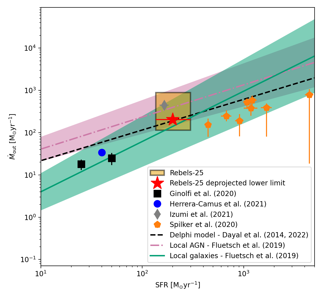
Figure 5: The outflow mass flow rate $\dot{M}_{\rm out}$ against the SFR for REBELS-25 and other sources from the literature. We indicate the deprojected lower limit of $\dot{M}_{\rm out}$ for REBELS-25 with a red star, and we indicate the range of uncertainty as an orange rectangle with a black outline. The outflow properties of a $z\sim 5.5$ galaxy (Herrera-Camus et al., 2021) are shown as a blue circle without errors, as it is reported as an estimate. Outflow properties from a sample of $z>4$ dusty star forming galaxies (Spilker et al., 2020b) are shown as orange pentagons with errors. The outflow properties measured from a stacking analysis of galaxies at $4<z<6$ (Ginolfi et al., 2020a) are show as black squares with errors. An outflow from a $z\sim 7$ AGN (Izumi et al., 2021) is shown as a grey diamond with errors on the SFR, but none on $\dot{M}_{\rm out}$, as this is reported as an estimate. The prediction of the delphi semi-analytic model (Dayal et al., 2014; Dayal et al., 2022) is shown as a black dashed line. Scaling relations from Fluetsch et al. (2019), which we have partially extrapolated beyond the highest SFR values probed in the Fluetsch et al. (2019) sample, are shown for the outflow rate of local AGN-driven outflows (pink dot-dashed line and pink shaded area) and for the outflow rate of local star-forming galaxy driven outflows (solid green line and green-shaded area). Overall, the majority of the range of $\dot{M}_{\rm out}$ we estimate is consistent with local star-formation driven outflows, but the upper range of our $\dot{M}_{\rm out}$ estimate is more comparable to local AGN-driven outflows.

4.4 The fate of REBELS-25

Given its large stellar mass ($M_{*}=\mbox{$8^{+4}_{-2}\times 10^{9}$}{}~{}\mbox{M${}_{\odot}$}{}$), large molecular reservoir ($5.1^{+5.1}_{-2.6}\times 10^{10}$ M_⊙), high SFR ($\mbox{$199^{+101}_{-63}$}{}~{}\mbox{M${}_{\odot}$}~{}\mbox{${\rm yr}$}^{-1}$) at a redshift of $z=7.31{}$, one can ask whether REBELS-25 could evolve into a galaxy similar to massive high-redshift quiescent galaxies, such as those observed by recent studies (Glazebrook et al., 2017; Schreiber et al., 2018b; Merlin et al., 2019; Carnall et al., 2020; Forrest et al., 2020a, b; Saracco et al., 2020; Tanaka et al., 2019; Valentino et al., 2020; Kubo et al., 2021) with stellar masses $\log M_{*}\gtrsim 10.5$ and significantly sub-main-sequence SFRs.

Indeed, if we assume that REBELS-25 continues to form stars at its current rate with no other gain or loss of molecular gas and that it converts 100 per cent of its gas reservoir into stellar mass, REBELS-25 would deplete its molecular gas by $z\sim 5.8$ and have a total stellar mass of $\log\left(M_{*}/\mbox{M${}_{\odot}$}\right)=10.8$. This simple analysis suggests that REBELS-25 has the required molecular gas to obtain a stellar mass consistent with those of the recently observed high-redshift quiescent galaxies by $z\sim 4$. However, the assumption of a constant SFR is unrealistic due to the very high star formation efficiency this would require at later times (without replenishment of the gas reservoir). Furthermore, observational evidence suggests that outflows are common in high-z dusty galaxies (see e.g. Spilker et al., 2020a) and we observe the potential signature of an outflow in REBELS-25 (see Section 3.6.2).

We note that we have conservatively adopted a stellar mass of $M_{*}=\mbox{$8^{+4}_{-2}\times 10^{9}$}{}\mbox{M${}_{\odot}$}{}$ for this analysis, as throughout the paper. However, if we instead adopted the higher non-parametric stellar mass of $19^{+5}_{-8}\times 10^{9}$ M_⊙ for this analysis, this would serve to slightly increase the model’s predicted stellar mass for REBELS-25, but would not qualitatively alter our result.

In this section, we investigate the feasibility of this scenario by considering a simple, conservative evolutionary model in which REBELS-25 evolves with only its current gas reservoir.

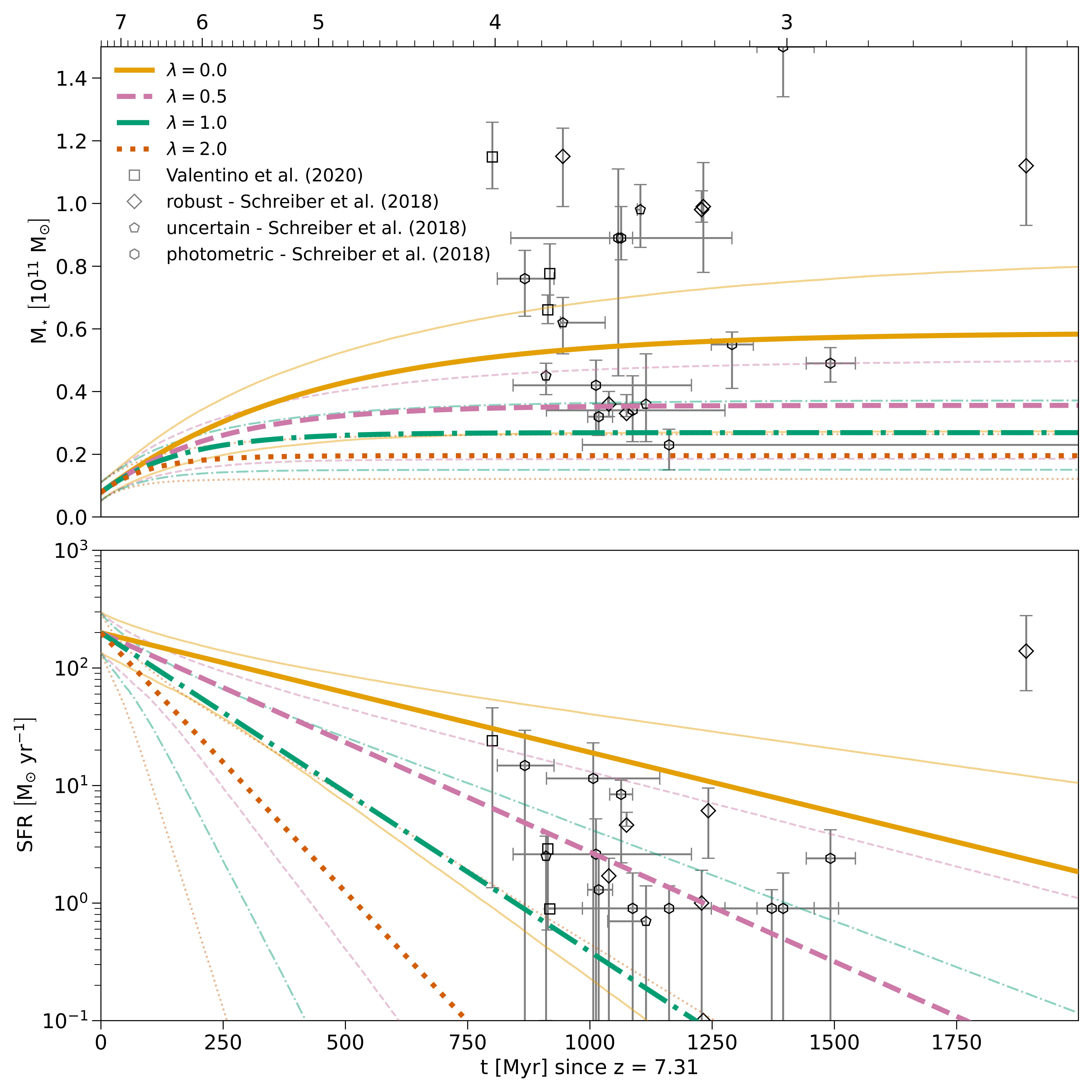
Figure 6: The predicted evolution of the stellar mass [Top panel] and SFR [Bottom panel] for REBELS-25 derived from a simple conservative model under the assumption of continuous star formation with constant star formation efficiency and no inflow of gas. We consider four different scenarios for a continuous gas outflow with mass loading factors of 0 (yellow solid evolution track, equivalent to no outflow), 0.5 (pink dashed evolution track), 1 (teal dot-dashed evolution track) and 2 (red dotted evolution track). For each evolutionary track, the thick opaque line shows the evolutionary track for the properties of REBELS-25 measured in this paper and the two thin semi-transparent lines indicate the region bounded by the 16th and 84th percentiles of the SFR and stellar mass distributions from a sample of evolutionary tracks with starting conditions randomly selected from the uncertainty distributions of these parameters. The SFRs and stellar masses of observed high-z quiescent galaxies are indicated on the plot as open squares (Valentino et al., 2020), open diamonds (the robust spectroscopic sample of Schreiber et al., 2018b), open pentagons (the uncertain spectroscopic sample of Schreiber et al., 2018b) and open hexagons (the photometric sample of Schreiber et al., 2018b).

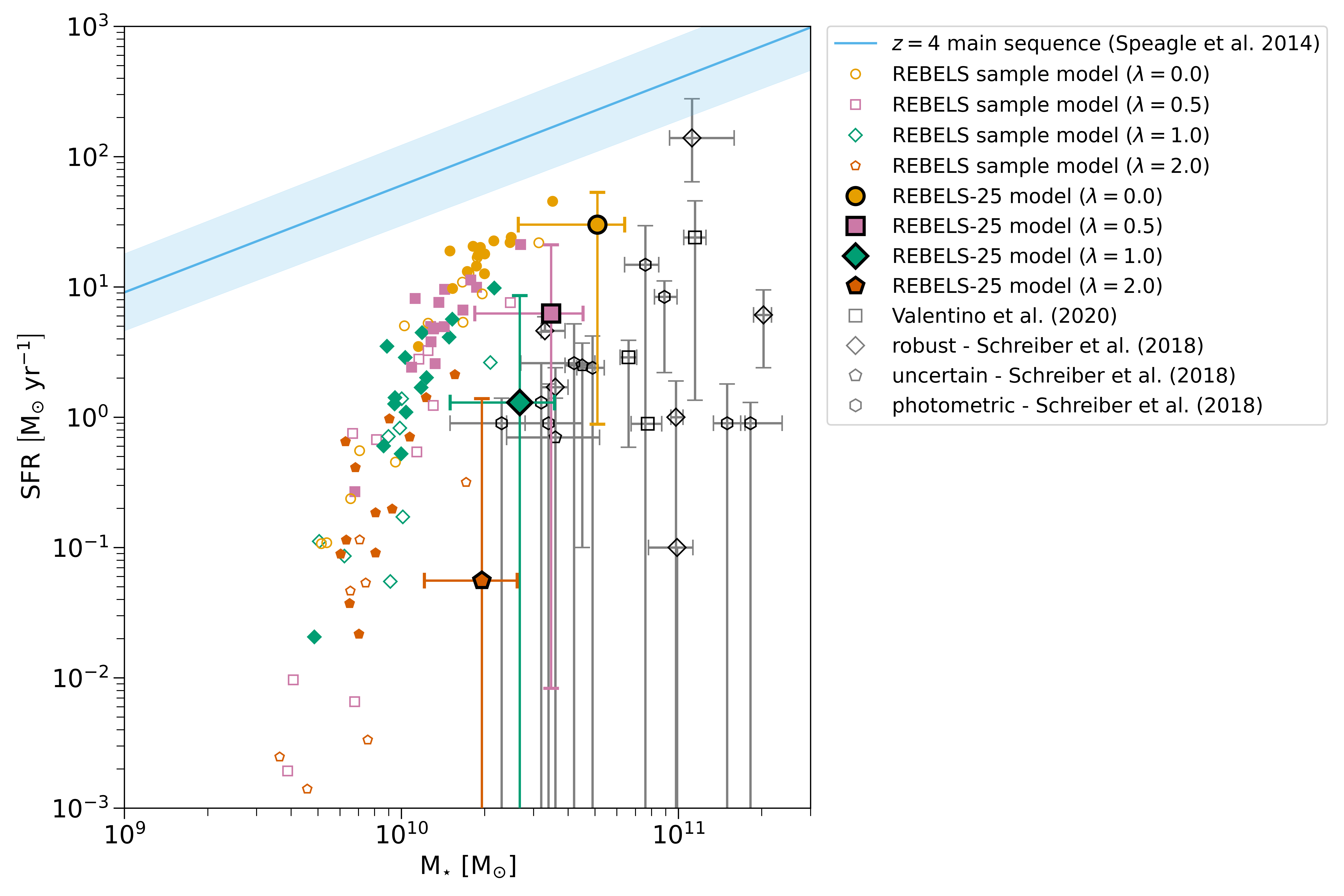
Figure 7: The predicted SFR against the stellar mass for the REBELS sample at $z=4$ derived from a simple conservative model under the assumption of continuous star formation with constant star formation efficiency and no inflow of gas. The REBELS galaxies are shown with filled markers where a continuum flux is reported by (Inami et al., 2022) or with open markers where only an upper limit on the continuum flux (and thus only an upper limit on the obscured star formation) is reported. The different marker shape-colour combinations indicate the mass loading factor of the outflow model, either 0, which is equivalent to no outflow (yellow circles); 0.5 (pink squares); 1 (teal diamonds) or 2 (red pentagons). REBELS-25 is displayed with an additional solid black outline around the marker and with 1 $\sigma$ errorbars. The SFRs and stellar masses of quiescent galaxies observed at $z\sim 4$ are indicated on the plot as open squares (Valentino et al., 2020), open diamonds (the robust spectroscopic sample of Schreiber et al., 2018b), open pentagons (the uncertain spectroscopic sample of Schreiber et al., 2018b) and open hexagons (the photometric sample of Schreiber et al., 2018b). The solid blue line shows the $z=4$ main sequence of Speagle et al. (2014) and the blue shaded area shows its associated 1-$\sigma$ error region.

We consider a simple evolutionary model that includes a declining SFR and the possibility of an outflow. Although inflows are thought to be important at the high redshifts of the EoR (see e.g Sánchez Almeida et al., 2014), the assumption of no inflow, means that this model provides a conservative estimate of the stellar mass evolution of REBELS-25. An inflow would serve to increase the available gas mass for star formation, which would have the effect of increasing the SFR of the galaxy at a given redshift and thus its given stellar mass. Indeed observations of high-z quiescent galaxies (Forrest et al., 2020a) and simulations (Pallottini et al., 2017; Pallottini et al., 2022) suggest that these galaxies may have an SFH consistent with a sustained period of high SFR followed by late quenching. However, restricting ourselves to a conservative lower estimate of the stellar mass allows us to explore the possibility that REBELS-25 is a plausible progenitor of high-z quiescent galaxies.

We model the evolution of the galaxy forward in time, $t$, starting from its currently observed properties at t=0 (corresponding to its observed redshift at $z=7.31$). In this model, we assume an exponentially declining SFR, with fixed star formation efficiency, $\varepsilon$, set by the observed SFR and molecular gas mass at $t=0$, i.e.

$$\varepsilon=\dot{M_{*}}(0)/M_{{\rm H}_{2}}(0).$$ (12)

where $\dot{M_{*}}(0)=\mbox{$199^{+101}_{-63}$}{}~{}\mbox{M${}_{\odot}$}\mbox{${\rm yr}$}^{-1}$ is our measurement of the star formation rate of REBELS-25 and $M_{{\rm H}_{2}}(0)=\mbox{$5.1^{+5.1}_{-2.6}\times 10^{10}$}{}~{}\mbox{M${}_{\odot}$}$ is our measurement of the molecular gas mass. For the outflow, we adopt a model where the mass outflow $\dot{M}_{\rm out}$ rate at $t$ is proportional to the SFR

$$\dot{M}_{\rm out}(t)=\lambda\dot{M}_{*}(t),$$ (13)

where $\lambda$ is the outflow mass loading factor. We consider four scenarios for the strength of the outflow: $\lambda=0,0.5,1.0$ and $2.0$. We note that $\lambda=0$ represents the case with no outflow. With these assumptions the SFR at $t$, $\dot{M_{*}}(t)$, is given by

$$\dot{M}_{*}(t)=\dot{M}_{*}(0)e^{-\varepsilon\left[\left(1-\rho\right)+\lambda\right]t},$$ (14)

where $\rho=0.4$ is the fraction of gas returned to the interstellar medium via stellar feedback (primarily supernovae and stellar winds).

We randomly sample the uncertainty distribution of the currently observed properties of the galaxy in order to determine the uncertainty on these evolutionary tracks. Specifically we create 10000 sets of initial properties, which are randomly sampled from independent Gaussian uncertainty distributions defined by the measured values of these parameters and their associated uncertainties. To determine the upper and lower uncertainty region for the evolutionary tracks, we calculate the 16th and 84th percentiles of the values of SFR and stellar mass from the evolutionary tracks generated from these randomly sampled starting conditions.

We display the resultant evolutionary tracks of SFR and stellar mass for REBELS-25 in Figure 6 compared against observed high-z quiescent galaxies from the literature. These tracks show that, under the assumptions of our model, REBELS-25 could evolve into a massive, low star-formation rate galaxy with properties consistent with the properties of a number of observed high-z quiescent galaxies. However, REBELS-25 does not have sufficient molecular gas mass currently to evolve into the most massive observed high-z quiescent galaxies. In order to do so REBELS-25 would require additional molecular gas mass such as through inflow or the addition of more stellar mass through mergers. We repeat this analysis for all other the galaxies in the REBELS sample with a spectroscopic redshift (Bouwens et al., 2022, Schouws et al. in prep.). We show the predicted SFR and stellar mass at $z\sim 4$ for these galaxies compared to REBELS-25 and a number of high-z quiescent galaxies from the literature observed at $z\sim 4$ in Figure 7. Compared to the REBELS sample as a whole, REBELS-25 has the largest predicted stellar mass at $z=4$ regardless of the outflow mass loading factor that we adopt.

REBELS-25 is able to reach a mass comparable to the lower end of the mass range of high-z quiescent galaxies identified by Glazebrook et al. (2017), Schreiber et al. (2018a) and Valentino et al. (2020), under the conditions of our model. However, the question arises as to how much gas inflow would be required for REBELS-25 to reach a mass similar to the more massive high-z quiescent galaxies that have been detected. We therefore return to consider inflows that we have so far not included in our model, by adding a simple constant inflow term. We compare the results of this model to the masses of the high-redshift quiescent galaxies identified by Glazebrook et al. (2017), Schreiber et al. (2018a) and Valentino et al. (2020) with $z\geq 3.3$. In order for REBELS-25 to reach the median stellar mass of these galaxies at $z\sim 4$, a constant inflow rate of $\sim 25~{}\mbox{M${}_{\odot}$}\mbox{${\rm yr}$}^{-1}$ would be required, and to reach the maximum stellar mass a constant inflow of $\sim 1000~{}\mbox{M${}_{\odot}$}\mbox{${\rm yr}$}^{-1}$ would be required.

5 Conclusions

We have presented ALMA [Cii] and dust continuum observations, obtained as part of the REBELS survey (Bouwens et al., 2022), of REBELS-25. REBELS-25 is a dusty ULIRG, with $L_{\rm IR}$ = $1.5^{+0.8}_{-0.5}\times 10^{12}$ L_⊙, as determined from a monochromatic $\sim 158$ µm flux of $260\pm 22$ µJy (Inami et al., 2022). It has been confirmed at a spectroscopic redshift of 7.31. It has a significant stellar mass ($M_{*}$ = $8^{+4}_{-2}\times 10^{9}$; Bouwens et al. 2022, Stefanon et al. in prep.). In this paper we have used these ALMA observations in conjunction with HST observations of the UV to characterise REBELS-25. Our main conclusions are as follows:

• We determine a [Cii] luminosity of $L_{\mbox{[C{\sc ii}]}{}}=\mbox{$1.7\pm 0.2\times 10^{9}$}$, for the main double-peaked [Cii] emission component of REBELS-25.

• We use our measurement of $L_{\mbox{[C{\sc ii}]}{}}~{}\mbox{L${}_{\odot}$}{}$ to infer a significant molecular gas reservoir of $5.1^{+5.1}_{-2.6}\times 10^{10}$ M_⊙. Combined with our SFR measurement, this gives a short depletion time of $t_{\rm depl,{\rm H}_{2}}=\mbox{$0.3^{+0.3}_{-0.2}$}{}$ Gyr, about half of the predicted main-sequence value.

• We determine a UV + IR star formation rate of $199^{+101}_{-63}$ M_⊙ $\mbox{${\rm yr}$}^{-1}$, which places REBELS-25 a factor of four above an extrapolated Speagle et al. (2014) star formation main-sequence with our adopted stellar mass, which would classify it as starbursting galaxy. However, adopting the non-parametric stellar mass presented by Topping et al. (2022) or the main-sequence derived from the REBELS sample also presented by Topping et al. (2022) would result in its classification as a main-sequence galaxy. In contrast, adopting the $z\sim 5.5$ main sequence presented by Khusanova et al. (2021) would lead to an even stronger classification of the galaxy as a starburst galaxy.

• The majority of the star formation in REBELS-25 is obscured star formation traced by IR emission ($185^{+101}_{-63}$ M_⊙ $\mbox{${\rm yr}$}^{-1}$) and there is a small contribution from unobscured star formation as traced by UV ($14\pm 3$ M_⊙ $\mbox{${\rm yr}$}^{-1}$).

• We find that REBELS-25 exhibits a kinematic profile that appears consistent with a rotating disc. However, due to the large beam of our current [Cii] data, this could equally be the result of merging galaxies whose kinematics are smeared by the beam.

• We find, consistent with an earlier study by Schouws et al. (2022a), that the dust continuum emission is offset from the UV clumps identified by Stefanon et al. (2019). As with similar offsets in lower-redshift dusty star forming galaxies, this can be interpreted as resulting from UV clumps embedded in a disc and visible in areas of low-extinction or as resulting from a disturbed morphology due to a merger.

• We observe an additional [Cii] emission component that may indicate a minor merger or the presence of an outflow. Modelling this emission as coming from a merging galaxy, we measure a molecular gas mass of $9^{+9}_{-5}\times 10^{9}$  M_⊙ (about 18 per cent of REBELS-25’s molecular gas reservoir). If we instead model the emission as coming from an outflow, we estimate a projected (deprojected) atomic mass outflow rate of $\gtrsim 120$ M_⊙ $\mbox{${\rm yr}$}^{-1}$ ($\gtrsim\mbox{$200$}{}$ M_⊙ $\mbox{${\rm yr}$}^{-1}$), corresponding to atomic outflow mass loading factors of $\gtrsim 0.6$ ( $\gtrsim 1.0$). However, due to the difficulty of determining the size of the outflow these numbers are quite uncertain.

• We also investigated the potential evolution of REBELS-25 by considering a simple, conservative evolutionary model with a star formation rate set by a constant star formation efficiency, no inflow of gas and the possibility of constant mass-loading factor outflows. From this model, we find that REBELS-25 could potentially evolve into a galaxy with properties consistent with the population of high-z quiescent galaxies observed at $z\sim 4$ (see e.g Schreiber et al., 2018b; Valentino et al., 2020) without needing to acquire more molecular gas.

In summary, we find that REBELS-25 has significant existing stellar mass, which coupled with a large molecular gas reservoir and significant star formation rate make it a realistic progenitor of high redshift quiescent galaxies. In addition, it has the signatures of complex morphology including potential disc rotation and the possibility of merger and/or outflow activity that requires further high-resolution follow-up to confirm.

Data Availability

The ALMA observations used in this article are available in the ALMA archive https://almascience.eso.org/aq/ and can be accessed with their project codes: 2019.1.01634.L and 2017.1.01217.S. The COSMOS-DASH HST image used available from the Mikulski Archive for Space Telescopes on the COSMOS-DASH page: https://archive.stsci.edu/hlsp/cosmos-dash. The Gaia DR3 data underlying this paper is available from the GAIA archive https://gea.esac.esa.int/archive/. The data underlying this article will be shared on reasonable request to the corresponding author.

Appendix A Models fitted to the spectrum

In Section 3.1, we fit models to the spectrum of REBELS-25 (see Figure 2), which are made up of a linear sum of up to three Gaussian functions of the form

$$c\exp\left(\frac{-(x-\mu)^{2}}{2\sigma^{2}}\right).$$ (15)

The models have either one or two Gaussians to fit the main [Cii] component and either one or no Gaussians to fit the secondary [Cii] component. The model of the secondary [Cii] component is either a broad Gaussian to represent an outflow or a narrow Gaussian to represent a merging galaxy. We also impose constraints on the parameters of our fits. For the Gaussian(s) representing the main component we require $c>0$ mJy and $-350\mbox{${\rm km~{}s^{-1}}$}{}<\mu<250\mbox{${\rm km~{}s^{-1}}$}{}$ . For the Gaussian representing a merger, we require $c>0$ mJy and $250\mbox{${\rm km~{}s^{-1}}$}{}<\mu<750\mbox{${\rm km~{}s^{-1}}$}{}$. Lastly, for the Gaussian representing an outflow we require $c>0$ mJy, $-350\mbox{${\rm km~{}s^{-1}}$}{}<\mu<750\mbox{${\rm km~{}s^{-1}}$}{}$ and $\sigma>150$ ${\rm km~{}s^{-1}}$ . The best-fitting parameters and the reduced $\chi^{2}$ values of the models that we fit are displayed in Table 2.

Table 2: A summary of the models fitted to the spectrum in Section 3.1. The models are a linear sum of between one and three Gaussians of the form in Equation 15.

Model Name	$\chi^{2}_{\rm red}$	$c_{1}$	$\mu_{1}$	$\sigma_{1}$	$c_{2}$	$\mu_{2}$	$\sigma_{2}$	$c_{3}$	$\mu_{3}$	$\sigma_{3}$
		$\mathrm{mJy}$	$\mathrm{km\,s^{-1}}$	$\mathrm{km\,s^{-1}}$	$\mathrm{mJy}$	$\mathrm{km\,s^{-1}}$	$\mathrm{km\,s^{-1}}$	$\mathrm{mJy}$	$\mathrm{km\,s^{-1}}$	$\mathrm{km\,s^{-1}}$
Double Gaussian + merger	1.51	$4.2\pm 0.2$	$-43\pm 10$	$91\pm 9$	$2.8\pm 0.4$	$134\pm 9$	$51\pm 8$	$0.9\pm 0.2$	$514\pm 22$	$102\pm 22$
Double Gaussian + outflow	1.64	$3.8\pm 0.3$	$-45\pm 9$	$77\pm 9$	$2.6\pm 0.3$	$124\pm 9$	$48\pm 8$	$0.6\pm 0.2$	$97\pm 79$	$378\pm 90$
Single Gaussian + merger	1.72	$4.2\pm 0.2$	$4\pm 6$	$133\pm 6$	$0.9\pm 0.2$	$531\pm 21$	$90\pm 22$
Single Gaussian + outflow	1.92	$3.7\pm 0.3$	$-2\pm 8$	$119\pm 11$	$0.5\pm 0.3$	$172\pm 131$	$342\pm 96$
Double Gaussian	1.95	$3.7\pm 0.3$	$20\pm 11$	$137\pm 8$	$1.3\pm 0.4$	$-71\pm 12$	$37\pm 15$
Single Gaussian	2.02	$4.2\pm 0.2$	$5\pm 6$	$134\pm 6$

Appendix B Significance of the secondary [Cii] emission component

We identify both a bright (double-peaked) main [Cii] component and a fainter secondary [Cii] component. In order to investigate the significance of the secondary [Cii] component, we split the data in half and reimage it. The first half of the data was observed on the 22nd of November 2019 and the second half of the data was observed on the 25th of November and the 1st of December 2019. The resulting spectra can be seen in Figure 8 in comparison to the spectrum produced from all of the data combined. We then collapse the datacubes over the line to create a moment-0 map and measure the peak signal to noise in the image plane for the secondary component. With both haves of the data together, we measure a peak signal-to-noise ratio of $4.7$. We see by inspecting the two half-data spectra that the secondary [Cii] component remains visible in both halves of the data. We determine a peak signal-to-noise ratio of 4.0 and 3.1 for the secondary component in first and second halves of the data. We thus conclude that the secondary component is significant.

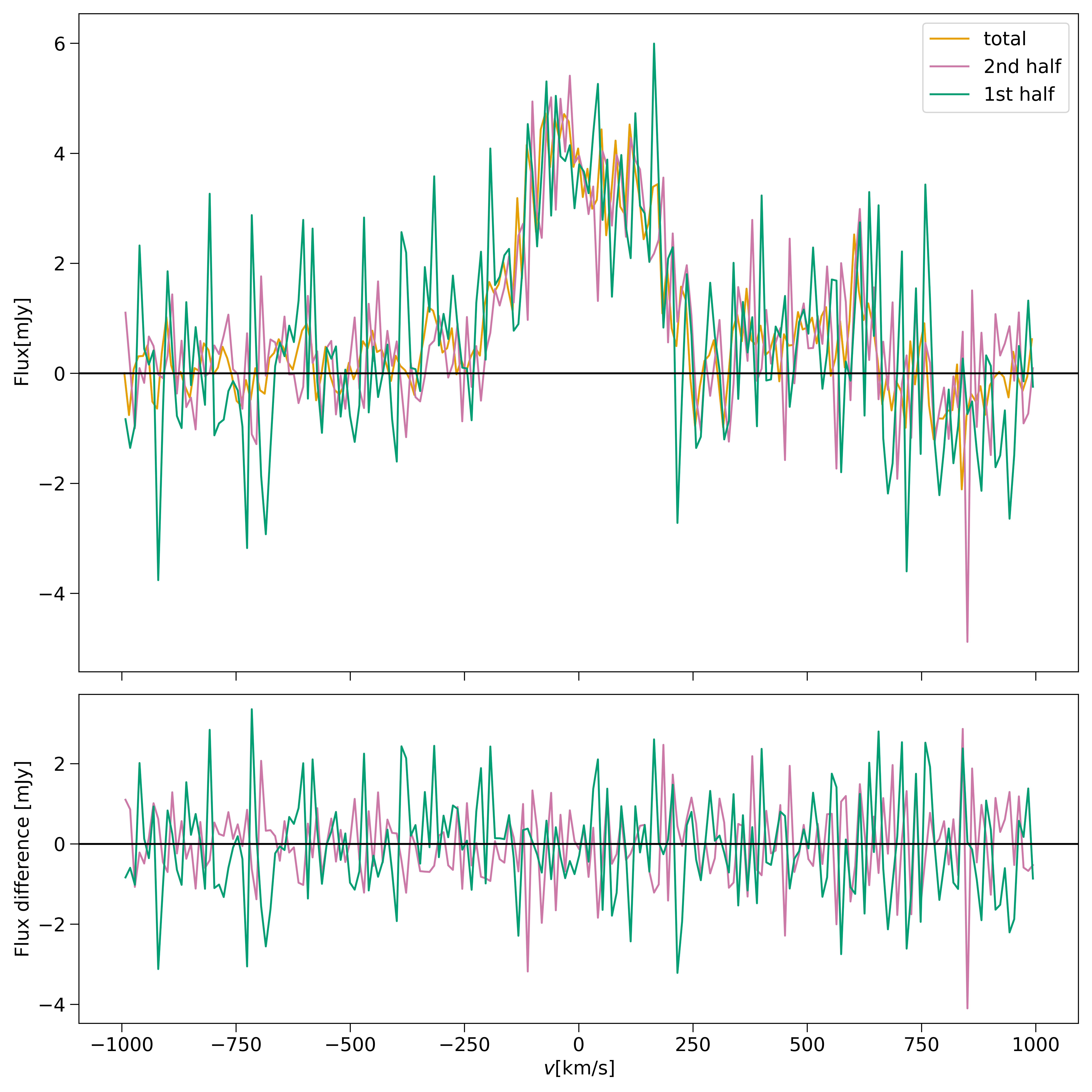
Figure 8: [Top panel] the spectra extracted from data cubes created with all the ALMA data (yellow line), the first half of the ALMA data (pink line) and the second half of the ALMA data (teal line).[ Bottom panel] the flux difference between the two half-data spectra and the total spectrum. Both the main and secondary [Cii] components remain visible in both of the half-data spectra.

¹ Leiden Observatory, Leiden University, P.O. Box 9513, 2300 RA Leiden, The Netherlands
² International Centre for Radio Astronomy Research, University of Western Australia, 35 Stirling Hwy, Crawley, 26WA 6009, Australia
³ ARC Centre of Excellence for All Sky Astrophysics in 3 Dimensions (ASTRO 3D), 2601, Australia
⁴ Faculty of Electrical Engineering, Mathematics and Computer Science, Delft University of Technology, Delft, The Netherlands
⁵ Hiroshima Astrophysical Science Center, Hiroshima University, 1-3-1 Kagamiyama, Higashi-Hiroshima, Hiroshima 739-8526, Japan
⁶ Departament d’Astronomia i Astrofísica, Universitat de València, C. Dr. Moliner 50, E-46100 Burjassot, València, Spain
⁷ Dipartimento di Fisica, Sapienza, Università di Roma, Piazzale Aldo Moro 5, I-00185 Roma, Italy
⁸ INAF/Osservatorio Astrofisico di Arcetri, Largo E. Fermi 5, I-50125 Firenze, Italy
⁹ Sapienza School for Advanced Studies, Viale Regina Elena 291, I-00161 Roma Italy
¹⁰ INAF/Osservatorio Astronomico di Roma, via Frascati 33, I-00078 Monte Porzio Catone, Roma, Italy
¹¹ Istituto Nazionale di Fisica Nucleare, Sezione di Roma1, Piazzale Aldo Moro 2, I-00185 Roma Italy
¹² Kapteyn Astronomical Institute, University of Groningen, NL-9700 AV Groningen, the Netherlands
¹³ Astrophysics Research Institute, Liverpool John Moores University, 146 Brownlow Hill, Liverpool L3 5RF, UK
¹⁴ Jodrell Bank Centre for Astrophysics, Department of Physics and Astronomy, School of Natural Sciences, The University of Manchester,Manchester, M13 9PL, UK
¹⁵ Steward Observatory, University of Arizona, 933 N Cherry Ave, Tucson, AZ 85721, USA
¹⁶ Departmento de Astronomia, Universidad de Chile, Casilla 36-D, Santiago 7591245, Chile
¹⁷ Centro de Astrofisica y Tecnologias Afines (CATA), Camino del Observatorio 1515, Las Condes, Santiago, 7591245, Chile
¹⁸ Observatoire de Genève, CH-1290 Versoix, Switzerland
¹⁹ Cosmic Dawn Center (DAWN), Niels Bohr Institute, University of Copenhagen, Jagtvej 128, København N, DK-2200, Denmark
²⁰National Astronomical Observatory of Japan, 2-21-1, Osawa, Mitaka, Tokyo, Japan
²¹ Nucleo de Astronomia, Facultad de Ingenieria y Ciencias, Universidad Diego Portales, Av. Ejercito 441, Santiago, Chile
²² Scuola Normale Superiore, Piazza dei Cavalieri 7, I- 50126 Pisa, Italy
²³ Waseda Research Institute for Science and Engineering, Faculty of Science and Engineering, Waseda University, 3-4-1 Okubo, Shinjuku, Tokyo 169-8555, Japan
²⁴ Sterrenkundig Observatorium, Ghent University, Krijgslaan 281-S9, B- 9000 Gent, Belgium
²⁵ Dept. of Physics & Astronomy, University College London, Gower Street, London WC1E 6BT, UK
²⁶ Centre for Astrophysics and Supercomputing, Swinburne University of Technology, PO Box 218, Hawthorn, VIC 3112, Australia
²⁷ I. Physikalisches Institut, Universität zu Köln, Zülpicher Strasse 77, D-50937 Köln, Germany

References

- Algera et al. (2023a) Algera H., et al., 2023a, Cold Dust and Low [OIII]/[CII] Ratios: An Evolved Star-forming Population at Redshift 7, doi:10.48550/arXiv.2301.09659
- Algera et al. (2023b) Algera H. S. B., et al., 2023b, MNRAS, 518, 6142
- Astropy Collaboration et al. (2013) Astropy Collaboration et al., 2013, A&A, 558, A33
- Astropy Collaboration et al. (2018) Astropy Collaboration et al., 2018, AJ, 156, 123
- Astropy Collaboration et al. (2022) Astropy Collaboration et al., 2022, ApJ, 935, 167
- Bakx et al. (2020) Bakx T. J. L. C., et al., 2020, MNRAS, 493, 4294
- Bakx et al. (2021) Bakx T. J. L. C., et al., 2021, MNRAS, 508, L58
- Bañados et al. (2019) Bañados E., et al., 2019, ApJ, 881, L23
- Béthermin et al. (2020) Béthermin M., et al., 2020, A&A, 643, A2
- Bigiel et al. (2008) Bigiel F., Leroy A., Walter F., Brinks E., de Blok W. J. G., Madore B., Thornley M. D., 2008, AJ, 136, 2846
- Bigiel et al. (2011) Bigiel F., et al., 2011, ApJL, 730, L13
- Bischetti et al. (2019) Bischetti M., Maiolino R., Carniani S., Fiore F., Piconcelli E., Fluetsch A., 2019, A&A, 630, A59
- Bouwens et al. (2022) Bouwens R. J., et al., 2022, ApJ, 931, 160
- Bowler et al. (2020) Bowler R. A. A., Jarvis M. J., Dunlop J. S., McLure R. J., McLeod D. J., Adams N. J., Milvang-Jensen B., McCracken H. J., 2020, MNRAS, 493, 2059
- Bowler et al. (2022) Bowler R. A. A., Cullen F., McLure R. J., Dunlop J. S., Avison A., 2022, MNRAS, 510, 5088
- Bradley et al. (2022) Bradley L., et al., 2022, Zenodo
- Brammer et al. (2008) Brammer G. B., van Dokkum P. G., Coppi P., 2008, ApJ, 686, 1503
- Bruzual & Charlot (2003) Bruzual G., Charlot S., 2003, MNRAS, 344, 1000
- Calistro Rivera et al. (2018) Calistro Rivera G., et al., 2018, ApJ, 863, 56
- Carnall et al. (2020) Carnall A. C., et al., 2020, MNRAS, 496, 695
- Carniani et al. (2018) Carniani S., et al., 2018, MNRAS, 478, 1170
- Cassata et al. (2020) Cassata P., et al., 2020, A&A, 643, A6
- Cecchi et al. (2019) Cecchi R., Bolzonella M., Cimatti A., Girelli G., 2019, ApJ, 880, L14
- Chabrier (2003) Chabrier G., 2003, PASP, 115, 763
- Chen et al. (2017) Chen C.-C., et al., 2017, ApJ, 846, 108
- Chevallard & Charlot (2016) Chevallard J., Charlot S., 2016, MNRAS, 462, 1415
- Cicone et al. (2014) Cicone C., et al., 2014, A&A, 562, A21
- Cicone et al. (2015) Cicone C., et al., 2015, A&A, 574, A14
- Clements et al. (2018) Clements D. L., et al., 2018, MNRAS, 475, 2097
- Cochrane et al. (2021) Cochrane R. K., et al., 2021, MNRAS, 503, 2622
- Cortes et al. (2022) Cortes P. C., et al., 2022, ALMA Technical Handbook, ALMA Doc. 9.3, ver. 1.0 ISBN 978-3-923524-66-2
- Croxall et al. (2017) Croxall K. V., et al., 2017, ApJ, 845, 96
- Dayal & Ferrara (2018) Dayal P., Ferrara A., 2018, Phys. Rep., 780–782, 1
- Dayal et al. (2014) Dayal P., Ferrara A., Dunlop J. S., Pacucci F., 2014, MNRAS, 445, 2545
- Dayal et al. (2022) Dayal P., et al., 2022, MNRAS, 512, 989
- De Looze et al. (2014) De Looze I., et al., 2014, A&A, 568, A62
- De Vis et al. (2019) De Vis P., et al., 2019, A&A, 623, A5
- Decarli et al. (2018) Decarli R., et al., 2018, ApJ, 854, 97
- Dessauges-Zavadsky et al. (2020) Dessauges-Zavadsky M., et al., 2020, A&A, 643, A5
- Dunlop et al. (2017) Dunlop J. S., et al., 2017, MNRAS, 466, 861
- Eggen et al. (1962) Eggen O. J., Lynden-Bell D., Sandage A. R., 1962, ApJ, 136, 748
- Elbaz et al. (2018) Elbaz D., et al., 2018, A&A, 616, A110
- Fabricius et al. (2021) Fabricius C., et al., 2021, A&A, 649, A5
- Faisst et al. (2020) Faisst A. L., et al., 2020, ApJS, 247, 61
- Fall & Efstathiou (1980) Fall S. M., Efstathiou G., 1980, MNRAS, 193, 189
- Ferrara et al. (2022) Ferrara A., et al., 2022, MNRAS, 512, 58
- Fluetsch et al. (2019) Fluetsch A., et al., 2019, MNRAS, 483, 4586
- Forrest et al. (2020a) Forrest B., et al., 2020a, ApJ, 890, L1
- Forrest et al. (2020b) Forrest B., et al., 2020b, ApJ, 903, 47
- Fudamoto et al. (2021) Fudamoto Y., et al., 2021, Nature, 597, 489
- Fujimoto et al. (2019) Fujimoto S., et al., 2019, ApJ, 887, 107
- Fujimoto et al. (2020) Fujimoto S., et al., 2020, ApJ, 900, 1
- Gaia Collaboration et al. (2016) Gaia Collaboration et al., 2016, A&A, 595, A1
- Gaia Collaboration et al. (2022a) Gaia Collaboration et al., 2022a, Gaia Data Release 3: Summary of the Content and Survey Properties, doi:10.48550/arXiv.2208.00211
- Gaia Collaboration et al. (2022b) Gaia Collaboration et al., 2022b, A&A, 667, A148
- Gallerani et al. (2018) Gallerani S., Pallottini A., Feruglio C., Ferrara A., Maiolino R., Vallini L., Riechers D. A., Pavesi R., 2018, MNRAS, 473, 1909
- Galliano et al. (2018) Galliano F., Galametz M., Jones A. P., 2018, ARA&A, 56, 673
- Ginolfi et al. (2020a) Ginolfi M., et al., 2020a, A&A, 633, A90
- Ginolfi et al. (2020b) Ginolfi M., et al., 2020b, A&A, 643, A7
- Ginsburg et al. (2019) Ginsburg A., et al., 2019, Zenodo
- Girelli et al. (2019) Girelli G., Bolzonella M., Cimatti A., 2019, A&A, 632, A80
- Glazebrook et al. (2017) Glazebrook K., et al., 2017, Nature, 544, 71
- Gruppioni et al. (2020) Gruppioni C., et al., 2020, A&A, 643, A8
- Gutkin et al. (2016) Gutkin J., Charlot S., Bruzual G., 2016, MNRAS, 462, 1757
- Harris et al. (2020) Harris C. R., et al., 2020, Nature, 585, 357