Frequency Enhanced Hybrid Attention Network for Sequential Recommendation

Abstract.

The self-attention mechanism, which equips with a strong capability of modeling long-range dependencies, is one of the extensively used techniques in the sequential recommendation field. However, many recent studies represent that current self-attention based models are low-pass filters and are inadequate to capture high-frequency information. Furthermore, since the items in the user behaviors are intertwined with each other, these models are incomplete to distinguish the inherent periodicity obscured in the time domain. In this work, we shift the perspective to the frequency domain, and propose a novel Frequency Enhanced Hybrid Attention Network for Sequential Recommendation, namely FEARec. In this model, we firstly improve the original time domain self-attention in the frequency domain with a ramp structure to make both low-frequency and high-frequency information could be explicitly learned in our approach. Moreover, we additionally design a similar attention mechanism via auto-correlation in the frequency domain to capture the periodic characteristics and fuse the time and frequency level attention in a union model. Finally, both contrastive learning and frequency regularization are utilized to ensure that multiple views are aligned in both the time domain and frequency domain. Extensive experiments conducted on four widely used benchmark datasets demonstrate that the proposed model performs significantly better than the state-of-the-art approaches.

1. Introduction

In recent years, sequential recommendation (BERT4Rec, ; GRU4Rec, ) has attracted increasing attention from both industry and academic communities. Essentially, the key advantage of sequential recommender models lies in the explicit modeling of item chronological correlations. To capture users’ dynamic sequential information more accurately, recent years have witnessed lots of efforts based on either Markov chains (Markov, ) or Recurrent Neural Networks (RNNs) (GRU4Rec, ). Meanwhile, Transformer (Attention, ) has emerged as a powerful architecture and a dominant force in various research fields and outperformed RNN-based models in the recommendation tasks. Attributed to its strong capability of modeling long-range dependencies in data, various sequential recommender models (SASRec, ; CoSeRec, ; DuoRec, ; BERT4Rec, ; CL4SRec, ; lspp, ; FDSA, ; MMInfoRec, ; ICLRec, ) adopt Transformers as the sequence encoder to capture item correlations via assigning attention weights to items at different positions and obtain high-quality sequence representations.

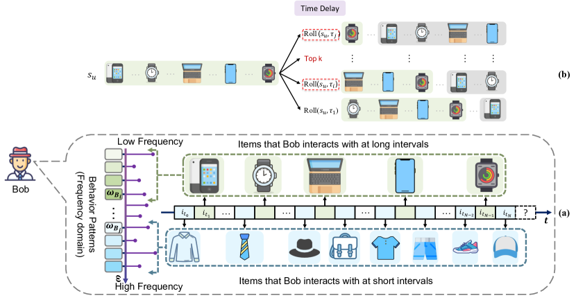
Figure 1. Illustration of our motivations. (a) By shifting the sequential behaviors from the time domain to the frequency domain, the historical item sequence of each user decomposed into multiple behavioral patterns with different frequencies and periods along the $\omega$-axis. (b) By constructing $s_{u}$’s $\tau$ lag sequences $\operatorname{Roll}(s_{u},\tau)$, the periodic pattern can be distinguished from the most similar sequences with the help of discrete Fourier transform.

Despite their effectiveness, self-attention used in current Transformer based models is constantly a low-pass filter, which continuously erases high-frequency information according to the theoretical justification in (howVITwork, ; VIT_seelike_CNN, ). That means, SASRec (SASRec, ) and its variants are highly capable of capturing low-frequencies in the sequential data (iFormer, ), which helps capture a global view of user’s interaction data and the overall evolution of user preference. But owing to its non-local operation (LOCKER, ), they are incompetent in learning high-frequencies information, including those items that interact frequently within a short period.

To alleviate these issues, existing methods import local constraints in different ways to complement Transformer-based models. Such as LSAN (LSAN, ) adopts a novel twin-attention paradigm to capture the global and local preference signals via a self-attention branch and a convolution branch module, respectively. LOCKER (LOCKER, ) combines five local encoders with existing global attention heads to enhance short-term user dynamics modeling. However, the above-mentioned models almost process the historical interactions from the perspective of the time domain, but seldom consider tackling this challenge in the frequency domain, where the reduced high-frequency information can be easily obtained. Take Figure 1(a) for an example, from the viewpoint of the time domain, all the items are chronologically ordered and intertwined along the $t$-axis. With a Discrete Fourier Transform (DFT) (FMLP-Rec, ; GFNet, ), the historical item sequence features of each user can be decomposed into multiple behavioral patterns with different frequencies along the $\omega$-axis, and the input time features are then converted to the frequency domain. Eventually, improving the self-attention operation’s capability for capturing high-frequency information in the frequency domain could become a more direct and effective way.

Moreover, users’ behaviors on the Internet tend to show certain periodic trends (merit_11, ; merit_19, ; merit_21, ). Take Figure 1(b) for an example, there is a periodic behavior pattern hidden in Bob’s low-frequency interactive item, $i.e.$, a watch and laptop are brought after buying a mobile phone. When he recently bought a product with similar characteristics again, a laptop may be a good recommendation to him. However, it is difficult to find the periodic behavior patterns hidden in the sequence by directly calculating the overall attention scores of items in the time domain. But in the frequency domain, there emerges some methods (autoformer, ) constructing models to recognize the periodic characterize with the help of the Fourier transform, which inspires us to tackle this challenge from a new perspective for recommendation.

For these reasons, we shift the perspective to the frequency domain and propose a novel Frequency Enhanced Hybrid Attention Network for Sequential Recommendation (FEARec). Firstly, we improve the time domain self-attention with an adaptive frequency ramp structure. After DFT, we select a specific frequency component as the input feature for each time domain self-attention layer. That enables each layer to focus on different frequency ranges (including not only low-frequency but also high-frequency) to address the problem that self-attention only concentrates on low-frequency. Furthermore, to disentangle the temporal sequence and highlight the inherent periodicity of user behaviors, we design a novel auto-correlation based frequency attention, which is an efficient method to discover the period-based dependencies by calculating the autocorrelation in the frequency domain based on the Wiener-Khinchin theorem (wiener, ). Autocorrelation is used to compare a sequence with a time-delayed version of itself. Specifically, given a user’s behavior sequence $s_{u}$ and its $\tau$ lag sequences $\operatorname{Roll}(s_{u},\tau)$ in Figure 1, the sequential-level connection can be constructed by aggregating the top-$k$ relative sequences ($\operatorname{Roll}(s_{u},\tau_{1}),\cdots,\operatorname{Roll}(s_{u},\tau_{k})$) based on the auto-correlation. Then, we combine the time domain self-attention with frequency domain attention in a union hybrid attention framework. With the help of contrastive and frequency domain regularize loss, a multi-task learning method is applied to increase the supervision information and regularize the training process. The main contributions of this paper can be summarized as follows:

• We shift the perspective to the frequency domain and design a frequency ramp structure to improve existing time domain self-attention.

• We propose a novel frequency domain attention based on an auto-correlation mechanism, which discovers similar period-based dependencies by aggregating most relative time delay sequences.

• We unify the frequency ramp structure with vanilla self-attention and frequency domain attention in one framework and design a frequency domain loss to regularize the model training.

• We conduct extensive experiments on four public datasets, and the experimental results imply the superiority of the FEARec compared to state-of-the-art baselines.

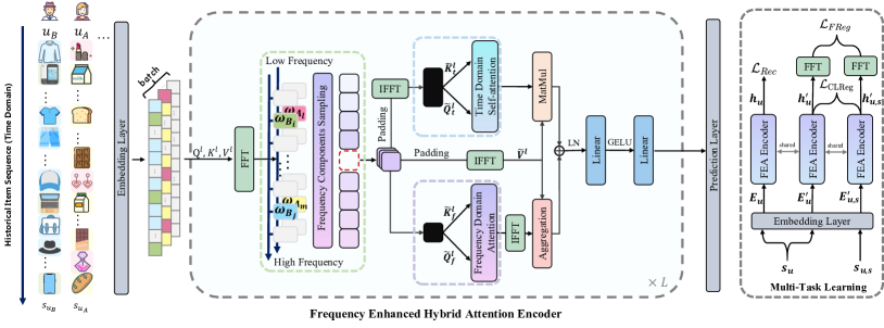
Figure 2. An overview of FEARec. FEARec generates item embedding with positional embedding through the embedding layer, then stacks $L$ hybrid attention blocks to extract user preference in both the item level and frequency level. Supervised contrastive learning and frequency domain regularization are also applied as auxiliary tasks to complement the main task.

2. RELATED WORK

2.1. Sequential Recommendation

Sequential recommendation forecasts future items throughout the user sequence by modeling item transition correlations. Early SR studies are often based on the Markov Chain assumption (Markov, ). Afterward, many deep learning-based sequential recommender models have been developed, e.g., GRU4Rec (GRU4Rec, ), Caser (Caser, ). Later on, self-attention networks have shown great potential in modeling sequence data and a variety of related models are developed, e.g., SASRec (SASRec, ), BERT4Rec (BERT4Rec, ) and S³Rec (S3Rec, ). Recently, many improvements on self-attention based solutions (related28, ; related15, ; related7, ; related5, ; related29, ; related18, ; related3, ; STOSA, ) are proposed to learn better representations of user preference. Most of them use the next-item supervised training style as their training scheme. The other training scheme usually has extra auxiliary training tasks. CL4SRec (CL4SRec, ) applies a contrastive strategy to multiple views generated by data augmentation. CoSeRec (CoSeRec, ) introduces more augmentation operations to train robust sequence representations. DuoRec (DuoRec, ) combines recommendation loss with unsupervised learning and supervised contrastive learning to optimize the SR models. Despite the success of these models in SR, they ignored important information hidden in the frequency domain.

2.2. Frequency Domain Learning

Fourier transform has been an important tool in digital signal processing and graph signal processing for decades (related35, ; related1, ; SIGIR2022, ; graph, ). There are a variety of works that incorporate Fourier transform in computer vision (learninginFD, ; fastfourierconvolution, ; resolution, ; FFC-SE, ; GFNet, ) and natural language processing (NLP1, ; FNET, ). Very recent works try to leverage Fourier transform enhanced model for long-term series forecasting (autoformer, ; FEDformer, ) and partial differential equations solving (FNO, ; AFNO, ; UFNO, ). However, there are few Fourier-related works in the sequential recommendation. More recently, FMLP-Rec (FMLP-Rec, ) first introduce a filter-enhanced MLP for SR, which multiplies a global filter to remove noise in the frequency domain. However, the global filter tends to give greater weight to low frequencies and underrate relatively high frequencies.

3. Proposed Method

In this section, we present the details of the proposed Frequency Enhanced Hybrid Attention Network for Sequential Recommendat- ion namely (FEARec). As shown in Figure 2, after the embedding layer we first transform the embeddings of item sequences from the time domain to the frequency domain by using Fast Fourier Transform (FFT) algorithm mentioned in Appendix A.1.2. Then hybrid attention is conducted on the sampled frequency components, which captures attention scores and periodic behavior patterns of different frequency bands simultaneously. Finally, we apply contrastive learning and frequency domain loss to improve representations in both time and frequency domains

3.1. Embedding Layer

Sequential Recommendation focus on modeling the user behavior sequence of implicit feedback, which is a list of item IDs in SR. In this paper, the item ID set is denoted by $\mathcal{I}=\{i_{1},i_{2},...,i_{|\mathcal{I}|}\}$ and user ID set is represented as $\mathcal{U}=\{u_{1},u_{2},...,u_{|\mathcal{U}|}\}$, where $i\in\mathcal{I}$ denotes an item and $u\in\mathcal{U}$ denotes a user. In this way, the set of user behavior can be represented as $S=\{s_{1},s_{2},...,s_{|\mathcal{U}|}\}$. In SR, the user’s behavior sequence is usually chronologically ordered, $i.e.$, $s_{u}=[i_{1}^{(u)},i_{2}^{(u)},...,i_{t}^{(u)},...,i_{N}^{(u)}]$, where $s_{u}\in S,u\in\mathcal{U}$, and $i_{t}^{(u)}\in\mathcal{I}$ is the item that user $u$ interacts at time step $t$ and $N$ is the sequence length. For $s_{u}$, it is embedded as:

(1) $$\mathbf{E}_{u}=[\mathbf{e}_{1}^{(u)},\mathbf{e}_{2}^{(u)},...,\mathbf{e}_{N}^{(u)}]$$

where $\mathbf{e}_{t}^{(u)}$ is the embedding of item $i_{t}^{(u)}$. To make our model sensitive to the positions of items, we adopt positional embedding to inject additional positional information while maintaining the same embedding dimensions of the item embedding. Moreover, dropout and layer normalization operations are also implemented:

(2) $$\mathbf{E}_{u}=\operatorname{Dropout}(\text{LayerNorm}(\mathbf{E}_{u}+\mathbf{P}))$$

It is worth noting that each item has a unique ID different from each other, but after the embedding layer, similar items may have the same feature value.

3.2. Frequency Enhanced Hybrid Attention Encoder

Based on the embedding layer, we develop the item encoder by stacking $L$ Frequency Enhanced hybrid Attention (FEA) blocks, which generally consists of three modules, $i.e.$, frequency ramp structure, hybrid attention layer, and the point-wise Feed Forward Network (FFN). Since FEARec focuses on capturing specific frequency spectrum at different layers, we first introduce the frequency ramp structure for each layer, and then present other modules for the sampled frequencies at a certain layer.

3.2.1. Frequency Ramp Structure

In FEARec, instead of preserving all frequency components, we only extract a subset of frequencies for each layer to guarantee that different attention blocks focus on different spectrums. This strategy is used in both time domain attention and frequency domain attention as shown in Figure 2.

First, given the input item representation matrix $\mathbf{H}^{l}\in\mathbb{R}^{N\times D}$ of the $l$-th layer and $\mathbf{H}^{0}=\mathbf{E}_{u}$, we could execute FFT denoted as $\mathcal{F}(\cdot)$ along the item dimension to transform the input item representation matrix $\mathbf{H}^{l}$ to the frequency domain:

(3) $$\mathcal{F}(\mathbf{H}^{l})\rightarrow\mathbf{X}^{l}\in\mathbb{C}^{N\times D}$$

As said in Appendix A.1.1, due to the conjugate symmetric property in the frequency domain, only half of the spectrum is used in FEARec

(4) $$M={\lceil N/2\rceil}+1$$

As a result, the sequence length of $\mathbf{X}^{l}$ almost equals half of $\mathbf{H}^{l}$. Note that $\mathbf{X}^{l}$ is a complex tensor and represents the spectrum of $\mathbf{H}^{l}$.

Then, as shown in Figure 3(a), we gradually select a specific frequency range for each layer and formulate this select operator as

(5) $$\tilde{\boldsymbol{X}}^{l}=\operatorname{Sample}_{\alpha}^{l}(\boldsymbol{X}^{l})=\boldsymbol{X}^{l}[p^{l}:q^{l},:]$$

where $\tilde{\boldsymbol{X}}^{l}\in\mathbb{C}^{F\times D}$ and $F\in\mathbb{N}$ denotes the length of sampled frequency features. We set $\alpha=\frac{F}{M}$ as the initial sampling ratio and all frequency components are retained when $\alpha$ =1. The indexes of the sampled frequency components ($p^{l}$ and $q^{l}$) are determined by the position of the current layer in the model. Taking into account that top layers focus more on modeling low-frequency global information while bottom layers are more capable of capturing high-frequency details (iFormer, ), we choose the direction from high frequency to low frequency. For example, for $l$-th layer:

(6) $$p^{l}=M(1-\alpha)(1-\frac{l-1}{L-1})$$

(7) $$q^{l}=p^{l}+\alpha M$$

From Figure 3(b), when $\alpha>\frac{1}{L}$, the frequencies of different layers are overlapped. To avoid the problem of missing frequencies when $\alpha\leq\frac{1}{L}$, we adopt average sampling to ensure that all frequencies are retained:

(8) $$p^{l}=M(1-\frac{l}{L})$$

(9) $$q^{l}=p^{l}+\frac{M}{L}$$

In this way, the whole spectrum is split into several frequency components and preprocessed in different layers. That convenient for us to capture different frequency patterns, and explicitly model high-frequency information that is overlooked by classical self-attention operation.

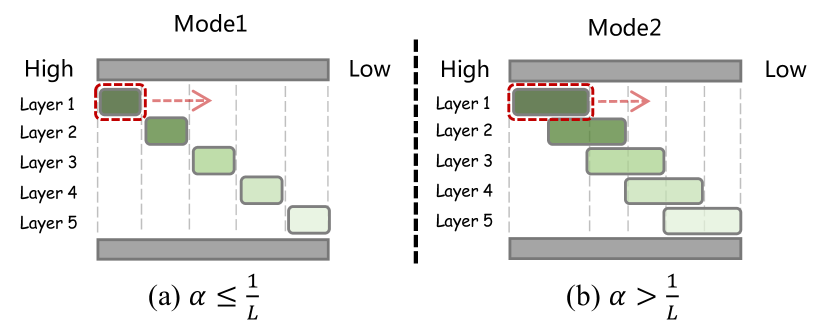
Figure 3. Frequency ramp sampling. When $\alpha\leq\frac{1}{L}$ sampling mode1 is adopted, and $\alpha>\frac{1}{L}$ sampling mode2 is adopted.

3.2.2. Time Domain Self-Attention Layer

As shown in Figure 3, we propose the time domain self-attention to expand the information utilization. For the embedding $\mathbf{H}^{l}$, after linear projector, we get the queries $\boldsymbol{Q}^{l}\in\mathbb{R}^{N\times D}$, keys $\boldsymbol{K}^{l}\in\mathbb{R}^{N\times D}$, and values $\boldsymbol{V}^{l}\in\mathbb{R}^{N\times D}$. Then we convert $\boldsymbol{Q}^{l}$, $\boldsymbol{K}^{l}$, $\boldsymbol{V}^{l}$ to frequency by FFT and sample a Specific frequency components for each layer. Note that, before computing the attention weights in the time domain, the sampled frequencies need to be zero-padded from $\mathbb{C}^{\alpha M\times D}$ to $\mathbb{C}^{M\times D}$. The whole process is represented as:

(10) $$\tilde{\boldsymbol{Q}}^{l}_{t} =\mathcal{F}^{-1}(\operatorname{Padding}(\operatorname{Sample}^{l}_{\alpha}(\mathcal{F}(\boldsymbol{Q}^{l}))))$$

$$\tilde{\boldsymbol{K}}^{l}_{t} =\mathcal{F}^{-1}(\operatorname{Padding}(\operatorname{Sample}^{l}_{\alpha}(\mathcal{F}(\boldsymbol{K}^{l}))))$$

$$\tilde{\boldsymbol{V}}^{l} =\mathcal{F}^{-1}(\operatorname{Padding}(\operatorname{Sample}^{l}_{\alpha}(\mathcal{F}(\boldsymbol{V}^{l}))))$$

and

(11) $$\operatorname{Attention}(\tilde{\boldsymbol{Q}}^{l}_{t},\tilde{\boldsymbol{K}}^{l}_{t},\tilde{\boldsymbol{V}}^{l})=\operatorname{softmax}(\frac{\tilde{\boldsymbol{Q}}^{l}_{t}(\tilde{\boldsymbol{K}}^{l}_{t})^{\top}}{\sqrt{D}})\tilde{\boldsymbol{V}}^{l}$$

In this way, our time domain self-attention can learn not only the low-frequency information in the top layers but also the high-frequency in the bottom layers, thus boosting the model’s capability of capturing local behaviors. For the multi-head version used in FEARec, given hidden variables of $D$ channels, $h$ heads, the query, key and value for $i$-th head $\mathcal{Q}_{i}$, $\mathcal{K}_{i}$, $\mathcal{V}_{i}$ $\in\mathbb{R}^{N\times\frac{D}{h}},i\in\{1,...,h\}$, we have:

(12) $$\operatorname{MultiHead}(\mathcal{Q},\mathcal{K},\mathcal{V}) =\operatorname{Concat}(\text{head}_{1},...,\text{head}_{h})\mathcal{W}$$

$$\text{where head}_{i} =\text{Attention}(\mathcal{Q}_{i},\mathcal{K}_{i},\mathcal{V}_{i})$$

Where learnable output matrix $\mathcal{W\in\mathbb{R}^{D\times D}}$. Hence, the multi-head attention operation for $\tilde{\boldsymbol{Q}}^{l}_{t},\tilde{\boldsymbol{K}}^{l}_{t},\tilde{\boldsymbol{V}}^{l}$ in time domain equals to $\operatorname{MultiHead}_{time}(\tilde{\boldsymbol{Q}}^{l}_{t},\tilde{\boldsymbol{K}}^{l}_{t},\tilde{\boldsymbol{V}}^{l})$.

3.2.3. Frequency Domain Attention Layer

Existing self-attentive sequential recommenders tend to capture a global view of user interactions at the item level, missing the periodic similar behavior patterns captured at the sequence level. As discussed in Section 1, by calculating the auto-correlation, we can find the most related time-delay sequences in the frequency domain and thus discover the periodicity hidden in the behaviors. Specifically, as shown as Figure 1, given a finite sequence of user $s_{u}=[i_{1}^{(u)},i_{2}^{(u)},i_{3}^{(u)},\cdots,i_{N-1}^{(u)},i_{N}^{(u)}]$, the time delay operation is defined as $\operatorname{Roll}(s_{u},\ \tau)$, where $\tau\in\{1,\cdots,N\}$ indicates the time lag and $\operatorname{Roll}(s_{u},\ \tau)$ can be formulated as:

(13) $$\operatorname{Roll}(s_{u},\tau) =[i_{\tau+1}^{(u)},\cdots,i_{N}^{(u)},i_{1}^{(u)},\cdots,i_{\tau}^{(u)}]$$

where $\operatorname{Roll}(s_{u},\ N)=s_{u}$. Its corresponding embedding matrix is denoted as $\tilde{\boldsymbol{V}}_{\tau}^{l}$. We perform a similar attention mechanism via auto-correlation in the frequency domain. For the queries $\boldsymbol{Q}^{l}\in\mathbb{R}^{N\times D}$, keys $\boldsymbol{K}^{l}\in\mathbb{R}^{N\times D}$, and values $\boldsymbol{V}^{l}\in\mathbb{R}^{N\times D}$, the auto-correlation is defined as

(14) $$\tilde{\boldsymbol{Q}}^{l}_{f} =\operatorname{Sample}^{l}_{\alpha}(\mathcal{F}(\boldsymbol{Q}^{l}))$$

$$\tilde{\boldsymbol{K}}^{l}_{f} =\operatorname{Sample}^{l}_{\alpha}(\mathcal{F}(\boldsymbol{K}^{l}))$$

$$\mathcal{R}_{\tilde{\boldsymbol{Q}}^{l}_{f},\tilde{\boldsymbol{K}}^{l}_{f}}(\tau) =\mathcal{F}^{-1}(\operatorname{Padding}(\tilde{\boldsymbol{Q}}^{l}_{f}\odot(\tilde{\boldsymbol{K}}^{l}_{f})^{*}))$$

where $\odot$ represents the element-wise product and * means the conjugate operation. We denote the sampled feature as $\tilde{\boldsymbol{Q}}^{l}_{f},\tilde{\boldsymbol{K}}^{l}_{f}\in\mathbb{C}^{\alpha M\times D}$. $\tilde{\boldsymbol{Q}}^{l}_{f}\odot(\tilde{\boldsymbol{K}}^{l}_{f})^{*}\in\mathbb{C}^{\alpha M\times D}$ needs to be zero-padded to $\mathbb{C}^{M\times D}$ before performing inverse Fourier transform. Since the information used to compute the attention scores is coming from within the same sequence, here we consider it to be auto-correlation rather than cross-correlation. The auto-correlation $\mathcal{R}_{\tilde{\boldsymbol{Q}}^{l}_{f},\tilde{\boldsymbol{K}}^{l}_{f}}(\tau)\in\mathbb{R}^{N\times D}$ is based on the Wiener-Khinchin theorem (more details in the Appendix A.2). We further conduct $\operatorname{MEAN}$ operation on $\mathcal{R}_{\tilde{\boldsymbol{Q}}^{l}_{f},\tilde{\boldsymbol{K}}^{l}_{f}}(\tau)$ to transfer its dimension $\mathbb{R}^{N\times D}$ into $\mathbb{R}^{N}$.

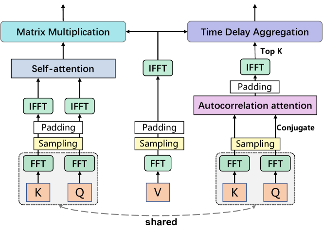
Figure 4. The architecture of hybrid attention layer.

The auto-correlation refers to the correlation of a time sequence with its own past and future, we choose the most related $\tau_{i},...,\tau_{k}$ from $\mathcal{R}_{\tilde{\boldsymbol{Q}}^{l}_{f},\tilde{\boldsymbol{K}}^{l}_{f}}(\tau)$:

(15) $$\tau_{1},\cdots,\tau_{k}=\underset{\tau\in\{1,\cdots,N\}}{\arg\operatorname{Topk}}(\mathcal{R}_{\tilde{\boldsymbol{Q}}^{l}_{f},\tilde{\boldsymbol{K}}^{l}_{f}}(\tau))$$

where $\arg\operatorname{Topk}(\cdot)$ is to get the arguments of the Top $k$ auto-correlation and $k=\lfloor m\times logN\rfloor$. In this way, we get the most relevant time delay sequences $\operatorname{Roll}(s_{u},\tau_{i})$, $\tau_{i}\in\{\tau_{1},\cdots,\tau_{k}\}$. Then, the attention weights of different sequences are calculated as:

(16) $$\widehat{\mathcal{R}}_{\tilde{\boldsymbol{Q}}^{l}_{f},\tilde{\boldsymbol{K}}^{l}_{f}}\left(\tau_{1}\right),\cdots,\widehat{\mathcal{R}}_{\tilde{\boldsymbol{Q}}^{l}_{f},\tilde{\boldsymbol{K}}^{l}_{f}}\left(\tau_{k}\right)=$$

$$\operatorname{SoftMax}(\mathcal{R}_{\tilde{\boldsymbol{Q}}^{l}_{f},\tilde{\boldsymbol{K}}^{l}_{f}}\left(\tau_{1}\right),\cdots,\mathcal{R}_{\tilde{\boldsymbol{Q}}^{l}_{f},\tilde{\boldsymbol{K}}^{l}_{f}}\left(\tau_{k}\right))$$

Hence, the $k$ most similar sequences can be aggregated by multiplying with their corresponding auto-correlations, which is called time delay aggregation in Figure 4:

(17) $$\text{ Auto-Correlation }(\tilde{\boldsymbol{Q}}^{l}_{f},\tilde{\boldsymbol{K}}^{l}_{f},\tilde{\boldsymbol{V}}^{l})=\sum_{i=1}^{k}\tilde{\boldsymbol{V}}_{\tau_{i}}^{l}\widehat{\mathcal{R}}_{\tilde{\boldsymbol{Q}}^{l}_{f},\tilde{\boldsymbol{K}}^{l}_{f}}(\tau_{i})$$

where $\text{Auto-Correlation }(\tilde{\boldsymbol{Q}}^{l}_{f},\tilde{\boldsymbol{K}}^{l}_{f},\tilde{\boldsymbol{V}}^{l})\in\mathbb{R}^{N\times D}$. The multi-head attention operation is also conducted for $\tilde{\boldsymbol{Q}}^{l}_{f},\tilde{\boldsymbol{K}}^{l}_{f},\tilde{\boldsymbol{V}}^{l}$ in frequency domain, which equals to $\operatorname{MultiHead}_{Frequency}(\tilde{\boldsymbol{Q}}^{l}_{f},\tilde{\boldsymbol{K}}^{l}_{f},\tilde{\boldsymbol{V}}^{l})$. Finally, we sum the output of the frequency domain attention module and the output of the time domain attention module with the hyperparameter $\gamma$.

(18) $$\widehat{\mathbf{H}}^{l}= \gamma\operatorname{MultiHead}_{Time}(\tilde{\boldsymbol{Q}}^{l}_{t},\tilde{\boldsymbol{K}}^{l}_{t},\tilde{\boldsymbol{V}}^{l})+$$

$$(1-\gamma)\operatorname{MultiHead}_{Frequency}(\tilde{\boldsymbol{Q}}^{l}_{f},\tilde{\boldsymbol{K}}^{l}_{f},\tilde{\boldsymbol{V}}^{l})$$

3.2.4. Point-wise Feed Forward Network

The frequency domain attention and time domain self-attention are still linear operations, which fail to model complex non-linear relations. To make the network non-linear, we use a two-layer MLP with a GELU activation function. The process is defined as follows:

(19) $$\tilde{\mathbf{H}}^{l}=\operatorname{FFN}(\widehat{\mathbf{H}}^{l})=(\operatorname{GELU}(\widehat{\mathbf{H}}^{l}\mathbf{W}^{l}_{1}+\mathbf{b}^{l}_{1}))\mathbf{W}^{l}_{2}+\mathbf{b}^{l}_{2}$$

where $\mathbf{W}^{l}_{1},\mathbf{W}^{l}_{2}\in\mathbb{R}^{d\times d}$ and $\mathbf{b}^{l}_{1},\mathbf{b}^{l}_{2}\in\mathbb{R}^{1\times d}$ are learnable parameters. To avoid overfitting, $dropout$ layer, residual connection structure, and layer normalization operations are applied on the obtained output $\mathbf{H}^{l+1}$, as shown below:

(20) $$\mathbf{H}^{l+1}=\operatorname{LayerNorm}(\mathbf{H}^{l}+\widehat{\mathbf{H}}^{l}+\operatorname{Dropout}(\tilde{\mathbf{H}}^{l}))$$

3.3. Prediction Layer

After $L$ FEA blocks that hierarchically extract behavior pattern information of previously interacted items, we get the final combined representation of behavior sequences. Based on the preference representation $\mathbf{H}^{L}$, we multiply it by the item embedding matrix $\mathbf{E}\in\mathbb{R}^{|\mathcal{I}|\times D}$ to predict the relevance of the candidate item and use $\operatorname{softmax}$ to convert it into recommendation probability:

(21) $$\mathbf{\hat{y}}=\operatorname{softmax}(\mathbf{E}^{\top}\mathbf{H}^{L})$$

Hence, we expect that the true item $i$ adopted by user $u$ can lead to a higher score $\hat{y_{i}}$. Therefore, we adopt the cross-entropy loss to optimize the model parameter. The objective function of SR can be formulated as:

(22) $$\mathcal{L}_{Rec}=-\sum_{i=1}^{|I|}y_{i}\log\left(\hat{y}_{i}\right)+\left(1-y_{i}\right)\log\left(1-\hat{y}_{i}\right)$$

3.4. Multi-Task Learning

To enhance the training of hybrid attention to capture attention scores and periodic behavior patterns of different frequency bands of user sequence, we leverage a multi-task training strategy to jointly optimize the main recommendation loss with auxiliary dual domain regularization.

3.4.1. Contrastive Learning

Contrastive learning aims to minimize the difference between differently augmented views of the same user and maximize the difference between the augmented sequences derived from different users.

Although previous augmentations methods (CL4SRec, ) including item cropping, masking, and reordering help to enhance the performance of SR models, the data-level augmentations cannot guarantee a high level of semantic similarity (DuoRec, ). Instead of using typical data augmentations, we use a dropout-based augmentations methods as shown in the right part of Figure 2, which is proposed in (R-drop, ; DuoRec, ). We let $\mathbf{E}_{u}$ and $\mathbf{E}_{u}^{\prime}$ pass through the FEA encoder twice for two output views ${\mathbf{H}^{L}_{u}}$ and $({\mathbf{H}^{L}_{u}})^{\prime}$ respectively and model the frequency components to construct harder positive samples by mixing the frequency feature extract from time domain self-attention and frequency autocorrelation attention. Since there are different dropout layers in the embedding layer and hybrid attention module, we will get two different numerical features but similar semantics. Besides, in order to increase the supervision signal of contrast learning, we follow DuoRec (DuoRec, ) and use a sequence $s_{u,s}$ with the same target as $s_{u}$ as the positive sample of supervised contrast learning. All the other augmented samples in the training batch are treated as negative samples in order to efficiently create the negative samples for an augmented pair of samples (represented as $neg$).

For the batch $\mathcal{B}$, the contrastive regularization is defined as:

(23) $$\mathcal{L}_{\mathrm{CLReg}}=\mathcal{L}_{\mathrm{CLReg}}(\mathbf{h}^{\prime}_{u},{\mathbf{h}^{\prime}_{u,s}})+\mathcal{L}_{\mathrm{CLReg}}({\mathbf{h}^{\prime}_{u,s}},\mathbf{h}^{\prime}_{u})$$

(24) $$\mathcal{L}_{\text{CLReg}(\mathbf{h}^{\prime}_{u},{\mathbf{h}^{\prime}_{u,s}})}=-\log\frac{\exp(\operatorname{sim}(\mathbf{h}^{\prime}_{u},{\mathbf{h}^{\prime}_{u,s}}))}{\sum_{neg}\exp(\operatorname{sim}(\mathbf{h}^{\prime}_{u},\mathbf{h}_{neg}))}$$

where $sim(\cdot)$ is dot product and $\mathbf{h}^{\prime}_{u}$ and $\mathbf{h}^{\prime}_{u,s}$ represent unsupervised and supervised augmented views, respectively, defined as follows:

(25) $$\mathbf{h}^{\prime}_{u}=(\mathbf{H}^{L}_{u})^{\prime}[-1],\quad{\mathbf{h}^{\prime}_{u,s}}=({\mathbf{H}^{L}_{u,s}})^{\prime}[-1]$$

3.4.2. Frequency Domain Regularization

The contrastive loss is intuitively performing the push and pull game according to Equation 24 in the time domain. Since time-domain and frequency-domain features represent the same semantics, but only in different domains, we assume that the frequency spectrum of similar time-domain features should also be similar. To ensure the alignment of the representation of different augmented views in the frequency domain, we suggest an L1 regularization in the frequency domain as a complement to FEARec, which contributes to enriching the regularization of the spectrum of the augmented views.

(26) $$\mathcal{L}_{FReg} =\|\mathcal{F}(\mathbf{h}_{u}^{\prime})-\mathcal{F}(\mathbf{h}^{\prime}_{u,s})\|_{1}$$

3.4.3. Train and Inference

Thus, the overall objective of FEARec with $\lambda$ scale weight is:

(27) $$\ell=\ell_{\mathrm{Rec}}+\lambda_{1}\ell_{\mathrm{CReg}}+\lambda_{2}\ell_{\mathrm{FReg}}$$

where $\lambda$ is the hyperparameter to control the strengths of contrastive regularization.

4. EXPERIMENT

In this section, we first briefly describe the settings in our experiments and then conduct extensive experiments to evaluate our proposed model by answering the following research questions:

• RQ1: How does FEARec perform compared with state-of-the-art SR models?

• RQ2: How do key components, such as frequency sampling, time domain self-attention and frequency domain attention affect the performance of FEARec respectively?

• RQ3: What is the influence of different hyper-parameters in FEARec?

• RQ4: Do frequency domain attention and time domain attention focus on the same features?

4.1. Experimental Setup

4.1.1. Dataset

We conduct experiments on four publicly available benchmark datasets. Beauty, Clothing, and Sports are three subsets of Amazon Product dataset, which is known for high sparsity and short sequence lengths. MovieLens-1M is a large and dense dataset consisting of long item sequences collected from the movie recommendation site MovieLens. While ML-1M only contains about 1 million interactions. For all datasets, users/items interacted with less than 5 items/users were removed(Timeinterval, ; BERT4Rec, ). The statistics of the four datasets after preprocessing are summarized in Table 1.

4.1.2. Evaluation Metrics

In evaluation, we adopt the leave-one-out strategy for each user’s item sequence. As suggested by (KDD, ), we rank the predictions over the whole item set without negative sampling. We report the widely used Top-$n$ metrics HR@$n$ (Hit Rate) and NDCG@$n$ (Normalized Discounted Cumulative Gain) to evaluate the recommended lists, where $n$ is set to 5, 10.

Table 1. Statistics of the datasets after preprocessing.

Specs. Beauty Clothing Sports ML-1M # Users 22,363 39,387 35,598 6,041 # Items 12,101 23,033 18,357 3,417 # Avg.Length 8.9 7.1 8.3 165.5 # Actions 198,502 278,677 296,337 999,611 Sparsity 99.93% 99.97% 99.95% 95.16%

Table 2. Overall performance over four datasets. Bold scores represent the highest results of all methods. Underlined scores stand for the highest results from previous methods. The FEARec achieves the state-of-the-art result among all baseline models.

Datasets Metric BPR-MF GRU4Rec Caser SASRec BERT4Rec FMLP-Rec CL4SRec CoSeRec DuoRec FEARec Improv. Beauty HR@5 0.0120 0.0164 0.0259 0.0365 0.0193 0.0398 0.0401 0.0537 0.0546 0.0597 9.34% HR@10 0.0299 0.0365 0.0418 0.0627 0.0401 0.0632 0.0683 0.0752 0.0845 0.0884 4.61% NDCG@5 0.0040 0.0086 0.0127 0.0236 0.0187 0.0258 0.0223 0.0361 0.0352 0.0366 3.97% NDCG@10 0.0053 0.0142 0.0253 0.0281 0.0254 0.0333 0.0317 0.0430 0.0443 0.0459 3.61% Clothing HR@5 0.0067 0.0095 0.0108 0.0168 0.0125 0.0173 0.0168 0.0175 0.0193 0.0214 10.88% HR@10 0.0094 0.0165 0.0174 0.0272 0.0208 0.0277 0.0266 0.279 0.0302 0.0323 6.95% NDCG@5 0.0052 0.0061 0.0067 0.0091 0.0075 0.0098 0.0090 0.0095 0.0113 0.0121 7.08% NDCG@10 0.0069 0.0083 0.0098 0.0124 0.0102 0.0127 0.0121 0.0131 0.0148 0.0156 5.41% Sports HR@5 0.0092 0.0137 0.0139 0.0218 0.0176 0.0218 0.0227 0.0287 0.0326 0.0353 8.28% HR@10 0.0188 0.0274 0.0231 0.0336 0.0326 0.0344 0.0374 0.0437 0.0498 0.0547 9.84% NDCG@5 0.0040 0.0096 0.0085 0.0127 0.0105 0.0144 0.0129 0.0196 0.0208 0.0216 3.85% NDCG@10 0.0051 0.0137 0.0126 0.0169 0.0153 0.0185 0.0184 0.0242 0.0262 0.0272 3.82% ML-1M HR@5 0.0078 0.0763 0.0816 0.1087 0.0733 0.1109 0.1147 0.1262 0.2038 0.2212 8.54% HR@10 0.0162 0.1658 0.1593 0.1904 0.1323 0.1932 0.1975 0.2212 0.2946 0.3123 6.01% NDCG@5 0.0052 0.0385 0.0372 0.0638 0.0432 0.0657 0.0662 0.0761 0.1390 0.1523 9.57% NDCG@10 0.0079 0.0671 0.0624 0.0910 0.0619 0.0918 0.0928 0.1021 0.1680 0.1861 10.77%

4.1.3. Baselines

We compare our methods with three types of representative SR models: Non-sequential models: BPR-MF (BPR_MF, ) is a classic non-sequential method for learning personalized ranking from implicit feedback and optimizing the matrix factorization through a pair-wise Bayesian Personalized Ranking (BPR) loss. Standard sequential models: GRU4Rec (GRU4Rec, ) is the first recurrent model to apply Gated Recurrent Unit (GRU) to model sequences of user behavior for sequential recommendation. Caser (Caser, ) is a CNN-based method capturing user dynamic patterns by using convolutional filters. SASRec (SASRec, ) is a strong Transformer-based model with a multi-head self-attention mechanism. FMLP-Rec (FMLP-Rec, ) is an all-MLP model using a learnable filter-enhanced block to remove noise in the embedding matrix. Sequential models with contrastive learning: CL4SRec (CL4SRec, ) generates different contrastive views of the same user interaction sequence for the auxiliary contrastive learning task. CoSeRec (CoSeRec, ) improves the robustness of data augmentation under the contrastive framework by leveraging item-correlations. DuoRec (DuoRec, ) uses unsupervised model-level augmentation and supervised semantic positive samples for contrastive learning. It is the most recent and strongest baseline for the sequential recommendation.

4.1.4. Implementation Details

For all baseline models, we reimplement its model and report the result of each model with its optimal hyperparameter settings reported in the original paper. We implement our FEARec model in PyTorch. All the experiments are conducted on an NVIDIA V100 GPU with 32GB memory. For all datasets, the maximum sequence length $N$ is set to 50. The dimension of the feed-forward network used in the filer mixer blocks and item embedding size $d$ are both set to 64. The number of hybrid attention blocks $L$ = 2. The model is optimized by Adam optimizer with a learning rate of 0.001.

4.2. Overall Performance Comparison (Q1)

To prove the sequential recommendation performance of our model FEARec, we compare it with other state-of-the-art methods (RQ1). Table 2 presents the detailed evaluation results of each model.

First, it is no doubt that the non-sequential recommendation method BPR-MF displays the lowest results across all datasets since it ignores the sequential information. Second, compared with the previous RNN-based and CNN-based methods, the advanced Transformer-based method (e.g., SASRec) shows a stronger capability of modeling interaction sequences in SR. More recently, a filter-enhanced MLP structure achieved better performance than SASRec by denoising with a learnable filter. Third, compared with the vanilla method, the model with auxiliary self-supervised learning tasks gains decent improvement. The strongest baseline DuoRec outperforms all the previous methods by a large margin by model augmentation and semantic augmentation, which verify the effectiveness of the combination of supervised contrastive learning. Finally, our model outperforms other competing methods on both sparse and dense datasets with a significant margin across all the metrics, demonstrating the superiority of our model. In addition, the average improvement on ML-1M is actually larger than that on the Amazon dataset, probably because the average length of users’ interaction is extremely short in Amazon. This observation demonstrates the effectiveness of FEARec in both sparse and dense dataset and shows that transforming user sequence from the time domain to the frequency domain and improving the original attention mechanism with frequency ramp structure and extra frequency domain attention is promising to extract useful information for accurate recommendation.

Table 3. Ablation study of FEARec in terms of HR@5 and NDCG@5 on Beauty, Clothing and ML-1M datasets.

Methods Beauty Clothing ML-1M HR@5 NDCG@5 HR@5 NDCG@5 HR@5 NDCG@5 FEARec 0.0597 0.0366 0.0208 0.0119 0.2212 0.1523 (a) w/o STD 0.0578 0.0356 0.0214 0.0117 0.2141 0.1482 (b) w/o SFD 0.0566 0.0348 0.0204 0.0115 0.2134 0.1457 (c) w/o TDA 0.0589 0.0358 0.0203 0.0113 0.2123 0.1441 (d) w/o FDA 0.0590 0.0361 0.0202 0.0116 0.2116 0.1470 (e) w/o FReg 0.0582 0.0360 0.0208 0.0119 0.2114 0.1433 (f) w/o CReg 0.0567 0.0342 0.0191 0.0106 0.2028 0.1408

4.3. Ablation Study (Q2)

In this section, we conduct ablation studies to evaluate the effectiveness of each key component. Table 3 shows the performance of our default method and its 6 variants on three datasets.

Frequency Ramp Structure. In order to verify the effectiveness of the frequency ramp structure sampling in FEARec, we remove the sampling structure from the time-domain attention module (w/o STD) and frequency-domain (w/o SFD), which means that sets the sampling ratio $\alpha$ equals 1, that is, all frequency components are retained. Compared with (a)-(b), we find that without frequency ramp sampling in time domain or frequency domain, the performance drops significantly, which verifies the structure can trade-off high-frequency and low-frequency components across all layers. In summary, high-frequency information is captured at the bottom layer, then low-frequency information is gradually captured, and finally, the overall evolution of user preferences is obtained.

Hybrid Attention Module. From (c)-(d) we can see that each attention module plays a crucial role in modeling user preference, and removing time domain attention (w/o TDA) or frequency domain attention (w/o FDA) leads to a performance decrease. The time-domain self-attention layer captures the attention score in the item level. However, the frequency domain attention layer computes the auto-correlation to recognize the periodic characterize in the sub-sequence level. The hybrid attention module combines two attention modules into a unified structure as illustrated in Figure 4, which is promising to better capture user preference.

Figure 5. Performance (HR@5) comparison w.r.t different sampling ratio on four datasets.

Figure 6. Performance comparison w.r.t different top $k$ time delay aggregation on Sports and ML-1M datasets.

Contrastive Learning and regularization. From (e)-(f) we can see that combining contrastive learning regularization and a simple frequency domain regularization will improve the performance. When removing the contrastive auxiliary task of contrastive learning will hurt performance, which is consistent with the previous observation that sequential recommendation benefits from contrastive learning (CL4SRec, ; CoSeRec, ; DuoRec, ). As a complement to contrastive learning, frequency domain regularization can implicitly reduce the distance between the spectrum of two augmented perspectives, but adopting it alone will yield poor results.

Table 4. Performance (HR@5) of time-domain self-attention (TDA) and frequency-domain attention (FDA) module mixed in different proportions on four datasets.

Hybrid TDA FDA Beauty Clothing Sports ML-1M (1) 0.1 0.9 0.0596 0.0214 0.0349 0.1863 (2) 0.3 0.7 0.0584 0.0204 0.0335 0.2113 (3) 0.5 0.5 0.0557 0.0207 0.0346 0.2154 (4) 0.7 0.3 0.0591 0.0203 0.0342 0.2169 (5) 0.9 0.1 0.0592 0.0211 0.0339 0.2212

4.4. Hyper-parameter Sensitivity (Q3)

In this section, we study the influence of three important hyper-parameters in FEARec, including sampling ratio $\alpha$, hybrid ratio $\gamma$ and autocorrelation top $k$. We keep all other hyperparameters optimal when investigating the current hyperparameter.

Module Hybrid Ratio $\gamma$. In order to simultaneously model user preferences at the item level and sub-sequence level, we mix the original TDA and FDA through Figure 4, and the weight of the frequency domain and time domain is controlled by Eq. (18). From the table 4, we can see that on the Beauty, Clothing and Sports dataset, the best effect is achieved when the FDA module is assigned greater weight than the TDA module, which verifies the effectiveness of frequency domain attention. While on the dense ML-1M dataset, the TDA module plays a more important role.

Sampling Ratio $\alpha$. The ratio of frequency components is controlled by $\alpha$, which significantly affects how much of the frequency component is retained. Although the average length of user interactions varies across data sets, the number of all frequency components in the frequency domain is $M$. We conduct experiments under different $\alpha$ on four datasets. As shown in Figure 5, we observe that with the increase of $\alpha$ the performance of FEARec starts to increase at the beginning, and it gradually reaches its peak when $\alpha$ equals 0.8 on Amazon-Beauty and Amazon-Clothing, and 0.6 on Amazon-Sports. Afterward, it starts to decline. While on dense datasets like ML-1M, to capture more complex sequential patterns of users, the hybrid attention structure requires more frequency components. Our method FEARec always performs better than DuoRec, regardless of the value of $\alpha$.

Auto-correlation Top-$k$. In frequency domain attention, we need to aggregate the Top-$k$ most relevant time delay sequence, where $k$ is determined by the parameter $m$ in section 3.2.3. We gradually increase the parameter $m$ to aggregate more time delayed sequences with high autocorrelation. As shown in Figure 6, we can observe that the performance of FEARec consistently improves as we increase $m$ up to a certain point. However, it is worth noting that further increasing $m$ beyond a certain value will result in performance degradation, which is not shown in the figure. This is because when $m$ is too large, the frequency domain attention module may start to include irrelevant time delayed sequences, which can negatively impact the model’s performance.

Figure 7. Average attention weights and autocorrelation scores of FEARec at different layers on the ML-1M dataset.

4.5. Attention Visualization (Q4)

To evaluate how the hybrid attention capture sequential behavior in both item-level and sub-sequence level, the attention score and autocorrelation score learned in TDA and FAD in each layer are visualized on the ML-1M dataset. The results are displayed in Figure 7. Based on our observation, we can derive the following results: the time-domain attention in the hybrid attention module tends to assign more weight to the items initially interacted with because the users established their basic preference among these items, which constitute a critical sequential pattern of the user. Different from the time-domain attention of item level, the visualization results of frequency-domain attention represent the autocorrelation weights of different time delay sequences. It can be seen from Figure 6(b) and (d) that if the time delay is small or large for the original sequence, a higher autocorrelation score will be obtained, which effectively show periodic characteristics on ML-1M datasets.

5. CONCLUSION

In this paper, we design a new frequency-based model, FEARec, to build a hybrid attention manner in both the time and frequency domains. By working upon our defined frequency ramp structure, FEARec employs improved time domain attention to learn both low-high frequency information. We also propose a frequency domain attention to exploring inherent dependencies existing in the sequential behaviors by calculating the autocorrelation of different time delay sequences. We further adapt contrastive learning and frequency domain regularization to ensure that multiple views are aligned. Lastly, due to the capability of modeling different frequency information and periodic characteristics, FEARec show the superiority over all state-of-the-art models.

Appendix A Appendix

A.1. Fourier Transform

A.1.1. Discrete Fourier Transform

Discrete Fourier Transform (DFT) is one of the most widely used computing methods, with numerous applications in data analysis, signal processing, and machine learning (DFT1, ; DFT2, ). As the input data of SR is one-dimensional sequences, only the 1D DFT is considered in our FEARec. Given a finite sequence $\{x_{n}\}_{n=1}^{N}$, the 1D DFT could convert the original sequence into the sequence of complex numbers in the frequency domain by:

(28) $$X_{k}=\sum_{n=1}^{N}x_{n}W_{N}^{nk},\quad 1\leq k\leq N$$

where $N$ is the length of the sequence, $W_{N}^{nk}$ is the twiddle factor, and $X_{k}$ is a complex number that represents the signal with frequency $\omega_{k}=2\pi k/N$. Through Eq. (28), the DFT is completed by decomposing a sequence of values into components of different frequencies. Note that DFT is a one-to-one unique mapping operation in the time and frequency domains. And the sequence of frequency representation $\{X_{k}\}_{k=1}^{N}$ can be transferred to the original feature domain via an inverse DFT (IDFT), which is formulated as:

(29) $$x_{n}=\frac{1}{N}\sum_{k=1}^{N}X_{k}W_{N}^{-nk}$$

For real input $x_{n}$, it has been proven that its DFT is conjugate symmetric, i.e., $X_{k}=X^{*}_{N-k}$, where $*$ denotes the conjugate operation. It indicates that the half of the DFT $\{X_{k}\}_{k=0}^{\lceil N/2\rceil}$ contains the full information about the frequency characteristics of $x_{n}$. If we perform IDFT to $\{X_{k}\}_{k=0}^{\lceil N/2\rceil}$, a real discrete signal can be recovered.

A.1.2. Fast Fourier Transform

The Fast Fourier Transform (FFT) algorithm (cooley, ; FFTW3, ) is a fast algorithm for computing the DFT of a sequence, which takes advantage of the symmetry and periodicity properties of $W_{N}^{kn}$ and reduces the complexity to compute DFT from $\mathcal{O}(N^{2})$ to $\mathcal{O}(N\log N)$. The Inverse FFT (IFFT), which has a similar form to the DFT, can also be used to efficiently compute the time features corresponding to $x_{n}$. In this paper, we denote FFT and IFFT by $\mathcal{F}$ and $\mathcal{F}^{-1}$, respectively.

A.2. Wiener-Khinchin Theorem

Given a discrete-time sequence $\mathcal{X}_{n}=\{x_{n}\}_{n=1}^{N}$, we can obtain the auto-correlation $\mathcal{R}_{\mathcal{XX}}(\tau)$ in the time domain by the following equations:

(30) $$\mathcal{R}_{\mathcal{X}\mathcal{X}}(\tau)=\lim_{N\rightarrow\infty}\frac{1}{N}\sum_{n=1}^{N}\mathcal{X}_{n}\mathcal{X}_{n-\tau}$$

$\mathcal{R}_{\mathcal{XX}}(\tau)$ reflects the time-delay similarity between $\left\{\mathcal{X}_{n}\right\}$ and its $\tau$ lag series $\left\{\mathcal{X}_{n-\tau}\right\}$. Auto-correlation is an ideal method for uncovering trends and patterns in time series data. Such merit is particularly appealing for the recommendation task, where users’ behaviors tend to show certain periodic trends (merit_11, ; merit_19, ; merit_21, ).

To reduce the complexity of auto-correlation computation, the $\mathcal{R}_{\mathcal{XX}}(\tau)$ is calculated in the frequency domain by FFT based on the Wiener-Khinchin theorem (wiener, ).

(31) $$\mathcal{S}_{\mathcal{XX}}(f)=\mathcal{F}\left(\mathcal{X}_{n}\right)\mathcal{F}^{*}\left(\mathcal{X}_{n}\right)$$

$$\mathcal{R}_{\mathcal{XX}}(\tau)=\mathcal{F}^{-1}\left(\mathcal{S}_{\mathcal{XX}}(f)\right)$$

where $\tau\in\{1,...,N\}$, $\mathcal{F}$ denotes the FFT and $\mathcal{F}^{-1}$ is its inverse. And $\mathcal{S}_{\mathcal{X}\mathcal{X}}(f)$ is in the frequency domain. Note that the series auto-correlation of all lags in $\{1,...,N\}$ can be calculated at once by FFT. Thus, auto-Correlation achieves the $\mathcal{O}(N\log N)$ complexity.

References

- (1) F. Sun, J. Liu, J. Wu, C. Pei, X. Lin, W. Ou, and P. Jiang, “Bert4rec: Sequential recommendation with bidirectional encoder representations from transformer,” in Proceedings of the 28th ACM international conference on information and knowledge management, 2019, pp. 1441–1450.
- (2) D. Jannach and M. Ludewig, “When recurrent neural networks meet the neighborhood for session-based recommendation,” in Proceedings of the eleventh ACM conference on recommender systems, 2017, pp. 306–310.
- (3) R. He and J. McAuley, “Fusing similarity models with markov chains for sparse sequential recommendation,” in 2016 IEEE 16th international conference on data mining (ICDM). IEEE, 2016, pp. 191–200.
- (4) A. Vaswani, N. Shazeer, N. Parmar, J. Uszkoreit, L. Jones, A. N. Gomez, Ł. Kaiser, and I. Polosukhin, “Attention is all you need,” Advances in neural information processing systems, vol. 30, 2017.
- (5) W.-C. Kang and J. McAuley, “Self-attentive sequential recommendation,” in 2018 IEEE international conference on data mining (ICDM). IEEE, 2018, pp. 197–206.
- (6) Z. Liu, Y. Chen, J. Li, P. S. Yu, J. McAuley, and C. Xiong, “Contrastive self-supervised sequential recommendation with robust augmentation,” arXiv preprint arXiv:2108.06479, 2021.
- (7) R. Qiu, Z. Huang, H. Yin, and Z. Wang, “Contrastive learning for representation degeneration problem in sequential recommendation,” in Proceedings of the Fifteenth ACM International Conference on Web Search and Data Mining, 2022, pp. 813–823.
- (8) X. Xie, F. Sun, Z. Liu, S. Wu, J. Gao, J. Zhang, B. Ding, and B. Cui, “Contrastive learning for sequential recommendation,” in 2022 IEEE 38th International Conference on Data Engineering (ICDE). IEEE, 2022, pp. 1259–1273.
- (9) C. Xu, J. Feng, P. Zhao, F. Zhuang, D. Wang, Y. Liu, and V. S. Sheng, “Long-and short-term self-attention network for sequential recommendation,” Neurocomputing, vol. 423, pp. 580–589, 2021.
- (10) T. Zhang, P. Zhao, Y. Liu, V. S. Sheng, J. Xu, D. Wang, G. Liu, and X. Zhou, “Feature-level deeper self-attention network for sequential recommendation.” in IJCAI, 2019, pp. 4320–4326.
- (11) R. Qiu, Z. Huang, and H. Yin, “Memory augmented multi-instance contrastive predictive coding for sequential recommendation,” in 2021 IEEE International Conference on Data Mining (ICDM). IEEE, 2021, pp. 519–528.
- (12) Y. Chen, Z. Liu, J. Li, J. McAuley, and C. Xiong, “Intent contrastive learning for sequential recommendation,” in Proceedings of the ACM Web Conference 2022, 2022, pp. 2172–2182.
- (13) N. Park and S. Kim, “How do vision transformers work?” arXiv preprint arXiv:2202.06709, 2022.
- (14) M. Raghu, T. Unterthiner, S. Kornblith, C. Zhang, and A. Dosovitskiy, “Do vision transformers see like convolutional neural networks?” Advances in Neural Information Processing Systems, vol. 34, pp. 12 116–12 128, 2021.
- (15) C. Si, W. Yu, P. Zhou, Y. Zhou, X. Wang, and S. Yan, “Inception transformer,” arXiv preprint arXiv:2205.12956, 2022.
- (16) Z. He, H. Zhao, Z. Lin, Z. Wang, A. Kale, and J. McAuley, “Locker: Locally constrained self-attentive sequential recommendation,” in Proceedings of the 30th ACM International Conference on Information & Knowledge Management, 2021, pp. 3088–3092.
- (17) Y. Li, T. Chen, P.-F. Zhang, and H. Yin, “Lightweight self-attentive sequential recommendation,” in Proceedings of the 30th ACM International Conference on Information & Knowledge Management, 2021, pp. 967–977.
- (18) K. Zhou, H. Yu, W. X. Zhao, and J.-R. Wen, “Filter-enhanced mlp is all you need for sequential recommendation,” in Proceedings of the ACM Web Conference 2022, 2022, pp. 2388–2399.
- (19) Y. Rao, W. Zhao, Z. Zhu, J. Lu, and J. Zhou, “Global filter networks for image classification,” in Advances in Neural Information Processing Systems 34, NeurIPS 2021, December 6-14, 2021, virtual, 2021, pp. 980–993.
- (20) A. H. Crespo and I. R. Del Bosque, “The influence of the commercial features of the internet on the adoption of e-commerce by consumers,” Electronic Commerce Research and Applications, vol. 9, no. 6, pp. 562–575, 2010.
- (21) C.-L. Hsu and H.-P. Lu, “Consumer behavior in online game communities: A motivational factor perspective,” Computers in Human Behavior, vol. 23, no. 3, pp. 1642–1659, 2007.
- (22) L. Jin, Y. Chen, T. Wang, P. Hui, and A. V. Vasilakos, “Understanding user behavior in online social networks: A survey,” IEEE communications magazine, vol. 51, no. 9, pp. 144–150, 2013.
- (23) H. Wu, J. Xu, J. Wang, and M. Long, “Autoformer: Decomposition transformers with auto-correlation for long-term series forecasting,” Advances in Neural Information Processing Systems, vol. 34, pp. 22 419–22 430, 2021.
- (24) N. Wiener, “Generalized harmonic analysis,” Acta mathematica, vol. 55, no. 1, pp. 117–258, 1930.
- (25) J. Tang and K. Wang, “Personalized top-n sequential recommendation via convolutional sequence embedding,” in Proceedings of the eleventh ACM international conference on web search and data mining, 2018, pp. 565–573.
- (26) K. Zhou, H. Wang, W. X. Zhao, Y. Zhu, S. Wang, F. Zhang, Z. Wang, and J.-R. Wen, “S3-rec: Self-supervised learning for sequential recommendation with mutual information maximization,” in Proceedings of the 29th ACM International Conference on Information & Knowledge Management, 2020, pp. 1893–1902.
- (27) L. Wu, S. Li, C.-J. Hsieh, and J. Sharpnack, “Sse-pt: Sequential recommendation via personalized transformer,” in Fourteenth ACM Conference on Recommender Systems, 2020, pp. 328–337.
- (28) J. Lin, W. Pan, and Z. Ming, “Fissa: fusing item similarity models with self-attention networks for sequential recommendation,” in Fourteenth ACM Conference on Recommender Systems, 2020, pp. 130–139.
- (29) Y. He, Y. Zhang, W. Liu, and J. Caverlee, “Consistency-aware recommendation for user-generated item list continuation,” in Proceedings of the 13th International Conference on Web Search and Data Mining, 2020, pp. 250–258.
- (30) X. Fan, Z. Liu, J. Lian, W. X. Zhao, X. Xie, and J.-R. Wen, “Lighter and better: low-rank decomposed self-attention networks for next-item recommendation,” in Proceedings of the 44th International ACM SIGIR Conference on Research and Development in Information Retrieval, 2021, pp. 1733–1737.
- (31) Q. Wu, Y. Gao, X. Gao, P. Weng, and G. Chen, “Dual sequential prediction models linking sequential recommendation and information dissemination,” in Proceedings of the 25th ACM SIGKDD international conference on knowledge discovery & data mining, 2019, pp. 447–457.
- (32) Z. Liu, Z. Fan, Y. Wang, and P. S. Yu, “Augmenting sequential recommendation with pseudo-prior items via reversely pre-training transformer,” in Proceedings of the 44th international ACM SIGIR conference on Research and development in information retrieval, 2021, pp. 1608–1612.
- (33) Z. Cui, Y. Cai, S. Wu, X. Ma, and L. Wang, “Motif-aware sequential recommendation,” in Proceedings of the 44th International ACM SIGIR Conference on Research and Development in Information Retrieval, 2021, pp. 1738–1742.
- (34) Z. Fan, Z. Liu, Y. Wang, A. Wang, Z. Nazari, L. Zheng, H. Peng, and P. S. Yu, “Sequential recommendation via stochastic self-attention,” in Proceedings of the ACM Web Conference 2022, 2022, pp. 2036–2047.
- (35) I. Pitas, Digital image processing algorithms and applications. John Wiley & Sons, 2000.
- (36) G. A. Baxes, Digital image processing: principles and applications. John Wiley & Sons, Inc., 1994.
- (37) S. Peng, K. Sugiyama, and T. Mine, “Less is more: Reweighting important spectral graph features for recommendation,” in Proceedings of the 45th International ACM SIGIR Conference on Research and Development in Information Retrieval, 2022, pp. 1273–1282.
- (38) M. Cheung, J. Shi, O. Wright, L. Y. Jiang, X. Liu, and J. M. Moura, “Graph signal processing and deep learning: Convolution, pooling, and topology,” IEEE Signal Processing Magazine, vol. 37, no. 6, pp. 139–149, 2020.
- (39) K. Xu, M. Qin, F. Sun, Y. Wang, Y.-K. Chen, and F. Ren, “Learning in the frequency domain,” in Proceedings of the IEEE/CVF Conference on Computer Vision and Pattern Recognition, 2020, pp. 1740–1749.
- (40) L. Chi, B. Jiang, and Y. Mu, “Fast fourier convolution,” Advances in Neural Information Processing Systems, vol. 33, pp. 4479–4488, 2020.
- (41) R. Suvorov, E. Logacheva, A. Mashikhin, A. Remizova, A. Ashukha, A. Silvestrov, N. Kong, H. Goka, K. Park, and V. Lempitsky, “Resolution-robust large mask inpainting with fourier convolutions,” in Proceedings of the IEEE/CVF Winter Conference on Applications of Computer Vision, 2022, pp. 2149–2159.
- (42) I. Shchekotov, P. Andreev, O. Ivanov, A. Alanov, and D. Vetrov, “Ffc-se: Fast fourier convolution for speech enhancement,” arXiv preprint arXiv:2204.03042, 2022.
- (43) A. Tamkin, D. Jurafsky, and N. Goodman, “Language through a prism: A spectral approach for multiscale language representations,” Advances in Neural Information Processing Systems, vol. 33, pp. 5492–5504, 2020.
- (44) J. Lee-Thorp, J. Ainslie, I. Eckstein, and S. Ontanon, “Fnet: Mixing tokens with fourier transforms,” arXiv preprint arXiv:2105.03824, 2021.
- (45) T. Zhou, Z. Ma, Q. Wen, X. Wang, L. Sun, and R. Jin, “Fedformer: Frequency enhanced decomposed transformer for long-term series forecasting,” in International Conference on Machine Learning, ICML 2022, 17-23 July 2022, Baltimore, Maryland, USA, ser. Proceedings of Machine Learning Research, vol. 162, 2022, pp. 27 268–27 286.
- (46) Z. Li, N. Kovachki, K. Azizzadenesheli, B. Liu, K. Bhattacharya, A. Stuart, and A. Anandkumar, “Fourier neural operator for parametric partial differential equations,” arXiv preprint arXiv:2010.08895, 2020.
- (47) J. Guibas, M. Mardani, Z. Li, A. Tao, A. Anandkumar, and B. Catanzaro, “Adaptive fourier neural operators: Efficient token mixers for transformers,” arXiv preprint arXiv:2111.13587, 2021.
- (48) G. Wen, Z. Li, K. Azizzadenesheli, A. Anandkumar, and S. M. Benson, “U-fno—an enhanced fourier neural operator-based deep-learning model for multiphase flow,” Advances in Water Resources, vol. 163, p. 104180, 2022.
- (49) L. Wu, J. Li, Y. Wang, Q. Meng, T. Qin, W. Chen, M. Zhang, T.-Y. Liu et al., “R-drop: Regularized dropout for neural networks,” Advances in Neural Information Processing Systems, vol. 34, pp. 10 890–10 905, 2021.
- (50) J. Li, Y. Wang, and J. McAuley, “Time interval aware self-attention for sequential recommendation,” in Proceedings of the 13th international conference on web search and data mining, 2020, pp. 322–330.
- (51) W. Krichene and S. Rendle, “On sampled metrics for item recommendation,” in KDD, 2020.
- (52) S. Rendle, C. Freudenthaler, Z. Gantner, and L. Schmidt-Thieme, “Bpr: Bayesian personalized ranking from implicit feedback,” arXiv preprint arXiv:1205.2618, 2012.
- (53) L. R. Rabiner and B. Gold, “Theory and application of digital signal processing,” Englewood Cliffs: Prentice-Hall, 1975.
- (54) S. S. Soliman and M. D. Srinath, “Continuous and discrete signals and systems,” Englewood Cliffs, 1990.
- (55) J. W. Cooley and J. W. Tukey, “An algorithm for the machine calculation of complex fourier series,” Mathematics of computation, vol. 19, no. 90, pp. 297–301, 1965.
- (56) M. Frigo and S. G. Johnson, “The design and implementation of fftw3,” Proceedings of the IEEE, vol. 93, no. 2, pp. 216–231, 2005.