AutoSTL: Automated Spatio-Temporal Multi-Task Learning

Abstract

Spatio-temporal prediction plays a critical role in smart city construction. Jointly modeling multiple spatio-temporal tasks can further promote an intelligent city life by integrating their inseparable relationship. However, existing studies fail to address this joint learning problem well, which generally solve tasks individually or a fixed task combination. The challenges lie in the tangled relation between different properties, the demand for supporting flexible combinations of tasks and the complex spatio-temporal dependency. To cope with the problems above, we propose an Automated Spatio-Temporal multi-task Learning (AutoSTL) method to handle multiple spatio-temporal tasks jointly. Firstly, we propose a scalable architecture consisting of advanced spatio-temporal operations to exploit the complicated dependency. Shared modules and feature fusion mechanism are incorporated to further capture the intrinsic relationship between tasks. Furthermore, our model automatically allocates the operations and fusion weight. Extensive experiments on benchmark datasets verified that our model achieves state-of-the-art performance. As we can know, AutoSTL is the first automated spatio-temporal multi-task learning method.

Introduction

With the conspicuous progress of data mining techniques, spatio-temporal prediction has unprecedentedly facilitated today’s society, such as traffic state modeling (Zhang, Zheng, and Qi 2017; Wang et al. 2022; Zhou et al. 2020; Xu et al. 2016), urban crime prediction (Zhao et al. 2022b; Zhao and Tang 2017a, b), next point-of-interest recommendation (Guo et al. 2016; Cui et al. 2021), etc. Spatio-temporal prediction aims to model spatial and temporal patterns from historical spatio-temporal data, and predict the future states.

Generally, the spatio-temporal prediction tasks are defined and handled individually. Take traffic state modeling , the focus of this paper, as an example, the traffic state has been divided into multiple tasks, such as traffic flow prediction (Zhang, Zheng, and Qi 2017; Ye et al. 2021), on-demand flow prediction (Feng et al. 2021), traffic speed prediction (Li et al. 2018; Wu et al. 2019), etc. Most spatio-temporal prediction researches are engaged in pursuing higher model capacity on a single task. Nevertheless, it is pivotal to propose an architecture that is capable of jointly handling multiple spatio-temporal prediction tasks. The properties of different tasks evolve coherently, and addressing the intrinsic information sharing between different tasks benefits each task (Caruana 1997). Firstly, different properties of a single region are highly related. As illustrated in Figure 1(a), traffic in flow and out flow of region $r_{2}$ are highly-correlated, which share consistent volume and fluctuation. On the other hand, different properties of different regions share similar characteristics. In Figure 1(b), in flow of $r_{1}$ and out flow of $r_{2}$ vary with similar periodicity and trend. A similar phenomenon generally appears between multiple properties as well as nonadjacent regions. Capturing multiple tasks together can benefit both efficiency and efficacy (Tang et al. 2020; Chen et al. 2022; Zhao et al. 2022a).

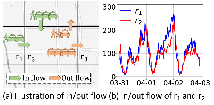
Figure 1: Illustration of close relationship between multiple spatio-temporal properties and regions.

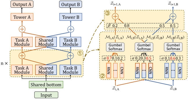
Figure 2: Model framework. The left part is the architecture of AutoSTL. From bottom to top, the model consists of shared bottom, $n$ hidden layers and task-specific tower. ① represents the hidden layer. The right part is the illustration of hidden layer, which consists of task-specific and shared modules ② and module fusion mechanism ③.

Researchers have been paying growing attention to Spatio-Temporal Multi-Task Learning (STMTL). The earliest attempt employs convolutional neural network to model the traffic flow and on-demand flow (Zhang et al. 2019). LSTM-based method was also incorporated to predict traffic in flow and out flow simultaneously (Zhang et al. 2020). However, there are several limitations for existing STMTL methods. Firstly, relationship between different tasks has not been well-addressed. Current STMTL methods basically employ MLP fusion layer or concatenation to fuse different task features. Secondly, in order to adapt to multiple properties, these methods are specified with manually designed module and architecture such as stacked LSTM or CNN, which may not be optimal for the complex task correlation and introduce human error. Last, existing methods aim to fixed combination of tasks, which suffer from poor transferability and scalability. It demands reconstruction with tremendous expert efforts for other tasks or data.

In this paper, we propose a self-adaptive architecture, named AutoSTL, to solve multiple spatio-temporal tasks simultaneously. We mainly face several serious challenges. First, the spatio-temporal correlations of all grids are complex to be well-captured, especially modeling multiple spatio-temporal properties. Besides, to benefit each specific task, it demands exploiting their entangled relationship and an appropriate feature fusion mechanism. Furthermore, in order to support flexible multiple task combinations, the model is supposed to be scalable and easily extendable. Finally, manually-designed model requires tremendous expert efforts and may trigger bias or mistakes, leading to a sub-optimal model. To fully address the problems above, we design a scalable architecture AutoSTL, which can automatically allocate modules with a set of advanced spatio-temporal operations. We introduce shared modules to specifically address the relationship between properties and an automated fusion mechanism to fuse multi-task features. The architecture consists of stacking hidden layers, where the modules inside and the fusion weight are fully self-adaptive. The main contributions could be summarized as follows:

• We propose a novel end-to-end framework, AutoSTL, to solve multiple spatio-temporal tasks simultaneously. It can automatically choose the suitable saptio-temporal module and fusion weight with trivial cost.

• A shared module modeling relationship between multiple tasks is incorporated, which can well-exploit the intrinsic dependency and benefit every single task.

• Our proposed model AutoSTL is the first model solving spatio-temporal multi-task learning automatically. Extensive experiments with multiple multi-task settings verified its efficacy and generality.

Preliminaries

Problem Definition. Spatio-Temporal Multi-Task Prediction. Let a graph $\boldsymbol{\mathcal{G}}=(\boldsymbol{\mathcal{V}},\boldsymbol{\mathcal{E}})$ describe the traffic state data. $\boldsymbol{\mathcal{V}}$ is the node set representing regions of city, and $\boldsymbol{\mathcal{E}}$ is the edge set which depicts the connectivity between regions. At time step $t$, the multi-task feature matrix of $\boldsymbol{\mathcal{G}}$ is $\boldsymbol{X}_{t}=$ [$\boldsymbol{x}_{t,1},...,\boldsymbol{x}_{t,k},...,\boldsymbol{x}_{t,K}$] $\in$ $\boldsymbol{R}^{N\times K}$, where $N$ is the number of region, $K$ is the number of task, and $k=1,...,K$ represents certain spatio-temporal task such as traffic speed, flow and trip duration of regions.

Spatio-temporal Multi-Task prediction aims to predict future multiple traffic states simultaneously given the historic states, by capturing the spatial and temporal variation pattern. The mapping function ${f_{\boldsymbol{W}}}$ parameterized by $\boldsymbol{W}$ is:

$$\boldsymbol{x}_{1:T,k},\boldsymbol{\mathcal{G}}\stackrel{{\scriptstyle f_{\boldsymbol{W}}}}{{\longrightarrow}}\boldsymbol{y}_{k},\forall k=1,...,K$$ (1)

where $\boldsymbol{x}_{1:T,k}$ $\in$ $\boldsymbol{R}^{T\times N}$ indicates the traffic state of historical $T$ time steps. $\boldsymbol{y}_{k}$ $\in$ $\boldsymbol{R}^{N}$ is the traffic state of task $k$ in the future time step. For convenient description, we omit the subscript and denote $\boldsymbol{X}_{1:T}$ as $\boldsymbol{X}$.

Methodology

Architecture Overview

We propose a scalable architecture to solve multiple spatio-temporal tasks in an automated way, named AutoSTL. As visualized in Figure 2, AutoSTL generally consists of shared bottom, hidden layers and task-specific tower.

We employ scalable hidden layer to capture spatio-temporal dependency of multiple tasks simultaneously. Specifically, we incorporate task-specific module to model each property and shared module to capture the intrinsic relationship between tasks. For module design, we define a spatio-temporal operation set including recurrent neural network, convolution neural network, graph convolution network and Transformer. The concrete assignation is searched by Automated Machine Learning (AutoML). For a further flexible fusion of multiple task properties, we propose self-adaptive fusion weights and optimize with AutoML. After representation learning of hidden layers, the task-specific tower predict by feeding on the multiple task features.

It is noteworthy that the module operations and fusion weights of AutoSTL are automatically decided. The optimal allocation contributes to effectively capturing spatio-temporal patterns of specific task and intrinsic relationships between multiple spatio-temporal tasks.

Framework

Shared Bottom

We transform the input data with an MLP layer shared bottom. Specifically, we input the feature matrix of historic $T$ time steps $\boldsymbol{X}$, and let $\boldsymbol{\mathcal{Z}}_{0}$ represent the hidden representation learned by the shared bottom.

$$\boldsymbol{\mathcal{Z}}_{0}=\sigma(\boldsymbol{W}_{s}\boldsymbol{X}+\boldsymbol{b}_{s})$$ (2)

where $\boldsymbol{W}_{s}$ and $\boldsymbol{b}_{s}$ represent weight and bias of MLP layer respectively, and $\sigma$ is activation function.

Hidden Layer

We employ $n$ stacking hidden layers to capture the spatio-temporal dependency of each task and the intrinsic relationship between different tasks. As shown in Figure 2, a hidden layer includes modules and fusion mechanism. We incorporate task-specific module for each task to address spatio-temporal dependency, and shared module to address the intrinsic relationship between different tasks. For each module, we exploit a spatio-temporal operation set, and adaptively select one spatio-temporal operation from the operation set. Processed by the spatio-temporal operations, the features are flexibly fused by module fusion mechanism.

Spatio-Temporal Operation Set

We maintain a spatio-temporal operation set including multiple spatio-temporal operations to support the automatic assignment of module operations. Specifically, we employ diffusion convolution (Li et al. 2018), 1-D dilated causal convolution (Wu et al. 2019), long-short term memory (LSTM), informer (Zhou et al. 2021) and spatial-informer (Wu et al. 2021) as spatio-temporal data mining operations, abbreviated as GCN, CNN, RNN, TX, and TX_S, respectively.

Diffusion convolution has an edge on capturing spatial dependency in data. In particular, it characterizes graph convolution based on $K$-step random walking on the graph. The diffusion convolution on the hidden representation is:

$$\!\mathcal{O}_{GCN}\!(\boldsymbol{\mathcal{Z}}_{i})\!=\!\sum_{k=0}^{K}\!\left(\boldsymbol{D}_{O}^{-1}\!\boldsymbol{A}\right)^{k}\!\boldsymbol{\mathcal{Z}}_{i}\!\boldsymbol{W}_{1,k}\!+\!\left(\!\boldsymbol{D}_{I}^{-1}\!\boldsymbol{A}^{\top}\!\right)^{k}\!\boldsymbol{\mathcal{Z}}_{i}\!\boldsymbol{W}_{2,k}$$ (3)

where $\boldsymbol{A}$ is the adjacent matrix of $\boldsymbol{\mathcal{G}}$, $\boldsymbol{D}_{O}^{-1}$ and $\boldsymbol{D}_{I}^{-1}$ are out-degree and in-degree diagonal matrices. $\boldsymbol{W}_{1,k}$ and $\boldsymbol{W}_{2,k}$ are trainable filter parameters.

1-D dilated causal convolution is an effective operation for temporal information. Through padding zero to input data, it reserves causal temporal dependency and is able to predict next state based on past states (Wu et al. 2019).

$$\mathcal{O}_{CNN}(\boldsymbol{\mathcal{Z}}_{i})=\left(\boldsymbol{\mathcal{Z}}_{i}\boldsymbol{W}_{3}\right)\odot\sigma\left(\boldsymbol{\mathcal{Z}}_{i}\boldsymbol{W}_{4}\right)$$ (4)

LSTM is a classical technique to learn temporal information. It enjoys a naturally-progressive architecture to model the sequential dependency and predict the future state. It is generally-applied in spatio-temporal data mining methods (Zhang et al. 2016; Zhang, Zheng, and Qi 2017).

$$\mathcal{O}_{RNN}(\boldsymbol{\mathcal{Z}}_{i})=LSTM(\boldsymbol{\mathcal{Z}}_{i})$$ (5)

Transformer has proven its efficacy in recent spatio-temporal prediction advances (Guo et al. 2019; Li et al. 2019), we employ its efficient variant informer (Zhou et al. 2021), and the enhanced version spatial-informer considering spatial dependency (Wu et al. 2021) as operations, i.e., TX and TX_S. TX could be formulated as follows:

$$\mathcal{O}_{TX}\!=\!{softmax}\bigg{(}\!\frac{\psi\big{(}\boldsymbol{\mathcal{Z}}^{(i)}\boldsymbol{W}_{Q}\big{)}\big{(}\boldsymbol{\mathcal{Z}}^{(i)}\boldsymbol{W}_{K}\big{)}^{\top}}{\sqrt{d}}\!\bigg{)}\big{(}\boldsymbol{\mathcal{Z}}^{(i)}\boldsymbol{W}_{V}\big{)}$$ (6)

where $\psi$ is the sampling function in informer, $d$ is feature dimension, and $\boldsymbol{W}_{Q}$, $\boldsymbol{W}_{K}$, $\boldsymbol{W}_{V}$ are trainable weight matrices. Similarly, spatial-informer conducts attention mechanism on spatial relationship, i.e., $\mathcal{O}_{TX\_S}$ feeds on the spatial transposition of $\boldsymbol{\mathcal{Z}}_{i}$.

Based on the spatio-temporal operations, we attain the operation set $\boldsymbol{\mathcal{O}}$ = [$\mathcal{O}_{GCN}$, $\mathcal{O}_{RNN}$, $\mathcal{O}_{CNN}$, $\mathcal{O}_{TX}$, $\mathcal{O}_{TX\_S}$]. As in bottom right of Figure 2, operations in each module are from $\boldsymbol{\mathcal{O}}$. It is worth noting that the spatio-temporal operation set is extensible. We select operations due to their advanced capacity of modeling spatial and temporal dependency as well as efficiency. The operation set could be easily modified or extended for future potential enhancement.

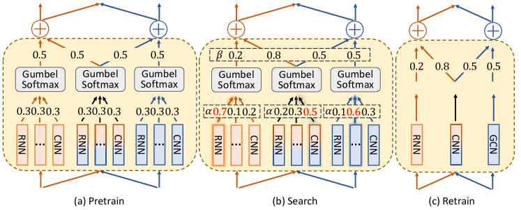
Figure 3: Three phases of weights searching. (a). Pretrain architecture, weights are fixed as initialization. (b). Search optimal weights by AutoML. (c). Identify operation in modules and achieve the optimal architecture.

Task-specific and Shared Module

As visualized in Figure 2, we present two kinds of modules in hidden layer, i.e., task-specific module and shared module. Task-specific module aims to capture information benefiting a certain task, and shared module is supposed to learn the entangled correlation between different tasks. Note that in each hidden layer, we can assign multiple task-specific modules and shared modules. For clear description, we assign one task-specific module for each task as well as one shared module in each hidden layer, as shown in Figure 2. We denote the module of layer $i$ as $\mathcal{M}_{i,\lambda}$, where $\lambda$$\in$ {A,B,S}. $\lambda=S$ stands for shared module, and $\lambda=A$ and $B$ represent task-specific module of task A and B, respectively. For instance, $\mathcal{M}_{2,A}$ is the specific module of task A in the $2$-nd hidden layer.

To maintain a trade-off between efficacy and efficiency, we search one specific operation for each module, rather than utilize all operations. There emerges a challenge that the hard selection of operations can not be optimized with gradient due to the non-differentiable selection. Conventionally, a soft weight $\boldsymbol{\alpha}$ is added to depict the significance of candidate operations, and a soft fusion is hired to approach the selection. But it can hardly avoid reaching the sub-optimal result. To overcome this, we incorporate gumbel-softmax to approximate the hard selection of operations.

To identify operation in module, we assign weight for each module $\boldsymbol{\alpha}=$ [$\alpha^{GCN}$, $\alpha^{RNN}$, $\alpha^{CNN}$, $\alpha^{TX}$, $\alpha^{TX\_S}$] to weight all candidate operations. Then the operations of module could be identified through hard sampling by gumbel-max technique (Gumbel 1954). For instance, the module of the task A $\mathcal{M}_{i,A}(\boldsymbol{\mathcal{Z}}_{i,A})$ could be reached by:

$$\mathcal{M}_{i,A}(\boldsymbol{\mathcal{Z}}_{i,A})\!=\!one\_{hot}\left(\underset{j\in[1,|\boldsymbol{\mathcal{O}}|]}{argmax}\left[\log\alpha_{j}+g_{j}\right]\right)\odot\boldsymbol{\mathcal{O}}(\boldsymbol{\mathcal{Z}}_{i})$$ (7)

where $g_{j}=-log(-log(\varepsilon_{j}))$ and $\varepsilon_{j}$ belongs to uniform distribution. $\odot$ is the dot product.

Due to the non-differentiable argmax operation, we introduce Gumbel-softmax (Jang, Gu, and Poole 2016; Zhao et al. 2021a). In particular, it simulates hard selection based on reparameterization on categorical distribution:

$$p_{j}=\frac{\exp\left(\left(\log\left(\alpha_{j}\right)+g_{j}\right)/\tau\right)}{\sum_{k=1}^{n}\exp\left(\left(\log\left(\alpha_{k}\right)+g_{k}\right)/\tau\right)}$$ (8)

where $p_{j}$ is the probability of selecting the operation $j$, and $\tau$ controls the approach to hard selection. When $\tau$ approaches to zero, the Gumbel-softmax outputs one-hot vector.

Module Fusion Mechanism

In order to model both task-specific and cross-tasks information, we propose a flexible module fusion mechanism. Take task A as an example, we fuse the output of its task-specific module $\mathcal{M}_{i,A}$ and shared module $\mathcal{M}_{i,S}$, and obtain the task-specific feature $\boldsymbol{\mathcal{Z}}_{i+1,A}$. Then, we output the task-specific feature to the task-specific and shared-modules in the next hidden layer. To dynamically weight each module’s contribution to the output, we set the fusion weight $\boldsymbol{\beta}=[\boldsymbol{\beta}_{A},\boldsymbol{\beta}_{B}]$ and search through gradient. So the task-specific feature of task A and B learned by the $(i+1)$-th layer $\boldsymbol{\mathcal{Z}}_{i+1,A}$ and $\boldsymbol{\mathcal{Z}}_{i+1,B}$ are as follows, which is illustrated in Figure 2:

$$\boldsymbol{\mathcal{Z}}_{i+1,A}=softmax(\boldsymbol{\beta}_{A})\odot[\mathcal{M}_{i,A}(\boldsymbol{\mathcal{Z}}_{i,A}),\mathcal{M}_{i,S}(\boldsymbol{\mathcal{Z}}_{i,A})]$$ (9)

$$\boldsymbol{\mathcal{Z}}_{i+1,B}=softmax(\boldsymbol{\beta}_{B})\odot[\mathcal{M}_{i,B}(\boldsymbol{\mathcal{Z}}_{i,B}),\mathcal{M}_{i,S}(\boldsymbol{\mathcal{Z}}_{i,B})]$$ (10)

Notably, the input of both tasks of the first hidden layer is $\boldsymbol{\mathcal{Z}}_{0}$. As shown in the left bottom of Figure 2, the output of shared bottom are duplicated and input to the first hidden layer, and the intermediate hidden layers feed on task specific features. The task-specific data output by the last hidden layer goes through task-specific tower and achieves the prediction of each task.

Task-specific Prediction Tower

After representation learning of $n$ hidden layers, we utilize task-specific tower to predict the future state. We hire MLP layers as tower, which enjoys low computational complexity.

$$\boldsymbol{Y}_{A}=\boldsymbol{W}_{oA}(\boldsymbol{\mathcal{Z}}_{n,A})+\boldsymbol{b}_{oA}$$ (11)

$$\boldsymbol{Y}_{B}=\boldsymbol{W}_{oB}(\boldsymbol{\mathcal{Z}}_{n,B})+\boldsymbol{b}_{oB}$$ (12)

where $\boldsymbol{W}_{oA}$ and $\boldsymbol{b}_{oA}$ are the weight matrix and bias of the tower of task A, so do $\boldsymbol{W}_{oB}$ and $\boldsymbol{b}_{oB}$ to task B.

Dataset	NYC Taxi								PEMSD4
Metrics	RMSE		MAE		RMSE		MAE		RMSE		MAE
Methods	In	Out	In	Out	OD	Duration	OD	Duration	Flow	Speed	Flow	Speed
ARIMA	23.63	25.36	13.81	13.87	1.04	3.21	0.84	2.01	146.01	8.37	114.51	4.40
DCRNN	7.75	7.21	4.73	4.58	0.63	3.09	0.25	1.52	27.67	2.06	17.42	1.11
GWNet	8.89	7.27	5.37	4.60	0.60	2.90	0.23	1.24	30.61	2.27	19.62	1.28
CCRNN	8.04	7.35	4.87	4.52	0.61	2.97	0.23	1.40	28.13	2.07	17.81	1.14
PLE	8.77	8.46	5.29	5.19	0.66	3.05	0.27	1.44	30.14	2.25	19.24	1.29
PLE-LSTM	8.66	8.31	5.19	5.09	0.65	3.04	0.27	1.38	29.60	2.11	18.66	1.20
DCRNN-MTL	7.85	7.52	4.84	4.75	0.62	2.92	0.24	1.28	27.65	2.34	17.44	1.46
CCRNN-MTL	7.68	7.50	4.62	4.53	0.63	2.86	0.24	1.22	27.99	2.56	17.59	1.52
GTS†	7.86	7.40	4.90	4.65	-	-	-	-	28.05	2.09	17.87	1.15
MTGNN	7.64	7.17	4.67	4.48	0.59	2.89	0.24	1.24	28.03	2.05	17.92	1.12
AutoSTL	7.57*	7.16	4.53*	4.41*	0.59	2.89	0.21*	1.12*	27.36*	2.01*	17.40*	1.08*

†GTS fails to run on traffic OD flow and trip duration due to its tremendous allocation of GPU space.

Table 1: Overall experiment results. Best performances are bold, next best performances are underlined. “*” indicates the statistically significant improvements (i.e., two-sided t-test with $p<0.05$) over the best baseline.

Optimization by AutoML

Traditional spatio-temporal prediction works endeavor to manually design specified architecture, which highly depends on expert’s experience and suffers from poor generality. AutoML has demonstrated its efficiency and efficacy on searching model operation and architecture with advanced model capacity (Pan et al. 2021; Wu et al. 2021; Zhao et al. 2021b). We utilize AutoML to maintain self-adaptive model architecture as well as module operations.

The optimization procedure consists of 3 phases, i.e., pretrain, search and retrain, as shown in Figure 3. First, we initialize and fix all searching weights $\boldsymbol{\alpha}$ and $\boldsymbol{\beta}$ as average value, and pretrain the model for several epochs. Then, we update $\boldsymbol{\alpha}$ and $\boldsymbol{\beta}$ with a mini-batch of validation data along with the model training, i.e., Bi-level Optimization. Finally, after the search phase, the optimal operations in module and weight of fusion mechanism are already identified. We retrain the optimal architecture with a full-training.

Bi-level Optimization

In AutoSTL, the concrete operations of modules in hidden layer and fusion weight are identified adaptively based on model training. AutoML will offer the model with optimal performance within the search space. Let $\boldsymbol{W}$ represent the neural network parameters of the AutoSTL, $\boldsymbol{\alpha}$ and $\boldsymbol{\beta}$ stand for the operations in modules and fusion weights, respectively. The whole algorithm could be optimized with a bi-level optimization. Notably, the update of architecture parameters $\boldsymbol{\alpha}$ and $\boldsymbol{\beta}$ are based on a mini-batch of validation data, which avoids overfitting problem with an acceptable computational cost:

$$\min_{\boldsymbol{\alpha},\boldsymbol{\beta}}\mathcal{L}_{val}\left(\boldsymbol{W}^{*}(\boldsymbol{\alpha},\boldsymbol{\beta}),\boldsymbol{\alpha},\boldsymbol{\beta}\right)$$ (13)

$$\text{ s.t. }\boldsymbol{W}^{*}(\boldsymbol{\alpha},\boldsymbol{\beta})=\arg\min_{\boldsymbol{W}}\mathcal{L}_{train}\left(\boldsymbol{W},\boldsymbol{\alpha}^{*},\boldsymbol{\beta}^{*}\right)$$

To alleviate the computational cost of the optimization of $\boldsymbol{W}^{*}(\boldsymbol{\alpha},\boldsymbol{\beta})$, we propose to approximate the inner optimization function with one step of gradient descent:

$$\boldsymbol{W}^{*}(\boldsymbol{\alpha},\boldsymbol{\beta})\approx\boldsymbol{W}-\eta\partial_{\boldsymbol{W}}\mathcal{L}_{train}(\boldsymbol{W},\boldsymbol{\alpha},\boldsymbol{\beta})$$ (14)

where $\eta$ is learning rate. Through iteratively minimizing training loss $\mathcal{L}_{train}$ and validation loss $\mathcal{L}_{val}$, we can achieve a model with the optimal performance.

Experiment

In this section, we present the experiment result as well as analysis to verify the efficacy of our proposed AutoSTL.

Datasets

We evaluate AutoSTL on two commonly used real-world benchmark datasets of spatio-temporal prediction, i.e., NYC Taxi and PEMSD4. We collect data from April to June in 2016 for NYC Taxi with 35 million trajectories, and the data of January and February in 2018 for PEMSD4.

Data Preprocessing

To thoroughly prove the capability of AutoSTL on STMTL, we propose multiple experimental scenarios with different datasets. In a nutshell, we execute two groups of multi-task on NYC Taxi, i.e., traffic in flow and out flow, as well as traffic on-demand flow and trip duration. Besides, we propose one multi-task setting on PEMSD4, i.e., traffic flow and speed of sensors on road.

Baselines

We compare with two lines of representative spatio-temporal prediction methods, which can be grouped as methods for single task and multiple tasks. Methods for single task: ARIMA (Box et al. 2015), DCRNN (Li et al. 2018), GWNet (Wu et al. 2019), CCRNN (Ye et al. 2021). Methods for multiple tasks: PLE (Tang et al. 2020), PLE-LSTM , DCRNN-MTL, CCRNN-MTL, MTGNN (Wu et al. 2020), GTS (Shang and Chen 2021).

Experimental Setups

To facilitate the reproducibility, we detail the experimental setting including training environment and implementation details. We predict the traffic attribute of the future 1 time interval based on the historical 12 time steps, i.e., $|T|=12$. We select root mean squared error (RMSE) and mean absolute error (MAE) as evaluation metrics. All experimental results are the average value of 5 individual runs.

In terms of model structure, we assign 1 task-specific module and 1 shared module in each hidden layer, e.g., 3 modules in one hidden layer for two-tasks learning. We stack 3 hidden layers in total.

Overall Performance

Table 1 presents the overall experiment results. From the result we can exactly reach conclusions below: In the group of the method for single-task, (1) ARIMA gets worse results than deep learning-based models in all tasks. The performance gap is because of the advanced capacity of neural networks. (2) DCRNN and GWNet take the leading place among the GCN-based methods, and DCRNN performs steadily on different datasets. The possible reason is that the adaptive adjacent matrix equipped with GWNet and CCRNN makes the performance unstable. (3) AutoSTL outperforms single task baselines consistently, including the state-of-the-art spatio-temporal prediction methods, i.e., DCRNN, GWNet, and CCRNN. It verifies AutoSTL the advanced ability of capturing spatio-temporal dependency between different properties, which benefits each single task and attains the best performance.

Among the multi-task methods, (1) PLE-LSTM performs better than PLE, which shows the capability of LSTM for modeling temporal dependency beyond MLP. (2) DCRNN-MTL and CCRNN-MTL did not achieve better results than their single-task setting. This is a seesaw phenomenon that model improves the performance of one task but hurts the other one, which commonly emerges in multi-task learning and is ascribed to the incapability of modeling multiple properties. (3) AutoSTL achieves superior results than GTS and MTGNN, the latter two are designed specifically for modeling multi-variate time series. It verifies the efficacy of the self-adaptive architecture and operations in AutoSTL. (4) AutoSTL attains consistently advanced performance while baseline models achieve fluctuant results on different tasks and datasets. The flexible spatio-temporal operation and the automatic allocation by AutoML contribute to the outstanding adaptivity to different tasks and datasets.

Methods	RMSE		MAE
	In	Out	In	Out
w/o $\boldsymbol{\alpha}$	7.77	7.20	4.65	4.44
w/o $\boldsymbol{\beta}$	7.94	7.47	4.75	4.59
w/o s-m	9.13	7.22	5.69	4.51
AutoSTL	7.57	7.16	4.53	4.41

Table 2: Components analysis of AutoSTL on NYC Taxi.

Ablation Study

In this subsection, we present several variants of our proposed method and make a detailed comparison with them to verify the effective components in AutoSTL.

• w/o $\boldsymbol{\alpha}$: Fix operations in hidden layers with optimal ones.

• w/o $\boldsymbol{\beta}$: Fix fusion weights with average value.

• w/o s-m: Remove shared module in hidden layer.

Table 2 presents the results of AutoSTL and the variants. From the result, we can safely draw conclusions as follows: (1) Based on the experiment result on NYC Taxi, we fix the operations of 3 hidden layers with GCN, GCN and RNN from bottom to top, which is a proper approximation to the manual-design model. According to the results, we find that the specific operation allocation inside each hidden layer still affects the performance, and the automated architecture, i.e., AutoSTL, performs better. (2) Through fixing the fusion weights $\boldsymbol{\beta}$ and considering the equal contribution of each module in the hidden layer, we test the function of the self-adaptive fusion mechanism. The results demonstrate the prominence of properly weighting different spatio-task features. (3) By removing the shared module in each hidden layer, we test its contribution to multi-task learning.

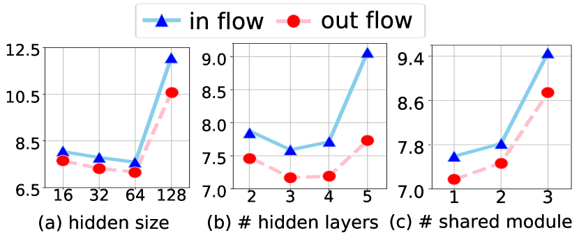
Figure 4: Influence of hyper-parameters on NYC Taxi dataset. We present the RMSE of traffic in and out flow.

The distinct performance gap below AutoSTL proves the advanced ability to address the dependency of the shared module. Without effectively modeling the relationship between multiple tasks, w/o s-m converges with optimizing single task, i.e., traffic out flow, whereas performs considerably less well in traffic in flow prediction.

Hyper-parameter Analysis

We demonstrate how hyper-parameters influence the performance of AutoSTL. We verify the key hyper-parameters, i.e., the hidden size of embedding layer, the number of hidden layers and the number of shared module in hidden layer.

Figure 4 presents the RMSE performance of traffic in and out flow on NYC Taxi dataset. In Figure 4(a), we test hidden size in {16, 32, 64, 128}. An improvement of hidden size in a relatively-low range can benefit performance, but when it is too large, i.e., 128, the model collapses dramatically, which is possibly caused by overfitting problem. From Figure 4(b), AutoSTL with 3 hidden layers achieves best performance, fewer hidden layer impairs model capacity, while large ones may trigger overfitting. As shown in Figure 4(c), we can conclude that only 1 shared module in each hidden layer is enough for multiple properties modeling.

Efficiency Comparison

We compare parameter volume, training time, and inference time on NYC Taxi in Table 3. For AutoSTL, it contains 3 phases, i.e., pretrain, search and retrain. In pretrain and search phases, the model has 142K parameters, and the final searched model has 312K for retrain phase. Following Wu et al. (Wu et al. 2021), we set the embedding size of the first two phases a quarter of that of the retrain phase, so the pretrain and search phases have fewer parameters and take trivial training costs, i.e., about one-seventh training cost of model retraining. From the results, we can observe that AutoSTL achieves state-of-the-art prediction effectiveness with competitive space and time consumption. MTGNN takes less training time than AutoSTL, but it demands twice space allocation due to its MLP components.

Visualization

We show the efficacy of AutoSTL from multiple views. Figure 5 illustrates the validation loss of traffic in flow on NYC Taxi with respect to training epoch. We can observe that AutoSTL converge with least epochs, i.e., 32, while all baselines take at least 70 epochs to converge. AutoSTL hires advanced spatio-temporal operations into a compact architecture, which leads to more accurate gradient descent, and fosters quicker convergence with fewer training epochs.

Methods	MAE		Para	Training	Inference
	In	Out	(K)	time(s)	time(ms)
DCRNN	4.73	4.58	127	11,556	1280
GWNet	5.37	4.60	272	2,056	40
CCRNN	4.87	4.52	139	2,218	53
DCRNN-MTL	4.84	4.75	127	5,783	1280
CCRNN-MTL	4.62	4.53	139	1,236	52
MTGNN	4.67	4.48	612	1683	78
AutoSTL	4.53	4.41	312	1,958	100

Table 3: Space and time efficiency comparison.

Related Work

Traditional Spatio-Temporal Prediction

Varieties of deep learning techniques have been applied to spatio-temporal prediction. The capability of deep learning techniques can be roughly divided into two categories, i.e., temporal pattern capture and spatial pattern capture. For temporal pattern capture, since Ma et al. (Ma et al. 2015) and Tian et al. (Tian and Pan 2015) first applied LSTM to spatio-temporal prediction, there emerge a bunch of Recurrent Neural Network (RNN) methods such as LSTM and GRU capturing the temporal variation pattern (Ma et al. 2015; Tian and Pan 2015; Li et al. 2018). Also, 1-D Convolution (Guo et al. 2019) and its enhancement with Dilated Causal Convolution (Yu, Yin, and Zhu 2018; Yu and Koltun 2015) have also achieved good performance with outstanding efficiency. For spatial pattern capture, DeepST (Zhang et al. 2016) and ST-ResNet (Zhang, Zheng, and Qi 2017) are representative efforts made to enhance RNN with CNN to respectively model the temporal and spatial correlation. Besides, STGCN (Yu, Yin, and Zhu 2018) and DCRNN (Li et al. 2018) firstly propose to describe spatial relationship in spatio-temporal prediction with graph structure. Our AutoSTL framework hires a spatio-temporal operation set with advanced and efficient spatio-temporal operations, and assigns operation automatically, which considers spatial and temporal dependency comprehensively.

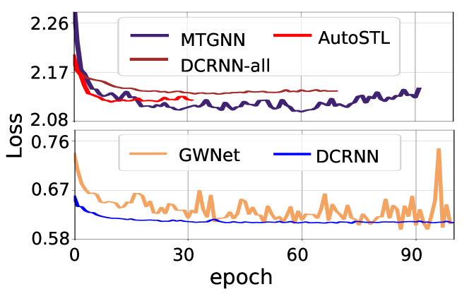
Figure 5: Loss curves comparison on NYC Taxi.

Spatio-temporal Multi-Task Learning

Spatio-temporal multi-task learning methods could be referred to two main lines of researches, i.e., spatio-temporal multi-task learning and multi-variate time series prediction. For spatio-temporal multi-task learning, MDL (Zhang et al. 2020) is one of the earliest endeavours, which incorporates convolutional neural network to solve traffic node flow and edge flow jointly. Zhang et al. propose a full LSTM method to predict traffic in and out flow together (Zhang et al. 2019). Other STMTL works includes MasterGNN (Han et al. 2021), MT-ASTN (Wang et al. 2020), GEML (Wang et al. 2019), etc. These models are restricted to solving two specific tasks and suffer from poor generality. For multi-variate time series prediction, MTGNN hires graph neural network for multivariate time series data prediction (Wu et al. 2020). DMVST-Net (Yao et al. 2018) consider multivariate time series in temporal, spatial and semantic views. GTS (Shang and Chen 2021) incorporates a probabilistic graph model and achieves an efficient approach for graph structure learning. This line of models demand human efforts for new settings due to the highly-specified architecture. Our AutoSTL is the first attempt to handle flexibly multiple spatio-temporal tasks. Its multi-task framework and shared module well exploit the attributes’ relationship. Besides, it assigns modules and hyperparameters automatically for different settings and achieves good generality.

Conclusion

In this paper, we present a self-adaptive framework to model multiple spatio-temporal tasks effectively. We present a spatio-temporal operation set as candidate operation. A scalable architecture consisting of extendable hidden layers is proposed, where each layer is composed of task-specific and shared modules. To further enhance the multi-task learning, we employ a fusion mechanism to fuse multiple task features. In order to support flexible combinations of multiple tasks and data, we assign operations in module and fusion weight by AutoML. Our proposed method is the first to solve spatio-temporal multi-task learning automatically.

In terms of the physical application of spatio-temporal prediction in today’s life, our method could be easily extended to other domains such as weather and environment, public safety, human mobility, etc. In the future, we will continue discovering its potential efficacy on more applications.

References

- Box et al. (2015) Box, G. E.; Jenkins, G. M.; Reinsel, G. C.; and Ljung, G. M. 2015. Time series analysis: forecasting and control. John Wiley & Sons.
- Caruana (1997) Caruana, R. 1997. Multitask learning. Machine learning, 28(1): 41–75.
- Chen et al. (2022) Chen, L.; Jia, N.; Zhao, H.; Kang, Y.; Deng, J.; and Ma, S. 2022. Refined analysis and a hierarchical multi-task learning approach for loan fraud detection. Journal of Management Science and Engineering, 7(4): 589–607.
- Cui et al. (2021) Cui, Q.; Zhang, C.; Zhang, Y.; Wang, J.; and Cai, M. 2021. ST-PIL: Spatial-Temporal Periodic Interest Learning for Next Point-of-Interest Recommendation. In Proceedings of the 30th ACM International Conference on Information & Knowledge Management, 2960–2964.
- Feng et al. (2021) Feng, S.; Ke, J.; Yang, H.; and Ye, J. 2021. A multi-task matrix factorized graph neural network for co-prediction of zone-based and od-based ride-hailing demand. IEEE Transactions on Intelligent Transportation Systems.
- Gumbel (1954) Gumbel, E. J. 1954. Statistical theory of extreme values and some practical applications: a series of lectures, volume 33. US Government Printing Office.
- Guo et al. (2016) Guo, H.; Li, X.; He, M.; Zhao, X.; Liu, G.; and Xu, G. 2016. CoSoLoRec: Joint Factor Model with Content, Social, Location for Heterogeneous Point-of-Interest Recommendation. In International Conference on Knowledge Science, Engineering and Management, 613–627. Springer.
- Guo et al. (2019) Guo, S.; Lin, Y.; Feng, N.; Song, C.; and Wan, H. 2019. Attention based spatial-temporal graph convolutional networks for traffic flow forecasting. In Proceedings of the AAAI conference on artificial intelligence, volume 33, 922–929.
- Han et al. (2021) Han, J.; Liu, H.; Zhu, H.; Xiong, H.; and Dou, D. 2021. Joint Air Quality and Weather Prediction Based on Multi-Adversarial Spatiotemporal Networks. In Proceedings of the 35th AAAI Conference on Artificial Intelligence.
- Jang, Gu, and Poole (2016) Jang, E.; Gu, S.; and Poole, B. 2016. Categorical reparameterization with gumbel-softmax. arXiv preprint arXiv:1611.01144.
- Li et al. (2019) Li, S.; Jin, X.; Xuan, Y.; Zhou, X.; Chen, W.; Wang, Y.-X.; and Yan, X. 2019. Enhancing the locality and breaking the memory bottleneck of transformer on time series forecasting. Advances in neural information processing systems, 32.
- Li et al. (2018) Li, Y.; Yu, R.; Shahabi, C.; and Liu, Y. 2018. Diffusion Convolutional Recurrent Neural Network: Data-Driven Traffic Forecasting. In International Conference on Learning Representations.
- Ma et al. (2015) Ma, X.; Tao, Z.; Wang, Y.; Yu, H.; and Wang, Y. 2015. Long short-term memory neural network for traffic speed prediction using remote microwave sensor data. Transportation Research Part C: Emerging Technologies, 54: 187–197.
- Pan et al. (2021) Pan, Z.; Ke, S.; Yang, X.; Liang, Y.; Yu, Y.; Zhang, J.; and Zheng, Y. 2021. AutoSTG: Neural Architecture Search for Predictions of Spatio-Temporal Graph*. In Proceedings of the Web Conference 2021, 1846–1855.
- Shang and Chen (2021) Shang, C.; and Chen, J. 2021. Discrete Graph Structure Learning for Forecasting Multiple Time Series. In Proceedings of International Conference on Learning Representations.
- Tang et al. (2020) Tang, H.; Liu, J.; Zhao, M.; and Gong, X. 2020. Progressive layered extraction (ple): A novel multi-task learning (mtl) model for personalized recommendations. In Fourteenth ACM Conference on Recommender Systems, 269–278.
- Tian and Pan (2015) Tian, Y.; and Pan, L. 2015. Predicting short-term traffic flow by long short-term memory recurrent neural network. In 2015 IEEE international conference on smart city/SocialCom/SustainCom (SmartCity), 153–158. IEEE.
- Wang et al. (2022) Wang, P.; Zhu, C.; Wang, X.; Zhou, Z.; Wang, G.; and Wang, Y. 2022. Inferring Intersection Traffic Patterns with Sparse Video Surveillance Information: An ST-GAN method. IEEE Transactions on Vehicular Technology.
- Wang et al. (2020) Wang, S.; Miao, H.; Chen, H.; and Huang, Z. 2020. Multi-task adversarial spatial-temporal networks for crowd flow prediction. In Proceedings of the 29th ACM international conference on information & knowledge management, 1555–1564.
- Wang et al. (2019) Wang, Y.; Yin, H.; Chen, H.; Wo, T.; Xu, J.; and Zheng, K. 2019. Origin-destination matrix prediction via graph convolution: a new perspective of passenger demand modeling. In Proceedings of the 25th ACM SIGKDD international conference on knowledge discovery & data mining, 1227–1235.
- Wu et al. (2021) Wu, X.; Zhang, D.; Guo, C.; He, C.; Yang, B.; and Jensen, C. S. 2021. AutoCTS: Automated correlated time series forecasting. Proceedings of the VLDB Endowment, 15(4): 971–983.
- Wu et al. (2020) Wu, Z.; Pan, S.; Long, G.; Jiang, J.; Chang, X.; and Zhang, C. 2020. Connecting the dots: Multivariate time series forecasting with graph neural networks. In Proceedings of the 26th ACM SIGKDD international conference on knowledge discovery & data mining, 753–763.
- Wu et al. (2019) Wu, Z.; Pan, S.; Long, G.; Jiang, J.; and Zhang, C. 2019. Graph WaveNet for Deep Spatial-Temporal Graph Modeling. In Proceedings of the Twenty-Eighth International Joint Conference on Artificial Intelligence, IJCAI-19, 1907–1913. International Joint Conferences on Artificial Intelligence Organization.
- Xu et al. (2016) Xu, T.; Zhu, H.; Zhao, X.; Liu, Q.; Zhong, H.; Chen, E.; and Xiong, H. 2016. Taxi driving behavior analysis in latent vehicle-to-vehicle networks: A social influence perspective. In Proceedings of the 22nd ACM SIGKDD International Conference on Knowledge Discovery and Data Mining, 1285–1294. ACM.
- Yao et al. (2018) Yao, H.; Wu, F.; Ke, J.; Tang, X.; Jia, Y.; Lu, S.; Gong, P.; Ye, J.; and Li, Z. 2018. Deep multi-view spatial-temporal network for taxi demand prediction. In Proceedings of the AAAI conference on artificial intelligence, volume 32.
- Ye et al. (2021) Ye, J.; Sun, L.; Du, B.; Fu, Y.; and Xiong, H. 2021. Coupled layer-wise graph convolution for transportation demand prediction. In Proceedings of the AAAI conference on artificial intelligence, volume 35, 4617–4625.
- Yu, Yin, and Zhu (2018) Yu, B.; Yin, H.; and Zhu, Z. 2018. Spatio-temporal graph convolutional networks: A deep learning framework for traffic forecasting. In International Joint Conferences on Artificial Intelligence Organization, 3634–3640.
- Yu and Koltun (2015) Yu, F.; and Koltun, V. 2015. Multi-scale context aggregation by dilated convolutions. arXiv preprint arXiv:1511.07122.
- Zhang et al. (2020) Zhang, C.; Zhu, F.; Wang, X.; Sun, L.; Tang, H.; and Lv, Y. 2020. Taxi demand prediction using parallel multi-task learning model. IEEE Transactions on Intelligent Transportation Systems.
- Zhang, Zheng, and Qi (2017) Zhang, J.; Zheng, Y.; and Qi, D. 2017. Deep spatio-temporal residual networks for citywide crowd flows prediction. In Thirty-first AAAI conference on artificial intelligence.
- Zhang et al. (2016) Zhang, J.; Zheng, Y.; Qi, D.; Li, R.; and Yi, X. 2016. DNN-based prediction model for spatio-temporal data. In Proceedings of the 24th ACM SIGSPATIAL international conference on advances in geographic information systems, 1–4.
- Zhang et al. (2019) Zhang, J.; Zheng, Y.; Sun, J.; and Qi, D. 2019. Flow prediction in spatio-temporal networks based on multitask deep learning. IEEE Transactions on Knowledge and Data Engineering, 32(3): 468–478.
- Zhao et al. (2022a) Zhao, C.; Zhao, H.; Wu, R.; Deng, Q.; Ding, Y.; Tao, J.; and Fan, C. 2022a. Multi-dimensional Prediction of Guild Health in Online Games: A Stability-Aware Multi-task Learning Approach.
- Zhao et al. (2022b) Zhao, X.; Fan, W.; Liu, H.; and Tang, J. 2022b. Multi-type Urban Crime Prediction. In Proceedings of the AAAI Conference on Artificial Intelligence, volume 36, 4388–4396.
- Zhao et al. (2021a) Zhao, X.; Liu, H.; Fan, W.; Liu, H.; Tang, J.; and Wang, C. 2021a. Autoloss: Automated loss function search in recommendations. In Proceedings of the 27th ACM SIGKDD Conference on Knowledge Discovery & Data Mining, 3959–3967.
- Zhao et al. (2021b) Zhao, X.; Liu, H.; Liu, H.; Tang, J.; Guo, W.; Shi, J.; Wang, S.; Gao, H.; and Long, B. 2021b. Autodim: Field-aware embedding dimension searchin recommender systems. In Proceedings of the Web Conference 2021, 3015–3022.
- Zhao and Tang (2017a) Zhao, X.; and Tang, J. 2017a. Exploring Transfer Learning for Crime Prediction. In 2017 IEEE International Conference on Data Mining Workshops (ICDMW), 1158–1159. IEEE.
- Zhao and Tang (2017b) Zhao, X.; and Tang, J. 2017b. Modeling Temporal-Spatial Correlations for Crime Prediction. In Proceedings of the 2017 ACM on Conference on Information and Knowledge Management, 497–506. ACM.
- Zhou et al. (2021) Zhou, H.; Zhang, S.; Peng, J.; Zhang, S.; Li, J.; Xiong, H.; and Zhang, W. 2021. Informer: Beyond efficient transformer for long sequence time-series forecasting. In Proceedings of the AAAI Conference on Artificial Intelligence, volume 35, 11106–11115.
- Zhou et al. (2020) Zhou, Z.; Wang, Y.; Xie, X.; Chen, L.; and Liu, H. 2020. RiskOracle: a minute-level citywide traffic accident forecasting framework. In Proceedings of the AAAI Conference on Artificial Intelligence, volume 34, 1258–1265.