A bilevel approach for compensation and routing decisions in last-mile delivery

Abstract

In last-mile delivery logistics, peer-to-peer logistic platforms play an important role in connecting senders, customers, and independent carriers to fulfill delivery requests. Since the carriers are not under the platform’s control, the platform has to anticipate their reactions, while deciding how to allocate the delivery operations. Indeed, carriers’ decisions largely affect the platform’s revenue. In this paper, we model this problem using bilevel programming. At the upper level, the platform decides how to assign the orders to the carriers; at the lower level, each carrier solves a profitable tour problem to determine which offered requests to accept, based on her own profit maximization. Possibly, the platform can influence carriers’ decisions by determining also the compensation paid for each accepted request. The two considered settings result in two different formulations: the bilevel profitable tour problem with fixed compensation margins and with margin decisions, respectively. For each of them, we propose single-level reformulations and alternative formulations where the lower-level routing variables are projected out. A branch-and-cut algorithm is proposed to solve the bilevel models, with a tailored warm-start heuristic used to speed up the solution process. Extensive computational tests are performed to compare the proposed formulations and analyze solution characteristics.

1 Introduction

The term “last-mile delivery” refers to the final leg in a Business-To-Consumer delivery service whereby the consignment is delivered to the recipient, either at the recipient’s home or at a collection point. A situation that is rather common nowadays in last-mile delivery systems is the one in which a platform receives orders from customers requiring a delivery (and collects the corresponding price for delivery), but delivery operations are performed by independent carriers who have spot contracts with the platform, and receive a compensation for each of them. The platform, therefore, decides how to allocate the orders to the carriers, and, possibly, the compensation margin to apply to each order. On the other side, carriers decide whether to accept the assignment from the platform. Indeed, such a situation is an alternative to existing approaches that consider only one decision maker, and applies to real-world routing applications in which there are different stakeholders who act according to their own objectives, which in turn might be conflicting. Clearly, the goal of the platform is maximizing its own profit. However, carriers also act on the base of their own profit maximization, and might possibly refuse to deliver orders assigned to them by the platform in case the corresponding compensation is too low. Thus, the platform has to anticipate carriers’ decisions in order to optimize its own profit. This sequential decision making process can be modeled using bilevel programming. The platform acts as a leader, getting a profit associated with each delivered order, corresponding to the price paid by the customer minus the compensation given to the carriers. At the lower level, each carrier maximizes the difference between the compensation offered by the platform on the orders assigned to her, and her own routing cost.

Problems of this type are faced in practice by the so-called peer-to-peer transportation platforms, which dynamically connect service (e.g., a ride, a delivery) requests with independent carriers that are not under the platform’s control. As a result, the platform cannot be sure that an offered request will be accepted by the service providers (carriers), who base their selection on their net profits. In some cases, the platform may influence the decisions of the carriers by selecting, not only the requests offered to each of them but also the compensation associated with each request.

Throughout this paper we assume that the carriers deliver all accepted orders in one single route, hence the lower-level problem faced by each driver corresponds to a Profitable Tour Problem (PTP). The PTP belongs to the class of Vehicle Routing Problems (VRPs) with profits. In PTP, a vehicle, starting from a central depot, can visit a subset of the available customers, collecting a specific profit whenever a customer is visited. The objective of the problem is the maximization of the net profit, i.e., the total collected profit minus the total route cost.

We consider two different settings for the studied problem: the Bilevel PTP with Fixed Margins (BPFM) and the Bilevel PTP with Margin Decisions (BPMD). The first setting models the case where the compensations paid to the carriers are fixed in advance. Thus, in this setting, at the upper level, a platform offers disjoint subsets of a given set of items (parcels/orders) to the set $K$ of carriers, while, at the lower level, each driver $k\in K$ solves a PTP and decides which items she accepts to serve. Both the platform and the carriers aim at maximizing their net profits, which are calculated differently at the two levels. The second setting models the case where the leader may influence the decisions of the carriers by deciding not only the sets of items to offer to each driver but the compensation paid for each of them as well. We propose two different bilevel formulations for the latter problem, and, for each of them, we solve the value function reformulation (in two versions) through a branch-and-cut approach. We further discuss the link between these two bilevel formulations, before comparing them computationally.

The contributions of this paper can be summarized as follows:

• We introduce the bilevel profitable tour problem with fixed compensation margins (i.e., BPFM), and with margin decisions (i.e., BPMD), where a platform acts as the leader who assigns customer orders to carriers, who act as followers; in the BPFM, the leader also defines the compensation for each item. With the BPMD, we fill the gap existing in the last-mile delivery literature regarding simultaneously considering upper-level compensation and lower-level routing decisions.

• We provide bilevel formulations for both problems, as well as their corresponding single-level reformulations. We start with the BPFM, and its formulation, properties, and single-level reformulation are used to introduce the more complex case, i.e., the BPMD. For this problem, we propose two alternative bilevel formulations, that are compared to prove that they provide equivalent bounds. For readers who are not familiar with bilevel optimization, which is at the core of our contribution, we present a brief introduction to this topic in Appendix A.

• We propose alternative formulations where the lower-level routing variables are either included or projected out.

• We develop a branch-and-cut algorithm for the solution of the BPMD where optimality, as well as feasibility cuts, are inserted dynamically. We also propose a warm-start Mixed-Integer Programming (MIP) heuristic to speed up the solution process. The heuristic is based on the solution of the BPFM under additional constraints.

• We perform extensive tests on instances adapted from benchmark instances for related problems to compare the different formulations we propose.

The paper is organized as follows. In Section 2 we revise the relevant literature. Section 3 introduces formally the problems under study as well as their mathematical formulations. Specifically, Section 3.1 focuses on the case where the margins are fixed, whereas Section 3.2 is devoted to the case where the margins are decision variables. In Section 3.3, we compare the two formulations proposed for the BPMD in Section 3.2. In Section 3.4 we derive new formulations by projecting out a set of variables from the upper-level formulation. In Section 4 the solution approaches for the proposed formulations are discussed. Section 5 describes the computational experiments and presents the numerical results. Finally, Section 6 concludes the paper.

2 Literature review

The study of peer-to-peer logistic platforms has experienced a significant increase in recent years. For a comprehensive overview, we address the readers to Agatz et al. (2012), Cleophas et al. (2019), Wang and Yang (2019), Le et al. (2019).

A wide literature on suppliers’ (carriers, drivers) selection in peer-to-peer logistic services either overlooked the behavior of suppliers, or assumed that their preferences are known in advance (sometimes together with a carrier’s bid on services (Kafle et al., 2017)). Sometimes, suppliers’ responses are assumed to be predeterminable: all suppliers will accept matches as long as they are stable (Wang et al., 2018) or meet some constraints, in the form, for example, of an upper bound on the extra driving time/distance (Masoud and Jayakrishnan, 2017, Arslan et al., 2019). More recently, the setting of peer-to-peer transportation platforms offering a menu of packages to occasional drivers, which we consider in the current work, has been addressed in Mofidi and Pazour (2019), Horner et al. (2021), Ausseil et al. (2022). As in our framework, the suppliers are not employed by the platform, thus the platform does not have perfect knowledge of the suppliers’ preferences related to which requests they would be willing to accept. In Mofidi and Pazour (2019), the platform decides the composition of multiple, simultaneous, personalized recommendations to the suppliers, who then select from this set. It is assumed that the platform is able to estimate the expected value of suppliers’ utility for each alternative assignment. A deterministic bilevel optimization model is thus presented, in which the platform takes as input the expectation of suppliers’ estimated utilities to make recommendation decisions. Horner et al. (2021) propose another bilevel formulation, based on the deterministic formulation presented in Mofidi and Pazour (2019), but adjusted by considering stochastic selection behaviors. A single-level relaxation is then proposed and a Sample Average Approximation method is used to optimize the expected value of the objective function over a sample of scenarios for the drivers’ behavior. Also Ausseil et al. (2022) consider a multiple scenario approach, repeatedly sampling potential drivers’ selections, solving the corresponding two-stage decision problems, and combining the multiple different solutions through a consensus function. Neither routing nor compensation decisions are taken into account in these models, which we instead consider in our paper. The deficiency in customized incentive systems, in particular, could potentially jeopardize the satisfaction of both the requester and the deliverer in terms of their utility and profit, respectively. This is implicitly highlighted in Horner et al. (2021), when stating that the proposed methods achieve good performances as long as the drivers are well compensated, i.e., when a percentage of 80% of the platform revenues goes to them. In support of this statement, Hong et al. (2019) propose a Stackelberg game to model the interaction between the platform, which decides both the delivery fees and the paths, and the drivers, who, based on the distance and their utility, make decisions about whether to participate in the delivery process or not. The computational experiments show that including decisions about compensation level in the process can significantly improve delivery efficiency, and reduce delivery costs compared to traditional delivery methods. In Gdowska et al. (2018), both a professional delivery fleet and a set of occasional carriers are taken into account. While the professional fleet is owned by the platform, the occasional carriers are independent, and can only deliver one parcel. Each delivery request has a fixed probability of being rejected by the occasional carriers. A compensation mechanism is considered to determine the fee to pay to each occasional driver in case a delivery request is accepted. Barbosa et al. (2023) extend the model introduced in Gdowska et al. (2018) by implementing a golden-section search method that determines the best compensation to offer for each request, considering the probability of rejection dependent on the compensation.

While compensation decisions have been optimized in a bilevel setting in some of the studies listed above, none of them explicitly models routing decisions at the lower level. In fact, an important feature of our approaches relies on the routing nature of the lower-level problem, and in the following, we review here works where bilevel optimization is used to model VRPs, as Du et al. (2017), Nikolakopoulos (2015), Parvasi et al. (2019), Marinakis and Marinaki (2008), Ning and Su (2017). All these works propose metaheuristics to solve the considered problems, and, more specifically, genetic algorithms. In Du et al. (2017), a multi-depot VRP is considered, and at the upper level, the assignment of customers to depots is decided, while depots-customers routing decisions are taken at the lower level. Nikolakopoulos (2015) address the VRP with backhauls and Time Windows, where a backhaul is a return trip to the depot, during which the vehicles pick up loads from the visited customers. The goal of the leader is to minimize the number of vehicles involved, whereas the follower aims to minimize the duration of the routes. A bilevel bi-objective formulation is proposed in Parvasi et al. (2019) to model the VRP where the involved vehicles are school buses. At the upper level, a transportation company selects some locations out of a set of potential bus stop locations (first objective) and determines the optimal bus routes among the selected stops (second objective). At the lower level, students are allocated to a stop or to another transportation company in order to minimize the time spent on buses. A bilevel location VRP is studied by Marinakis and Marinaki (2008). The upper level concerns decisions at the strategic level, i.e., the optimal locations of facilities. The lower level is about operational decisions regarding optimal vehicle routes. In Ning and Su (2017), a bilevel model is used to formulate the VRP with uncertain travel times. The leader aims at minimizing the waiting times of the customers, and the followers want to minimize those of the vehicles before the beginning of customers’ time windows. The uncertain bilevel model is reformulated into an equivalent deterministic one.

Calvete et al. (2011) consider a multi-depot VRP within a production–distribution planning problem. At the upper level, a distribution company orders from a manufacturing company the items that must be supplied to the retailers, while deciding on the allocation of such retailers (who play the role of customers) to each depot and on the routes that serve them. The manufacturing company, which is the follower, decides what manufacturing plants will produce the ordered items. Both players want to minimize their own costs. An ant colony optimization approach is developed to solve the bilevel model. The same conflicting agents are considered in Camacho-Vallejo et al. (2021), but with different objectives: the distribution company aims at maximizing the profit gained from the distribution process, and minimizing CO2 emissions; the manufacturer aims at minimizing its total costs. The upper level is thus a bi-objective problem. A tabu search heuristic is designed to obtain non-dominated feasible solutions for the distribution company. A hybrid algorithm combining ant colony optimization and tabu search is proposed in Wang et al. (2021) to solve a bilevel problem modeling the location-routing problem with cargo splitting, under four different low-carbon policies. The leader is the engineering construction department, which decides on the distribution center location. The follower takes the distribution department as the decision-maker to solve the VRP.

In Santos et al. (2021), a bilevel formulation is proposed to model the VRP with backhauls (without taking into account time windows considered in Nikolakopoulos (2015)). At the upper level, a shipper minimizes the transportation costs by integrating delivery and pickup operations in the routes; at the lower level a set of carriers, acting together, maximize their total net profit. The carriers, who may also serve requests from other shippers, may not be willing to collaborate with the shipper. To motivate the carriers to perform integrated routes, the shipper pays them an additional incentive. A reformulation is used to build an equivalent single-level problem.

In some cases, a bilevel approach has been proposed to address a routing problem even if the decision maker of both levels is the same. For instance, Marinakis et al. (2007) formulate the Capacitated VRP as a bilevel problem, where the first-level decisions concern the assignment of customers to the routes, and the second-level decisions determine the actual routes.

None of the works mentioned above deals with BPFM or BPMD so we now introduce a formal description of these problems.

3 Problems definition and formulations

In this section, we provide a formal description of the problems we address as well as the corresponding mathematical formulations. After introducing the notations we will use throughout the paper, as well as the two problems we address (BPFM and BPMD), we first focus on the problem with fixed compensation margins (Section 3.1) and then we move to the case where margins are decision variables (Section 3.2). In Section 3.3, we compare the two bilevel formulations proposed for BPMD in Section 3.2. In Section 3.4, we show how the introduced models can be modified by projecting out routing variables of the followers’ problem. Finally, in Section 3.5, we discuss how the proposed formulations change if the setting of the followers’ problem is modified by considering a maximum route duration constraint instead of a capacity constraint (measured as the maximum number of packages that can be delivered by each carrier).

Input sets and parameters

Sets and parameters used in the definition of the problems are listed below.

• $\mathcal{G}=(V,A)$: routing network over all nodes $V_{0}=\{0,\dots,n\}$; in particular, $V=V_{0}\setminus\{0\}$ corresponds to the set of customers to serve, and node $0$ to the depot where all routes start and end;

• $K$: index set of carriers/drivers/followers/vehicles;

• $p_{i}$: price that is paid to the platform if customer $i$ is served;

• $\bar{p}^{k}_{i}$: compensation paid by the platform to carrier $k$ if she accepts to serve customer $i$;

• $c^{k}_{ij}$: arc $\left(i,j\right)$ weight representing travel time for carrier $k$; we assume that arc weights $c^{k}_{ij}$ satisfy the triangle inequality;

• $b^{k}$: upper bound on the number of items the platform can assign to carrier $k$ ($b^{k}<n$ for all $k$);

• $t_{max}^{k}$: upper bound on the duration of the route for carrier $k$.

Notations

In the rest of this paper, we denote by $\delta^{+}(i)$ ($\delta^{-}(i)$) the set of arcs exiting from (entering) vertex $i$, and by $\mathcal{T}$ be the set of all routes in graph $\mathcal{G}=(V,A)$. Moreover, we denote by $T\in\mathcal{T}$ an arbitrary route, with $V(T)$ and $A(T)$ being the set of vertices and arcs visited and traversed by the route, respectively. Furthermore, let $C^{k}(T)=\sum\limits_{(i,j)\in A(T)}c^{k}_{ij}$ be the arc cost of tour $T$ for driver $k$.

The BPFM and the BPMD

We consider a single-leader multiple-follower Stackelberg game in which there is a set of items $I$ that need to be delivered to a corresponding set of customers $V$. Each customer $i\in V$ requires exactly one item in $i\in I$ (multiple items required by the same customer are considered as multiple duplicated customers). For this reason, in the following, we will refer just to the set $V$ (and $V_{0}$ when including the depot), either when referring to the delivered items, or to the served customers. An intermediary platform, acting as a leader, receives a price $p_{i}$ for each item to be delivered. Given a set $K$ of potential carriers (e.g., occasional drivers), the intermediary searches for carriers that can deliver these items, and pays to carrier $k\in K$ a compensation $\bar{p}^{k}_{i}$, $0<\bar{p}^{k}_{i}<p_{i}$, for each delivered item, i.e., for each served customer. The difference between the price $p_{i}$ and the compensation $\bar{p}_{i}^{k}$ is the net profit of the platform in case item $i$ is delivered by carrier $k$. Note that it is 0 in case the item is not delivered by any carrier. The net profit associated with item $i$ expressed as a fraction of the price is defined as the “profit margin”, i.e., $\frac{p_{i}-p^{k}_{i}}{p_{i}}$. The leader has to create $|K|$ disjoint subsets of items, each of them to be offered to a carrier. We call $P_{k}$ the subset of items offered to carrier $k\in K$. Each carrier $k\in K$ receives the proposal, and, based on her net profit, decides on a subset of customers $Q_{k}\subseteq P_{k}$ to accept to serve. To this end, each carrier solves a Profitable Tour Problem with respect to the given set of items (customers) $P_{k}$. A carrier can refuse to deliver some items, in which case the intermediary’s margin for this item becomes zero. The goal of the leader is to make a call to the carriers, so as to maximize its revenue, which is defined as

$$\sum_{k\in K}\sum_{i\in Q_{k}}(p_{i}-\bar{p}^{k}_{i}).$$

We consider two alternative assumptions concerning the amount of packages to be served: either we assume that the leader cannot assign more than $b^{k}$ items to carrier $k$, or we assume that there is a travel time limit for the follower, $t^{k}_{max}$.

We assume, without loss of generality, an optimistic bilevel setting, i.e., for a given leader’s choice, if follower $k$ has multiple optimal responses determined by different sets $Q_{k}$ of items to be delivered, she will accept to deliver the items that are more favorable to the leader, i.e., the follower $k$ will choose to deliver the subset

$$\tilde{Q}_{k}=\arg\max\limits_{Q_{k}}\{\sum_{i\in Q_{k}}(p_{i}-\bar{p}^{k}_{i})\leavevmode\nobreak\ :\leavevmode\nobreak\ Q_{k}\text{ is optimal for the follower}\}.$$

This is without loss of generality because, in the implementation, when we find the optimistic solution, the leader can a-posteriori add a small $\epsilon$ to the compensation value for the proposed parcels to break the ties. We further assume that there is no communication between the carriers, i.e., a carrier $k$ is not aware of what is offered to carriers $k^{\prime}\in K\setminus\{k\}$. Thus, there is no possible bargaining, and no need to establish a generalized Nash equilibrium between the multiple followers’ solutions. Nevertheless, the problems cannot be seen as single-level, because the carriers are selfish agents and do not have to collaborate with the intermediary. Their major goal is to maximize their own net profits, and, therefore, a solution that is optimal for the leader is not necessarily optimal for the follower. We provide in the following an illustrative example to support this claim.

In the BPFM we assume that the leader does not decide on the compensations to be paid to the carriers, i.e., $\bar{p}_{i}^{k}$ is fixed and given a-priori. In the BPMD, instead, we assume that the intermediary platform decides, in addition to the assignment of customers to carriers, the compensation to pay to each carrier (measured as the fractional margin of the price obtained by the platform). Since the compensation is a fraction of the price, what remains is the “margin” gained by the platform, so we use the term “margin optimization”. In particular, we consider $|M|$ different margin values that the intermediary platform can choose for each item. This set is the same for all items. We denote as $p_{mi}$ the profit gained by the platform when applying margin $m\in M$ to item $i$.

Example

In order to better clarify the bilevel nature of the problem, we propose the following example of the BPFM.

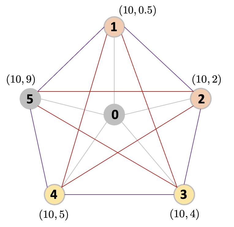
Figure 1: Example graph. Weights of grey/purple/red edges are $0.5/1/1.5$ respectively. Labels next to each vertex display $(p_{i},\bar{p}^{k}_{i})$ for all $k$.

Consider the complete graph with $6$ nodes in Figure 1, where node $0$ is the depot. Assume that there are two carriers $a$ and $b$, and that for all $k\in\{k_{1},k_{2}\}$:

• $c_{0j}^{k}=0.5$ for all $j\in V$, $c_{12}^{k}=c_{23}^{k}=c_{34}^{k}=c_{45}^{k}=c_{51}^{k}=1$, $c_{13}^{k}=c_{14}^{k}=c_{24}^{k}=c_{25}^{k}=c_{35}^{k}=1.5$, and $c_{ij}^{k}=c_{ji}^{k}$ for all $(i,j)\in A$;

• $b^{k}=2$;

• $(p_{1},\bar{p}_{1}^{k})=(10,0.5)$, $(p_{2},\bar{p}_{2}^{k})=(10,2)$, $(p_{3},\bar{p}_{3}^{k})=(10,4)$, $(p_{4},\bar{p}_{4}^{k})=(10,5)$, $(p_{5},\bar{p}_{5}^{k})=(10,9)$.

Let us suppose that the platform maximizes its own profit, while imposing that the profit of the carriers is larger than a certain threshold, e.g., their willingness to accept (WTA), and assuming that this suffices to have $P_{k}=Q_{k}$ (each carrier serves what is assigned to her). Assume also that the WTA value for both carriers is 0, i.e., both are willing to accept to serve in case the net profit is greater than 0. In this single-level setting, which we call the WTA-PTP, the leader would assign to carriers $k_{1}$ and $k_{2}$ items $1$, $2$, $3,$ and $4$ (two to each carrier, see the colors of the nodes in Figure 1 for an example), predicting a total profit of $28.5$. The platform would exclude item $5$ because it corresponds to the smallest margin of $1$. Let us now consider the BPFM as described above. The carrier who is assigned item $1$, together with any other item among $2$, $3,$ and $4$, would not deliver it, since serving only the other offered item ($2$, $3$, or $4$) would produce a higher profit than serving the assigned pair. Thus, the profit of the leader associated with their optimal WTA-PTP solution is $19$, while the optimal solution of the BPMF excludes item $1$ and includes item $5$, yielding a total profit of $20$. This example illustrates that it is crucial to integrate the optimal followers’ response inside of the optimization problem, as it is done with the BPMF. Approximating this optimal response, and replacing it with, e.g., WTA assumption leads to a suboptimal solution for the leader. Nevertheless, the value of WTA-PTP can be used to derive an upper bound on the net profit of the leader in the bilevel setting (with the WTA threshold of each carrier, set to zero).

This shows that the problem we study is bilevel in nature and that, to avoid misprediction of the true profit of the leader, we need to anticipate the optimal response of the carriers.

3.1 Mathematical formulations of the Bilevel PTP with Fixed Margins

In this section, we introduce a formulation for the BPFM with a limit on the number of packages. We recall that in the BPFM the leader does not decide on the compensations to be paid to the carriers, i.e., $\bar{p}_{i}^{k}$ is fixed and given a-priori.

To model the leader’s decision on the proposal to each carrier, we use binary decision variables $x^{k}_{i}$, $i\in V$, $k\in K$, which take the value 1, iff the platform assigns customer $i$ to carrier $k$, i.e., if $i\in P_{k}$. In addition, we define the lower-level binary variable $y^{k}_{i}$ for each $i\in V_{0}$ and $k\in K$, to model the acceptance decision of the carriers. $y^{k}_{i}$ is 1, iff carrier $k$ accepts to serve customer $i$, i.e., $i\in Q_{k}$; in particular, $y^{k}_{0}$ is equal to 1 in case carrier $k$ accepts to make at least one delivery. Finally, we consider the set of lower-level binary variables $z^{k}_{ij}$ for all $(i,j)\in A$ and $k\in K$ to model the routing decisions of the carriers. In particular, $z^{k}_{ij}=1$ iff arc $\left(i,j\right)\in A$ is traversed by carrier $k$.

Then, the BPFM formulation is as follows:

$$\max\limits_{x,y} \quad\sum_{i\in V}\sum_{k\in K}\left(p_{i}-\bar{p}^{k}_{i}\right)y^{k}_{i}$$ (1a)

s.t. $$\quad\sum_{k\in K}x^{k}_{i}\leq 1\qquad \forall\;i\in V$$ (1b)

$$\quad\sum_{i\in V}x^{k}_{i}\leq b^{k} \forall\;k\in K$$ (1c)

$$\quad y^{k}\in S^{k}_{\varphi}(x^{k}) \forall\;k\in K$$ (1d)

$$\quad x^{k}\in\{0,1\}^{n} \forall\;k\in K,$$ (1e)

where $S^{k}_{\varphi}(x^{k})$ is the set of optimal solutions of the $k$-th follower problem, which, for a given $\tilde{x}^{k}$, is formulated as:

$$\varphi^{k}(\tilde{x}^{k})=\quad\max\limits_{y,z} \quad\sum_{i\in V}\bar{p}^{k}_{i}y^{k}_{i}-\sum_{(i,j)\in A}c^{k}_{ij}z^{k}_{ij}$$ (2a)

s.t. $$\quad y^{k}_{i}\leq\tilde{x}^{k}_{i} \forall\;i\in V$$ (2b)

$$\quad(y^{k},z^{k})\text{ is a route}$$ (2c)

$$\quad y^{k}\in\{0,1\}^{n+1},z^{k}\in\{0,1\}^{|A|}.$$ (2d)

Constraints (1b) state that each item is offered to at most one carrier. Constraints (1c) impose that carrier $k$ should be offered to serve at most $b^{k}$ items. Constraints (1d) ensure that the solution $y^{k}$ returned by the $k$-th follower is an optimal response with respect to the set of items offered to her by the leader. The objective function (2a) of follower $k$ is the difference between the sum of the delivered items’ compensations and the total travel cost (length of the route that visits all customers accepted by the carrier). Constraints (2b) link the decisions of the leader with the ones of the follower, and establish that an item $i$ can be delivered by carrier $k$ only if it is offered to her. Finally, constraint (2c) states that $z^{k}$ is the incidence vector of a route that visits the depot and all customers $i$ such that $y^{k}_{i}=1$. More in detail, constraint (2c) is given by:

$$\sum\limits_{(i,j)\in\delta^{+}(i)}z_{ij}^{k}\;=\; y_{i}^{k} \quad\forall\;i\in V$$ (3a)

$$\sum\limits_{(i,j)\in\delta^{-}(i)}z_{ji}^{k}\;=\; y_{i}^{k} \quad\forall\;i\in V$$ (3b)

$$\sum\limits_{i\in S,j\in S}z_{ij}^{k}\;\leq\; \sum_{i\in S}y_{i}-y_{h} \quad\forall\;S\subseteq V,|S|\geq 2,h\in S.$$ (3c)

The first two sets of equalities (3a)–(3b) impose that one arc enters and leaves each visited vertex. The last set of exponentially many inequalities (3c) ensures subtour elimination and connection to the depot.

3.1.1 A Single-Level Reformulation

To derive a single-level reformulation of the BPFM formulation (1), we follow the value function reformulation approach presented in Appendix A. The corresponding formulation reads:

$$\max\limits_{x,y,z} \quad\sum_{i\in V}\sum_{k\in K}\left(p_{i}-\bar{p}^{k}_{i}\right)y^{k}_{i}$$ (4a)

s.t. $$\quad\sum_{k\in K}x^{k}_{i}\leq 1\qquad \forall\;i\in V$$ (4b)

$$\quad\sum_{i\in V}x^{k}_{i}\leq b^{k} \forall\;k\in K$$ (4c)

$$\quad\sum_{i\in V}\bar{p}^{k}_{i}y^{k}_{i}-\sum_{(i,j)\in A}c^{k}_{ij}z^{k}_{ij}\geq\varphi^{k}(x^{k}) \forall\;k\in K$$ (4d)

$$\quad y^{k}_{i}\leq x^{k}_{i} \forall\;i\in V,k\in K$$ (4e)

$$\quad(y^{k},z^{k})\text{ is a route} \forall\;k\in K$$ (4f)

$$\quad x^{k}{\in\{0,1\}^{n}},y^{k}\in\{0,1\}^{n+1},z^{k}\in\{0,1\}^{|A|} \forall\;k\in K.$$ (4g)

The difficulty of solving formulation (4) lies in the value-function constraints (4d): the function $\varphi^{k}(x^{k})$ is non-convex and non-continuous. Thus, in order to derive a single-level MIP formulation of the problem, we further analyze this function, which we try to convexify. Under the assumption that arc weights $c^{k}_{ij}$ satisfy the triangle inequality (in order to ensure that $z^{k}_{ij}=1$ implies $y^{k}_{i}=y^{k}_{j}=1$ for all $k$), we derive the following result.

Proposition 1.

For any $k\in K$, given a vector $\tilde{x}^{k}\in\{0,1\}^{n}$ satisfying constraints (4b)–(4c), there always exists an optimal solution of the following problem, which is also optimal for $\varphi^{k}(\tilde{x}^{k})$:

$$\bar{\varphi}^{k}(\tilde{x}^{k})=\quad\max\limits_{y,z} \quad\sum_{i\in V}\bar{p}^{k}_{i}y^{k}_{i}\tilde{x}^{k}_{i}-\sum_{(i,j)\in A}c^{k}_{ij}z^{k}_{ij}$$ (5a)

s.t. $$\quad(y^{k},z^{k})\text{ is a route}$$ (5b)

$$\quad y^{k}\in\{0,1\}^{n+1},z^{k}\in\{0,1\}^{|A|}.$$ (5c)

Proof.

Let $\tilde{x}^{k}\in\{0,1\}^{n}$ be a vector satisfying constraints (4b)–(4c). Let us consider a given $k\in K$ and let $P_{k}\subseteq V$ be the subset of vertices associated with $\tilde{x}^{k}$, i.e. $P_{k}=\{i\in V:\tilde{x}^{k}_{i}=1\}$. Being $S_{\bar{\varphi}}^{k}(\tilde{x}^{k})$ the set of optimal solutions of problem $\varphi^{k}(\tilde{x}^{k})$, we want to prove that there exists $(\hat{y}^{k},\hat{z}^{k})\in S_{\bar{\varphi}}^{k}(\tilde{x}^{k})$ s.t. (i) its objective function value is $\sum\limits_{i\in P_{k}}\bar{p}^{k}_{i}\hat{y}^{k}_{i}-\sum\limits_{(i,j)\in A}c^{k}_{ij}\hat{z}^{k}_{ij}$, and (ii) $\hat{y}^{k}_{i}=0$ for all $i\in V\setminus P_{k},$ despite the relaxation of constraints (2b) in formulation (5). Indeed, if an $i^{\prime}\in V\setminus P_{k}$ exists s.t. $\hat{y}^{k}_{i^{\prime}}=1$, then the compensation collected from $i^{\prime}$ would be 0 as $\tilde{x}^{k}_{i^{\prime}}=0$. Also, because of the triangle inequality, going directly from the predecessor to the successor of $i^{\prime}$ in the optimal solution is cheaper (or at most has the same cost) than going through $i^{\prime}$. Thus, either the solution visiting $i^{\prime}$ is not optimal, or there exists a solution that does not visit $i^{\prime}$ with the same value of the objective function. This procedure can be iterated over all vertices in $V\setminus P_{k}$. ∎

According to Proposition 1, the problem of follower $k$ could be solved by considering the entire graph $\cal{G}$ and multiplying the compensation associated with each customer $i\in V$ by the value $\tilde{x}_{i}^{k}$, representing the assignment made by the leader. In this way, in case $\tilde{x}_{i}^{k}=0$, customer $i$ would not be visited in the optimal solution of follower $k$.

Let $P^{k}_{ext}$ denote the set of all the extreme points $(y^{k},z^{k})$ of the convex hull of the follower’s feasible solutions space determined by constraints (5b)–(5c). It holds that:

$$\varphi^{k}(x^{k})=\max_{(\hat{y}^{k},\hat{z}^{k})\in P^{k}_{ext}}\left\{\sum_{i\in V}\bar{p}^{k}_{i}\hat{y}^{k}_{i}x^{k}_{i}-\sum_{(i,j)\in A}c^{k}_{ij}\hat{z}^{k}_{ij}\right\},$$

which is a convex function in $x^{k}$.

We notice that, in terms of routes $T\in\mathcal{T},$ problem (5) can be restated as:

$$\bar{\varphi}^{k}(\tilde{x}^{k})=\max\limits_{T\in\mathcal{T}}\left\{\sum_{i\in V(T)}\bar{p}_{i}^{k}\tilde{x}^{k}_{i}-C^{k}(T)\right\}.$$

In other words, constraints (4d) can be replaced by constraints

$$\sum_{i\in V}\bar{p}^{k}_{i}y^{k}_{i}-\sum_{(i,j)\in A}c^{k}_{ij}z^{k}_{ij}\geq\sum_{i\in V(T)}\bar{p}_{i}^{k}x^{k}_{i}-C^{k}(T)\qquad\forall\;T\in\mathcal{T},\;k\in K,$$ (6)

obtaining the following single-level reformulation of problem (4):

$$\max\limits_{x,y,z} \quad\sum_{i\in V}\sum_{k\in K}\left(p_{i}-\bar{p}^{k}_{i}\right)y^{k}_{i}$$ (7a)

s.t. $$\quad\eqref{eq:routing_single-partition1}\text{--}\eqref{eq:routing_single-budget1}$$ (7b)

$$\quad\sum_{i\in V}\bar{p}^{k}_{i}y^{k}_{i}-\sum_{(i,j)\in A}c^{k}_{ij}z^{k}_{ij}\geq\sum_{i\in V(T)}\bar{p}_{i}^{k}x^{k}_{i}-C^{k}(T) \forall\;T\in\mathcal{T},\;k\in K$$ (7c)

$$\quad y^{k}_{i}\leq x^{k}_{i} \forall\;i\in V,k\in K$$ (7d)

$$\quad(y^{k},z^{k})\text{ is a route} \forall\;k\in K$$ (7e)

$$\quad x^{k}\in\{0,1\}^{n},y^{k}\in\{0,1\}^{n+1},z^{k}\in\{0,1\}^{|A|} \forall\;k\in K,$$ (7f)

to which we will refer in the rest of the paper when considering the BPFM.

3.2 Mathematical formulations of the Bilevel PTP with Margin Decisions

In this section, we turn our attention to the BPMD and present two different formulations for this problem. As already discussed, in this problem we assume that, in addition to assignment decisions, the leader decides also the margin $m\in M$ to gain from each item $i$ delivered by carrier $k$.

Let $m_{\text{min}}$ and $m_{\text{max}}$ be the minimum and maximum margin, respectively. In order to model the leader’s choice among the different values of margins $m\in M$ we have considered the following two alternative options:

• We define a new upper-level binary variable for each carrier, margin, and item, $X_{mi}^{k}$, which takes value $1$ iff $i\in P_{k}$ and the selected margin is $m$ for item $i$, and $0$ otherwise. Since $\sum\limits_{m\in M}X_{mi}^{k}=x_{i}^{k}$ for all $i\in V$ and $k\in K$, we can discard the variables $x$. However, we still use the decision variables $y$ as defined for the BPFM.

• We define also the lower-level binary disaggregated variable $Y_{mi}^{k}$, which substitutes the previous decision variable $y^{k}_{i}$, and takes value $1$ iff carrier $k$ accepts to serve customer $i$ (i.e., $i\in Q_{k}$) with margin level $m$.

In both cases, we model the routing decisions with the same binary variables $z$ as defined for the BPFM. The decision variables of alternative (i) lead to what we call the aggregated formulation, in contrast to alternative (ii) which leads to a disaggregated formulation. We prove in Subsection 3.3 that the two formulations provide the same bounds.

Before presenting the formulations we observe that if the selected margin is $m$, the corresponding net profit for the leader will be $p_{mi}y_{i}^{k}$, where $p_{mi}=m\cdot p_{i}$. Furthermore, in this context, we denote by $\bar{p}_{mi}=p_{i}-p_{mi}$ the compensation paid to follower $k$ when the selected margin is $m$.

3.2.1 Aggregated formulation.

Using the decision variables of alternative (i), the upper-level variable $x_{i}^{k}$ can be replaced by $\sum\limits_{m\in M}X_{mi}^{k}.$ Furthermore, the upper-level objective function, representing the net profit of the leader to be maximized, reads as

$$\sum_{k\in K}\sum_{i\in V}\sum_{m\in M}p_{mi}X_{mi}^{k}y_{i}^{k}.$$

We can linearize this function by using Fortet’s inequalities (Fortet, 1960), i.e., a special case of the McCormick inequalities for products of binary variables. Such inequalities define the convex envelopes of the bilinear terms $X^{k}_{mi}y^{k}_{i}$. In order to do this, we have to introduce additional binary variables $w_{mi}^{k}$ defined as $X_{mi}^{k}y^{k}_{i}$, and insert the Fortet’s inequalities (8d)–(8f) in the upper-level problem formulation obtaining the following bilevel problem:

$$\max\limits_{X,y,w} \quad\sum_{k\in K}\sum_{i\in V}\sum_{m\in M}p_{mi}w_{mi}^{k}$$ (8a)

s.t. $$\quad\sum_{k\in K}\sum_{m\in M}X^{k}_{mi}\leq 1\qquad \forall\;i\in V$$ (8b)

$$\quad\sum_{i\in V}\sum_{m\in M}X^{k}_{mi}\leq b^{k} \forall\;k\in K$$ (8c)

$$\quad X_{mi}^{k}+y^{k}_{i}\leq w_{mi}^{k}+1 \forall\;m\in M,i\in V,k\in K$$ (8d)

$$\quad w_{mi}^{k}\leq X_{mi}^{k} \forall\;m\in M,i\in V,k\in K$$ (8e)

$$\quad w_{mi}^{k}\leq y^{k}_{i} \forall\;m\in M,i\in V,k\in K$$ (8f)

$$\quad y^{k}\in S^{k}_{\Phi}(X^{k}) \forall\;k\in K$$ (8g)

$$\quad y^{k},X_{m}^{k},w^{k}\in\{0,1\}^{n+1} \forall\;m\in M,k\in K,$$ (8h)

where $S^{k}_{\Phi}(X^{k})$ is the set of optimal solutions of the $k$-th follower problem, which, for a given $\tilde{X}^{k}$, reads:

$$\Phi^{k}(\tilde{X}^{k})=\;\max\limits_{y,z} \;\sum_{i\in V}\sum_{m\in M}\bar{p}_{mi}\tilde{X}_{mi}^{k}y^{k}_{i}-\sum_{(i,j)\in A}c^{k}_{ij}z^{k}_{ij}$$ (9a)

s.t. $$\quad y^{k}_{i}\leq\sum_{m\in M}\tilde{X}^{k}_{mi} \forall\;i\in V$$ (9b)

$$\quad(y^{k},z^{k})\text{ is a route}$$ (9c)

$$\quad y^{k}\in\{0,1\}^{n+1},z^{k}\in\{0,1\}^{|A|}.$$ (9d)

We note that, if $\sum\limits_{m\in M}X_{mi}^{k}=0,$ then $X_{mi}^{k}=0$ for all $m$, and hence $y_{i}^{k}$ will be $0$ (from constraints (9b)), so the upper-level objective function, as well as the first term of the lower-level objective function, will also be 0. Thus, we can replace constraints (8d) by:

$$y^{k}_{i}\leq w_{mi}^{k}+\sum_{u\in M:u\neq m}X_{ui}^{k}\quad\quad\forall\;m\in M,i\in V,k\in K.$$ (10a)

Furthermore, to strengthen the Linear Programming (LP) relaxation of the problem, we add the following constraint, implicitly satisfied for binary solutions, but not necessarily for LP solutions:

$$y^{k}_{i}=\sum_{m\in M}w_{mi}^{k}\quad\quad\forall\;i\in V,k\in K.$$ (10b)

A single-level reformulation of the proposed bilevel problem may be obtained using the value function reformulation. Similarly to what we did in Section 3.1, under the assumption that the parameters $c^{k}_{ij}$ satisfy the triangle inequality, we have the following result.

Proposition 2.

For any $k\in K$, given a vector $\tilde{X}^{k}\in\{0,1\}^{n+1}$ satisfying constraints (8b)–(8e), there always exists an optimal solution of the following problem, which is also optimal for $\Phi^{k}(\tilde{X}^{k})$:

$$\bar{\Phi}^{k}(\tilde{X}^{k})=\quad\max\limits_{T\in\mathcal{T}}\left\{\sum_{i\in V(T)}\sum_{m\in M}\bar{p}_{mi}\tilde{X}_{mi}^{k}-C^{k}(T)\right\}.$$ (11)

Proof.

Problem (11) is obtained from (9) by relaxing constraints (9b), i.e., $y_{i}\leq\sum\limits_{m\in M}\tilde{X}^{k}_{mi}$. When, for a given $i^{\prime}\in V$, $\sum\limits_{m\in M}\tilde{X}^{k}_{mi^{\prime}}=1$, this constraint is implicitly satisfied, being $y$ at most 1. Thus, being $S_{\bar{\Phi}}^{k}(\tilde{X}^{k})$ the set of optimal solutions of problem ${\bar{\Phi}}^{k}(\tilde{X}^{k})$, we want to prove that, if, for a given $i^{\prime}$, $\sum\limits_{m\in M}\tilde{X}^{k}_{mi^{\prime}}=0$ there exists $(\hat{y}^{k},\hat{z}^{k})\in S_{\bar{\Phi}}^{k}(\tilde{X}^{k})$ such that $\hat{y}^{k}_{i^{\prime}}=0$. Assume that $\hat{y}^{k}_{i^{\prime}}=1$, then the compensation collected from $i^{\prime}$ would be 0 as $\tilde{X}^{k}_{mi^{\prime}}=0$ for all $m$. Also, because of the triangle inequality, going directly from the predecessor to the successor of $i^{\prime}$ in the optimal solution is cheaper (or at most has the same cost) than going through $i^{\prime}$. Thus, either the solution visiting $i^{\prime}$ is not optimal, or there exists a solution that does not visit $i^{\prime}$ with the same value of the objective function. ∎

Following the same approach as in Proposition 1, we have the following single-level reformulation:

$$\max\limits_{X,y,w,z} \quad\sum_{k\in K}\sum_{i\in V}\sum_{m\in M}p_{mi}w_{mi}^{k}$$ (12a)

s.t. $$\quad\eqref{eq:pricing1-partition}\text{--}\eqref{eq:pricing1-budget},\eqref{eq:pricing1-mc1bis}\text{--}\eqref{eq:pricing1-yw},\eqref{eq:pricing1-mc2}\text{--}\eqref{eq:pricing1-mc3}$$

$$\quad y_{i}^{k}\leq\sum_{m\in M}X_{mi}^{k} \forall\;i\in V,k\in K$$ (12b)

$$\quad(y^{k},z^{k})\text{ is a route} \forall\;k\in K$$ (12c)

$$\sum_{i\in V}\sum_{m\in M}\bar{p}_{mi}w_{mi}^{k}-\sum_{(i,j)\in A}c^{k}_{ij}z^{k}_{ij}\geq\sum_{i\in V(T)}\sum_{m\in M}\bar{p}_{mi}X_{mi}^{k}-C^{k}(T) \forall\;T\in\mathcal{T},k\in K$$ (12d)

$$\quad y^{k},X_{m}^{k},w_{m}^{k}\in\{0,1\}^{n+1},z^{k}\in\{0,1\}^{|A|} \forall\;m\in M,k\in K,$$ (12e)

where constraints (12d) replace the value function constraints

$$\sum_{i\in V}\sum_{m\in M}\bar{p}_{mi}w_{mi}^{k}-\sum_{(i,j)\in A}c^{k}_{ij}z^{k}_{ij}\geq\Phi^{k}(X^{k})\quad\forall\;k\in K.$$

3.2.2 Disaggregated formulation.

Using the disaggregated decision variable $Y_{mi}^{k}$ of alternative (ii), we obtain the following formulation:

$$\max\limits_{X,Y} \quad\sum_{k\in K}\sum_{i\in V}\sum_{m\in M}\left(p_{mi}Y^{k}_{mi}\right)$$ (13a)

s.t. $$\quad\sum_{k\in K}\sum_{m\in M}X^{k}_{mi}\leq 1\qquad \forall\;i\in V$$ (13b)

$$\quad\sum_{i\in V}\sum_{m\in M}X^{k}_{mi}\leq b^{k} \forall\;k\in K$$ (13c)

$$\quad Y^{k}\in S^{k}_{\Psi}(X^{k}) \forall\;k\in K$$ (13d)

$$\quad X_{m}^{k}\in\{0,1\}^{n} \forall\;m\in M,k\in K,$$ (13e)

where $S^{k}_{\Psi}(X^{k})$ is the set of optimal solutions of the $k$-th follower problem, which, for a given $(\tilde{X}^{k})$, is formulated as:

$$\Psi^{k}(\tilde{X}^{k})=\;\max\limits_{Y,z} \;\sum_{i\in V}\sum_{m\in M}\bar{p}_{mi}Y^{k}_{mi}-\sum_{(i,j)\in A}c^{k}_{ij}z^{k}_{ij}$$ (14a)

s.t. $$\quad Y^{k}_{mi}\leq\tilde{X}^{k}_{mi} \forall\;i\in V,m\in M$$ (14b)

$$\quad(\sum_{m\in M}Y^{k}_{m},z^{k})\text{ is a route}$$ (14c)

$$\quad Y_{m}^{k}\in\{0,1\}^{n+1},z^{k}\in\{0,1\}^{|A|} \forall\;m\in M.$$ (14d)

In this second formulation, we do not need to use Fortet’s inequalities, since, thanks to the disaggregated variable $Y_{mi}^{k}$, there is no bilinear product to linearize. In this case, a route $T\in\mathcal{T}$ corresponds to the pair $(\sum\limits_{m\in M}Y^{k}_{mi},z^{k})$. As before, under the assumption that the $c^{k}_{ij}$ satisfy the triangle inequality (in order to ensure that $z^{k}_{ij}=1$ implies $Y^{k}_{i}=Y^{k}_{j}=1$ for all $k$), we have the following result.

Proposition 3.

For any $k\in K$, given a vector $\tilde{X}^{k}\in\{0,1\}^{n}$ satisfying constraints (13b)–(13c), there always exists an optimal solution of the following problem, which is also optimal for $\Psi^{k}(\tilde{X}^{k})$:

$$\bar{\Psi}^{k}(\tilde{X}^{k})=\;\max\limits_{T\in\mathcal{T}}\left\{\sum_{i\in V(T)}\sum_{m\in M}\bar{p}_{mi}\tilde{X}^{k}_{mi}-C^{k}(T)\right\}.$$ (15a)

Note that the proof of Proposition 3 is similar to the one of Proposition 1, so it is omitted.

The single-level reformulation is then:

$$\max\limits_{X,Y,z} \quad\sum_{k\in K}\sum_{i\in V}\sum_{m\in M}p_{mi}Y^{k}_{mi}$$ (16a)

s.t. $$\quad\eqref{eq:pricing2-partition}\text{--}\eqref{eq:pricing2-budget}$$ (16b)

$$\quad Y^{k}_{mi}\leq X^{k}_{mi} \forall\;i\in V,m\in M,k\in K$$ (16c)

$$\quad(\sum_{m\in M}Y^{k}_{m},z^{k})\text{ is a route} \forall\;k\in K$$ (16d)

$$\quad\sum_{i\in V}\sum_{m\in M}\bar{p}_{mi}Y^{k}_{mi}-\sum_{(i,j)\in A}c^{k}_{ij}z^{k}_{ij}\geq$$

$$\quad\quad\quad\quad\quad\quad\quad\quad\quad\sum_{i\in V(T)}\sum_{m\in M}\bar{p}_{mi}\tilde{X}^{k}_{mi}-C^{k}(T) \forall\;T\in\mathcal{T},k\in K$$ (16e)

$$\quad X_{m}^{k}\in\{0,1\}^{n},Y_{m}^{k}\in\{0,1\}^{n+1},z^{k}\in\{0,1\}^{|A|} \forall\;m\in M,k\in K,$$ (16f)

were constraints (16e) reformulate, according to Proposition 3, the value function constraints

$$\sum_{i\in V}\sum_{m\in M}\bar{p}_{mi}Y^{k}_{mi}-\sum_{(i,j)\in A}c^{k}_{ij}z^{k}_{ij}\geq\Psi^{k}(X^{k})\quad\forall\;k\in K.$$

3.3 Comparing the two BPMD formulations

In this section, we compare the two BPMD formulations, $\mathsf{{\color[rgb]{0,0.6,0}BPMD}}$ and $\mathsf{{\color[rgb]{0,0.6,0}BPMD_{d}}}$, in terms of the value of their linear relaxations. In the following theorem, we prove that the aggregated formulation $\mathsf{{\color[rgb]{0,0.6,0}BPMD}}$ is as strong as formulation $\mathsf{{\color[rgb]{0,0.6,0}BPMD_{d}}}$ (i.e., its linear relaxation provides equivalent upper bounds). Let us define $v_{LP}(\mathsf{{\color[rgb]{0,0.6,0}BPMD}})$ and $v_{LP}(\mathsf{{\color[rgb]{0,0.6,0}BPMD_{d}}})$ as the optimal values of the LP relaxation of $\mathsf{{\color[rgb]{0,0.6,0}BPMD}}$ and $\mathsf{{\color[rgb]{0,0.6,0}BPMD_{d}}}$, respectively.

Theorem 1.

Any LP feasible solution $(\tilde{X},\tilde{y},\tilde{w},\tilde{z})$ of the model $\mathsf{{\color[rgb]{0,0.6,0}BPMD}}$ can be translated into a LP feasible solution $(\tilde{X},\tilde{Y},\tilde{z})$ of the model $\mathsf{{\color[rgb]{0,0.6,0}BPMD_{d}}}$ by imposing that, for all $i\in V,m\in M,k\in K$:

$$\tilde{Y}_{mi}^{k}=\tilde{w}^{k}_{mi},\quad(\star)$$

and vice versa. Hence $v_{LP}(\mathsf{{\color[rgb]{0,0.6,0}BPMD}})=v_{LP}(\mathsf{{\color[rgb]{0,0.6,0}BPMD_{d}}})$.

Proof.

Let us start by proving that $v_{LP}(\mathsf{{\color[rgb]{0,0.6,0}BPMD}})\leq v_{LP}(\mathsf{{\color[rgb]{0,0.6,0}BPMD_{d}}})$, i.e., that any LP solution $(\tilde{X},\tilde{y},\tilde{w},\tilde{z})$ of $\mathsf{{\color[rgb]{0,0.6,0}BPMD}}$ is also feasible in $\mathsf{{\color[rgb]{0,0.6,0}BPMD_{d}}}$, when imposing Eq. $(\star)$. Indeed, constraints (13b) and (13c) are constraints (8b) and (8c), respectively. Constraints (16c) correspond to (8e). Constraints (16e) is equivalent to constraints (12d). Finally, constraints (16d) correspond to (12c) combined with constraints (10b). Hence the inequality $v_{LP}(\mathsf{{\color[rgb]{0,0.6,0}BPMD}})\leq v_{LP}(\mathsf{{\color[rgb]{0,0.6,0}BPMD_{d}}})$ holds. Let us now consider an LP solution $(\tilde{X},\tilde{Y},\tilde{z})$ of $\mathsf{{\color[rgb]{0,0.6,0}BPMD_{d}}}$. We need to show that it is LP feasible also for $\mathsf{{\color[rgb]{0,0.6,0}BPMD}}$ if Eq. $(\star)$ is imposed. Indeed, as already said, constraints (8b), (8c), (8e) and (12d) correspond to (13b), (13c), (16c) and (16e), respectively. For the remaining constraints, in model $\mathsf{{\color[rgb]{0,0.6,0}BPMD_{d}}}$, we can replace variable $y_{i}^{k}$ by $\sum\limits_{m\in M}w_{mi}^{k}$ by constraint (10b). Therefore:

• Constraints (8f) reads $w_{mi}^{k}\leq\sum\limits_{u\in M}w_{ui}^{k}$. They are satisfied by $(\tilde{X},\tilde{Y},\tilde{z})$, because $\tilde{Y}_{mi}^{k}\geq 0\;\forall\;m\in M,i\in V,k\in K$, and thus $\tilde{Y}_{mi}^{k}\leq\sum\limits_{u\in M}\tilde{Y}_{ui}^{k}$.

• Constraints (10a) read $\sum\limits_{u\in M}w_{ui}^{k}\leq w_{mi}^{k}+\sum\limits_{u\in M:u\neq m}X_{ui}^{k}$. They are satisfied by $(\tilde{X},\tilde{Y},\tilde{z})$ because for all $m\in M,i\in V,k\in K$:

  $$\sum_{u\in M}\tilde{Y}_{ui}^{k}\leq\tilde{Y}_{mi}^{k}+\sum_{u\in M:u\neq m}\tilde{X}_{ui}^{k}\iff\sum_{u\in M:u\neq m}\tilde{Y}_{ui}^{k}\leq\sum_{u\in M:u\neq m}\tilde{X}_{ui}^{k}$$

  hold since $\tilde{Y}_{ui}^{k},\tilde{X}_{ui}^{k}\geq 0$ and $\tilde{Y}_{ui}^{k}\leq\tilde{X}_{ui}^{k}$ for all $u\in M,i\in V,k\in K$ from (16c).

• Constraints (12b) read $\sum\limits_{m\in M}w_{mi}^{k}\leq\sum\limits_{m\in M}X_{mi}^{k}$. They are satisfied by $(\tilde{X},\tilde{Y},\tilde{z})$ because $\sum\limits_{m\in M}\tilde{Y}_{mi}^{k}\leq\sum\limits_{m\in M}\tilde{X}_{mi}^{k}$ holds since $\tilde{Y}_{mi}^{k},\tilde{X}_{mi}^{k}\geq 0$ and $\tilde{Y}_{mi}^{k}\leq\tilde{X}_{mi}^{k}$ for all $m\in M,i\in V,k\in K$ from (16c).

• Constraints (12c) read “$(\sum\limits_{m\in M}w_{m}^{k},z^{k})$ is a route” for all $k\in K$, which correspond to constraints (16d).

Hence, also inequality $v_{LP}(\mathsf{{\color[rgb]{0,0.6,0}BPMD}})\geq v_{LP}(\mathsf{{\color[rgb]{0,0.6,0}BPMD_{d}}})$ holds. Consequently, we have that $v_{LP}(\mathsf{{\color[rgb]{0,0.6,0}BPMD}})=v_{LP}(\mathsf{{\color[rgb]{0,0.6,0}BPMD_{d}}}).$ ∎

3.4 Projecting out the $z$ variables

In this section, we present new formulations derived from projecting out the $z$ variables in both value-function reformulations presented above. We introduce the new continuous variables $\theta^{k}$, for each $k\in K$, which represent the cost of the route followed by carrier $k$. In this case, problem $(\mathsf{{\color[rgb]{0,0.6,0}BPFM}})$ becomes

$$\max\limits_{x,y,\theta} \quad\sum_{i\in V}\sum_{k\in K}\left(p_{i}-\bar{p}^{k}_{i}\right)y^{k}_{i}$$ (17a)

s.t. $$\quad\sum_{k\in K}x^{k}_{i}\leq 1 \forall\;i\in V$$ (17b)

$$\quad\sum_{i\in V}x^{k}_{i}\leq b^{k} \forall\;k\in K$$ (17c)

$$\quad\sum_{i\in V}\bar{p}^{k}_{i}y^{k}_{i}-\theta^{k}\geq\varphi^{k}(x^{k}) \forall\;k\in K$$ (17d)

$$\quad\theta^{k}\geq c_{\mathsf{TSP}}(y^{k}) \forall\;k\in K$$ (17e)

$$\quad y^{k}_{i}\leq x^{k}_{i} \forall\;i\in V,k\in K$$ (17f)

$$\quad x^{k}\in\{0,1\}^{n},y^{k}\in\{0,1\}^{n+1},\theta^{k}\in\mathbb{R} \forall\;k\in K$$ (17g)

where $c_{\mathsf{TSP}}(y^{k})$ is the cost of the optimal route associated with vector $y_{k}$, and $\varphi^{k}(x^{k})$ is the optimal solution value of the $k$-th follower problem, which, for a given $(\tilde{x}^{k})$ is formulated as in (2).

According to Proposition 1, constraints (17d) can be replaced by:

$$\sum_{i\in V}\bar{p}_{i}^{k}y_{i}^{k}-\theta^{k}\geq\sum_{i\in V(T)}\bar{p}_{i}^{k}x^{k}_{i}-C^{k}(T)\quad\forall\;T\in\mathcal{T},k\in K,$$ (18a)

whereas constraints (17e) can be replaced by the cuts:

$$\theta^{k}\geq c_{\mathsf{TSP}}(V(T))\left[\sum_{i\in V(T)}y^{k}_{i}-|V(T)|+1\right]\quad\forall\;T\in\mathcal{T},k\in K.$$ (18b)

In the same way, when introducing the new real variable $\theta^{k}$, constraints (12c) and (12d) in $(\mathsf{{\color[rgb]{0,0.6,0}BPMD}})$ can be replaced by (18b) and:

$$\sum_{i\in V}\sum_{m\in M}\bar{p}_{mi}w_{mi}^{k}-\theta^{k}\geq\sum_{i\in V(T)}\sum_{m\in M}\bar{p}_{mi}X_{mi}^{k}-C^{k}(T) \quad\forall\;T\in\mathcal{T},k\in K$$ (19)

respectively, obtaining a new single-level formulation that we call $(\mathsf{{\color[rgb]{0,0.6,0}BPMD\text{-}z}})$.

Concerning problem (16), an equivalent single-level formulation, which we call $(\mathsf{{\color[rgb]{0,0.6,0}BPMD_{d}\text{-}z}})$, can be obtained by projecting out the $z$ variable and introducing the new variables $\theta^{k}$, replacing constraints (16d) and (16e) in $(\mathsf{{\color[rgb]{0,0.6,0}BPMD_{d}}})$ by:

$$\theta^{k}\geq c_{\mathsf{TSP}}(V(T))\left[\sum_{i\in V(T)}\sum_{m\in M}Y^{k}_{mi}-|V(T)|+1\right] \forall\;T\in\mathcal{T},k\in K$$ (20a)

$$\sum_{i\in V}\sum_{m\in M}\bar{p}_{mi}Y^{k}_{mi}-\theta^{k}\geq\sum_{i\in V(T)}\sum_{m\in M}\bar{p}_{mi}\tilde{X}^{k}_{mi}-C^{k}(T) \forall\;T\in\mathcal{T},k\in K.$$ (20b)

We refer to Appendix B for the complete formulations $(\mathsf{{\color[rgb]{0,0.6,0}BPMD\text{-}z}})$ and $(\mathsf{{\color[rgb]{0,0.6,0}BPMD_{d}\text{-}z}})$.

Additionally, we add to the formulation the following strengthening inequalities for all $k\in K$ in order to provide a non-trivial lower bound on the value of variables $\theta^{k}$:

$$\theta^{k}\geq\sum_{i\in V}d_{i}^{k}y_{i}^{k},$$ (21)

where $d_{i}^{k}=\max\{\min\limits_{j\in\delta^{-}(i)}c_{ji}^{k},\min\limits_{j\in\delta^{+}(i)}c_{ij}^{k}\}$. These inequalities state that the cost of the route associated with $y^{k}$ cannot be lower than the sum of the costs associated with the arcs of minimum cost incident to all the visited nodes.

3.5 Bounded route duration variant

In the setting considered above, each carrier cannot deliver more than $b^{k}$ packages (constraints (1c), (8c), (13c)). Another common practical setting is the one where the limitation is instead imposed on route duration, thus having a time limit $t_{max}^{k}$. To model this case, we remove the constraints on the maximum number of packages in the upper level and we add the following constraint:

$$\quad\sum\limits_{(i,j)\in A}c_{ij}^{k}z_{ij}^{k}\leq t_{max}^{k}$$ (22)

in each lower-level problem. The considerations on the bilevel nature of the problem also apply in this case.

The formulations presented in Section 3.4, where $z$ variables are projected out, have to include the following constraint:

$$\theta^{k}\leq t_{max}^{k}\quad\forall k\in K$$ (23)

in the single-level formulations, and constraint (22) in each lower level.

4 Solution approach

In this section, we present the solution approach we developed to solve the single-level formulations proposed in Section 3. We designed a branch-and-cut algorithm where value function constraints, as well as the no-good cuts related to the value of $\theta$ when projecting out $z$ variables, are separated dynamically as they are exponentially many. First, in Section 4.1, we discuss the separation procedures for the exponentially many constraints included in the models. Second, in Section 4.2, we present a heuristic algorithm, based on the solution of the BPFM, to generate a feasible solution used as a warm start for the exact approach for the BPMD.

4.1 Separation procedures

In this section, we describe the separation procedures we use to dynamically detect violated value function constraints in the single-level reformulations presented in Section 3. Indeed, we notice that these constraints are exponentially many and -hard to separate, as they require finding an optimal PTP solution, corresponding to an optimal follower response for a given assignment $x$ of the leader. Concerning the formulations with the $z$ variables, we notice that there is an exponential number of constraints of type (7c) in $(\mathsf{{\color[rgb]{0,0.6,0}BPFM}})$, and of type (12d) and (16e) in $(\mathsf{{\color[rgb]{0,0.6,0}BPMD}})$ and $(\mathsf{{\color[rgb]{0,0.6,0}BPMD_{d}}})$. In the formulations obtained by projecting out the $z$ variables, not only constraints (18a) in $(\mathsf{{\color[rgb]{0,0.6,0}BPFM\text{-}z}})$, (19) in $(\mathsf{{\color[rgb]{0,0.6,0}BPMD\text{-}z}})$, and (20b) in $(\mathsf{{\color[rgb]{0,0.6,0}BPMD_{d}\text{-}z}})$ are exponential in number, but also the no-good constraints (18b), and (20a), respectively.

We thus propose a separation procedure for these constraints, which we describe in the following referring to the problem with fixed margins, without loss of generality. We note that all constraints are separated on integer solutions only, in order to speed up the solution process.

Separation of constraints (7c)

When dealing with formulation $(\mathsf{{\color[rgb]{0,0.6,0}BPFM}})$, for any given solution $(\tilde{x},\tilde{y},\tilde{z})$ of the master problem, obtained by relaxing constraints (7c), we solve the profitable tour problem with $x=\tilde{x}$ for each $k$. Let $(\hat{y}^{k},\hat{z}^{k})$ be the optimal solution of the latter problem, with $\hat{T}^{k}$ and $\hat{\varphi}^{k}$ being the corresponding tour and value, respectively. If there exists a $k$ such that $\sum\limits_{i\in V}\bar{p}^{k}_{i}\tilde{y}^{k}_{i}-\sum\limits_{(i,j)\in A}c^{k}_{ij}\tilde{z}^{k}_{ij}<\hat{\varphi}^{k}$, then the following constraint

$$\sum_{i\in V}\bar{p}^{k}_{i}y^{k}_{i}-\sum_{(i,j)\in A}c^{k}_{ij}z^{k}_{ij}\geq\sum_{i\in V(\hat{T}^{k})}\bar{p}^{k}_{i}x^{k}_{i}-C^{k}(\hat{T}^{k})$$

is violated by the current solution of the master problem. Thus, we insert it into the master problem. Otherwise, the obtained solution is feasible (optimal if we are at the root node) for the original bilevel formulation.

Separation of constraints (18b)

When considering formulation $(\mathsf{{\color[rgb]{0,0.6,0}BPFM\text{-}z}})$, we have to separate constraints (18b) as well, which are also exponentially many. Thus, we first solve the master problem obtained by relaxing both (18a) and (18b), finding the solution $(\tilde{x},\tilde{y},\tilde{\theta})$, with the corresponding tour $\tilde{T}^{k}$ (with $c_{\mathsf{TSP}}(V(\hat{T}^{k}))$ the cost of the optimal route associated to $\tilde{T}^{k}$ nodes). Then, we solve the lower-level problems with $x=\tilde{x}$ for each $k$, obtaining the optimal solution $(\hat{y}^{k},\hat{z}^{k})$, the corresponding tour $\hat{T}^{k}$, and value $\hat{\varphi}^{k}$.

In the case in which there exists a $k$ such that $\tilde{\theta}^{k}<c_{\mathsf{TSP}}(V(\tilde{T}^{k}))$, we insert the following constraint:

$$\theta^{k}\geq c_{\mathsf{TSP}}(V(\tilde{T}^{k}))\left[\sum_{i\in V(\tilde{T}^{k})}y^{k}_{i}-|V(\tilde{T}^{k})|+1\right].$$ (24)

If instead, for all $k$, inequality

$$\tilde{\theta}^{k}\geq c_{\mathsf{TSP}}(V(\tilde{T}^{k})),$$ (25)

does hold, then we proceed with the separation of (18a) as we did for constraints (7c) above, i.e., if there exists a $k$ such that $\sum\limits_{i\in V}\bar{p}^{k}_{i}\tilde{y}^{k}_{i}-\tilde{\theta}^{k}<\hat{\varphi}^{k}$, then the we add the following constraint

$$\sum_{i\in V}\bar{p}^{k}_{i}y^{k}_{i}-\theta^{k}\geq\sum_{i\in V(\hat{T}^{k})}\bar{p}^{k}_{i}x^{k}_{i}-C^{k}(\hat{T}^{k})$$

to the master.

Separation of constraints (23)

When taking into account the maximum duration constraints (23) on variable $\theta^{k}$, we use the following separation procedure for each $k$:

• if $c_{\mathsf{TSP}}(V(\tilde{T}^{k}))\leq t_{max}^{k}$, we add cut (24);

• otherwise (i.e., if $c_{\mathsf{TSP}}(V(\tilde{T}^{k}))>t_{max}^{k}$), we cut off the solution $\tilde{y}^{k}$ because it is infeasible, adding the following no-good cut: $\sum\limits_{i\in V(\tilde{T}^{k})}y_{i}^{k}\leq|V(\tilde{T}^{k})|-1$.

4.2 Heuristic solution approach

In this section, we describe a heuristic procedure used to obtain a warm-start feasible solution for the branch-and-cut algorithm solving the BPMD. It consists of three phases, involving the solution of the BPFM.

First, the BPFM is solved by setting all the compensations to their highest values, i.e., $\bar{p}_{i}^{k}=(1-m_{\text{min}})p_{i}$ for all $i\in V,k\in K$. In this way, we obtain a first feasible solution to the BPMD. Note that, in case no package is assigned in this solution, then it means that no other solution exists in which any package is served. Indeed, this is the most rewarding compensation decision for the followers, and assigning no packages means that the compensations are still too low with respect to the routing costs.

In case the solution to the first step is nonempty, in the second step, BPMD is solved with all the variables, but the margin variables, fixed to the values returned by the first phase plus an additional constraint imposing that the profit of each carrier should be nonnegative. This corresponds to solving the following auxiliary problem, which is a multiple-choice knapsack solved independently for each follower:

$$\max_{X} \sum\limits_{k\in K}\sum\limits_{m\in M}\sum\limits_{i\in V(\hat{T})}p_{mi}X_{mi}^{k}$$ (26a)

s.t. $$\sum\limits_{m\in M}X_{mi}^{k}=\hat{x}^{k}_{i} \forall\;i\in V,k\in K$$ (26b)

$$\sum_{m\in M}\sum_{i\in V(\hat{T})}p_{mi}X_{mi}^{k}\leq\sum_{i\in V(\hat{T})}p_{i}-C(\hat{T}) \forall\;k\in K,$$ (26c)

where $\hat{x}$, and $\hat{T}$ come from the assignment and routing decisions made at the first step of the heuristic. The solution to the above problem determines which is the best margin decision for the leader, i.e., $\check{X}$, given the assignment of the items decided in the previous phase.

Finally, in the third step, the BPFM is solved again by fixing the margins according to the solution obtained in the second step, i.e., for each $i$ and $k$, we set $\bar{p}_{i}^{k}=p_{i}-\sum\limits_{m\in M}\check{X}_{mi}^{k}p_{mi}.$ The solution, together with $\check{X}$ found at the second step, is a feasible solution to the problem. Note that the third step is needed as, otherwise, the solution obtained from the second step might not be bilevel feasible, as it does not necessarily optimize the followers’ objective. The algorithm will then return the best solution in terms of the leader’s objective function between the one found in the first and the third step.

Depending on the presence of a budget constraint ((1c) or (13c)) or a route duration constraint ((22) or (23)) the problem to solve at each step changes. Indeed, when there is a constraint on the duration of the route, it is better to have a problem with the $z$ variable in the upper level, i.e., $(\mathsf{{\color[rgb]{0,0.6,0}BPFM}})$, since constraints (22) do not need to be separated. Instead, when there is no duration constraint, the problems without the $z$ variables $(\mathsf{{\color[rgb]{0,0.6,0}BPFM\text{-}z}})$, as expected, turn out to be faster after some preliminary experiments. The overall heuristic algorithm is described in Algorithm 1.

Input: Sets $V,A,K,M=\{m_{\text{min}},\dots,m_{\text{max}}\},$ and parameters $p_{i}$ for all $i\in V$, $c_{ij}^{k}$ for all $(i,j)\in A$, and $b^{k}$ (or $t_{max}^{k}$) for all $k\in K$.

Output: Feasible solution for BPMD.

1 Set $\bar{p}_{i}^{k}=(1-m_{\text{min}})p_{i}$ for all $i\in V,k\in K.$ Solve BPFM. Return the optimal solution in terms of assignment of the leader $\hat{x}$, and acceptance and routing decisions of the followers $\hat{T}$.

2 Solve problem (26). Return the optimal solution $\check{X}.$

3 Set $\bar{p}_{i}^{k}=p_{i}-\sum\limits_{m\in M}\check{X}_{mi}^{k}p_{mi}$ for all $i\in V,k\in K.$ Solve BPFM. Return the optimal solution $(\check{x},\check{T})$.

return the best solution between $(\check{x},\check{T})$, and $(\hat{x},\hat{T})$ in terms of leader’s objective function.

Algorithm 1 Heuristic algorithm for BPMD

5 Numerical Results

We tested the four different models developed in the previous sections on two sets of instances. For both classes, we considered the following sets of margins $M$: $\{0.2,0.5\},$ $\{0.5,0.9\},$ $\{0.2,0.5,0.8\},$ and $\{0.5,0.7,0.9\}.$ We restricted our tests to two or three margins as one might reasonably assume that, in practical settings, the choice may be among low and high margin or low, medium, and high margin. The value of the margins is selected after some preliminary experiments aimed at identifying values that generate different solution structures (as shown in the following).

The first set of 15 instances is generated in the following way: the graph $\mathcal{G}=(V,A)$ and the number of vehicles $|K|$ are taken from the “Chao Instances” (Chao et al., 1996), originally proposed for the team orienteering problem; costs $c_{ij}^{k}$ are assumed to be the same for all the vehicles $k\in K$ and equal to the Euclidean distance between $i$ and $j$ for each arc $(i,j)$; node prices $p_{i}$ are generated pseudo-randomly in $[0,100]$ following the Generation 2 procedure proposed in (Fischetti et al., 1998, Section 6). These prices are available as a feature in the instances proposed in Chao et al. (1996), but these instances are conceived for TOP applications with two depots (one is the starting point and the other is the ending point of the vehicles’ routes), thus, since we are in a one-depot framework, we decided to generate our own nodes prices.

The second set of 12 instances has the following characteristics: the graphs $\mathcal{G}=(V,A)$ are taken from the famous benchmark set of instances known as “Solomon Instances” R101 – randomly distributed customers – (Solomon, 1987); we set $|K|\in\{1,2,3\}$ following the same setting of “Chao Instances”; costs $c_{ij}^{k}$ are again assumed to be the same for all the vehicles $k\in K$ and equal to the Euclidean distances; node prices $p_{i}$ are generated as for the former set of instances.

The bound $b^{k}$ on the number of items each vehicle can serve is set to $\left\lceil\frac{|V|}{|K|}\right\rceil+2$. The upper bound on the duration of the route $t_{max}^{k}$, which we discussed in Section 3.5 is only available for the “Chao Instances”, thus we only solve this type of instances when considering the duration constraint. In particular, each Chao Instance has a specific value of $t_{max}^{k}$ identified by an alphabetic letter. We took the instances of type “k”.

The proposed formulations are implemented in Python 3.10 and solved by using the Cplex solver (version 22.1.0.0) (IBM, 2017). The feasible solutions found by the heuristic Algorithm 1 are used as MIP start for Cplex. A time limit of 1 hour is set for each heuristic phase and for the models solution as well. All the experiments were conducted on a 3.7 GHz Intel Xeon W-2255 CPU, 128 GB RAM.

The summary of the results obtained by solving the four models $(\mathsf{{\color[rgb]{0,0.6,0}BPMD}})$, $(\mathsf{{\color[rgb]{0,0.6,0}BPMD_{d}}})$, and the corresponding models without $z$ variables introduced in Section 3.4, $(\mathsf{{\color[rgb]{0,0.6,0}BPMD\text{-}z}})$ and $(\mathsf{{\color[rgb]{0,0.6,0}BPMD_{d}\text{-}z}})$, either with the constraints on the number of packages or the duration of the route are reported in Tables 1–2 and Tables 3–4, respectively. Tables 1 and 3 have two blocks of columns: one for model $(\mathsf{{\color[rgb]{0,0.6,0}BPMD}})$, the other one for the corresponding model without $z$ $(\mathsf{{\color[rgb]{0,0.6,0}BPMD\text{-}z}})$. Similarly, Tables 2 and 4 have two blocks of columns: one for model $(\mathsf{{\color[rgb]{0,0.6,0}BPMD_{d}}})$, the other one for the corresponding model without $z$ $(\mathsf{{\color[rgb]{0,0.6,0}BPMD_{d}\text{-}z}})$. For each model, we report: $\text{LB}_{h}$, the average lower bound returned by the heuristic; $\text{time}_{h}$, the average computing time needed by the heuristic to return the solution; #opt, the number of instances solved to optimality; LB, the average lower bound at termination; UB, the average upper bound at termination; gap, the average percent gap returned by Cplex at termination; time, the average computing time in seconds; septime, the average time in seconds needed for separation of both the value function constraints, and either the subtour constraints or the route value constraint (when $z$ variables are projected out); #sep, the average number of separated integer solutions; #nodes, the average number of nodes of the branch-and-cut tree at termination. Tables 1 and 2 consist of two parts: the first part is associated with the 15 “Chao instances”, and the second part with the 12 “Solomon instances”. Instead, Tables 3 and 4 report the average results on the “Chao instances” only, since they are the only ones with the information on the route duration. Each row reports the margin set $M$ considered.

	Heuristic		Model $(\mathsf{{\color[rgb]{0,0.6,0}BPMD}})$								Model $(\mathsf{{\color[rgb]{0,0.6,0}BPMD\text{-}z}})$
	$\text{LB}_{h}$	$\text{time}_{h}$	#opt	LB	UB	gap	time	septime	#sep	#nodes	#opt	LB	UB	gap	time	septime	#sep	#nodes
Chao Instances
{0.2, 0.5}	1076	154	15	1076	1076	0	0.8	0	1	0	15	1076	1076	0	1.5	0.8	2	0
{0.5, 0.9}	1755	3568	0	1844	1937	4.13	3600	1369	855	222419	0	1903	1937	1.79	3600	2546	4195	118920
{0.2, 0.5, 0.8}	1715	2328	11	1719	1722	0.18	1477	642	348	47861	11	1719	1722	0.17	1294	968	2337	19488
{0.5, 0.7, 0.9}	1753	3269	0	1833	1937	4.70	3600	1387	593	184041	0	1896	1937	1.86	3600	2471	4921	137337
Solomon Instances
{0.2, 0.5}	668	1434	9	675	676	0.11	900	226	171	48327	9	676	676	0.08	900	768	1203	11313
{0.5, 0.9}	704	4622	2	863	1003	12.2	3162	298	459	698447	0	858	1068	18.4	3600	1039	6312	419592
{0.2, 0.5, 0.8}	530	3601	5	870	1004	10.9	2446	239	349	529475	0	860	1060	17.0	3600	1051	5710	430773
{0.5, 0.7, 0.9}	736	4753	5	908	1014	8.74	2714	226	364	644109	0	899	1082	15.8	3600	900	5320	471965

Table 1: Comparison between model $(\mathsf{{\color[rgb]{0,0.6,0}BPMD}})$ and model $(\mathsf{{\color[rgb]{0,0.6,0}BPMD\text{-}z}})$.

	Heuristic		Model $(\mathsf{{\color[rgb]{0,0.6,0}BPMD_{d}}})$								Model $(\mathsf{{\color[rgb]{0,0.6,0}BPMD_{d}\text{-}z}})$
	$\text{LB}_{h}$	$\text{time}_{h}$	#opt	LB	UB	gap	time	septime	#sep	#nodes	#opt	LB	UB	gap	time	septime	#sep	#nodes
Chao Instances
{0.2, 0.5}	1076	154	15	1076	1076	0	1.1	0	1	0	15	1076	1076	0	1.6	0.8	2	0
{0.5, 0.9}	1755	3568	0	1796	1937	6.37	3600	1396	578	337783	0	1874	1937	2.97	3600	2691	5080	110572
{0.2, 0.5, 0.8}	1715	2328	8	1716	1722	0.39	1681	663	325	81672	11	1717	1722	0.35	1555	1524	2309	30608
{0.5, 0.7, 0.9}	1753	3269	0	1808	1937	5.99	3600	1554	512	342890	0	1862	1937	3.17	3600	2502	5747	158743
Solomon Instances
{0.2, 0.5}	668	1434	9	675	676	0.10	900	86	171	89801	9	676	676	0.08	900	768	1203	11313
{0.5, 0.9}	704	4622	0	839	1016	15.8	3600	339	549	757867	0	789	1079	26.4	3600	1435	9640	278962
{0.2, 0.5, 0.8}	530	3601	1	834	1018	16.2	3405	271	614	628303	0	726	1072	30.4	3600	1322	8353	369049
{0.5, 0.7, 0.9}	736	4753	0	885	1032	12.8	3600	425	508	634084	0	859	1095	21.2	3600	1315	7945	308049

Table 2: Comparison between model $(\mathsf{{\color[rgb]{0,0.6,0}BPMD_{d}}})$ and model $(\mathsf{{\color[rgb]{0,0.6,0}BPMD_{d}\text{-}z}})$.

Chao Instances	Heuristic		Model $(\mathsf{{\color[rgb]{0,0.6,0}BPMD}})$								Model $(\mathsf{{\color[rgb]{0,0.6,0}BPMD\text{-}z}})$
	$\text{LB}_{h}$	$\text{time}_{h}$	#opt	LB	UB	gap	time	septime	#sep	#nodes	#opt	LB	UB	gap	time	septime	#sep	#nodes
{0.2, 0.5}	459	3574	7	484	564	10.2	2202	138	100	602374	2	465	756	34.0	3188	2604	12968	76140
{0.5, 0.9}	837	3559	5	873	1016	10.2	2569	201	107	601988	2	855	1365	33.6	3257	2615	13331	88225
{0.2, 0.5, 0.8}	762	3669	5	783	909	9.97	2707	208	88	561786	2	766	1215	33.1	3210	2577	11465	70166
{0.5, 0.7, 0.9}	843	3464	5	877	1023	10.4	2732	159	93	518230	2	849	1359	33.6	3296	2636	12965	94747

Table 3: Comparison between model $(\mathsf{{\color[rgb]{0,0.6,0}BPMD}})$ and model $(\mathsf{{\color[rgb]{0,0.6,0}BPMD\text{-}z}})$ when considering the route duration limit.

Chao Instances	Heuristic		Model $(\mathsf{{\color[rgb]{0,0.6,0}BPMD_{d}}})$								Model $(\mathsf{{\color[rgb]{0,0.6,0}BPMD_{d}\text{-}z}})$
	$\text{LB}_{h}$	$\text{time}_{h}$	#opt	LB	UB	gap	time	septime	#sep	#nodes	#opt	LB	UB	gap	time	septime	#sep	#nodes
{0.2, 0.5}	459	3574	7	487	572	10.5	2508	230	93	810288	0	466	783	38.7	3600	2841	14521	90582
{0.5, 0.9}	837	3559	5	879	1037	11.4	2871	253	100	767214	0	841	1409	38.7	3600	2844	14876	94812
{0.2, 0.5, 0.8}	762	3669	4	784	939	13.2	3240	281	88	1067908	0	763	1276	39.8	3600	2807	13595	82601
{0.5, 0.7, 0.9}	843	3464	2	881	1057	13.8	3148	201	97	807721	0	844	1433	40.8	3600	2856	14971	89464

Table 4: Comparison between model $(\mathsf{{\color[rgb]{0,0.6,0}BPMD_{d}}})$ and model $(\mathsf{{\color[rgb]{0,0.6,0}BPMD_{d}\text{-}z}})$ when considering the route duration limit.

These tables clearly show that, if the high margin is not so high, i.e., $\{0.2,0.5\}$, then the leader can assign all (or almost all) the margins to high, i.e., $0.5$, and all the followers accept their assignment, thus the branching tree will be very small, as the heuristic finds an optimal solution in most of the cases. Otherwise, more iterations will be performed, and more computing time is required. In Tables 1–2, we can observe two different trends for the Chao and the Solomon instances. For the Chao Instances, the gap at termination returned by the models without $z$ is lower. The opposite is true for the Solomon instances. This is related to the fact that in Solomon instances the customers are more randomly distributed and further apart from each other, thus having information on the $z$ variables at the master level helps in the resolution. Such information on the routing decisions is also useful for solving the Chao instances when the limit on the route duration is imposed, as it is clear from Tables 3–4.

Indeed, in models having $z$ variables in the upper level, constraint (22) can be directly imposed at the upper level and does not impact the separation procedure, as it happens instead in the case of constraint (23). We can further notice that, in general, the number of branch-and-bound nodes required by the models without variables $z$ is smaller than the one required by the models with $z$, even if the percentage of computing time that is required for the separation procedure is higher. Indeed, for these models, at each node, we need to separate not only the value function cuts and the subtour elimination constraints (3c), but also constraints (17e), which involve the solution of a Travelling Salesman Problem (TSP).

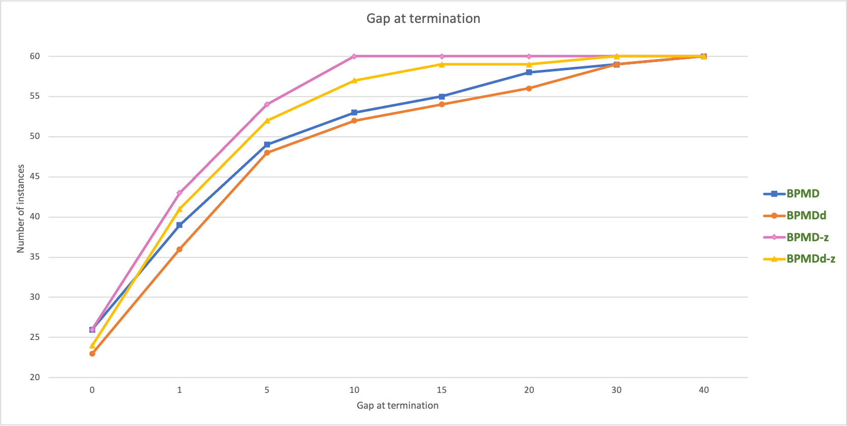
Figure 2: Cumulative chart of the number of Chao instances solved within a given gap at termination.

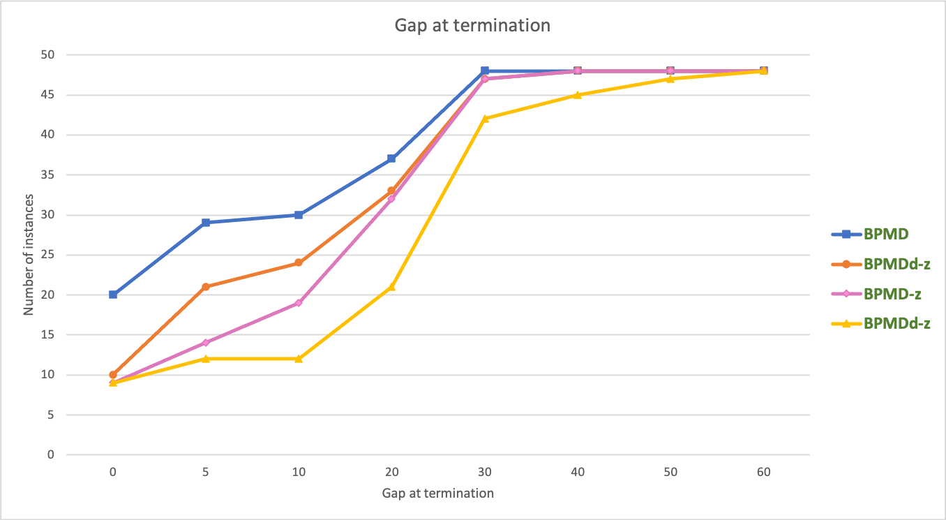
Figure 3: Cumulative chart of the number of Solomon instances solved within a given gap at termination.

We further provide two summary charts in Figures 2 and 3 related to the performance of the four models on the Chao instances and Solomon instances, respectively. They report the number of instances (on the vertical axis) for which the gap at termination is smaller than or equal to the value reported on the horizontal axis. They confirm what is shown in the summary tables presented above, since, in Figure 2 the curves associated with the models without $z$ are higher than the curves associated with the models with $z$; the opposite is true in Figure 3. In addition, we can notice that, disaggregated models $(\mathsf{{\color[rgb]{0,0.6,0}BPMD_{d}}})$ and $(\mathsf{{\color[rgb]{0,0.6,0}BPMD_{d}\text{-}z}})$ are overall performing worse than models $(\mathsf{{\color[rgb]{0,0.6,0}BPMD}})$ and $(\mathsf{{\color[rgb]{0,0.6,0}BPMD\text{-}z}})$, respectively. This might be due to the fact that the disaggregated model has more variables in the lower level. Indeed, on the one hand, these variables are also part of the single-level reformulation (due to the value-function approach), and on the other hand, they slow down the separation procedure which involves the solution of the lower level.

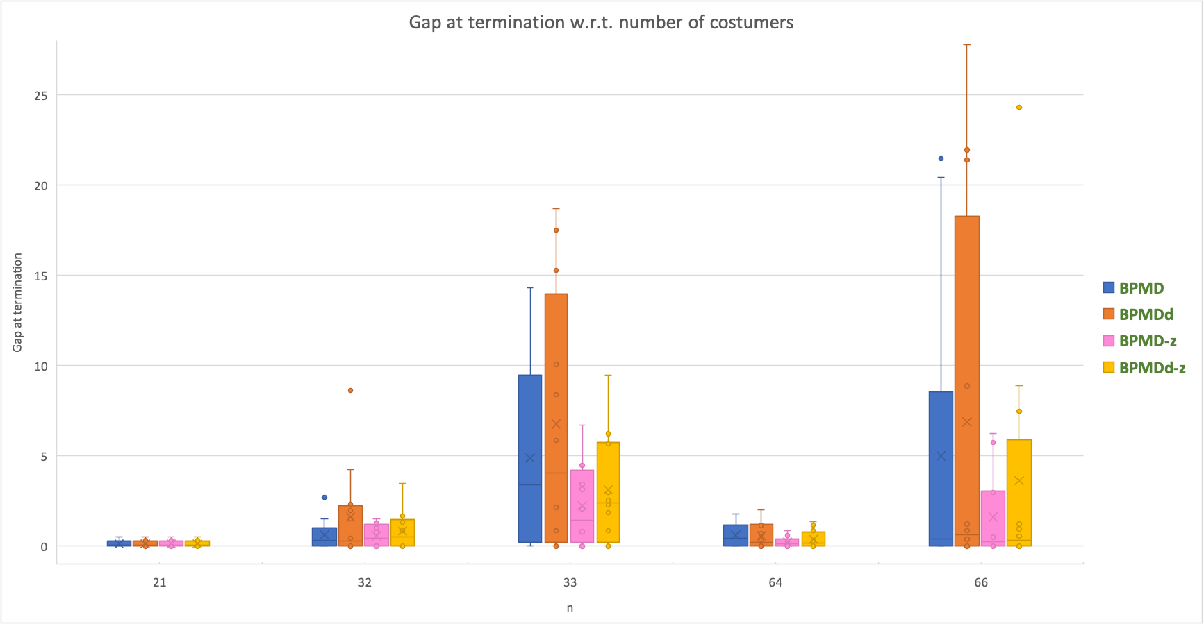
(a) Box plots obtained by aggregating the Chao instances with the same number of customers.

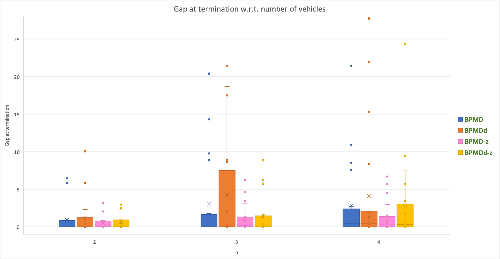
(b) Box plots obtained by aggregating the Chao instances with the same number of vehicles.

Figure 4: Box plots representing the distribution of the gap at termination of Chao instances.

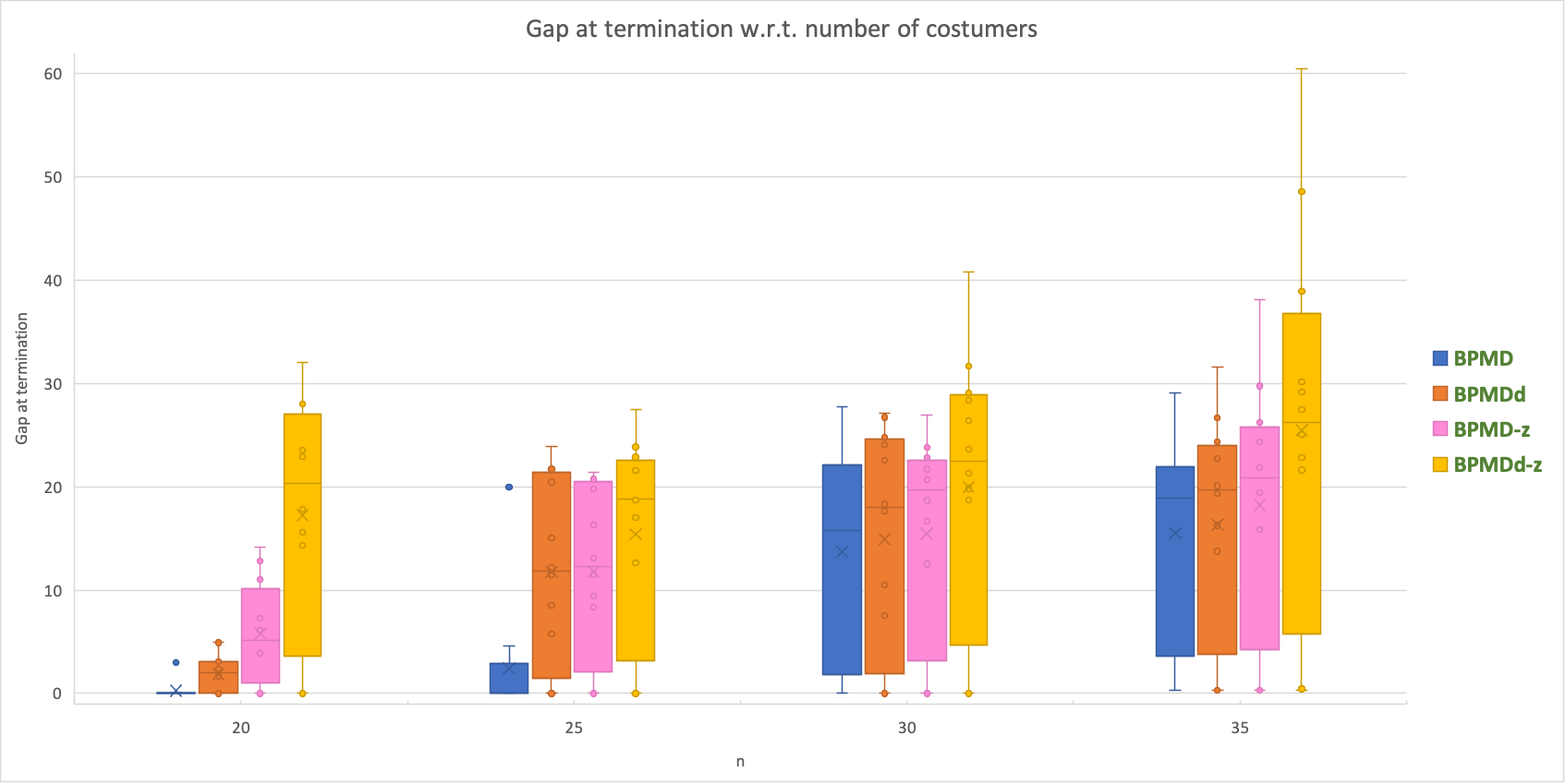
(a) Box plots obtained by aggregating the Solomon instances with the same number of customers.

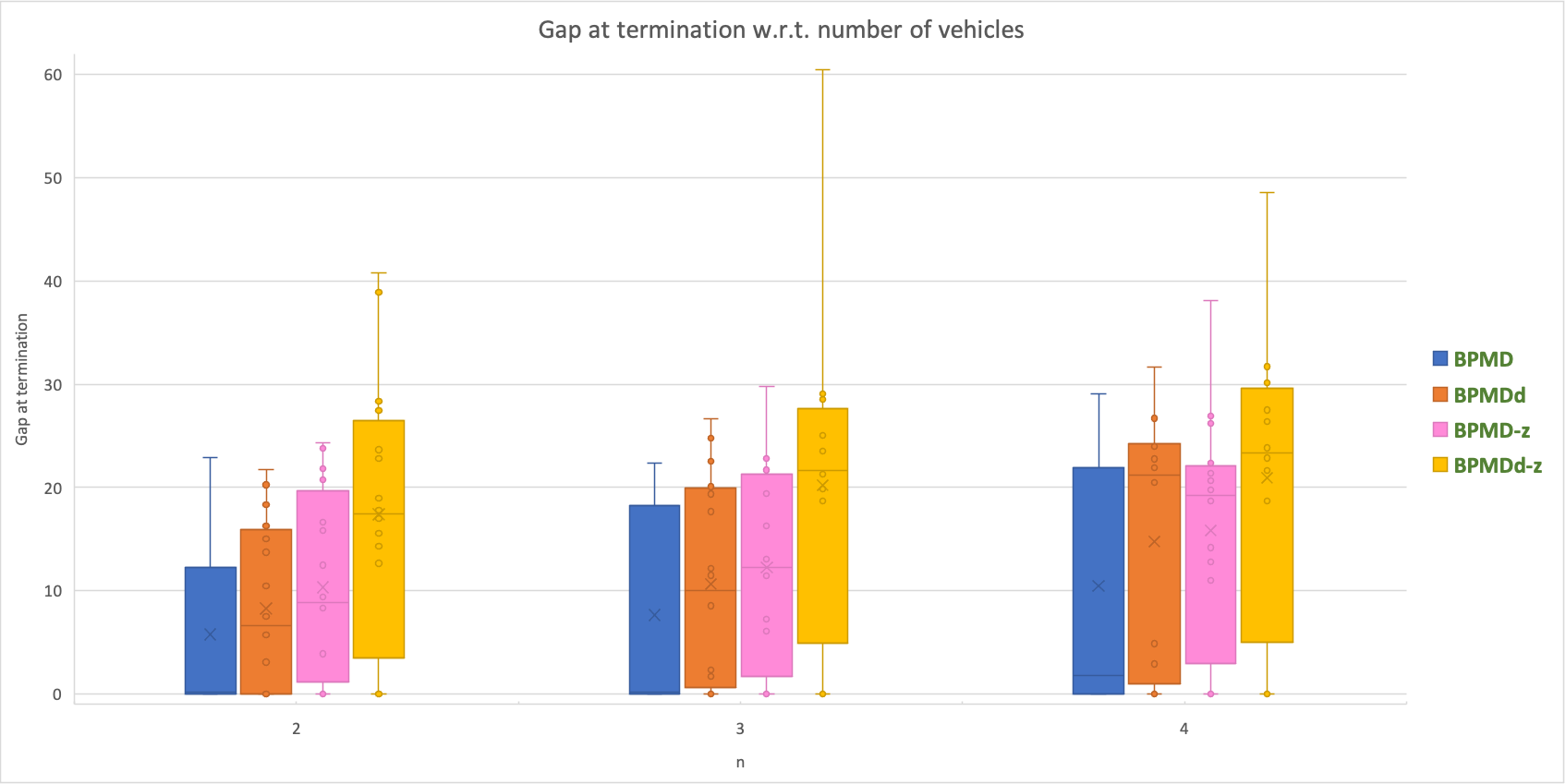
(b) Box plots obtained by aggregating the Solomon instances with the same number of customers.

Figure 5: Box plots representing the distribution of the gap at termination of Solomon instances.

In the same vein, we report four box plots representing the distribution of the gap at termination of Chao instances (Solomon instances) aggregating those with the same number of customers in Figure 4a (resp. Figure 5a), and those with the same number of vehicles in Figure 4b (resp. Figure 5b). The inter-quartile range, as well as the medians do not necessarily increase with the number of customers, since the instances have heterogeneous configurations and distances. However, for each Chao instance, the ones of models $(\mathsf{{\color[rgb]{0,0.6,0}BPMD}})$ and $(\mathsf{{\color[rgb]{0,0.6,0}BPMD_{d}}})$ are greater than the ones of the corresponding models without $z$. The opposite is true for the Solomon instances. The number of vehicles is not a crucial feature for either of the two instance types, as shown by Figures 4b and 5b.

To understand the structure of the solutions, we chose two illustrative instances, namely the Solomon instances R20_2 and R20_3, both of which could be solved to optimality by model (12) for all the tested margin values. For each of these two instances, Table 5 reports, for every tested set of margins, the profit of the leader (i.e., the optimal solution value), the percentage of items served with high, medium, and low margins respectively, the percentage of served customers, and the computational time. From this table, it is evident that the higher the considered margins are, the more diverse the solutions are, in terms of the margins applied in optimal solutions, and the more difficult is to solve them. Furthermore, for the leader, it seems more convenient to consider (i) higher margins, and (ii) a higher number of margins.

	Leader’s Profit	%high	%medium	%low	%served	time
R20_2
{0.2, 0.5}	487.5	100	-	0	100	0.1
{0.5, 0.9}	675.7	41.2	-	58.8	89.5	456
{0.2, 0.5, 0.8}	691.8	68.8	31.2	0	84.2	70
{0.5, 0.7, 0.9}	731.8	33.3	44.4	22.2	90	223
R20_3
{0.2, 0.5}	487.5	100	-	0	100	0.2
{0.5, 0.9}	661.3	41.2	-	58.8	89.5	1490
{0.2, 0.5, 0.8}	675	62.5	37.5	0	84.2	431
{0.5, 0.7, 0.9}	705.6	22.2	50	27.8	90	745

Table 5: Structure of optimal solutions of formulation $(\mathsf{{\color[rgb]{0,0.6,0}BPMD}})$ on Solomon instances R20_2 and R20_3.

6 Conclusions

The last-mile delivery field is facing an unprecedented transformation in the way operations are performed, and this is mainly caused by the explosion of e-commerce, which had huge consequences on the way the business is carried on. First, the volume of deliveries has increased: as customers are ordering online (as opposed to going directly to the shop as in offline purchases), their orders have to be dispatched to the delivery place. Second, e-buyers are more and more demanding in terms of speed of delivery. The main consequences are that demand is unpredictable and fluctuating, on one side, and consolidation opportunities are reduced, on the other side. In order to face these challenges, the companies in the field started developing new delivery strategies. One of them, which is gaining a lot of success, is related to peer-to-peer delivery, where companies (also called platforms along the paper) receive delivery requests from customers and match them with independent carriers who are available to actually perform the delivery operations. Thus, contrary to a “standard” setting, carriers are not working for the company and have their own objective, which might not coincide with the one of the company itself. Thus, the challenge for the company is maximizing the profit from the delivery operations, taking into account carriers’ objectives and behavior.

In this paper, we study a bilevel compensation and routing problem arising in peer-to-peer delivery. The problem combines the peer-to-peer logistic platform decisions about the assignment of items to the carriers and the compensation for each delivered item. The platform aims at maximizing the profit collected from delivered items, and has to take into account the carriers’ objectives when making assignment and compensation decisions. After considering the setting of fixed compensations, we propose two bilevel formulations (with aggregated and disaggregated variables) for the compensation and routing problem. These formulations are reformulated into single-level models, which are compared in terms of the quality of their linear relaxations. Equivalent formulations where routing variables are projected out are presented too. Computational tests show that the performance of the formulations depends on the features of the instances, i.e., compensation values and customers’ geography. Also, the analysis of the structure of the solutions shows that the platform might gain in offering higher compensations to carriers, which leads to a higher number of accepted offers.

Future research might develop along different avenues. One important direction would be to include stochasticity in the problem setting, especially related to carriers’ behavior. The challenge would be modeling the uncertainty, on one side, and adapting the methodologies proposed in this paper to deal with it, on the other side, or possibly, proposing ad-hoc modeling and solution approaches.

Acknowledgements: The research of E. Fernández has been partially supported through the Spanish Ministerio de Ciencia y Tecnología and European Regional Development Funds (ERDF) through project MTM2019-105824GB-I00. This support is gratefully acknowledged.

Appendix A Brief introduction to bilevel optimization

A general bilevel problem [7, 11, 12, 8, 21] is defined as a nested optimization problem where a subset of variables is constrained to be optimal for another optimization problem (the so-called lower-level problem, in contrast to the upper-level problem, which is how the outer problem is usually referred to), parametrized w.r.t. the remaining variables. It arises anytime there is a hierarchical relationship between two autonomous, and possibly conflictual, decision makers. In mathematical terms, a bilevel problem can be written as follows:

$$\begin{array}[]{rl}``\max\limits_{x\in\mathcal{X}}"&\;F(x,y)\\ s.t.&\;G(x,y)\leq 0\\ &\;y\in\arg\max\limits_{y^{\prime}\in\mathcal{Y}}\{f(x,y^{\prime})\leavevmode\nobreak\ |\leavevmode\nobreak\ g(x,y^{\prime})\leq 0\}\end{array} \mathsf{BP}$$ ()

($\mathsf{BP}$) can be seen as a Stackelberg game, where two players (a leader and a follower) make their decisions following a hierarchical order. Firstly, the leader makes his/her choice and communicates it to the follower, who will select the best response taking into account the choice of the leader. Thus, the leader’s task is to determine the optimal decision $x$, while anticipating the optimal followers’ response $y$. The $``max"$ indicates that that the problem is not well-posed if multiple optimal responses $y$ exist for a single upper-level decision $x$. In this case, one may distinguish between optimistic and pessimistic settings. In the optimistic bilevel optimization, the leader assumes that the lower-level problem will be solved in such a way as to be as beneficial as possible to the upper-level problem, i.e., maximizing its objective function. On the contrary, the pessimistic approach consists in assuming that the follower will select the optimal solution $y$ which corresponds to the worst possible outcome for the leader, in terms of the upper-level objective function.

One possible way to deal with bilevel programs is through the so-called value function reformulation. Being $\varphi(x)=\max\limits_{y^{\prime}\in\mathcal{Y}}\{f(x,y^{\prime})\leavevmode\nobreak\ |\leavevmode\nobreak\ g(x,y^{\prime})\leq 0\}$ the value function of the lower level, which gives the optimal value of the follower’s problem for any first level decision $x$, this approach consists in formulating the optimistic bilevel problem as

$$\begin{array}[]{rl}\max\limits_{x,y}&\;F(x,y)\\ s.t.&\;G(x,y)\leq 0\\ &\;g(x,y)\leq 0\\ &\;f(x,y)\geq\varphi(x)\\ &x\in\mathcal{X},y\in\mathcal{Y}.\end{array}$$

In this formulation, the lower-level constraints are lifted to the upper level, and the objective function of the lower-level problem is bounded from above by its value function.

Appendix B Formulations of $(\mathsf{{\color[rgb]{0,0.6,0}BPMD\text{-}z}})$ and $(\mathsf{{\color[rgb]{0,0.6,0}BPMD_{d}\text{-}z}})$

The formulation $(\mathsf{{\color[rgb]{0,0.6,0}BPMD\text{-}z}})$, obtained by projecting out the $z$ variables in $(\mathsf{{\color[rgb]{0,0.6,0}BPMD}})$, is:

$$\max\limits_{X,y,w,z} \quad\sum_{k\in K}\sum_{i\in V}\sum_{m\in M}p_{mi}w_{mi}^{k}$$

s.t. $$\quad\eqref{eq:pricing1-partition}\text{--}\eqref{eq:pricing1-budget},\eqref{eq:pricing1-mc1bis}\text{--}\eqref{eq:pricing1-yw},\eqref{eq:pricing1-mc2}\text{--}\eqref{eq:pricing1-mc3}$$

$$\quad y_{i}^{k}\leq\sum\limits_{m\in M}X_{mi}^{k} \quad\forall\;i\in V,k\in K$$

$$\quad\theta^{k}\geq c_{\mathsf{TSP}}(V(T))\left[\sum_{i\in V(T)}y^{k}_{i}-|V(T)|+1\right] \quad\forall\;T\in\mathcal{T},k\in K,$$

$$\quad\sum_{i\in V}\sum_{m\in M}\bar{p}_{mi}w_{mi}^{k}-\theta^{k}\geq\sum_{i\in V(T)}\sum_{m\in M}\bar{p}_{mi}X_{mi}^{k}-C^{k}(T) \quad\forall\;T\in\mathcal{T},k\in K$$

$$\quad y^{k},X_{m}^{k},w_{m}^{k}\in\{0,1\}^{n+1},\theta^{k}\in\mathbb{R} \quad\forall\;m\in M,k\in K$$

The formulation $(\mathsf{{\color[rgb]{0,0.6,0}BPMD_{d}\text{-}z}})$, obtained by projecting out the $z$ variables in $(\mathsf{{\color[rgb]{0,0.6,0}BPMD_{d}}})$, is:

$$\max\limits_{X,Y,z} \quad\sum_{k\in K}\sum_{i\in V}\sum_{m\in M}\left(p_{mi}Y^{k}_{mi}\right)$$

s.t. $$\quad\eqref{eq:pricing2-partition},\eqref{eq:pricing2-budget}$$

$$\quad Y^{k}_{mi}\leq X^{k}_{mi} \quad\forall\;i\in V,m\in M,k\in K$$

$$\quad\sum_{i\in V}\sum_{m\in M}\bar{p}_{mi}Y^{k}_{mi}-\theta^{k}\geq\sum_{i\in V(T)}\sum_{m\in M}\bar{p}_{mi}\tilde{X}^{k}_{mi}-C^{k}(T) \quad\forall\;T\in\mathcal{T},k\in K$$

$$\quad\theta^{k}\geq c_{\mathsf{TSP}}(V(T))\left[\sum_{i\in V(T)}\sum_{m\in M}Y^{k}_{mi}-|V(T)|+1\right] \quad\forall\;T\in\mathcal{T},k\in K$$

$$\quad X_{m}^{k}\in\{0,1\}^{n},Y_{m}^{k}\in\{0,1\}^{n+1},\theta^{k}\in\mathbb{R} \quad\forall\;m\in M,k\in K$$

References

- Agatz et al. [2012] N. Agatz, A. Erera, M. Savelsbergh, and X. Wang. Optimization for dynamic ride-sharing: A review. European Journal of Operational Research, 223(2):295–303, 2012. doi: 10.1016/j.ejor.2012.05.028.
- Arslan et al. [2019] A. M. Arslan, N. Agatz, L. Kroon, and R. Zuidwijk. Crowdsourced delivery—a dynamic pickup and delivery problem with ad hoc drivers. Transportation Science, 53(1):222–235, 2019. doi: 10.1287/trsc.2017.0803.
- Ausseil et al. [2022] R. Ausseil, J. A. Pazour, and M. W. Ulmer. Supplier menus for dynamic matching in peer-to-peer transportation platforms. Transportation Science, 56(5):1304–1326, 2022. doi: 10.1287/trsc.2022.1133.
- Barbosa et al. [2023] M. Barbosa, J. P. Pedroso, and A. Viana. A data-driven compensation scheme for last-mile delivery with crowdsourcing. Computers & Operations Research, 150:106059, 2023. doi: 10.1016/j.cor.2022.106059.
- Calvete et al. [2011] H. Calvete, C. Galé, and M.-J. Oliveros. Bilevel model for production-distribution planning solved by using ant colony optimization. Computers & Operations Research, 38:320–327, 01 2011. doi: 10.1016/j.cor.2010.05.007.
- Camacho-Vallejo et al. [2021] J.-F. Camacho-Vallejo, L. López-Vera, A. Smith, and J.-L. González-Velarde. A tabu search algorithm to solve a green logistics bi-objective bi-level problem. Annals of Operations Research, 07 2021. doi: 10.1007/s10479-021-04195-w.
- Candler and Norton [1977] W. Candler and R. Norton. Multi-level programming and development policy. Technical report, The World Bank Development Research Center, Washington D.C., 1977.
- Cerulli [2021] M. Cerulli. Bilevel optimization and applications. PhD thesis, Institut Polytechnique de Paris, 2021. URL http://www.theses.fr/2021IPPAX108.
- Chao et al. [1996] I.-M. Chao, B. L. Golden, and E. A. Wasil. The team orienteering problem. European Journal of Operational Research, 88(3):464–474, 1996. doi: 10.1016/0377-2217(94)00289-4.
- Cleophas et al. [2019] C. Cleophas, C. Cottrill, J. F. Ehmke, and K. Tierney. Collaborative urban transportation: Recent advances in theory and practice. European Journal of Operational Research, 273(3):801–816, 2019. doi: 10.1016/j.ejor.2018.04.037.
- Colson et al. [2007] B. Colson, P. Marcotte, and G. Savard. An overview of bilevel optimization. Annals of Operations Research, 153:235–256, 2007. doi: 10.1007/s10479-007-0176-2.
- Dempe et al. [2015] S. Dempe, V. Kalashnikov, G. A. Pérez-Valdés, and N. Kalashnykova. Bilevel Programming Problems: Theory, Algorithms and Applications to Energy Networks. Springer, Berlin, 2015. doi: 10.1007/978-3-662-45827-3.
- Du et al. [2017] J. Du, X. Li, L. Yu, R. Dan, and J. Zhou. Multi-depot vehicle routing problem for hazardous materials transportation: A fuzzy bilevel programming. Information Sciences, 399:201–218, 2017. doi: 10.1016/j.ins.2017.02.011.
- Fischetti et al. [1998] M. Fischetti, J. J. S. González, and P. Toth. Solving the orienteering problem through branch-and-cut. INFORMS Journal on Computing, 10(2):133–148, 1998. doi: 10.1287/ijoc.10.2.133.
- Fortet [1960] R. Fortet. Applications de l’algebre de boole en recherche opérationelle. Revue Française de Recherche Opérationelle, 4(14):17–26, 1960.
- Gdowska et al. [2018] K. Gdowska, A. Viana, and J. P. Pedroso. Stochastic last-mile delivery with crowdshipping. Transportation Research Procedia, 30:90–100, 2018. doi: 10.1016/j.trpro.2018.09.011. EURO Mini Conference on “Advances in Freight Transportation and Logistics”.
- Hong et al. [2019] H. Hong, X. Li, D. He, Y. Zhang, and M. Wang. Crowdsourcing incentives for multi-hop urban parcel delivery network. IEEE Access, 7:26268–26277, 2019. doi: 10.1109/ACCESS.2019.2896912.
- Horner et al. [2021] H. Horner, J. Pazour, and J. E. Mitchell. Optimizing driver menus under stochastic selection behavior for ridesharing and crowdsourced delivery. Transportation Research Part E: Logistics and Transportation Review, 153:102419, 2021. doi: 10.1016/j.tre.2021.102419.
- IBM [2017] IBM. ILOG CPLEX 12.7 User’s Manual. IBM, 2017.
- Kafle et al. [2017] N. Kafle, B. Zou, and J. Lin. Design and modeling of a crowdsource-enabled system for urban parcel relay and delivery. Transportation Research Part B: Methodological, 99:62–82, 2017. doi: 10.1016/j.trb.2016.12.022.
- Kleinert et al. [2021] T. Kleinert, M. Labbé, I. Ljubić, and M. Schmidt. A survey on mixed-integer programming techniques in bilevel optimization. EURO Journal on Computational Optimization, 9:100007, 2021. ISSN 2192-4406. doi: https://doi.org/10.1016/j.ejco.2021.100007.
- Le et al. [2019] T. V. Le, A. Stathopoulos, T. Van Woensel, and S. V. Ukkusuri. Supply, demand, operations, and management of crowd-shipping services: A review and empirical evidence. Transportation Research Part C: Emerging Technologies, 103:83–103, 2019. doi: 10.1016/j.trc.2019.03.023.
- Marinakis and Marinaki [2008] Y. Marinakis and M. Marinaki. A bilevel genetic algorithm for a real life location routing problem. International Journal of Logistics Research and Applications, 11(1):49–65, 2008. doi: 10.1080/13675560701410144.
- Marinakis et al. [2007] Y. Marinakis, A. Migdalas, and P. Pardalos. A new bilevel formulation for the Vehicle Routing Problem and a solution method using a genetic algorithm. Journal of Global Optimization, 38:555–580, 08 2007. doi: 10.1007/s10898-006-9094-0.
- Masoud and Jayakrishnan [2017] N. Masoud and R. Jayakrishnan. A decomposition algorithm to solve the multi-hop peer-to-peer ride-matching problem. Transportation Research Part B: Methodological, 99:1–29, 2017. doi: 10.1016/j.trb.2017.01.004.
- Mofidi and Pazour [2019] S. S. Mofidi and J. A. Pazour. When is it beneficial to provide freelance suppliers with choice? a hierarchical approach for peer-to-peer logistics platforms. Transportation Research Part B: Methodological, 126:1–23, 2019. doi: 10.1016/j.trb.2019.05.008.
- Nikolakopoulos [2015] A. Nikolakopoulos. A metaheuristic reconstruction algorithm for solving bi-level vehicle routing problems with backhauls for army rapid fielding. In V. Zeimpekis, G. Kaimakamis, and N. Daras, editors, Military Logistics, Operations Research/Computer Science Interfaces Series, pages 141–157. Springer Cham, 2015. doi: 10.1007/978-3-319-12075-1“˙8.
- Ning and Su [2017] Y. Ning and T. Su. A multilevel approach for modelling vehicle routing problem with uncertain travelling time. Journal of Intelligent Manufacturing, 28(3):683–688, 2017. doi: 10.1007/s10845-014-0979-3.
- Parvasi et al. [2019] S. P. Parvasi, R. Tavakkoli-Moghaddam, A. Taleizadeh, and M. Soveizy. A bi-level bi-objective mathematical model for stop location in a school bus routing problem. IFAC-PapersOnLine, 52:1120–1125, 01 2019. doi: 10.1016/j.ifacol.2019.11.346.
- Santos et al. [2021] M. J. Santos, E. Curcio, P. Amorim, M. Carvalho, and A. Marques. A bilevel approach for the collaborative transportation planning problem. International Journal of Production Economics, 233, 2021. doi: 10.1016/j.ijpe.2020.108004.
- Solomon [1987] M. M. Solomon. Algorithms for the vehicle routing and scheduling problems with time window constraints. Operations Research, 35(2):254–265, 1987. doi: 10.1287/opre.35.2.254.
- Wang et al. [2021] C. Wang, Z. Peng, and X. Xu. A bi-level programming approach to the location-routing problem with cargo splitting under low-carbon policies. Mathematics, 9:2325, 2021. doi: 10.3390/math9182325.
- Wang and Yang [2019] H. Wang and H. Yang. Ridesourcing systems: A framework and review. Transportation Research Part B: Methodological, 129:122–155, 2019. doi: 10.1016/j.trb.2019.07.009.
- Wang et al. [2018] X. Wang, N. Agatz, and A. Erera. Stable matching for dynamic ride-sharing systems. Transportation Science, 52(4):850–867, 2018. doi: 10.1287/trsc.2017.0768.