Sheaf Neural Networks for Graph-based Recommender Systems

Abstract.

Recent Graph Neural Network (GNN) advancements have facilitated widespread adoption across various applications, including recommendation systems. GNNs excel at addressing challenges posed by recommendation systems, as they can efficiently model graphs in which nodes represent users or items and edges signify preference relationships. However, current GNN techniques represent nodes by means of a single static vector, which may inadequately capture the subtle complexities of users and items. To overcome these limitations, we propose a solution integrating a cutting-edge model inspired by category theory: Sheaf Neural Networks (SNN). Unlike single vector representations, SNNs and their corresponding Laplacians represent each node (and edge) using a vector space, yielding a more comprehensive representation that can be suitably chosen during inference. This versatile method can be applied to various graph-related tasks and exhibits unparalleled performance. On the MovieLens 1M dataset, SNN exhibits more than 7.3% relative improvement on F1@10, and 2.5% relative improvement on F1@100, over the Graph Attention Network (GAT) baseline. On the Book-Crossing dataset, SNN has a relative improvement on Recall@100 of 6.8% in terms of Recall@10, and a relative improvement of 8.5% in terms of Recall@100.

Finally, we compare the run-time of our SNN model with the three most recent GNN-based models, and we observe improvements ranging from 1.5% up to 27% over the datasets we used in our experiments.

1. Introduction

Graph Neural Networks (GNNs) (Scarselli et al., 2009) have demonstrated great capabilities and reached outstanding performance in a variety of tasks, including those where their success was not given for granted. For example, Applied Calculus (Zhao et al., 2022), Drug discovery (Duvenaud et al., 2015), and Natural Language Processing (Marcheggiani and Titov, 2017).

GNNs excel in contexts where relationships are central, such as in internet information services that naturally represent relational data as graphs. For instance, social media relationships can be depicted as a unified graph, with nodes representing individuals and edges representing mutual connections.

Expanding on the idea of using graphs to represent complex relations, one of the standout real-world applications of GNNs is in collaborative filtering for recommender systems. Collaborative filtering methods work by predicting user ratings for items based on decisions made by users with similar preferences. This approach is central to many contemporary recommender systems, seen both in operational environments and at the forefront of research. These relations between users and items are often visualized as a bipartite user-item graph, where labeled edges signify observed ratings. With the rise of Deep Learning, recommendation models have reached unparalleled benchmarks (Zheng et al., 2016). In response, many businesses have adopted deep learning techniques, including GNNs (Wu et al., 2022), aiming to enhance the quality of their recommendations.

The basic idea of collaborative systems based on matrix factorization deals with the problem of “densifying” a sparse user-item matrix, where the empty entries of the matrix represent unknown ratings, and the values used to fill the empty entries are the predicted ratings for the corresponding items of a given user (Zheng et al., 2016; Shen et al., 2021). Traditional collaborative filtering methods use matrix factorization (Koren et al., 2009a) or autoencoders (Zhang et al., 2019a). GNN-based methods have been recently proposed (Han et al., 2021). These latent user and item representations are, in turn, used to reconstruct the rating, represented by the predicted weight of non-existing links in the graph using a decoder. Such weight prediction for the above-mentioned bipartite graph links can be extended to incorporate structural and external side information.

The common trait of all the above-mentioned methods is that features are represented by a precomputed and statically defined structure. For example, rows and columns of a matrix (Koren et al., 2009a), the hidden layers of an autoencoder (Zhang et al., 2019a), or factors of a tensor-like structure (Frolov and Oseledets, 2017). Being static for the above-mentioned representations means that we need additional structures (e.g., a decoder used in the GNN-based recommender system by Han et al. (Han et al., 2021)) to dynamically combine at inference time the representations in order to produce the recommendation. These additional structures, in general, represent the connections between users and items by means of learned maps that are incapable of representing the intrinsic characteristics of the connections (a sort of context such as the fact that the user in this context might prefer a particular type of item instead of another).

The additional structures used to map users to items rely on an approach called similarity-based (He et al., 2018). In a way, we could say that the mapping structure is built to adapt user-to-item representations dynamically. Better would be to have users and items representations being “raw”; in other words, instead of representing those objects by a single vector, we would need a whole vector space to capture all the possible facets of users or items and materialize the actual vectors members of the space only at inference time. This idea was introduced in a recently proposed class of GNN architectures: “Sheaf Neural Networks” (Bodnar et al., 2022).

Sheaf Neural Networks (SNNs) represent a novel class of Graph Neural Network models, drawing inspiration from Category Theory (Bodnar et al., 2022). They have been applied in various tasks and have demonstrated superiority over traditional GNNs. The foundational building blocks for these models are Cellular Sheaves. In this context, cellular sheaves allocate a vector space to every node and edge within a graph and define linear maps between these spaces. Essentially, SNNs are Graph Neural Networks that operate on Cellular Sheaves, which are vector spaces linked to the graph’s nodes. The functionality of SNNs hinges on computing a generalized version of the widely recognized Graph Laplacian, referred to as the Sheaf Laplacian (Hansen and Ghrist, 2019). The Sheaf Laplacian is genuinely a generalization of the Graph Laplacian; when the vector spaces of the cellular sheaves are confined to one dimension and identity maps are established between them, the two Laplacians align perfectly. Notably, the Sheaf Laplacian is determined non-parametrically via the restriction map during the pre-processing phase (Barbero et al., 2022).

1.1. Our Proposal

Our research extends the theoretical findings on Sheaf Neural Networks (SNNs) to the practical realm of item recommender systems. Specifically, we demonstrate that implementing SNNs in graph-based recommender systems significantly elevates their performance. Experimental results indicate that our SNN-centric models surpass all existing state-of-the-art models in their designated tasks. Notably, for recommendation tasks, our approach outdoes the leading GAT method (Veličković et al., 2017) by relative margins of 8.8% and 7.3% on the F1@10 metric for MovieLens 100k and MovieLens 1M, respectively. Additionally, we achieve a relative improvement of 8.5% in terms of Recall@100 for Book-Crossing. Our SNN model exhibits marked improvements over the latest three GNN-based models when comparing run-time efficiencies. Specifically, our method registers relative gains ranging from 1.5% to 27% compared to the second most efficient technique, GAT (Veličković et al., 2017), across the datasets used in our evaluations.

The primary original contributions of our research are as follows:

• We introduce a novel architecture for item recommender systems utilizing Sheaf Neural Networks. This method consistently attains state-of-the-art performance in its designated tasks. We further demonstrate that Sheaf Neural Networks not only offer a rigorous mathematical formalism but are also practical in scenarios where relationship information is essential for constructing holistic representations of the objects involved. This is especially true when the characteristics of these objects are ambiguous when considered in isolation.

• Through various experiments, we elucidate the relationship between our model and the application of the Bayesian Personalised Ranking loss function.

• Our extensive experimentation across multiple datasets for top-K recommendation underscores the viability and promise of our solution. Notably, our SNN-based models surpass all existing benchmarks in the focal tasks of this study. Specifically, we relatively improve the state-of-the-art method in terms of F1@10 by 8.8% on MovieLens 100k, 7.3% on MovieLens 1M, and achieve an 8.5% relative improvement in Recall@100 on Book-Crossing.

• Owing to the benefits offered by our sheaf-based architecture, recommendation computations are expedited significantly. Across the datasets employed in our studies, SNNs register relative efficiency improvements ranging from 1.5% to 27%.

2. Related work

In this section, we review the related work in the area of recommender systems. Recommender systems have been extensively studied, and various approaches have been proposed in the literature. We focus on the key developments and the most relevant work in the following areas: Autoencoder-based recommender systems, matrix factorization-based, and GNNs-based approaches.

2.1. Matrix Factorization-Based Recommender Systems

Matrix factorization (MF) is a popular collaborative filtering approach that decomposes a user-item interaction matrix into lower-dimensional latent factors. The low-rank approximation can capture the underlying structure of the data and yield better recommendations.

One of the most well-known MF-based methods is Singular Value Decomposition (SVD), which has been widely used in recommender systems. However, traditional SVD struggles with missing data, which is common in recommendation scenarios. To address this issue, Koren et al. (Koren et al., 2009b) proposed a method called SVD++ that extends the basic SVD and incorporates implicit feedback in the factorization process.

Another significant development in MF-based recommender systems is the introduction of Non-negative Matrix Factorization (NMF) by Lee and Seung (Lee and Seung, 1999). NMF imposes non-negativity constraints on the factor matrices, which can aid in interpretability and improve recommendation performance.

2.2. Autoencoder-based recommender systems

One limitation of MF-based recommender systems is their linear nature, which constrains their ability to capture complex, non-linear relationships between users and items. Additionally, these systems generally do not take into account any side information (e.g., user demographics or item attributes) that could enrich the recommendation process. Furthermore, MF methods can struggle to handle cold-start situations, where the system has little or no information about new users or items. Autoencoder-based recommender systems have emerged as a promising solution to address these limitations. Autoencoders are unsupervised learning models that aim to learn a compressed representation of input data by encoding it into a lower-dimensional space and then reconstructing the original input from the encoded representation (Zhang et al., 2019b). One of the early works in autoencoder-based recommender systems was presented by Sedhain et al (Sedhain et al., 2015), who proposed an autoencoder framework called AutoRec for CF. AutoRec learns a latent feature representation of users or items and captures the nonlinear relationships between them. Later, Liang et al. (Liang et al., 2015) introduced the Variational Autoencoder (VAE) for collaborative filtering, which learns a probabilistic latent representation to model the uncertainty in user-item preferences better. Sachdeva et al. (Sachdeva et al., 2018) implement a recurrent version of the VAE, where instead of passing a subset of the whole history regardless of temporal dependencies, they pass the consumption sequence subset through a recurrent neural network.

2.3. Graph Neural Networks-based Recommender Systems

Graph neural networks (GNNs) are a class of deep learning models that have gained attention in recent years due to their ability to handle complex relational data. They have been increasingly applied to recommender systems to exploit the graph structure of user-item relationships.

An early work in GNN-based recommender systems was presented by van den Berg et al. (van den Berg et al., 2017), who proposed a Graph Convolutional Matrix Completion (GCMC) method for link prediction in bipartite graphs. GCMC applies graph convolution operations to user-item interactions, effectively learning latent representations for recommendation. It showed improved performance compared to traditional matrix factorization-based methods that learn latent factors for users and items by factorizing the user-item interaction matrix.

NGCF (Wang et al., 2019a) designs an embedding propagation layer that refines a user’s or item’s embedding by aggregating the embeddings of the interacted items or users. By stacking multiple embedding propagation layers, the model captures collaborative signals in high-order connectivities more effectively.

In summary, GNNs have shown promising results in recommender systems by effectively modeling the complex relationships between users and items. The advancements in GNNs-based recommender systems have led to improved recommendation quality and user satisfaction.

3. Background

We briefly review the necessary background to understand the solution we propose. We start by summarizing the main characteristics of GNNs, and we then introduce cellular sheaf theory to finally present the learning algorithm we use: Neural Sheaf Diffusion. The following summarizes the main theoretical definitions and tools introduced by Barbero et al. (Barbero et al., 2022).

3.1. Graph Neural Networks

The increasing prominence of GNNs can be attributed to the advancement in both convolutional neural networks (CNNs) and Graph Representation Learning (GRL) (Wu et al., 2021). CNNs extract localized features when applied to Euclidean data, such as images or texts. However, for non-Euclidean data like graphs, CNNs need to be generalized to accommodate varying operation object sizes (e.g., pixels in images or nodes in graphs). On the other hand, GRL focuses on generating low-dimensional vector representations for nodes, edges, or subgraphs of a given graph, thus effectively capturing the intricate connectivity structures of graphs.
A graph can be denoted as $G=(V,E)$, where $V$ is the set of nodes and $E$ is the set of edges. An adjacency matrix $A$ can also describe the set of edges. Let $v_{i}\in V$ be a node and $e_{ij}=(v_{i},v_{j})\in E$ be an edge pointing from $v_{j}$ to $v_{i}$. $A$ is defined as:

(1) $$A_{ij}=\begin{cases}1\,\text{if }\,e_{ij}\in E\\ 0\,\text{otherwise}\end{cases}$$

The neighborhood of a node $v$ is denoted as:

(2) $$N(v)=\{u\in V\;|\;(v,u)\in E\}$$

The degree matrix of $G$ is a matrix $D$ that contains information about the number of edges attached to each vertex.

(3) $$D_{ij}=\begin{cases}\text{degree}(i)\,\text{if }\,i=j\\ 0\,\text{otherwise}\end{cases}$$

Using the definition of degree matrix $D$ and adjacency matrix $A$ the Laplacian can be easily defined as $L=D-A$ Given the graph data, the primary objective of GNNs is to iteratively aggregate feature information from neighbors and incorporate the aggregated information with the current central node representation during the propagation process. From a network architecture standpoint, GNNs comprise multiple propagation layers consisting of aggregation and update operations. The update operation at the $l$-th layer can be expressed as:

(4) $$H^{(l)}=f(H^{(l-1)},A)$$

where $H^{(l)}$ denotes the hidden state of nodes at layer $l$, $A$ is the adjacency matrix representing the graph structure, and $f$ is a function that combines the previous layer’s hidden state with the adjacency matrix. The aggregation operation at the $l$-th layer can be formulated as:

(5) $$H^{(l)}=\sigma\left(D_{v}^{-\frac{1}{2}}AW^{0}D_{e}^{-1}D_{v}^{-\frac{1}{2}}W^{(l)}\right),$$

where $\sigma$ is the activation function, $D_{v}$ and $D_{e}$ are the diagonal matrices of the vertex degrees and edge degrees, and $W^{(l)}$ is the learnable weight matrix at layer $l$. By stacking multiple layers of aggregation and update operations, GNNs can learn expressive node representations that effectively capture both local and global graph properties, making them suitable for graph-related tasks such as node classification, link prediction, and graph classification.

3.2. Cellular Sheaf Theory

Cellular sheaves offer a way to study graph-structured data by combining sheaf theory with graph theory. In a cellular sheaf, data is associated with the nodes and edges of a graph, representing local and global structures. This section comprehensively explains the formulation of cellular sheaves applied to graphs. We first define the data associated with the nodes and edges to construct a cellular sheaf on an undirected graph $G=(V,E)$. For each node $v\in V$, we associate a vector space or an algebraic structure, $\mathcal{F}(v)$. Similarly, for each edge $e\in E$, we associate a vector space or an algebraic structure, $\mathcal{F}(e)$. These associated spaces or structures represent the local data on the graph. We now define a restriction map, denoted by $\mathcal{F}_{v\unlhd e}:\mathcal{F}(v)\rightarrow\mathcal{F}(e)$, which represents the relationship between local data on nodes and edges for each incident node-edge pair $v\unlhd e$. Within this framework, the vector spaces corresponding to nodes and edges are called stalks, while the linear maps that connect them are known as restriction maps (Barbero et al., 2022). These restriction maps play a crucial role in transforming cellular sheaves (which in the architecture we present next represent users or items) into a tangible representation that can be utilized for generating recommendations.

For a given sheaf $(G,\mathcal{F})$, we can define the space of 0-cochains $C^{0}(G,\mathcal{F})$ as the direct sum across the vertex stalks:

(6) $$C^{0}(G,\mathcal{F})=\bigoplus_{v\in V}\mathcal{F}(v)$$

The space of 1-cochains $C^{1}(G,\mathcal{F})$ encompasses the direct sum over the edge stalks. By assigning an arbitrary orientation to each edge $e$, the co-boundary map is a linear map that relates 0-cochains to 1-cochains by capturing the difference between the data associated with the vertices connected by an edge. The co-boundary map is defined as follows:

(7) $$\delta:C^{0}(G,\mathcal{F})\rightarrow C^{1}(G,\mathcal{F})=\delta(x)_{e}=\mathcal{F}_{v\unlhd e}x_{v}-\mathcal{F}_{u\unlhd e}x_{u}$$

The sheaf Laplacian is an operator that generalizes the concept of the graph Laplacian to the setting of sheaves on graphs (Hansen and Ghrist, 2019). The graph Laplacian is a matrix that captures the connectivity structure of a graph, and it is widely used in graph analysis and spectral graph theory (Fiedler, 1973). The sheaf Laplacian extends these ideas to capture not only the graph’s connectivity but also the local-to-global relationships of the data on the graph as described by the sheaf. The sheaf Laplacian is an operator that maps 0-cochains to 0-cochains. It is defined as the composition of the co-boundary map $\delta$ and its adjoint (transpose) and is formulated as follows:

(8) $$L_{\mathcal{F}}=\delta^{T}\delta=\sum_{v,u\unlhd e}\mathcal{F}_{v\unlhd e}^{T}({F}_{v\unlhd e}x_{v}-{F}_{u\unlhd e}x_{u})$$

Notably, the sheaf Laplacian is closely related to the Laplacian, but it takes restriction maps into account instead of edges. The sheaf Laplacian captures both the graph’s connectivity structure and the local-to-global relationships of the data described by the sheaf Finally, the normalized sheaf Laplacian $\Delta_{\mathcal{F}}$ can be expressed as:

(9) $$\Delta_{\mathcal{F}}=D^{-\frac{1}{2}}L_{\mathcal{F}}D^{-\frac{1}{2}}$$

Here, $D$ represents the block-diagonal of $L_{\mathcal{F}}$ [5] which is a matrix where all the non-zero elements are arranged in square blocks along the main diagonal, and all other elements are zeros.

3.3. Neural sheaf diffusion

Consider a graph $G=(V,E)$, where $V$ represents the set of nodes and $E$ denotes the set of edges. For each individual node $v\in V$, there is an associated $d$-dimensional feature vector $x_{v}\in\mathcal{F}(v)$. In order to create an $nd$-dimensional vector $x\in C^{0}(G,\mathcal{F})$, the individual vectors $x_{v}$ are column-stacked. Following this, we generate the feature matrix $\mathbf{X}\in\mathbb{R}^{(nd)\times f}$, in which the columns of $\mathbf{X}$ are comprised of vectors belonging to $C^{0}(G,\mathcal{F})$. Sheaf diffusion can be described as a process that operates on $(G,\mathcal{F})$ and is controlled by the differential equation shown below:

(10) $$\mathbf{X}(0)=\mathbf{X},\,\,\,\,\dot{\mathbf{X}}(t)=-\Delta_{\mathcal{F}}\mathbf{X}(t)$$

This equation is discretized using the explicit Euler scheme, which employs a unit step size. The discretized version of the equation is given by:

(11) $$\mathbf{X}(t+1)=\mathbf{X}(t)-\Delta_{\mathcal{F}}\mathbf{X}(t)=(\mathbf{I}_{nd}-\Delta_{\mathcal{F}})\mathbf{X}(t)$$

In the model proposed in the paper by the authors (Bodnar et al., 2022), the discretization of the above equation is carried out as follows:

(12) $$\mathbf{X}(t+1)=\mathbf{X}(t)-\sigma(\Delta_{\mathcal{F}(t)}(\mathbf{I}_{n}\otimes\mathbf{W}_{1}^{t})\mathbf{X}_{t}\mathbf{W}_{2}^{t})$$

In this case, the sheaf $\mathcal{F}(t)$ as well as the weights $\mathbf{W}_{1}^{t}\in\mathcal{R}^{d\times d}$ and $\mathbf{W}_{2}^{t}\in\mathcal{R}^{f_{1}\times f_{2}}$ are time-dependent. This implies that the underlying geometric structure of the graph changes over time.

4. Method

4.1. Collaborative filtering

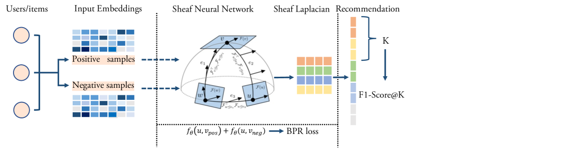
Figure 1. Complete representation of our approach. Initially, are computed the input embeddings related to positive and negative samples. The output of these embeddings is taken as input from SNN (taken from (Bodnar et al., 2022), and finally, the predictions of SNN are used to compute the performance metrics.

We combine cellular sheaves with the Bayesian Personalized Ranking (BPR) loss to implement our novel recommender system framework. The cellular sheaf provides a formalism to organize the relationships between users, items, and preference scores, enabling a structured representation of the underlying problem setting. Given a bipartite graph $G=(W,E)$, where $W=U\cup V$ represents the disjoint union of the user vertex set $U$. The item vertex set $V$, we construct a cellular sheaf $\mathcal{F}$ on the graph, where 0-cochains are naturally associated with the latent factors (embeddings) of users and items, and 1-cochains naturally represent the observed preference scores. By harnessing the sheaf structure, our objective is to compute latent factors, capitalizing on the rationale inherent to the BPR loss optimization. This loss emphasizes the probability of a user favoring a positively observed item over a randomly selected negative counterpart. Our methodology introduces a fresh viewpoint on personalized ranking within recommender systems by merging the robust expressiveness of the cellular sheaf framework with the established efficacy of the BPR loss.

User nodes serve as input embeddings provided to the model in the input layer. We generate random embeddings for each user and item in the graph to initialize the model. Subsequently, we sample both positive and negative interactions to train the model. Following the input layer, a new item embedding is created and passed to Layer 1. The user node embedding is then updated with a new item embedding containing semantic information related to its connected users. It is important to note that during this layer, nodes learn not only from the embedding obtained in the input layer but also from this new embedding. In Layer 2, the previous item embedding is updated with a new one. Through this approach, we aim to cluster users with similar item interests.

As a result, the user node in the final layer will also represent the knowledge about the users that are up to 2-hops away in the Graph. In the context of recommendations, this process makes the user’s node embedding more similar to other users who share the same item interests. The rationale behind the choice of node embedding is clear-cut: an embedding vector is generated for each node in the graph. This embedding vector can capture the graph representation and structure. At each step, the user’s node embedding becomes more similar to other users who share the same item interests. Essentially, nodes in close proximity should also have vectors in close proximity to each other.

One advantage of our approach lies in the connection between the proposed embedding and the architecture. The SNN accepts an embedding vector as input, which contains a modified representation of users and items, along with the size of the graph (the sum of the number of users and items). Following this, all the information from the embedding is stored in the corresponding vector spaces. The entire process can be seen in Figure 1.

4.1.1. Loss function

The Bayesian Personalized Ranking (BPR) loss is a natural selection for the loss function in Recommender Systems. To fully understand BPR, we must elucidate the notions of positive and negative edges. Positive edges correspond to user actions, such as purchasing or selecting an item, and are, therefore, present in the graph. In contrast, negative interactions are unobservable, meaning negative edges are absent from the graph. Within the framework of Sheaf Neural Networks applied to our bipartite graph, the score for user $u$ regarding item $v$ can be expressed as the scalar product of the two nodes. This is achieved by multiplying their respective values in the 0-cochain: $f_{\theta}(u,v)=\mathcal{F}_{u}^{T}\mathcal{F}_{v}$.

Here, $\mathcal{F}_{u}$ represents the embedding learned for user $u$, and $\mathcal{F}_{v}$ represents the learned embedding associated with item $v$. Subsequently, for user $u$, we can define the set of all positive edges containing $u$ as $s(p)=f_{\theta}(u,v_{pos})$ and the set of all negative edges containing $u$ as $s(n)=f_{\theta}(u,v_{neg})$. The BPR is given by:

(13) $$BPR(u)=\sum_{p,n}-ln(\sigma(s(p)-s(n))$$

We train the model using mini-batch sampling to estimate the BPR loss and optimize $f_{\theta}$. For each mini-batch, we sample a set of users, and for each user, we sample one positive item (the item from a positive edge containing the user in question) and one negative item.

4.2. SheafNN and Recommendation

4.2.1. SheafConvNet

We study the diffusion-type model proposed by (Bodnar et al., 2022) for the task of recommendation. Given a graph $G(V,E)$ with $|V|=N$ nodes and $|E|$ edges, let $X\in\mathbb{R}^{N\times d}$ represent the node features, where $d$ is the feature dimension. To effectively learn each $d\times d$ matrix $\mathcal{F}_{v\unlhd e}x_{v}$, the sheaf diffusion layer makes use of a sheaf learner for calculating the parametric restriction map, symbolized by $\mathcal{S}(X{u},X_{v})=\tanh(W_{\mathcal{F}}(X_{u}\oplus X_{v}))$.

In this equation, $\oplus$ represents the concatenation operation, which merges the source node $X_{u}$ features and the target node $X_{v}$. The $\tanh$ function is applied element-wise, infusing nonlinearity into the model and consequently enabling it to learn more intricate mappings. The weight matrix $W_{\mathcal{S}}$ is obtained during the training phase. The resulting output is a single scalar value, which signifies the restriction map for the respective edge.

The intuition is that by using the node features for the edge source and target, the model can learn edge weights that depend on the semantic content and attributes of the nodes. Edges between similar nodes may have high weights, while edges between dissimilar nodes may have low weights. The tanh activation constrains the weights to the range (-1, 1).

At a high level, the goals of learning the restriction maps are:

• Learn an adaptive adjacency matrix that depends on the node features rather than a fixed adjacency. This allows the model to adapt the graph structure to the node attributes.

• Filter out noisy or unimportant edges by assigning them very low weights while keeping important edges. This acts as a kind of ”soft” edge pruning mechanism.

The restriction maps are used to build the graph Laplacian matrix, which is then used for message passing to update the node features. Specifically, the restriction maps $\mathcal{S}$ are used to build an adjacency matrix $A$ where $A_{uv}=-\mathcal{S}(X_{u},X_{v})$ if edge $uv$ connects node $u$ to node $v$, and 0 otherwise. The adjacency matrix $A$ is used to construct a normalized Laplacian matrix $\mathcal{L}=D^{-1/2}(A+I)D^{-1/2}$, where $D$ is the degree matrix of $A$. The Laplacian $\mathcal{L}$ is used for message passing to update the node features: $X^{t+1}=X^{t}-\alpha\mathcal{L}X^{t}$, where $\alpha$ is a step size hyperparameter. The updated node features $X^{t+1}$ are used as predictions or passed to subsequent SheafConvLayers.

4.2.2. Recommendation

Before training, we associate two nodes $u,v$ with their respective users. Each node is split into two partitions. One containing positive samples, i.e., pairs of nodes where interactions were positive (meaning, user positively rating an item) or negative. As stated above, $f_{\theta}(u,v)=\mathcal{X}_{u}^{T}\mathcal{X}_{v}$ is the score for the user $u$ and item $v$. After the last diffusion layer, the score can be easily obtained through the restriction maps $\mathcal{F}{u\unlhd e}$ and $\mathcal{F}{v\unlhd e}$ which are matrices of shapes $d_{e}\times d_{u}$ and $d_{v}\times d_{e}$. With this representation, the computation becomes extremely straightforward.

As discussed in (Barbero et al., 2022), the sheaf framework could not be directly applied to bipartite graphs. Consequently, we adapted the sheaf Laplacian operator to fit the structure of bipartite graphs. We devised a simple sheaf diffusion process for model training derived from the sheaf Laplacian. This approach facilitates parameter updates while preserving the intrinsic properties of the sheaf.

5. Experiments

In this section, we test the performance of Sheaf Neural Networks on collaborative filtering. We use the following datasets: MovieLens 1M, and Book-Crossing. We also run experiments on MovieLens 100K but we report the full results in the Supplemental Material.

5.1. Datasets description

5.1.1. MovieLens

The MovieLens 1M dataset comprises about 1 million anonymous ratings from 6040 users for nearly 3900 movies. Each user has rated a minimum of 20 movies. Similarly, the MovieLens 100k dataset contains approximately 100,000 anonymous ratings from 1000 users for about 1700 movies, with each user rating at least 20 movies. Ratings in both the MovieLens 1M and MovieLens 100K datasets are given on a 5-star scale, with half-star increments. Both datasets also provide demographic information for each user, including age, gender, and occupation.
Building on the data from the MovieLens datasets, one can utilize a bipartite graph to effectively visualize the interactions between users and movies. In such a graph, both users and movies are represented as nodes, and the edges connecting them denote user-movie interactions. The nature of this graph is bipartite: while users can express interest in movies, movies don’t reciprocate interest in users, and similarly, users don’t express interest in other users.

5.1.2. Book-Crossing dataset

The Book-Crossing dataset (Ziegler et al., 2005) compiles user ratings for books. These ratings are of two types: explicit ratings, which range from 1 to 10 stars, and implicit ratings, which merely indicate a user’s interaction with a book. This dataset encompasses ratings from 278,858 Book-Crossing members and consists of 1,157,112 ratings pertaining to 271,379 unique ISBNs.

5.2. Baselines

We compare our model with various baselines, including current state-of-the-art models, including recently published neural architectures. We now briefly summarize the models we use as baselines in our experiments.

• CoFM (Piao and Breslin, 2018) jointly trains FM and TransE by sharing parameters or regularization of aligned items and entities.

• MVAE (Liang et al., 2018) is an extension of variational autoencoders (VAEs) to collaborative filtering for implicit feedback.

• SVAE (Sachdeva et al., 2018) is an improvement of MVAE using sequential VAEs based on a recurrent neural network.

• LinUCB (Li et al., 2010) is a multi-armed bandit approach that recommends items to the user based on the contextual information about the user and items.

• SVD (Polat and Du, 2005) is a popular algorithm utilizing Singular Value Decomposition for the process of recommendation.

• DeepMF (Xue et al., 2017) is a state-of-the-art neural network architecture based Matrix Factorization Recommendation Method.

• MDP (Padhye et al., 2022) works as a reinforcement learning agent modeling collaborative filtering as a Markov Decision Process (MDP).

• LibFM (Niepert et al., 2016) is a widely used feature-based factorization model for CTR prediction.

• RippleNet (Wang et al., 2018) is a memory-network-like approach that propagates users’ preferences on the KG for recommendation.

• KGNN-LS (Wang et al., 2019b) transforms the graph into a weighted graph and uses a GNN to compute item embeddings.

• NGCF (Wang et al., 2019a) consists of a recent collaborative filtering algorithm implemented using a neural network.

• LightGCN (He et al., 2020) is a form of Graph Convolutional Neural network (GCN), which includes the neighborhood aggregation for collaborative filtering, the most crucial part of GCN.

• GAT (Veličković et al., 2017) is the popular Graph Attention Network architecture we adapted to serve as a collaborative filtering method on graph data.

5.3. Metrics

We use three evaluation metrics that have been widely used in previous work:

• Precision@K: It is the fraction of the items recommended that are relevant to the user. We compute the mean of all the users as final precision;

• Recall@K: The proportion of items relevant to the user has been successfully recommended. We compute the mean of all users as final recall.

• F1-score@K: The harmonic mean of precision and recall at rank K.

We also report on the time in seconds necessary to produce 100 recommendations. We compare SSN, our method, against the three main SOTA graph-based recommender systems, namely NGCF (Wang et al., 2019a), LightGCN (He et al., 2020), and GAT (Veličković et al., 2017).

Finally, to show that BPR loss is the correct choice for the SNN architecture on the the recommendation task, we also compare the F1-Score@10 on MoviLens 1M when SNN is trained using the two most popularly used losses, namely Root Mean Squared Error (RMSE) and Binary Cross-Entropy (BCE).

6. Results

6.1. MovieLens 1M

In this section, we test the performance of SNN on MovieLens 1M. We used a 90-10 train-test split. 90% of the samples are used for training and 10% for testing. During the comparison, the learning rate and the weight decay are fixed and equal to $0.005$ and $0.0001$. The model training process ends in 210 minutes in total. The selected size for the embedding vector is 64; consequently, the input size of SNN is 64. We set to 5 the number of SNN layers. See Section 6.5 for detail on the impact of the number of layers on performance.

In Figure 2, we juxtapose the F1-Score of SNN with that of other state-of-the-art systems as we vary $K$, the number of recommendations generated. It’s evident that SNN consistently outshines the baselines; its F1-Score@K remains superior to all other methods for each distinct value of $K$.

Table 1 shows that SNN outperforms all the baselines both in terms of F1-Score, and Recall.

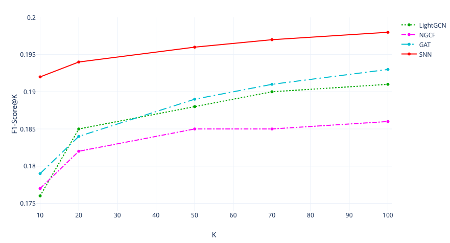
Figure 2. F1-Score values on MovieLens 1M compared with state-of-the-art solutions. The value of F1-Score for SNN is always higher than the other approaches for all the values of K (number of generated recommendations).

This experiment shows that this architecture can achieve good results also for high values of $K$. the number of generated recommendations. This is consistent with the typical two-tier software architecture used in modern recommender (Hron et al., 2020) systems where a first tier retrieves the recommendations (our module) and a second tier reranks it afterward. A higher value of Recall score, as it is our case when $K$ is large is thus preferable. We observe an improvement of up to 7% in F1-Score@10 and up to 2.5% in F1-Score@100 for SNN compared to its closest competitor, GAT. As the table indicates, when $K$ is small, SNN’s primary advantage over the baselines is its adeptness at balancing precision and recall. In real-world scenarios with a single-stage recommender system, this balance becomes critical. The goal is often to deliver precise recommendations while ensuring no potentially valuable items are missed, especially when the number of recommendations increases.

Model	Precision@10	Recall@10	F1-Score@10	Precision@100	Recall@100	F1-Score@100
MVAE†	0.090	0.091	0.091	0.054	0.414	0.096
SVAE†	0.144	0.125	0.134	0.069	0.494	0.121
CoFM†	0.321	0.130	0.178	0.354	0.135	0.189
LightGCN	0.199	0.159	0.176	0.128	0.376	0.191
NGCF	0.134	0.261	0.177	0.117	0.458	0.186
GAT	0.143	0.239	0.179	0.123	0.454	0.193
SNN (ours)	0.284	0.145	0.192	0.124	0.518	0.198

Table 1. Results of the evaluation using the MovieLens 1M dataset. SNN exhibits more than 7.3% relative improvement on F1@10, and 2.5% relative improvement on F1@100, over the Graph Attention Network (GAT) baseline. †  is used when the results are taken from the original paper.

6.2. Book-Crossing

For this experiment, both the learning rate and the weight decay were set to $0.001$ and $0.0005$, respectively. The model underwent training for 70 epochs, taking a computational time of 251 minutes, and utilized the BPR loss as its loss function. The longer computational time, compared to our previous experiments, is attributed to the larger dataset size enriched with extensive side information, thereby necessitating more processing time. In this specific experiment, an optimal result was achieved by setting the embedding vector size to 32. We focused on Recall@10 and Recall@100 metrics, as these are the standard measurements for this dataset (Wang et al., 2018, 2019b; Niepert et al., 2016). This focus allowed us to compare our findings with those documented in the original papers detailing the technique.

Referring to Table 2, our approach surpasses the state-of-the-art in both Recall@10 and Recall@100 metrics. Specifically, SNN betters the Recall@10 of LightGCN by approximately $7$%, and it enhances the Recall@100 by around $8.6$%.

Model	Recall@10	Recall@100
SVD	0.046	0.109
LibFM†	0.062	0.124
GAT	0.071	0.123
RippleNet†	0.074	0.127
KGNN-LS†	0.082	0.149
NGCF	0.085	0.157
LightGCN	0.087	0.163
SNN (ours)	0.093	0.177

Table 2. Results of the evaluation using the Book-Crossing dataset. SNN has a relative improvement on Recall@100 of 6.8% in terms of Recall@10, and a relative improvement of 8.5% in terms of Recall@100. †  means that we use the results reported in the original paper describing the model.

6.3. MovieLens 100K

For a comprehensive analysis, we also conducted experiments on the 100K version of the dataset. Interestingly, we did not observe any significant differences compared to the results from the 1M version.

In brief, We improve F1-Score@10 by approximately 9% when we compare SNN over GAT (the second best). In terms of F1-Score@20 we can observe an improvement of about 2.5% over GAT. Please see the Supplementary Material for more detailed results.

6.4. Impact of the BPR Loss

We show that BPR is the best loss to train SNN compared to two popularly used losses: the Root Mean Squared Error (RMSE) and the Binary Cross-Entropy (BCE). We compute F1-Score@10 on the MovieLens 1M dataset, showing in Table 3 that this metric is worse when SNN is trained using RMSE or BCE. For the sake of completeness, we also varied the number of layers of each architecture to balance possible negative effects on the performance due to the depth of the network.

Additionally, the last column of Table 3 highlights that BPR has a computational edge over RMSE and BCE in terms of the training time required for the model.

Loss	#Layers	F1-Score@10	Time
RMSE	2	0.112	283
RMSE	5	0.148	371
BCE	2	0.087	198
BCE	5	0.101	262
BPR	2	0.163	163
BPR	5	0.192	210

Table 3. Performance in terms of F1-Score@10 of SNN when using different loss functions and numbers of layers. The training time is in minutes, therefore smaller is better.

6.5. Number of Layers

A distinctive advantage of SNN is its capability to mitigate over-smoothing by supporting the integration of numerous sheaf layers (Bodnar et al., 2022). Contrarily, in many GNN architectures, it has been previously demonstrated (Oono and Suzuki, 2019) that the algorithm’s performance diminishes with the augmentation of layer count.

We evaluated the F1-Score@10 across varying layer counts, ranging from 2 to 5. As depicted in Figure 3, optimal performance is typically achieved when the number of layers is set to 5.

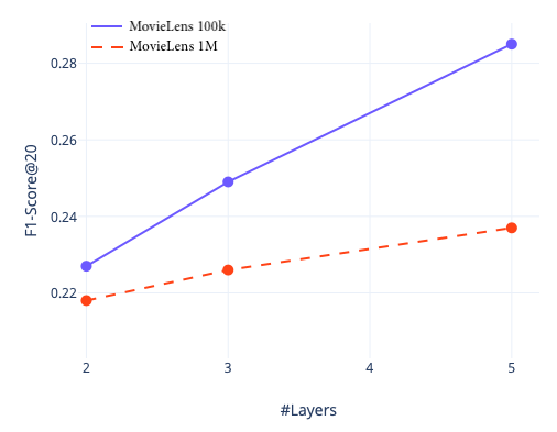
Figure 3. Values of F1-Score on MovieLens 100k depending on the number of layers. Our network is robust with respect to over-smoothing problems that are common in GNNs

6.6. Recommendation Time

In Table 4, we compare the recommendation time of SNN against other state-of-the-art methods. For a fair comparison, we used the same number of layers (set to 5), held the hyperparameters constant, and measured computational time in seconds. Clearly, SNN outperforms all other methods, showcasing the shortest computational time. Despite its complex topological structure, our method remains stable and consistently achieves top-tier performance.

Model	MovieLens 1M	Book-Crossing
GAT	9.226	12.010
NGCF	8.964	12.734
LightGCN	11.254	15.131
SNN (ours)	$\mathbf{8.827}$	$\mathbf{11.439}$

Table 4. Time required to give the top 100 recommendations to a user (in seconds) compared with LightGCN and NGCF. Our solution outperforms both the approaches on the three datasets. $\downarrow$ is better.

7. Conclusions and future work

Our SNN architecture allows the utilization of vector spaces, not just ’simple’ vectors, to represent nodes and edges in bipartite graphs of user-item interactions. Experimental results highlight SNN’s consistent superiority over top-performing baseline models, improving F1@10 by a relative 8.8% on MovieLens 100k and a relative 7.3% on MovieLens 1M, and relatively boosting Recall@100 by 8.5% on Book-Crossing.

The central thesis of this paper is the potential of novel architectures grounded in Sheaf theory. These architectures are particularly suited for contexts where relationships and their representations hinge on intricate latent factors and are intrinsically ambiguous. Take, for instance, a user’s behavior, which is influenced by the items they interact with. A mere vector may fall short in capturing the nuances of such behaviors, suggesting that a full vector space might be more apt. This reasoning could extend to various application domains. Looking forward, we aim to adapt this architecture to broader research spheres. Its unique topological nature implies versatility, especially when embedding side information in related stalks. A viable avenue worth exploration is the Next Point-Of-Interest recommendation system, which could advise users by leveraging historical data and immediate inclinations.

References

- (1)
- Barbero et al. (2022) Federico Barbero, Cristian Bodnar, Haitz Sáez de Ocáriz Borde, Michael Bronstein, Petar Veličković, and Pietro Liò. 2022. Sheaf Neural Networks with Connection Laplacians. , 28–36 pages.
- Bodnar et al. (2022) Cristian Bodnar, Francesco Di Giovanni, Benjamin Paul Chamberlain, Pietro Liò, and Michael M. Bronstein. 2022. Neural Sheaf Diffusion: A Topological Perspective on Heterophily and Oversmoothing in GNNs. https://doi.org/10.48550/ARXIV.2202.04579
- Duvenaud et al. (2015) David K Duvenaud, Dougal Maclaurin, Jorge Iparraguirre, Rafael Bombarell, Timothy Hirzel, Alán Aspuru-Guzik, and Ryan P Adams. 2015. Convolutional networks on graphs for learning molecular fingerprints. Advances in neural information processing systems 28 (2015).
- Fiedler (1973) Miroslav Fiedler. 1973. Algebraic connectivity of graphs. Czechoslovak Mathematical Journal 23, 2 (1973), 298–305. http://eudml.org/doc/12723
- Frolov and Oseledets (2017) Evgeny Frolov and Ivan Oseledets. 2017. Tensor methods and recommender systems. Wiley Interdisciplinary Reviews: Data Mining and Knowledge Discovery 7, 3 (2017), e1201.
- Han et al. (2021) Soyeon Caren Han, Taejun Lim, Siqu Long, Bernd Burgstaller, and Josiah Poon. 2021. Glocal-k: Global and local kernels for recommender systems. , 3063–3067 pages.
- Hansen and Ghrist (2019) Jakob Hansen and Robert Ghrist. 2019. Toward a spectral theory of cellular sheaves. Journal of Applied and Computational Topology 3 (2019), 315–358.
- He et al. (2020) Xiangnan He, Kuan Deng, Xiang Wang, Yan Li, Yongdong Zhang, and Meng Wang. 2020. LightGCN.
- He et al. (2018) Xiangnan He, Zhankui He, Jingkuan Song, Zhenguang Liu, Yu-Gang Jiang, and Tat-Seng Chua. 2018. NAIS: Neural Attentive Item Similarity Model for Recommendation. , 2354–2366 pages. https://doi.org/10.1109/tkde.2018.2831682
- Hron et al. (2020) Jiri Hron, Karl Krauth, Michael I Jordan, and Niki Kilbertus. 2020. Exploration in two-stage recommender systems. stat 1050 (2020), 1.
- Koren et al. (2009a) Yehuda Koren, Robert Bell, and Chris Volinsky. 2009a. Matrix factorization techniques for recommender systems. Computer 42, 8 (2009), 30–37.
- Koren et al. (2009b) Yehuda Koren, Robert Bell, and Chris Volinsky. 2009b. Matrix Factorization Techniques for Recommender Systems. Computer 42, 8 (2009), 30–37. https://doi.org/10.1109/MC.2009.263
- Lee and Seung (1999) D D Lee and H S Seung. 1999. Learning the parts of objects by non-negative matrix factorization. Nature 401, 6755 (Oct. 1999), 788–791.
- Li et al. (2010) Lihong Li, Wei Chu, John Langford, and Robert E. Schapire. 2010. A contextual-bandit approach to personalized news article recommendation. https://doi.org/10.1145/1772690.1772758
- Liang et al. (2015) Dawen Liang, Laurent Charlin, James McInerney, and David M Blei. 2015. Modeling User Exposure in Recommendation. arXiv:stat.ML/1510.07025
- Liang et al. (2018) Dawen Liang, Rahul G. Krishnan, Matthew D. Hoffman, and Tony Jebara. 2018. Variational Autoencoders for Collaborative Filtering. https://doi.org/10.48550/ARXIV.1802.05814
- Marcheggiani and Titov (2017) Diego Marcheggiani and Ivan Titov. 2017. Encoding Sentences with Graph Convolutional Networks for Semantic Role Labeling. In Proceedings of the 2017 Conference on Empirical Methods in Natural Language Processing. Association for Computational Linguistics, Copenhagen, Denmark, 1506–1515. https://doi.org/10.18653/v1/D17-1159
- Niepert et al. (2016) Mathias Niepert, Mohamed Ahmed, and Konstantin Kutzkov. 2016. Learning Convolutional Neural Networks for Graphs. https://doi.org/10.48550/ARXIV.1605.05273
- Oono and Suzuki (2019) Kenta Oono and Taiji Suzuki. 2019. Graph Neural Networks Exponentially Lose Expressive Power for Node Classification. https://doi.org/10.48550/ARXIV.1905.10947
- Padhye et al. (2022) Vaibhav Padhye, Kailasam Lakshmanan, and Amrita Chaturvedi. 2022. Proximal policy optimization based hybrid recommender systems for large scale recommendations. https://doi.org/10.1007/s11042-022-14231-x
- Piao and Breslin (2018) Guangyuan Piao and John G. Breslin. 2018. Transfer Learning for Item Recommendations and Knowledge Graph Completion in Item Related Domains via a Co-Factorization Model. In The Semantic Web, Aldo Gangemi, Roberto Navigli, Maria-Esther Vidal, Pascal Hitzler, Raphaël Troncy, Laura Hollink, Anna Tordai, and Mehwish Alam (Eds.). Springer International Publishing, Cham, 496–511.
- Polat and Du (2005) Huseyin Polat and Wenliang Du. 2005. SVD-Based Collaborative Filtering with Privacy. , 5 pages. https://doi.org/10.1145/1066677.1066860
- Sachdeva et al. (2018) Noveen Sachdeva, Giuseppe Manco, Ettore Ritacco, and Vikram Pudi. 2018. Sequential Variational Autoencoders for Collaborative Filtering. https://doi.org/10.48550/ARXIV.1811.09975
- Scarselli et al. (2009) Franco Scarselli, Marco Gori, Ah Chung Tsoi, Markus Hagenbuchner, and Gabriele Monfardini. 2009. The Graph Neural Network Model. IEEE Transactions on Neural Networks 20, 1 (2009), 61–80. https://doi.org/10.1109/TNN.2008.2005605
- Sedhain et al. (2015) Suvash Sedhain, Aditya Krishna Menon, Scott Sanner, and Lexing Xie. 2015. AutoRec: Autoencoders Meet Collaborative Filtering. In Proceedings of the 24th International Conference on World Wide Web (WWW ’15 Companion). Association for Computing Machinery, New York, NY, USA, 111–112.
- Shen et al. (2021) Wei Shen, Chuheng Zhang, Yun Tian, Liang Zeng, Xiaonan He, Wanchun Dou, and Xiaolong Xu. 2021. Inductive Matrix Completion Using Graph Autoencoder. https://doi.org/10.48550/ARXIV.2108.11124
- van den Berg et al. (2017) Rianne van den Berg, Thomas N Kipf, and Max Welling. 2017. Graph Convolutional Matrix Completion. arXiv:stat.ML/1706.02263
- Veličković et al. (2017) Petar Veličković, Guillem Cucurull, Arantxa Casanova, Adriana Romero, Pietro Liò, and Yoshua Bengio. 2017. Graph Attention Networks. https://doi.org/10.48550/ARXIV.1710.10903
- Wang et al. (2018) Hongwei Wang, Fuzheng Zhang, Jialin Wang, Miao Zhao, Wenjie Li, Xing Xie, and Minyi Guo. 2018. RippleNet. https://doi.org/10.1145/3269206.3271739
- Wang et al. (2019b) Hongwei Wang, Fuzheng Zhang, Mengdi Zhang, Jure Leskovec, Miao Zhao, Wenjie Li, and Zhongyuan Wang. 2019b. Knowledge-aware Graph Neural Networks with Label Smoothness Regularization for Recommender Systems. https://doi.org/10.48550/ARXIV.1905.04413
- Wang et al. (2019a) Xiang Wang, Xiangnan He, Meng Wang, Fuli Feng, and Tat-Seng Chua. 2019a. Neural Graph Collaborative Filtering. arXiv:cs.IR/1905.08108
- Wu et al. (2022) Shiwen Wu, Fei Sun, Wentao Zhang, Xu Xie, and Bin Cui. 2022. Graph neural networks in recommender systems: a survey. Comput. Surveys 55, 5 (2022), 1–37.
- Wu et al. (2021) Zonghan Wu, Shirui Pan, Fengwen Chen, Guodong Long, Chengqi Zhang, and Philip S. Yu. 2021. A Comprehensive Survey on Graph Neural Networks. IEEE Transactions on Neural Networks and Learning Systems 32, 1 (2021), 4–24. https://doi.org/10.1109/TNNLS.2020.2978386
- Xue et al. (2017) Hong-Jian Xue, Xin-Yu Dai, Jianbing Zhang, Shujian Huang, and Jiajun Chen. 2017. Deep Matrix Factorization Models for Recommender Systems. , 7 pages.
- Zhang et al. (2019a) Guijuan Zhang, Yang Liu, and Xiaoning Jin. 2019a. A survey of autoencoder-based recommender systems. Frontiers of Computer Science 14 (08 2019). https://doi.org/10.1007/s11704-018-8052-6
- Zhang et al. (2019b) Shuai Zhang, Lina Yao, Aixin Sun, and Yi Tay. 2019b. Deep Learning Based Recommender System. Comput. Surveys 52, 1 (feb 2019), 1–38. https://doi.org/10.1145/3285029
- Zhao et al. (2022) Qingqing Zhao, David B. Lindell, and Gordon Wetzstein. 2022. Learning to Solve PDE-constrained Inverse Problems with Graph Networks. https://doi.org/10.48550/ARXIV.2206.00711
- Zheng et al. (2016) Yin Zheng, Bangsheng Tang, Wenkui Ding, and Hanning Zhou. 2016. A Neural Autoregressive Approach to Collaborative Filtering. https://doi.org/10.48550/ARXIV.1605.09477
- Ziegler et al. (2005) Cai-Nicolas Ziegler, Sean M. McNee, Joseph A. Konstan, and Georg Lausen. 2005. Improving Recommendation Lists through Topic Diversification. , 11 pages. https://doi.org/10.1145/1060745.1060754