Electrical Impedance Tomography with Deep Calderón Method

Abstract

Electrical impedance tomography (EIT) is a noninvasive medical imaging modality utilizing the current-density/voltage data measured on the surface of the subject. Calderón’s method is a relatively recent EIT imaging algorithm that is non-iterative, fast, and capable of reconstructing complex-valued electric impedances. However, due to the regularization via low-pass filtering and linearization, the reconstructed images suffer from severe blurring and under-estimation of the exact conductivity values. In this work, we develop an enhanced version of Calderón’s method, using deep convolution neural networks (i.e., U-net) as an effective targeted post-processing step, and term the resulting method by deep Calderón’s method. Specifically, we learn a U-net to postprocess the EIT images generated by Calderón’s method so as to have better resolutions and more accurate estimates of conductivity values. We simulate chest configurations with which we generate the current-density/voltage boundary measurements and the corresponding reconstructed images by Calderón’s method. With the paired training data, we learn the deep neural network and evaluate its performance on real tank measurement data. The experimental results indicate that the proposed approach indeed provides a fast and direct (complex-valued) impedance tomography imaging technique, and substantially improves the capability of the standard Calderón’s method.Key words: Calderón’s method, electrical impedance tomography, U-net, deep learning.

1 Introduction

Electrical Impedance Tomography (EIT) is a noninvasive medical imaging technique utilizing the electrical property, e.g., conductivity and permittivity, of the concerned subject. The observational data is measured on the surface of the subject through a number of electrodes attached to the object by injecting a number of current patterns through the electrodes and measuring the resulting electric voltages at the same time. Based on the measured data, numerical reconstruction algorithms allow estimating the electric conductivity distribution inside of the target object. This imaging modality enjoys the following distinct features: radiation-free, low cost and high portability, and thus it has received much attention. The list of successful applications of EIT includes imaging human thorax, and monitoring the dynamics of lungs and the heart etc. For example, lung tissues have relatively low conductivity because of the air in lungs, and the heart cells have relatively high conductivity because of the presence of the muscular tissue and the highly conductive blood inside the heart. When the subject breaths and the heart beats, the amount of air and blood in each region changes, and accordingly, the conductivity changes dramatically. Therefore, EIT can be a good imaging modality for cardio-pulmonary monitoring [40, 5, 50, 48], and can be used for setting the pressure of mechanical ventilation [16]. Compared with computed tomography and ultrasound imaging which are often used in imaging anatomical structures of the target area, EIT is regarded as a functional imaging modality because it is also useful to reflect the functional abnormalities in the target area through impedance changes as well as injuries.

Many reconstruction algorithms have been developed in the literature. Since EIT is highly ill-posed, in order to get noise-robust reconstructions, each method adapts some regularization techniques. Many traditional imaging approaches are based on incorporating suitable priori information, typically via suitable regularization [13, 2, 26, 17, 4, 3, 7], which in practice require discrete approximations of the forward map and then solving the resulting finite-dimensional minimization problems using an iterative algorithm, commonly gradient type methods. In this context, a linearised model is often employed to simplify the inversion process. In contrast, direct algorithms, e.g., factorization method [30], D-bar method [46, 25, 36], Calderón’s method [8, 38, 37], and direct sampling method [12], do not need the forward simulation and thus are much faster than iterative approaches. Calderón’s method is a linearlized, fast, direct method, and it can reconstruct the region of interest pointwise [10, 8, 38, 44, 39, 43]. It employs special type of complex-valued harmonic functions, i.e., complex geometric optics solutions. Nonetheless, the quality of the reconstruction by Calderón’s method has only limited resolution.

Therefore, there is an imperative need to develop enhanced versions of Calderón’s method. In this work, we propose a method of post-processing EIT images from Calderón’s method with U-net, termed as deep Calderón method, to exploit the rich prior information contained in the training data while also partially retaining the physical knowledge of the problem. Specifically, we train a deep neural network (DNN) (i.e., U-net [42]) on the pairs of reconstructions by Calderón’s method and ground-truth impedances, acting as a post processing (or denoising) step to enhance the reconstructions by Calderón’s method. We show that the enhanced Calderón’s method can give high quality images while taking advantage of low computational cost and the ability of handling complex-valued impedance. We illustrate the method with four different examples that simulate a human thorax and targets with complex-valued conductivity that is common in the medical setting. It is observed that the proposed method not only sharpens the organ boundary in the images but also detects the correct size and location of the organs. Moreover, the proposed method estimates the conductivity much more accurately. Also, even very small abnormal inclusions in the lung region can be detected with the proposed method. Surprisingly, for complex-valued targets, a single trained network by the real part of the reconstructions can also be used for the post-processing of the imaginary part. Since reconstructing one image by Calderón’s method takes only a few tenth of second, we believe that it is not only fast to train the network for each case-specific task but also very suitable in real time imaging once the neural network is trained. In sum, the proposed approach has two salient features. First, partial physical information is embedded into the initial approximation from Calderon’s method, and thus reducing the computational burden on the neural network (i.e. U-net). Second, the postprocessing via U-net is of the form image-to-image translation, for which there are many diverse choices, and the employed U-net is quite effective in the EIT imaging task.

Last we situate the current work in existing literature. Over the last few years, deep learning techniques have received a lot of attention, and have been established as the state of art for many medical imaging modalities [27, 28, 24]. This is often attributed to the extraordinary capability of DNNs for approximating high-dimensional functions, combined with recently architectural and algorithmic innovations and the availability of a large amount of training data. The application of DNNs to EIT has also received considerable attention. Much efforts have been put to find direct reconstruction maps from the measured voltages to conductivity distributions, exploiting the universal approximation properties of DNNs [23]. More recently, more thorough investigations with fully connected DNN architectures include [32], and with CNN structures includes [47, 53]. A reconstruction algorithm that combines a traditional reconstruction with DNN was implemented in [34]. They first reconstructed EIT images by a linearized method, then postprocessed the reconstruction with a trained fully connected DNN, aiming to get noise-robust reconstructed images. A combination of the D-bar algorithm and U-net network as a post-processing technique is successfully implemented in [21], in which the D-bar method is a direct, non-linear reconstruction algorithm. In contrast, Calderón’s method is a three-step linearlized D-bar method [44], and therefore much faster than D-bar method. Also, Calderón’s method allows reconstructing a complex-valued impedance at once [37, 44], without the need of splitting the real and imaginary parts, but its image resolution compared to the D-bar method is a bit inferior. The work [20] proposed a novel approach to combine the idea of direct sampling method [12] with the neural networks, in a manner similar to postprocessing, and showed its effectiveness. Fan and Ying [15] proposed to represent the linearized forward and inverse maps of EIT with compact DNNs, whereas Liu et al [51] proposed an approach based on the concept of dominant current.

The rest of this paper is organized as follows. In Section 2, we introduce the mathematical formulation of the EIT problem, Calderón’s method and practical implementation. In Section 3, we develop the enhanced version of Calderón’s method, termed as deep Calderón method, using convolutional neural networks. The computational results are presented in Section 4 with four different examples: a chest phantom with no pathology, chest phantoms with a high or low conductive pathology in one lung, and three slices of cucumber example, and furthermore we discuss the potential of the proposed method and possible future works. Finally, in Section 5, we give the main conclusions of this work.

2 Electrical impedance tomography and Calderón’s method

In this section, we give the mathematical formulation of the EIT problem and describe Calderón’s method and the computational aspects.

2.1 The mathematical model for EIT

Let $\Omega\subset\mathbb{R}^{2}$ be a bounded domain, $\gamma(x)$ the electrical impedance, and $u(x)$ the electrical potential. Then the governing equation of EIT is given by

$$\nabla\cdot(\gamma(x)\nabla u(x))=0,~{}~{}~{}x\in\Omega.$$ (1)

The current density $j(x)$ and the voltage distribution $f(x)$ on the boundary $\partial\Omega$ are modeled by

$$\gamma(x)\frac{\partial u}{\partial\nu}(x)=j(x)\quad\mbox{and}\quad u(x)=f(x),~{}x\in\partial\Omega,$$

respectively, where $\nu$ is the unit outward normal vector to $\partial\Omega$. Therefore, $j(x)$ corresponds to the Nuemann boundary condition and $f(x)$ corresponds to the Dirichlet boundary condition for problem (1). The Dirichlet-to-Neumann map (DN map) is then defined as

$$\Lambda_{\gamma}:f(x)\longrightarrow\gamma(x)\frac{\partial u}{\partial\nu}(x)|_{\partial\Omega},$$

and the Nuemann-to-Dirichlet map (ND map) is defined as

$$\mathcal{R}_{\gamma}:j(x)\longrightarrow u(x)|_{\partial\Omega}.$$

The forward problem in EIT is to find $\Lambda_{\gamma}$ or $\mathcal{R}_{\gamma}$ for a given conductivity distribution $\gamma$, i.e., $\mathcal{F}:\gamma\rightarrow\Lambda_{\gamma}$, where $\mathcal{F}$ denotes the forward map. The inverse problem in EIT, also known as Calderon’s problem, reads: given the DN map $\Lambda_{\gamma}$ or equivalently ND map $\mathcal{R}_{\gamma}$, find the conductivity $\gamma$. That is to invert the map $\mathcal{F}$, i.e., find the inverse operator $\mathcal{I}=\mathcal{F}^{-1}:\Lambda_{\gamma}\rightarrow\gamma$. It is well known that the inverse map $\mathcal{I}$ is highly nonlinear and extremely sensitive to the noise in the measurement data in the sense that $\mathcal{I}(\Lambda_{\gamma}+\epsilon)$ is very sensitive to the noise $\epsilon$. Therefore each reconstruction algorithm needs to utilize some regularization techniques implicitly or explicitly.

2.2 Calderón’s method

Now we describe Calderón’s method for EIT reconstruction. The starting point of the method is Calderón’s pioneering work [10]. Assuming $\gamma(x)=1+\delta(x)$, where $\delta(x)\in L^{\infty}(\Omega)$ is relatively small (i.e., $\gamma(x)$ is a small perturbation from the background conductivity $1$), Alberto Calderón [10] showed that one can recover an approximation to $\delta(x)$ from the DN map $\Lambda_{\gamma}$. His short paper showed that this can be done using Fourier transforms in a clever way, by introducing special solutions to the Laplace equation. Specifically, Calderón utilizes special complex-valued harmonic functions

$$\phi_{1}(x;k)=\exp(\pi ik\cdot x+\pi k^{\perp}\cdot x),\quad\mbox{and}\quad\phi_{2}(x;k)=\exp(\pi ik\cdot x-\pi k^{\perp}\cdot x),$$

where $\cdot$ denotes Euclidean inner product, the vector $k=(k_{1},k_{2})$ and the vector $k^{\perp}=(-k_{2},k_{1})$, perpendicular to $k$, are non-physical frequency variables, and $x=(x_{1},x_{2})$ is the spatial variable for the domain $\Omega$. Note that the magnitudes of $\phi_{1}$ and $\phi_{2}$ grow exponentially to the directions $k^{\perp}$ and $-k^{\perp}$, respectively, and

$$\nabla\phi_{1}\cdot\nabla\phi_{2}=-2\pi^{2}|k|^{2}\exp(2\pi ik\cdot x),$$

where the differentiation is with respect to the $x$ variable, and $|\cdot|$ denotes the Euclidean norm of a vector. For each $i=1,~{}2$, and any fixed frequency $k$, consider the conductivity equations for $\omega_{i}(x)\in H^{1}(\Omega)$

$$\left\{\begin{aligned} \nabla\cdot(\gamma(x)\nabla\omega_{i}(x))&=0,\quad\mbox{in }\Omega,\\ \omega_{i}(x)&=\phi_{i}(x),\quad\mbox{on }\partial\Omega.\end{aligned}\right.$$

Since $\gamma(x)$ is a small perturbation from $1$ and $\phi_{i}(x)$ are harmonic, we can decompose $\omega_{i}(x)$ as

$$\omega_{i}(x)=\phi_{i}(x)+v_{i}(x),\quad\mbox{with }v_{i}\in H^{1}_{0}(\Omega).$$

Now, we introduce a bilinear form

$$B(\phi_{1},\phi_{2})=\int_{\partial\Omega}\phi_{1}(x;k)\Lambda_{\gamma}\phi_{2}(x;k){\rm d}S.$$

Then, using Green’s identity

$$\int_{\Omega}\nabla\phi_{1}\cdot\nabla v_{2}{\rm d}x=\int_{\partial\Omega}v_{2}(\nabla\phi_{1}\cdot\nu){\rm d}S-\int_{\Omega}v_{2}\Delta\phi_{1}{\rm d}x=0,$$

we deduce that

$$\int_{\partial\Omega}\phi_{1}(x;k)\Lambda_{\gamma}\phi_{2}(x;k){\rm d}x=\int_{\partial\Omega}\omega_{1}\gamma\nabla\omega_{2}\cdot\nu{\rm d}S$$ (2)

$$= \int_{\Omega}\gamma\nabla\omega_{1}\cdot\nabla\omega_{2}{\rm d}x=\int_{\Omega}\gamma\nabla(\phi_{1}+v_{1})\cdot\nabla(\phi_{2}+v_{2}){\rm d}x$$

$$= -2\pi^{2}|k|^{2}\int_{\Omega}\gamma(x)e^{2\pi ix\cdot k}{\rm d}x+\int_{\Omega}\delta(\nabla\phi_{1}\cdot\nabla v_{2}+\nabla\phi_{2}\cdot\nabla v_{1})+\gamma\nabla v_{1}\cdot\nabla v_{2}{\rm d}x$$

$$= -2\pi^{2}|k|^{2}\int_{\Omega}\gamma(x)e^{2\pi ix\cdot k}{\rm d}x+\tilde{E}(k)=-2\pi^{2}|k|^{2}\widehat{\gamma\chi_{\Omega}}(k)+\tilde{E}(k),$$

where $\widehat{\gamma\chi_{\Omega}}$ is the Fourier transform of $\gamma\chi_{\Omega}$, $\chi_{\Omega}$ is the characteristic function of $\Omega$, and the error term $\tilde{E}(k)$ is given by

$$\tilde{E}(k)=\int_{\Omega}\delta(\nabla\phi_{1}\cdot\nabla v_{2}+\nabla\phi_{2}\cdot\nabla v_{1})+\gamma\nabla v_{1}\cdot\nabla v_{2}{\rm d}x.$$

Therefore, by comparing the first and last lines of (2), we get

$$\int_{\partial\Omega}\phi_{1}\Lambda_{\gamma}\phi_{2}{\rm d}x =-2\pi^{2}|k|^{2}\widehat{\gamma\chi_{\Omega}}(k)+\tilde{E}(k)\quad\mbox{and}\quad\int_{\partial\Omega}\phi_{1}\Lambda_{1}\phi_{2}{\rm d}x=-2\pi^{2}|k|^{2}\widehat{\chi_{\Omega}}(k),$$ (3)

where $\Lambda_{1}$ denote that DN map in the case of $\gamma(x)\equiv 1$, which often cannot be measured in practical applications. Upon subtracting each side and noting $\delta=\gamma-1$, we get the Fourier transform $\widehat{\delta}$ of $\delta$:

$$\int_{\partial\Omega}\phi_{1}(\Lambda_{\gamma}-\Lambda_{1})\phi_{2}{\rm d}x=-2\pi^{2}|k|^{2}\widehat{\delta}(k)+\tilde{E}(k).$$

In sum, by dividing both sides by $-2\pi^{2}|k|^{2}$ and rearranging terms, we get

$$\hat{\delta}(k)=\hat{F}(k)+E(k),$$

where

$$\hat{F}(k) =-\frac{1}{2\pi^{2}|k|^{2}}\int_{\partial\Omega}\phi_{1}(\Lambda_{\gamma}-\Lambda_{1})\phi_{2}{\rm d}x\quad\mbox{and}\quad E(k)=\frac{\tilde{E}(k)}{2\pi^{2}|k|^{2}}.$$

Furthermore, Calderón [10] showed the following estimate

$$|E(k)|\leq C\|\delta\|^{2}_{L^{\infty}(\Omega)}e^{2\pi|k|r},$$

where $C$ is a constant depending on $\Omega$ and $r$ is the radius of smallest sphere containing the domain. It is proven that for a constant $\alpha$ between $1$ and $2$, if $|k|\leq\frac{2-\alpha}{2\pi r}|\log{\|\delta\|_{L^{\infty}(\Omega)}}|$, then $|E(k)|\leq C\|\delta\|^{\alpha}_{L^{\infty}(\Omega)}$ [8]. Therefore, provided that $\|\delta\|_{L^{\infty}(\Omega)}$ and $|k|$ are small enough, $\hat{F}(k)$ is a good approximation to $\hat{\delta}(k)$. Hence, we may obtain an approximation to $\delta(x)$ by

$$\delta(x)\approx\int_{|k|<R}\hat{F}(k)e^{-2\pi ik\cdot x}{\rm d}k,$$

where $R$ is a constant, controlling the frequency cutoff. Note that truncating $\hat{F}(k)$ to the region $\{|k|\leq R\}$ results in a loss of information for high frequency Fourier terms, and hence the obtained reconstruction tends to be blurry.

Note that $\Lambda_{1}$ might be approximately measured on some experimental settings such as tank experiments. When we use measured $\Lambda_{1}$, we call the reconstructed images the difference images. In other practical applications where $\Lambda_{1}$ cannot be measured, one needs to simulate $\Lambda_{1}$ by using numerical techniques, e.g., FEM [52, 18]. Alternatively, one can utilize (3) and compute the right-hand side integral by using the Simpson’s quadrature rule. In both cases, we call the reconstructed images the absolute images. Once $\delta(x)$ is reconstructed, we can get $\gamma=1+\delta$ back.

2.3 Numerical implementation of Calderón’s method

In practical applications, we have only a finite number of electrodes attached on the boundary $\partial\Omega$ of a circular domain $\Omega$, which allow us to collect partial boundary data. Also, the input current is applied through the electrodes and not current-density continuously along the boundary and we cannot specify the current densities. Let $L$ be the (even) number of electrodes. Thus we employ the so-called gap model. For $i=1,2,\cdots,L-1$, let $\{T^{i}\}\subset\mathbb{R}^{L}$ be a set of linearly independent current patterns and $\{V^{i}\}$ the corresponding voltage distributions on the electrodes. More precisely, given the $i$th current pattern, let $T^{i}_{l}$ and $V^{i}_{l,\gamma}$, $l=1,2,\cdots,L$, denote respectively the applied current and measured voltage on $l$th electrode corresponding the conductivity distribution $\gamma$. By Kirchhoff’s law (the law of conservation of charge), we require that $\sum_{l=1}^{L}T^{i}_{l}=0$, and also for a choice of ground, we require $\sum_{l=1}^{L}V^{i}_{l,\gamma}=0$. Let $\theta_{l}=\frac{2\pi l}{L}$ be the angle of the midpoint of the $l$th electrode (with respect to the center of the circular domain). In this work, we apply trigonometric current patterns defined by

$$T_{l}^{i}=\begin{cases}M\cos{i\theta_{l}},&i=1,\cdots,\frac{L}{2}-1,\\ M\cos{\pi l},&i=\frac{L}{2},\\ M\sin{(i-L/2)\theta_{l})},&i=\frac{L}{2}+1,\cdots,L-1,\end{cases}$$ (4)

where $M$ is the amplitude of the applied current. We denote the normalized current pattern $t^{i}_{l}=T^{i}_{l}/{\|T^{i}\|_{2}}$ and the corresponding normalized voltage pattern $v^{i}_{l,\gamma}=V^{i}_{l,\gamma}/{\|T^{i}\|_{2}}$, where $\|T^{i}\|_{2}=\sqrt{\sum_{l=1}^{L}(T^{i}_{l})^{2}}$, and the subscript $\gamma$ indicates the dependence on the conductivity $\gamma$. We model the current density $j(x)$ on the boundary $\partial\Omega$ by the gab model [11]:

$$j(x)=\begin{cases}\frac{t_{l}}{A},&x\in e_{l},\\ 0,&\text{otherwise},\end{cases}$$

where $e_{l}$ denotes the $l$th electrode and $A$ is the area of the electrode (which is assumed to be of identical area and length for all electrodes).

In order to compute $\hat{F}(k)$ for each $k$, we discretize $\phi_{1}(x;k)$ and $\phi_{2}(x;k)$ as column vectors $\phi_{1}(x_{l};k)$ and $\phi_{2}(x_{l};k)$ and expand them with respect to $\{t^{i}_{l}\}$ and $\{v^{i}_{l,\gamma}\}$ as

$$\phi_{1}(x_{l};k)\approx\sum_{i=1}^{L-1}a^{i}_{k}t^{i}_{l}\quad\mbox{and}\quad\phi_{2}(x_{l};k)\approx\sum_{i=1}^{L-1}b^{i}_{k}v^{i}_{l,\gamma}.$$

Let $\mathbf{a_{k}}=(a^{1}_{k},a^{2}_{k},\cdots,a^{L-1}_{k})$ and $\mathbf{b_{k,\gamma}}=(b_{k,\gamma}^{1},b_{k,\gamma}^{2},\cdots,b_{k,\gamma}^{L-1})$ be the vectors with Fourier coefficients with respect to $\{t^{i}_{l}\}_{i=1}^{L-1}$ and $\{v^{i}_{l,\gamma}\}_{i=1}^{L-1}$, where the subscript $k$ indicates the dependence of the coefficients on the variable $k$. Then,

$$\int_{\partial\Omega}\phi_{1}(x;k)\Lambda_{\gamma}\phi_{2}(x;k){\rm d}x\approx\int_{0}^{2\pi}\sum_{i=1}^{L-1}a^{i}_{k}t^{i}(\theta)\left[\Lambda_{\gamma}\sum_{j=1}^{L-1}b^{j}_{k,\gamma}v^{j,\gamma}(\cdot)\right]{\rm d}\theta$$

$$= \sum_{i=1}^{L-1}\sum_{j=1}^{L-1}a^{i}_{k}b^{j}_{k,\gamma}\int_{0}^{2\pi}t^{i}(\theta)\left[\Lambda_{\gamma}v^{j,\gamma}(\cdot)\right]{\rm d}x\approx\frac{1}{A}\sum_{i=1}^{L-1}\sum_{j=1}^{L-1}a^{i}_{k}b^{j}_{k,\gamma}\sum_{l=1}^{L}t^{i}_{l}t^{j}_{l}e_{w}$$

$$= \frac{e_{w}}{A}\mathbf{a}_{k}\mathbf{T}\mathbf{b}_{k,\gamma}^{T},$$

where $e_{w}$ is the length of the electrodes, $\mathbf{T}$ is a matrix of which $(i,j)$ component is $\sum_{l=1}^{L}t^{i}_{l}t^{j}_{l}$, and $\mathbf{b}^{T}_{k,\gamma}$ is the transpose of $\mathbf{b}_{k,\gamma}$. Similar to the calculation for $\Lambda_{1}$, one can derive

$$\hat{F}(k)\approx-\frac{e_{w}}{2\pi^{2}A|k|^{2}}\mathbf{a}_{k}\mathbf{T}(\mathbf{b}_{k,\gamma}-\mathbf{b}_{k,1})^{T}.$$

Alternatively,

$$\hat{F}(k)\approx-\frac{e_{w}}{2\pi^{2}A|k|^{2}}\mathbf{a}_{k}\mathbf{T}\mathbf{b}_{k,\gamma}^{T}-\int_{\Omega}\exp(2\pi ik\cdot x){\rm d}x,$$ (5)

for an absolute image. The inverse Fourier transformation of $\hat{F}(k)$ can be done by FFT. However, we used the Simpson’s quadrature rule for the inversion in the experiment.

3 Deep Calderón method

In this section, we propose a novel approach based on deep neural networks, to enhance the resolution of the image by Calderón’s method, which is called deep Calderón’s method below. It is inspired by the prior works [27, 21, 20] which postprocess the initial estimates by direct reconstruction methods (e.g., D-bar method and direct sampling method) using a trained neural network.

3.1 Deep Calderón method: architecture and training

In essence, Calderón’s method reconstructs the target conductivity distribution in the Fourier domain first and then taking the inverse Fourier transform of the recovered Fourier image $\hat{F}(k)$. The incompleteness of the method comes from two distinct sources besides the inevitable measurement and electrode modeling errors. First, in practical implementation, we only have a finite number of electrodes with which we can only take partial boundary data. Indeed, if there are $L$ electrodes, the number of independent measurement and hence the degree of freedom is $L(L-1)/2$ [11]. Therefore, from this limited data, according to Nyquist’s sampling theorem, it is impossible to get the infinite precision frequency data in the frequency domain. Together with the truncation of $\hat{F}(k)$ to the region $\{|k|<R\}$, this shortage of information is analogous to the sparse-view reconstruction or under-sampled reconstruction in other imaging modalities (e.g., computed tomoraphy and magnetic resonance imaging) [27, 28, 24]. In these works [27, 28, 24], the problem of under sampling issue is observed to be well overcome by post-processing the images with a trained CNN. This analogy directly motivates our development of deep Calderón method. Second, the other major source of errors stems from neglecting the terms in (2), all of which are non-linearly dependent of the unknown inclusion $\delta$, and therefore we only get a linear approximation $\tilde{\delta}$ to $\delta$. Since DNNs can approximate any continuous function, a properly trained DNN may extract the nonlinear relation from the linearly approximated $\tilde{\delta}$ to the exact $\delta$. Finally, artifacts due to the measurement noise and electrode modeling errors will be regularized as we trained the network by adding some amount of noise to the training data [34]. Consequently, while Calderón’s method is computationally efficient, it can only provides a rough estimate of the target image, as most direct reconstruction methods do. Hence, it is of enormous interest to further improve the resolution of the reconstructions by Calderón’s method. Following the pioneering works [27, 28, 24], we propose a deep Calderón’s method, by postprocessing the image obtained by Calderón’s method using deep neural networks that are trained on suitable training data. The experimental evaluation indicates that it is indeed an effective method for EIT reconstruction.

In the proposed deep Calderón’s method, we look for an image-to-image mapping $f_{\theta}$ that maps the initial reconstruction $\tilde{\gamma}$ by Calderón’s method to an enhanced image $f_{\theta}(\tilde{\gamma})$ of the same size, where the subscript $\theta$ denotes the collection of neural network parameters parameterizing the map. This can be viewed as a classical image denoising task but with specialized noise structure (specific to Calderón’s method). Following their great successes in image processing, we employ convolutional neural networks (CNNs), especially U-net [42]. For the simplicity of discussions, we assume that the recovered impedance $\tilde{\gamma}$ is represented as a rectangular image, with $n_{x}\times n_{y}$ pixels, where $n_{x}$ and $n_{y}$ denote the numbers of pixels in $x$ and $y$ directions, respectively. Thus the input to U-net is a matrix $\tilde{\gamma}\in\mathbb{R}^{n_{x}\times n_{y}}$. When the image is of general shape, we only need to embed it into a rectangular shape. In the experiment, we fill the extended region (outside the domain $\Omega$) with the background conductivity value.

U-net [42] is a powerful CNN architecture of encoder-decoder type that consists of a contracting path, a symmetric expanding path and skip connections; see Fig. 1 for a detailed configuration. We denote the contracting and expanding parts by the superscripts $\rm c$ and $\rm e$, respectively. U-net was originally developed for image segmentation in biomedical imaging, but with the change of the loss function, it has also been very successfully applied to regression and image post-processing tasks [27, 21, 20, 6].

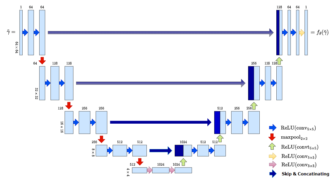
Figure 1: The U-net architecture for deep Calderón method. The input of the neural network is the reconstruction $\tilde{\gamma}$ by Calderón’s method with a resolution $64\times 64$ and the output is $f_{\theta}(\tilde{\gamma})$. Each box represents one layer of the neural network and numbers above the boxes are numbers of channels for each layer. The resolution is on the left bottom of the box. Each convolutional layer is equipped with an activation function ReLU($x$) = max(0,$x$). The blue blocks on the expanding part denote concatenation of blocks from the contracting part (i.e., skip connections).

The contracting part consists of several blocks, and each block includes convolution layer, activation layer and max-pooling layer. The max-pooling layers mainly help extract sharp features of the input images and reduce the size of the input image by computing the maximum over each nonoverlapping rectangular region. Specifically, the $i$th block in the contracting part can be expressed as

$$z^{\rm c}_{i+1}:=\tau_{i}^{\rm c}(z_{i}^{\rm c})=\mathcal{M}(\rho(W^{\rm c}_{i}\ast z_{i}^{\rm c}+b^{\rm c}_{i})),$$

where $\ast$ denotes the convolution operation, $W^{\rm c}_{i}$ and $b^{\rm c}_{i}$ refer to the convolution filter and bias vector, respectively, for the $i$th convolution layer, and $z_{i}^{\rm c}$ is the input image to the $i$th block (in the contracting part, and the input to the first block is the initial reconstruction $\tilde{\gamma}$ by Calderón’s method), $\mathcal{M}$ is the max-pooling layer, and $\rho:\mathbb{R}\to\mathbb{R}$ denotes a nonlinear activation function, applied componentwise to a vector. In this study, we employ the rectified linear unit (ReLU) activation function, i.e., $\rho(x)=\max(0,x)$ [31]. In practice, one may also include a batch / group normalization layer that aims to accelerate the training and reduce the sensitivity of the neural network initialization. Similarly, the expanding part also contains several blocks, each including a transposed convolution to extrapolate the input to an image of a larger size. One typical example of the $i$th block is given by

$$z^{\rm e}_{i+1}:=\tau^{\rm e}_{i}(z_{i}^{\rm e})=\mathcal{C}(\rho(\mathcal{T}(z_{i}^{\rm e},W^{\rm e}_{i},b^{\rm e}_{i}))),$$

where $\mathcal{T}$ denotes the transposed convolution operator, $W^{\rm e}_{i}$ and $b^{\rm e}_{i}$ refer to the corresponding convolutional filter and bias vector at the $i$th layer, and $\mathcal{C}$ is the concatenation layer. We use $\theta$ to denote the set of all unknown parameters including the convolutional and transposed convolutional filters and bias vectors, i.e., $\{W_{i}^{\rm c},b_{i}^{\rm c},W_{i}^{\rm e},b_{i}^{\rm e}\}$, that have to be learned from the training data via a suitable training procedure. In addition, we employ a skip connection from the input of the U-net to its output layer at each level, i.e.,

$$z_{i+1}^{\rm e}:=\tilde{\tau}_{i}^{\rm e}(z_{i}^{\rm e})=\tau_{L-i+1}^{\rm c}(z_{L-i+1}^{\rm c})+\tau_{i}^{\rm e}(z_{i}^{\rm e}),$$

where the integer $L$ is the total number of levels in the contracting part of the U-net. This architectural choice is useful since the input and output images are expected to share similar features, as is in most denoising type tasks. It enforces learning only the difference between the input and output which avoids learning the (abundantly known) part already contained in the input. Further, it is known to mitigate the notorious vanishing / exploding gradient problem during the training [22]. Then with $L$ contracting blocks and $L$ expanding blocks, the full CNN model $f_{\theta}$ can be represented as

$$f_{\theta}(\tilde{\gamma})=\tilde{\tau}_{L}^{\rm e}\circ\cdots\circ\tilde{\tau}_{1}^{\rm e}\circ\tau_{L}^{\rm c}\circ\cdots\circ\tau_{1}^{\rm c}(\tilde{\gamma}).$$

To measure the predictive accuracy of the afore-described CNN model $f_{\theta}$, we employ the mean squared error (MSE) as the loss function

$$\mathcal{L}(\theta)=\frac{1}{N}\sum_{n=1}^{N}\|f_{\theta}(\tilde{\gamma}_{n})-\gamma_{n}^{{\dagger}}\|_{F}^{2},$$

where $\gamma_{n}^{{\dagger}}$ denotes the true impedance corresponding to the $n$th inclusion sample (of the training dataset, which contains $N$ samples), $\tilde{\gamma}_{n}$ denotes the input image also corresponding to the $n$th inclusion sample, obtained by Calderón’s method, and $\|\cdot\|_{F}$ denotes the Frobenius norm of matrices. The loss $\mathcal{L}(\theta)$ is then minimized by a suitable optimizer, e.g., stochastic gradient descent [41], or Adam [29] or limited memory BFGS (all of which are directly available in many public software platforms, e.g., PyTorch or TensorFlow), in order to find an (approximate) optimal parameter $\theta^{*}$. The gradient of the loss $\mathcal{L}(\theta)$ with respect to the U-net parameter $\theta$ can be computed by automatic differentiation. In this work, the training is carried out in Google Colab engine with the Python library TensorFlow and the optimization is performed with Adam algorithm with a learning rate $10^{-4}$. The number of trainable parameters is 56,066,369 when the input image is of size $64\times 64$. The full implementation of the proposed method as well as the data used in the experiments will be made publicly available at the github link https://github.com/KwancheolShin/Deep-Calderon-method.git.

Conceptually, the proposed deep Calderón method can be viewed as a way of incorporating spatial / anatomical priori information into the EIT imaging algorithms [14, 19, 49]. This idea has been explored recently for Calderón’s method in [44, 45]. In the works [44, 45], the approximate location of each organ and their approximate constant conductivity are assumed to be known, since such information can be attained from other imaging modalities, e.g., CT-scans or ultrasound imaging, and then the prior information is incorporated to the scattering transformation which allows reconstructions with higher-resolution. Note that the method proposed in this work can be viewed as a new way of utilizing the spatial priori information to Calderón’s method.

3.2 Constructing training data

The success of the proposed deep Calderón’s method relies heavily on the availability of paired training data, as most supervised approaches do. In practice, it is often challenging or expensive to acquire many paired training data experimentally. Hence, we resort to simulated data. The training of a neural network is done on the simulated data as illustrated in Fig. 2. We use Case A in Fig. 3 for the illustration of our method but it is generally all the same for other examples. In order to generate the training data, from a picture of the tank, we extract the boundary data as in Fig. 2(b). Based on the boundary data, we construct the conductivity distribution $\gamma$ in Fig. 2(c). The mesh is on the square $[-1,1]^{2}$.

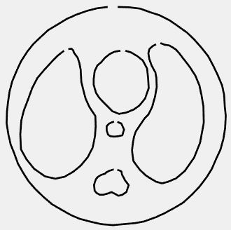
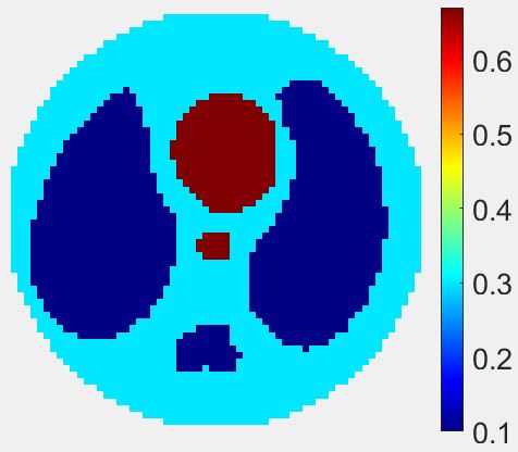
(a)	(b)	(c)

Figure 2: The construction of a realistic conductivity distribution from tank experiment. (a) The photo of the experimental tank, (b) the boundary of each organ, and (c) the conductivity distribution of the tank from which the EIT data is simulated by FEM solver.

Based on this single reference distribution, we simulate conductivity distributions by varying the shape and conductivity value. The detailed method will be described in the experimental study below. We denote these simulated conductivity distributions as $\{\gamma^{\dagger}_{n}\}_{n=1}^{N}$, where $N$ is the total number of conductivity distributions. Four instances of the simulated conductivity distributions $\{\gamma^{\dagger}_{n}\}_{n=1}^{N}$ for Case A are found in Fig. 4.

With the collection of the simulated conductivity distributions $\{\gamma_{n}^{\dagger}\}_{n=1}^{N}$, we solve the conductivity equation (1) with the applied current patterns (4) by the FEM [18] to get the simulated current-density/voltage data. Then, we reconstruct an estimate of the conductivity distribution with Calderón’s method, as explained in Section 2.2, on the square $[-1,1]^{2}$. It is well known that EIT is severely ill-posed, and small variations of the conductivity value in the interior of the domain $\Omega$ only lead to very tiny changes in the voltage measurement [9, 26]. In the experiment below, we are interested in very small inhomogeneities located far away from the domain boundary $\partial\Omega$, which can be resolved accurately only if the measurement data is highly accurate, and thus we investigate the addition of $0.01\%$ random noise to all voltage data below. Accordingly, we set the truncation radius $R$ to $1.3$. We denote the reconstructed images via Calderón’s method by $\{\tilde{\gamma}_{n}\}_{n=1}^{N}$. In this way, we obtain the paired training data $\{(\tilde{\gamma}_{n},\gamma^{\dagger}_{n})\}_{n=1}^{N}$. We randomly split $\{(\tilde{\gamma}_{n},\gamma^{\dagger}_{n})\}_{n=1}^{N}$ into two categories. $90\%$ of the them, denoted by $\{(\tilde{\gamma}_{j},\gamma^{\dagger}_{j})\}_{j=1}^{N_{1}}$, where $N_{1}$ is the number of the training data set, are used for the training of the neural network, and the remaining $N_{2}=N-N_{1}$ data are used for the validation of the neural network.

4 Experimental evaluation and discussions

The method is tested with four examples; see Fig. 3 for the schematic illustration of the phantoms. These setting are commonly use to evaluate EIT in a medical setting. Case A is a tank experiment with chest phantom filled with a saline bath, and each inclusion is made of agar based targets with added graphite to simulate the organs in a thorax; two lungs, a heart, a spine and an aorta. In Case B, the targets are made of agar with added salt and we put a copper pipe in one lung, simulating a high conductive pathology such as a tumor. In Case C, we put a PVC pipe in the same spot as in Case B to simulate a low conductive pathology such as an air trapping. In Case D, we have three slices of cucumber to demonstrate the reconstruction of complex-valued impedance. The method of simulating the training data and the network learning follow closely that in [21].

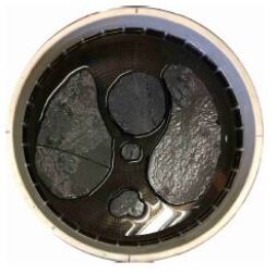
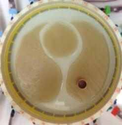
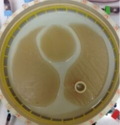
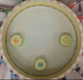
Case A	Case B	Case C	Case D

Figure 3: The illustration of four experimental settings. From the left to the right, Case A: a chest phantom with no pathology, Case B: a chest phantom with high conductive pathology in a lung, Case C: a chest phantom with low conductive pathology in a lung, and Case D: three slices of cucumber in a tank. Images are credited to [21, 44].

4.1 Case A: Case with no pathology

In this first case, we provide a preliminary validation of the proposed postprocessing strategy for Calderón’s method. To generate the simulated training data, we assign values for the conductivity to the regions of background (0.3), left lung (0.1), right lung (0.1), the heart (0.67), the aorta (0.67), and the spine (0.1). With this choice, we simulate $N=4096$ conductivity distributions $\{\gamma_{n}^{\dagger}\}_{n=1}^{N}$ by varying the size and the conductivity values of two lungs and the heart. Specifically, for the size, we give 10$\%$ random variation to the heart and 15$\%$ random variation to each lung as follows. We first compute the center of each organ by averaging each coordinate of the parameterized boundary points. From the center points, we compute the distance to each boundary points, and then multiply a uniformly distributed factor to the distance. The factors are random and independent for each organ. For the conductivity, we give 30$\%$ variation to each lung, 20$\%$ for the heart, and 10$\%$ for the background. The mesh size is $64\times 64$. The training takes only a few minutes with a batch size 256 and it is stopped after 12 epoches.

Fig. 4 shows the performance of Deep Calderón method on the validation set. Four instances are displayed to illustrate the results, where in each set of images, we show the simulated phantom $\gamma^{\dagger}$, the reconstruction $\tilde{\gamma}$ by Calderón’s method, and the output $f_{\theta}(\tilde{\gamma})$ from the neural network. Since Calderón’s method usually does not recover the full range of the conductivity distribution, the middle column images are under estimated in conductivity values. The four instances show (a) a phantom with big lungs and a high conductive heart, (b) a phantom with big lungs and a relatively low conductive heart, (c) a phantom with relatively small lungs and a high conductive heart, and (d) a phantom with relatively small lungs and a low conductive heart. We observe that the trained neural network is able to recover the size of the lungs well, and the shape of the heart is also well resolved and its size reasonably estimated. More precisely, the ratio of the number of heart cells in $f_{\theta}(\hat{\gamma})$ to that of the ground truth $\gamma^{\dagger}$ is about $0.95,1.10,0.93$ and $1.13$ for case (a), (b), (c) and (d), respectively, indicating that the hearts in (a) and (c) are under-estimated in size, whereas the hearts in (b) and (d) are over-estimated in size. Also, the network is able to recover the full range of conductivity values and also can estimate the approximate conductivity values for both lungs and the heart very well.

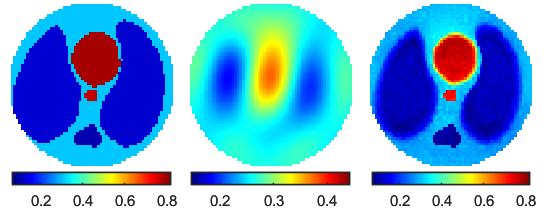
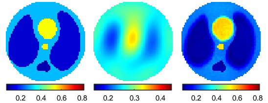
(a)	(b)
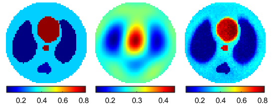
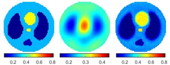
(c)	(d)

Figure 4: Exemplary reconstructions for Case A in four different situations. For each set of images, from left to right, they refer to simulated chest phantom $\gamma_{n}^{\dagger}$, reconstruction $\tilde{\gamma}$ by Calderón’s method, and the enhanced version $f_{\theta}(\tilde{\gamma})$.

4.2 Cases B and C: Case with a pathology in lungs

Next we illustrate the approach on the more challenging scenarios, where the lung contains one small inhomeneity, representing pathology or lesion, which is of much interest in practical imaging. Cases B and C are simulations with a pathology inside of one lung, cf. Fig. 5. To simulate the training data, we assign values for the conductivity to the region of background (0.19), left lung (0.123), right lung (0.123), the heart (0.323), the copper pipe (0.8), and the PVC pipe (0.01). We regard these distributions, depicted on the right column in Fig. 5, as the ground truth when we later evaluate the tank experimental data. We simulate $N=16384$ conductivity distributions by randomly varying the size and the conductivity of each organ. For the size, we give 10$\%$ variation to the heart and 25$\%$ to each lung, individually. The pathology inclusion is positioned randomly in one lung, and its size is fixed to be 2.2 cm in diameter throughout. In order to locate the inhomogeneity, we first compute the center $(x_{c},y_{c})$ of each lung by averaging $x$- and $y$-coordinates of the parameterized boundary points $(x_{b},y_{b})$, and then use a uniformly distributed random number $r$ between 0 to 1 to locate the center of the inhomogeneity $(x_{i},y_{i})$ as $(x_{i},y_{i})=(x_{c},y_{c})+r\times(x_{b}-x_{c},y_{b}-y_{c})$. In this way, the inhomogeneity may lie inside and on either of the two lungs and can overlap with the lung boundary. For the conductivity, we give 15$\%$ variation to the heart and 20$\%$ to each lung. One half of the data doesn’t include any pathology, 1/4 of the data include a high conductive pathology, and 1/4 of the data include a low conductive inclusion. The mesh size is $128\times 128$. The training takes about an hour with a batch size $128$ and it is stopped after 14 epoches.

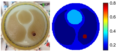
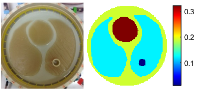
(a) Case B: phantom with a copper pipe	(b) Case C: phantom with a PVC pipe

Figure 5: Cases B and C: chest phantom with a pipe in one lung and their reference images.

We present the results on the validation dataset in Fig. 6, where the images in the second and third rows are for Cases B and C, respectively and the images in the top row do not contain small inclusions (pathology). These results show that the network is able to estimate the size and the conductivity of each organ surprisingly well. Also, the network is able to detect the abnormal inclusion in one lung. Fig. 7 shows the result with tank experimental data which were also used in [1, 44]. In each row, the difference images with Calderón’s method are shown in the middle column and the corresponding outputs from the network are shown in the last column. The data were collected using the ACE1 EIT system [35] on a circular tank with diameter 30 cm. The electrodes were 2.54 cm wide, and the level of saline bath was 1 cm. Adjacent current patterns were applied at the frequency 125 kHz with amplitude 3.3 mA. The copper pipe and PVC pipe are 1.6 cm and 2.2 cm in diameter. The results in Fig. 7 show that the network detects the boundary of each organ quite well. Also, the copper and PVC pipe is well detected. Visually, the output $f_{\theta}(\hat{\gamma})$ for Case B by the proposed deep Calderón’s method appears very fainted because the range of reconstruction is very broad due to the presence of the highly conductive copper pipe and this makes the difference in conductivity between the background and lung region relatively small. In Table 1, from the four reconstructions in Fig. 7, the conductivity values at four sample positions are displayed. In both cases B and C, the differences in conductivity between inclusions (H, L, P) and the background (B) are underestimated in $\tilde{\gamma}$ and are then amplified in $f_{\theta}(\tilde{\gamma})$. For Case B, $\tilde{\gamma}$, even though the conductivity at (P) is lower than that of (H), for $f_{\theta}(\tilde{\gamma})$ the value at (P) is higher than that of (H), which indicates that the amplification is nonlinear. Given that the amount of variation to the size and the conductivity of inclusions in the training data is quite large and the included pipes are very small in size for EIT imaging, the results are remarkable.

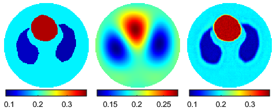
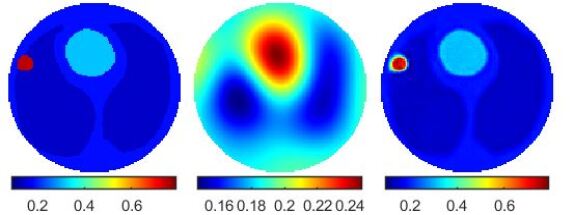
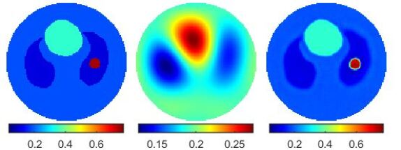
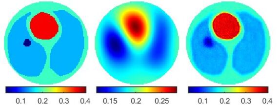
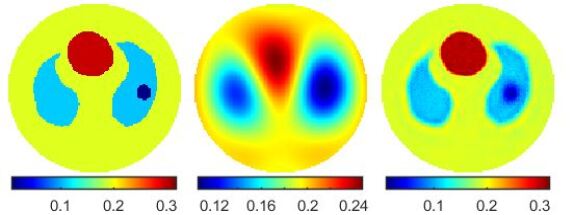
Figure 6: The reconstruction results with simulated data for Cases B (middle row) and C (bottom row). For each set of images, from left to right, they refer to simulated chest phantom $\gamma^{\dagger}$ (ground truth), the reconstruction $\tilde{\gamma}$ by Calderón’s method and enhanced version $f_{\theta}(\tilde{\gamma})$.

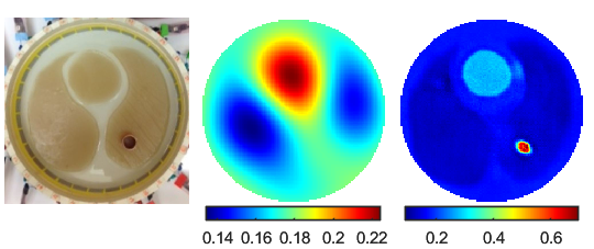
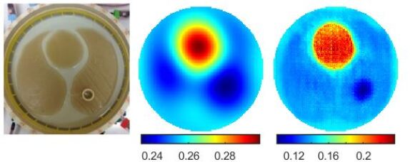
(a) Case B: copper pipe	(b) Case C: PVC pipe

Figure 7: The numerical results (from left to right, ground-truth, reconstruction $\tilde{\gamma}$ by Calderón’s method, the enhanced reconstruction $f_{\theta}(\tilde{\gamma})$) with experimental data for Cases B (left) and C (right).

			Case B		Case C
region	location	conductivity	$\tilde{\gamma}$	$f_{\theta}(\tilde{\gamma})$	$\tilde{\gamma}$	$f_{\theta}(\tilde{\gamma})$
Heart	(41,62)	.323	.224	.261	.199	.223
Background	(123,65)	.190	.169	.167	.157	.152
Lung	(71,30)	.123	.136	.127	.141	.130
Pipe	(89,89)	.8/.01	.174	.672	.134	.105

Table 1: Sample conductivity values for Cases B and C from the four reconstructions in Fig. 7. The first column represents the sampling regions: the heart (H), background (B), left lung (L), and the (copper/PVC) pipes (P). The second and third columns show the sampling positions (with respect to (row, column) number from the left-up corner while the size of the images is $124\times 124$) and the ground truth conductivity values.

4.3 Case D: Complex-valued targets

Case D simulates complex-valued targets with three slices of cucumber, see Fig. 8 for a schematic illustration of the tank. Each slice of cucumber is about 4.9 cm in diameter. Due to the cellular structure of cucumber, $\gamma(x)=\sigma(x)+i\omega\epsilon(x)$ is now complex-valued, and we reconstruct both the conductivity $\sigma(x)$ and the permittivity $\epsilon(x)$ simultaneously when the modulating frequency $\omega$ is known. The conductivity $\sigma(x)$ of the saline bath was 0.180 S/m. We assign values for the complex-valued admitivity to region of cucumbers (0.23 + 0.01$i$) and 0.18 to the region of background. In the simulation of the training data, three inclusions are randomly positioned (of equal size, 4.9 cm in diameter) without overlapping. In order to locate the three inclusions, we adopt the polar coordinate system, at the center of the tank, the circular domain $\Omega$ (centered at the origin and normalized to have radius 1). Now for the coordinates $(r,\theta)$ of the center of three inclusions, we randomly pick three radii $r$ each ranging in [0, 0.15], [0.3, 0.45] and [0.6, 0.75] in order to avoid the overlapping of the inclusions but also that they have a good coverage of the domain $\Omega$, and then choose the angle $\theta$ randomly distributed ranging in [0, $2\pi$]. We give 10$\%$ random variation to the conductivity of each inclusion, and does not change the size of the inclusions. The size of the training data set is $N=4096$ on a mesh $64\times 64$. Training with complex-valued imaging was studied in [33]. However, in this study, we train the neural network with only real part, and then use the single trained neural network for the validation of both real and imaginary parts. Also, we normalize the training data to the range $[0,1]$.

We test the proposed method with two examples: tank experimental data and a simulated data. The experimental data was collected using the ACE 1 system at a modulating frequency $\omega=125\text{ kHz}$, excited with adjacent current patterns with an amplitude 3.3 mA. The level of saline bath was 1.6 cm. In Fig. 9, we show the approximate ground truth that is extracted from a photo of the tank, reconstruction by Calderón’s method and the deep version, for the real and imaginary parts separately. Since the training data is normalized to the range $[0,1]$, when we feed the real part $\Re(\tilde{\gamma})$ (or imaginary part $\Im(\tilde{\gamma})$) to the trained neural network, we normalize it to $[0,1]$ as well. From Fig. 9, we can see that $f_{\theta}(\Re(\tilde{\gamma}))$ (or $f_{\theta}(\Im(\tilde{\gamma}))$ ranges from 0 to about 1.1 and the location of three inclusions are well detected for both real and imaginary parts. For the second test example, we have only one inclusion, cf. the second row of Fig. 9. Even though the case with one inclusion is not in the training dataset, the proposed method can still produce reasonable reconstructions, showing the high out-of-distribution robustness of the proposed approach. This property is highly desirable since in some practical applications, it might be difficult to exactly anticipate the number of inclusions a priori in the training data.

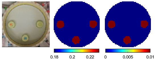
Figure 8: Case D. The images (from left to right) are the picture of the tank, real and imaginary parts of the approximate ground truth.

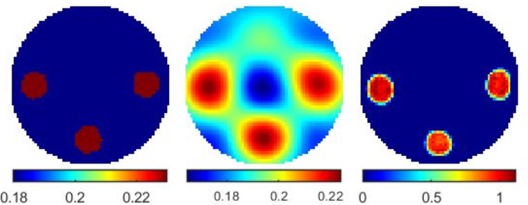
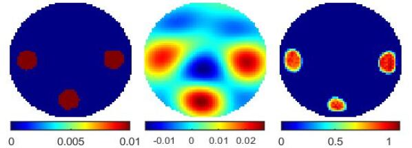
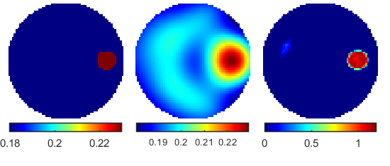
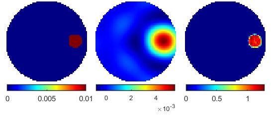
(a) real part	(b) imaginary part

Figure 9: Reconstructions for Case D with experimental tank data (top row), cf. Fig. 8 and with simulated data with a single inclusion (bottom row). The images from left to right are the approximated ground truth, Calderón reconstruction and the enhanced version.

4.4 Further discussions

In this work, we have proposed an enhanced Calderón method via post-processing using DNNs, called deep Calderón’s method, and demonstrated its superior performance over classical Calderón’s method on several medically important settings. Intuitively, this can be understood as follows. Denote the inversion by Calderón’s method by $\mathcal{I}^{\rm cm}:\Lambda_{\gamma}\to\tilde{\gamma}$, and the post-processing by U-net by $f_{\theta}:\tilde{\gamma}\rightarrow f_{\theta}(\tilde{\gamma})$. While the inverse map $\mathcal{I}:\Lambda_{\gamma}\to\gamma$ is nonlinear in nature, as Calderón’s method is a linearized and regularized method by the low-pass filtering, the inversion $\mathcal{I}^{\rm cm}$ loses the nonlinear nature of $\mathcal{I}$. Since DNNs are universal approximators [23], deep Calderón’s method $f_{\theta}\circ\mathcal{I}^{\rm cm}:\Lambda_{\gamma}\to\tilde{\gamma}$ might compensate the loss of non-linearity in $\mathcal{I}^{\rm cm}$ and therefore it can be a better approximation to $\mathcal{I}$ than the linearised inversion scheme $\mathcal{I}^{\rm cm}$. This effect has been numerically confirmed by the experiments in this work.

The neural network $f_{\theta}$ cannot be independent of the training data and therefore might be different for individual example. Since the structure of a human body is much more complicated than just lungs and the heart, in order to apply the proposed method to a more physically realistic setting including thorax imaging, one must generate a load of training data with arbitrary inclusions to learn the neural network. Moreover, the deep Calderón method also depends on many hyper parameters in the experimental setting and Calderón’s method, e.g., the truncation radius $R$, the injected current pattern and general measurement settings. Hence, constructing a universal neural network is hardly attainable and one will always require some prior knowledge about the target to train a neural network and therefore the suggest method would be case-specific. In this paper, an approximate location, a constant conductivity and the shape of each inclusion are assumed to be known as prior information. The deep Calderón method can be viewed as a way of incorporating such implicit prior information into the reconstruction algorithm.

In the reconstructions by Calderón’s method, we have chosen the truncation radius $R$ by a rule of thumb as there is no unified method for choosing $R$ as yet. Having a small $R$ results in a high degree of regularization featuring a stable but blurry reconstruction, and a bigger $R$ leads more detailed but less unstable reconstructed images. Therefore, one may employ a multi-channel network by training the neural network with a large collection of input images for different $R$ simultaneously. The application of deep Calderón method to human data involving a moving boundary modeling is also of much interest.

5 Conclusions

We have proposed a deep Calderón method and evaluated its performance on several important settings. It is observed that the proposed method can significantly improve the reconstructed images by Calderón’s method: size, shape and location of the inclusions are well detected, and the boundary of inclusions is sharpened to have resulted in images with much higher resolution. Moreover, the underestimated conductivity values are well adjusted. Also, even a very small abnormal inclusion can be singled out with the proposed method which is almost impossible with the original Calderón’s method (or other direct reconstrution methods). For complex-valued targets, a single trained neural network using the real part of the reconstructions can be used for the post-processing of both real and imaginary parts. These results indicate that the proposed enhancement strategy is indeed very effective and holds big potentials for certain applications, especially in the medical context.

References

- [1] M. Alsaker and J. L. Mueller. Use of an optimized spatial prior in D-bar reconstructions of EIT tank data. Inverse Probl. Imaging, 12(4):883–901, 2018.
- [2] H. Ammari and H. Kang. Reconstruction of Small Inhomogeneities from Boundary Measurements. Springer-Verlag, Berlin, 2004.
- [3] H. Ammari, H. Kwon, S. Lee, and J. K. Seo. Mathematical framework for abdominal electrical impedance tomography to assess fatness. SIAM J. Imaging Sci., 10(2):900–919, 2017.
- [4] H. Ammari, J. K. Seo, and T. Zhang. Mathematical framework for multi-frequency identification of thin insulating and small conductive inhomogeneities. Inverse Problems, 32(10):105001, 23, 2016.
- [5] M. C. Bachmann, C. Morais, G. Bugedo, A. Bruhn, A. Morales, J. B. Borges, E. Costa, and J. Retamal. Electrical impedance tomography in acute respiratory distress syndrome. Critical Care, 22:263, 2018.
- [6] R. Barbano, v. Kereta, A. Hauptmann, S. R. Arridge, and B. Jin. Unsupervised knowledge-transfer for learned image reconstruction. Inverse Problems, 38(10):104004, 28, 2022.
- [7] E. Beretta, S. Micheletti, S. Perotto, and M. Santacesaria. Reconstruction of a piecewise constant conductivity on a polygonal partition via shape optimization in EIT. J. Comput. Phys., 353:264–280, 2018.
- [8] J. Bikowski and J. L. Mueller. 2D EIT reconstructions using Calderón’s method. Inverse Probl. Imaging, 2(1):43–61, 2008.
- [9] L. Borcea. Electrical impedance tomography. Inverse Problems, 18(6):R99–R136, 2002.
- [10] A.-P. Calderón. On an inverse boundary value problem. In Seminar on Numerical Analysis and its Applications to Continuum Physics (Rio de Janeiro, 1980), pages 65–73. Soc. Brasil. Mat., Rio de Janeiro, 1980.
- [11] M. Cheney, D. Isaacson, J. C. Newell, S. Simske, and J. Goble. NOSER: An algorithm for solving the inverse conductivity problem. Int. J. Imag. Syst. Technol., 2(2):66–75, 1990.
- [12] Y. T. Chow, K. Ito, and J. Zou. A direct sampling method for electrical impedance tomography. Inverse Problems, 30(9):095003, 25, 2014.
- [13] D. C. Dobson and F. Santosa. An image-enhancement technique for electrical impedance tomography. Inverse Problems, 10(2):317–334, 1994.
- [14] B. M. Eyüboglu, T. C. Pilkington, and P. D. Wolf. Estimation of tissue resistivities from multiple-electrode impedance measurements. Phys. Med., Biol., 39(1):1–17, 1994.
- [15] Y. Fan and L. Ying. Solving electrical impedance tomography with deep learning. J. Comput. Phys., 404:109119, 19, 2020.
- [16] G. Franchineau, N. Bréchot, G. Lebreton, G. Hekimian, A. Nieszkowska, J.-L. Trouillet, P. Leprince, J. Chastre, C.-E. Luyt, A. Combes, and M. Schmidt. Bedside contribution of electrical impedance tomography to setting positive end-expiratory pressure for extracorporeal membrane oxygenation-treated patients with severe acute respiatory distress syndrome. Am. J. Respir. Crit. Care Med., 196(4):447–457, 2017.
- [17] M. Gehre and B. Jin. Expectation propagation for nonlinear inverse problems – with an application to electrical impedance tomography. J. Comput. Phys., 259:513–535, 2014.
- [18] M. Gehre, B. Jin, and X. Lu. An analysis of finite element approximation in electrical impedance tomography. Inverse Problems, 30(4):045013, 24, 2014.
- [19] M. Glidewell and K. T. Ng. Anatomically constrained electrical impedance tomography for anisotropic bodies via a two-step approach. IEEE Trans. Med. Imag., 14(3):498–503, 1995.
- [20] R. Guo and J. Jiang. Construct deep neural networks based on direct sampling methods for solving electrical impedance tomography. SIAM J. Sci. Comput., 43(3):B678–B711, 2021.
- [21] S. J. Hamilton and A. Hauptmann. Deep D-bar: Real-time electrical impedance tomography imaging with deep neural networks. IEEE Trans. Med. Imag., 37(10):2367–2377, 2018.
- [22] K. He, X. Zhang, S. Ren, and J. Sun. Deep residual learning for image recognition. In Proceedings of the IEEE Conference on Computer Vision and Pattern Recognition (CVPR), pages 770–778, 2016.
- [23] K. Hornik, M. Stinchcombe, and H. White. Multilayer feedforward networks are universal approximators. Neural Networks, 2(5):359–366, 1989.
- [24] C. M. Hyun, H. P. Kim, S. M. Lee, S. Lee, and J. K. Seo. Deep learning for undersampled MRI reconstruction. Phys. Med. Biol., 63(13):135007, 2018.
- [25] D. Isaacson, J. L. Mueller, J. C. Newell, and S. Siltanen. Reconstructions of chest phantoms by the d-bar method for electrical impedance tomography. IEEE Trans. Med. Imag., 23(7):821–828, 2004.
- [26] B. Jin, T. Khan, and P. Maass. A reconstruction algorithm for electrical impedance tomography based on sparsity regularization. Internat. J. Numer. Methods Engrg., 89(3):337–353, 2012.
- [27] K. H. Jin, M. T. McCann, E. Froustey, and M. Unser. Deep convolutional neural network for inverse problems in imaging. IEEE Trans. Image Proc., 26(9):4509–4522, 2017.
- [28] E. Kang, J. Min, and J. C. Ye. A deep convolutional neural network using directional wavelets for low-dose X-ray CT reconstruction. Med. Phys., 44(10):e360–e375, 2017.
- [29] D. P. Kingma and J. Ba. Adam: A method for stochastic optimization. In 3rd International Conference for Learning Representations, San Diego, 2015.
- [30] A. Kirsch and N. Grinberg. The Factorization Method for Inverse Problems. Oxford University Press, Oxford, 2008.
- [31] Y. LeCun, L. Bottou, G. B. Orr, and K.-R. Müller. Efficient BackProp. In G. Montavon, G. Orr, and K. Müller, editors, Neural Networks: Tricks of the Trade, pages 9–48. Springer, Heidelberg, 1998.
- [32] X. Li, Y. Zhou, J. Wang, Q. Wang, Y. Lu, X. Duan, Y. Sun, J. Zhang, and Z. Liu. A novel deep neural network method for electrical impedance tomography. Trans. Instit. Measur. Control, 41(14):4035–4049, 2019.
- [33] A. Liu, L. Yu, Z. Zeng, X. Xie, Y. Guo, and Q. Shao. Complex-valued U-net for PolSAR image semantic segmentation. J. Phys.: Conf. Ser., 2010:012102, 2021.
- [34] S. Martin and C. T. M. Choi. A post-processing method for three-dimensional electrical impedance tomography. Sci. Rep., page 7212, 2017.
- [35] M. M. Mellenthin, J. L. Mueller, E. D. L. B. de Camargo, F. S. de Moura, T. B. R. Santos, R. G. Lima, S. J. Hamilton, P. A. Muller, and M. Alsaker. The ACE1 electrical impedance tomography system for thoracic imaging. IEEE Trans. Instrum. Measure., 68(9):3137–3150, 2019.
- [36] J. L. Mueller and S. Siltanen. The D-bar method for electrical impedance tomography—demystified. Inverse Problems, 36(9):093001, 28, 2020.
- [37] P. A. Muller and J. L. Mueller. Reconstruction of complex conductivities by Calderón’s method on subject-specific domains. In 2018 International Applied Computational Electromagnetics Society Symposium (ACES), 2018.
- [38] P. A. Muller, J. L. Mueller, and M. M. Mellenthin. Real-time implementation of Calderón’s method on subject-specific domains. IEEE Trans. Med. Imag., 36(9):1868–1875, 2017.
- [39] R. Murthy, Y.-H. Lin, K. Shin, and J. L. Mueller. A direct reconstruction algorithm for the anisotropic inverse conductivity problem based on Calderón’s method in the plane. Inverse Problems, 36(12):125008, 21, 2020.
- [40] C. Putensen, B. Hentze, S. Muenster, and T. Mudeers. Electrical impedance tomography for cardio-pulmonary monitoring. J. Clin. Med., 8(8):1176, 2019.
- [41] H. Robbins and S. Monro. A stochastic approximation method. Ann. Math. Statistics, 22:400–407, 1951.
- [42] O. Ronneberger, P. Fischer, and T. Brox. U-net: Convolutional networks for biomedical image segmentation. In N. Navab, J. Hornegger, W. M. Wells, and A. F. Frangi, editors, Medical Image Computing and Computer-Assisted Intervention – MICCAI 2015, pages 234–241, Cham, 2015. Springer International Publishing.
- [43] K. Shin, S. U. Ahmad, and J. L. Mueller. A three dimensional Calderón-based method for eit on the cylinderical geometry. IEEE Trans. Biomed. Eng., 68(5):1487–1495, 2021.
- [44] K. Shin and J. L. Mueller. A second order Calderón’s method with a correction term and a priori information. Inverse Problems, 36(12):124005, 22, 2020.
- [45] K. Shin and L. Mueller, Jennifer. Calderón’s method with a spatial prior for 2-D EIT imaging of ventilation and perfusion. Sensors, 21(6):5636, 2021.
- [46] S. Siltanen, J. Mueller, and D. Isaacson. An implementation of the reconstruction algorithm of A. Nachman for the 2D inverse conductivity problem. Inverse Problems, 16(3):681–699, 2000.
- [47] C. Tan, S. Lv, F. Dong, and M. Takei. Image reconstruction based on convolutional neural network for electrical resistance tomography. IEEE Sensors J., 19(1):196–204, 2019.
- [48] V. Tomicic and R. Cornejo. Lung monitoring with electrical impedance tomography: technical considerations and clinical applications. J. Thor. Dis., 11(7):3122–3135, 2019.
- [49] M. Vauhkonen, J. P. Kaipio, E. Somersalo, and P. A. Karjalainen. Electrical impedance tomography with basis constraints. Inverse Problems, 13(2):523–530, 1997.
- [50] B. Vogt, Z. Zhao, P. Zabel, N. Weiler, and I. Frerichs. Regional lung response to bronchodilator reversibility testing determined by electrical impedance tomography in chronic obstructive pulmonary disease. Am. J. Physiol. Lung. Cell Mol. Physiol., 311(1):L8–L19, 2016.
- [51] Z. Wei, D. Liu, and X. Chen. Dominant-current deep learning scheme for electrical impedance tomography. IEEE Trans. Biomed. Eng., 66(9):2546–2555, 2019.
- [52] E. J. Woo, P. Hua, J. G. Webster, and W. J. Tompkins. Finite-element method in electrical impedance tomography. Med. Biol. Eng. Comput., 32:530–536, 1994.
- [53] Y. Wu, B. Chen, K. Liu, C. Zhu, H. Pan, J. Jia, H. Wu, and J. Yao. Shape reconstruction with multiphase conductivity for electrical impedance tomography using improved convolutional neural network method. IEEE Sensors J., 21(7):9277–9287, 2021.